HAL Id: hal-01164751https://hal.archives-ouvertes.fr/hal-01164751

Submitted on 17 Jun 2015

HAL is a multi-disciplinary open accessarchive for the deposit and dissemination of sci-entific research documents, whether they are pub-lished or not. The documents may come fromteaching and research institutions in France orabroad, or from public or private research centers.

L’archive ouverte pluridisciplinaire HAL, estdestinée au dépôt et à la diffusion de documentsscientifiques de niveau recherche, publiés ou non,émanant des établissements d’enseignement et derecherche français ou étrangers, des laboratoirespublics ou privés.

Boolean Network Identification from Multiplex TimeSeries Data

Max Ostrowski, Loïc Paulevé, Torsten Schaub, Anne Siegel, CaritoGuziolowski

To cite this version:Max Ostrowski, Loïc Paulevé, Torsten Schaub, Anne Siegel, Carito Guziolowski. Boolean NetworkIdentification from Multiplex Time Series Data. CMSB 2015 - 13th conference on ComputationalMethods for Systems Biology, Sep 2015, Nantes, France. pp.170-181, �10.1007/978-3-319-23401-4_15�.�hal-01164751�

Boolean Network Identification from MultiplexTime Series Data

M. Ostrowski1?, L. Pauleve2?, T. Schaub1, A. Siegel3,, C. Guziolowski4

1 Potsdam University, Computer Science Department, Postdam, Germany.2 CNRS, Universite Paris-Sud LRI-UMR 8623, Orsay, France

3 CNRS, Universite de Rennes 1, IRISA-UMR 6074, Rennes, France4 Ecole Centrale de Nantes, IRCCyN UMR CNRS 6597, Nantes, France.

Abstract. Boolean networks (and more general logic models) are use-ful frameworks to study signal transduction across multiple pathways.Logical models can be learned from a prior knowledge network structureand multiplex phosphoproteomics data. However, most efficient and scal-able training methods focus on the comparison of two time-points andassume that the system has reached an early steady state. In this paper,we generalize such a learning procedure to take into account the timeseries traces of phosphoproteomics data in order to discriminate Booleannetworks according to their transient dynamics. To that goal, we exhibita necessary condition that must be satisfied by a Boolean network dy-namics to be consistent with a discretized time series trace. Based onthis condition, we use a declarative programming approach (Answer SetProgramming) to compute an over-approximation of the set of Booleannetworks which fit best with experimental data. Combined with model-checking approaches, we end up with a global learning algorithm andcompare it to learning approaches based on static data.

1 Introduction

Generic prior knowledge about canonical cell signaling networks can be retrievedfrom database sources. They provide a first insight on how cells respond totheir environment by triggering processes such as growth, survival, apoptosis(cell death), and migration. However, little is known about the exact chainingand composition of signaling events within these networks in specific cells andspecific conditions, as provided by the simulations of predictive mathematicalmodels (e.g. a set of differential equations or a set of logic rules). When buildingpredictive models, the parameters of a model (built accordingly to generic priorknowledge) can be fitted to the data to obtain the most plausible model fora specific cell type, if enough experimental data is available. This is normallyachieved by defining an objective fitness function to be optimized. In this context,post-translational modifications, notably protein phosphorylation, play a keyrole in signaling. They are very useful for the training of model parameters

? Co-first authors

through the use of multiplex phosphorylation assays, a recent form of high-throughput data providing information about protein-activity modifications ina specific cell type upon various perturbations (clamping) [1].

Boolean logical networks [12] provide a simple yet powerful qualitative frame-work which has become very popular during the last decade to model signalingor regulatory networks [16]. In contrast to quantitative methods which permitfine-grained kinetic analysis, qualitative approaches allow for addressing large-scale biological networks. In this context, the manual identification of logic rulesunderlying the system has been addressed under different hypotheses and meth-ods [4]. Although, scalable methods restrain themselves to learning models fromtwo time points (start; end), assuming the system has reached an early steady-state when the measurements are performed. As shown in [14], this assumptionprevents capturing important characteristics of signaling networks such as loops.

The goal of this paper is to introduce a new method to infer Boolean net-works (BNs) from time series datasets which scales to the size of currently studiedBNs. Given multiplex time series data from the measurement of a partial set ofbiological entities under different experimental conditions, we want to identifyall the BNs that have a structure compatible with a given prior knowledge in-teraction graph and that can reproduce all the (experimentally) observed timeseries. Time series data are assumed incomplete, i.e., only a subset of networkcomponents are observed, with measurements made at discrete time points andwith normalized continuous values. It is possible that no BN, constrained by theprior interaction graph, reproduces all the input time series. In such a case weintroduce a fitness function to measure the distance between a trace of a BNsimulation and a measured time series. Therefore, we aim to infer the BNs whosedynamics contains traces with the best fitness to all measurements.

Our approach relies on the combination of several techniques. First, we intro-duce a necessary condition for a discretized time series data to be the trace of aBN. This provides an over-approximation of the successive reachability proper-ties, leading to reject BNs that cannot reproduce the time series without a costlyexhaustive analysis of the dynamics. Then, we use efficient declarative program-ming approaches (Answer Set Programming; ASP) to enumerate BNs whichapproximate the best experimental data while satisfying the necessary conditionon the dynamics. At the end, we obtain a set of BNs associated with traces whichboth satisfy the necessary condition and optimally fit with experimental data.Because of the reachability over-approximation, part of the returned BNs cannotreproduce the associated Boolean traces. Such false positives can be detected aposteriori using a model-checking approach on the returned results.

We evaluated our inference method on synthetic data generated from BNsbetween 13 and 17 nodes. On those BNs, six nodes have been selected as observ-able, and several experimental conditions have been simulated. Our prototypeimplementation has been able to identify efficiently all BNs satisfying the neces-sary condition with a very low rate of false positives. Finally, we estimated theadded-value of models identified with our method on the full time series withmodels learned from two time points, considered as a steady state.

2 Boolean Network Identification

2.1 Admissible Boolean Networks and multiplex time series data

Boolean Networks (BNs). A BN with n components {1, . . . , n} consists of a tuple

of n functions F = (f1, . . . , fn) where each function fi : Bn → B, B ∆= {0, 1},

i ∈ {1, . . . , n}, associates to each global state x ∈ Bn of the network with the nextvalue of the i-th component. The value of the i-th component in x is noted xi.The transitions between global states of the network are specified with a reflexivetransition relation → ⊆ Bn×Bn. The transitive closure of → is denoted by →∗.Given x, x′ ∈ Bn, x→∗ x′ if and only if, either x = x′, or x→ · · · → x′.

Concrete semantics for the transition relation. Several definitions of the tran-sition relation → can be used depending on the update schedule of the compo-nents [2], ranging from so-called parallel (or synchronous) updates where eachtransition updates the value of all the components, to the asynchronous updatewhere each transition updates the value of only one component chosen non-deterministically. As the over-approximation results presented in this article areindependent from the update schedule, we use the general definition, where anynumber of components can be updated during a transition: for any x, x′ ∈ Bn,

x→ x′∆⇔ ∀i ∈ {1, . . . , n}, x′i 6= xi ⇒ x′i = fi(x) . (1)

Prior Knowledge Network and admissible BNs. An interaction graph betweenn components is a digraph between nodes {1, . . . , n} where each edge is signed,i.e., either positive or negative. The interaction graph of a BN F , noted IG(F ),has a positive (resp. negative) edge from node j to node i if and only if thereexists x, x′ ∈ Bn which are identical except on the j-th coordinate where xj = 0and x′j = 1 and such that fi(x) < fi(x

′) (resp. fi(x) > fi(x′)).

In the rest of the paper, the Prior Knowledge Network (PKN) is an interac-tion graph which delimits the set of admissible BNs: a BN F is admissible withrespect to a PKN G if and only if IG(F ) is a sub-graph of G and IG(F ) has atone most (signed) edge between two nodes.

Multiplex Time Series Data. We consider classical biology experimental set-tings where the activity of a subset of biological species is observed over time,at discrete time points, in different experimental conditions, ranging over var-ious input signals and clamping operations. Clampings consist of a subset Aof components with a forced activation, and a subset I of components with aforced inhibition. Given a BN F = (f1, . . . , fn), the corresponding clamped BNF[A,I] = (f ′1, . . . , f

′n) is defined for all i ∈ {1, . . . , n} as:

f ′i∆=

x 7→ 1 if i ∈ Ax 7→ 0 if i ∈ Ifi otherwise.

Without loss of generality, we assume that the time series data relate to theobservation of m ≤ n nodes that match the nodes {1, . . . ,m} of the BN (so thenodes {m+ 1, . . . , n} are not observed). The observations consist of normalizedcontinuous values: a time series of k data points is denoted by T = (t1, . . . , tk),with ∀j ∈ {1, . . . , k}, tj ∈ [0; 1]m.

Hereafter, we consider a simple binarization of observations using a 0.5threshold: given a continuous observation tji ∈ [0; 1] of a component, its Boolean

value is noted η(tji ) where η(tji )∆= 1 when tji ≥ 0.5, and η(tji )

∆= 0 otherwise. The

distance between a binary sequence X = (x1, . . . , xk), where ∀i ∈ {1, . . . , k}, xi ∈Bm, and a time series T is evaluated with the standard Mean Squared Error :

mse(X,T )∆=

√∑kj=1

∑mi=1 (xji − t

ji )

2.

2.2 Over-approximation of Boolean network verification

Given a BN F and a pair of states x, y ∈ Bn, checking the reachability of yfrom x (x →∗ y) is a standard model-checking task, known to have a limitedscalability due to its theoretical complexity (NP-complete [11]). In this section,we introduce a so-called meta-state semantics (⇒) for BNs. From such seman-tics, we express a necessary condition for reachability in the concrete semantics(→), referred to as support consistency ( ∗). Meta-state semantics offers prop-erties (notably monotonicity) that make support consistency efficient to verify,in particular with ASP. However, support consistency is not a sufficient condi-tion for reachability, so this approach may lead to false positives but guaranteesthe absence of false negatives. Therefore, we will apply exact model-checkingapproaches on the inferred BNs in order to rule out false positives. Thanks tothe over-approximation criteria, one can expect that the set of BNs satisfyingthe necessary condition is small compared to the full domain of BNs delimitedby the PKN, leading to a global gain in terms of performance.

Meta-state semantics. A meta-state u of dimension n is a vector of n non-empty

subsets of B, noted M ∆= {{0}, {1}, {0, 1}}; the set of meta-states is Mn. In the

following, meta-states characterize a set of Boolean states: a state x ∈ Bn belongsto a meta-state u ∈Mn, noted x ∈ u, iff each Boolean component xi belongs tothe set ui, i.e., ∀i ∈ {1, . . . , n}, xi ∈ ui. Given a state x ∈ Bn, x is the meta-statesuch that ∀i ∈ {1, . . . , n}, xi = {xi}. In the scope of a BN F = (f1, . . . , fn),we define a reflexive transition relation between meta-states ⇒ ⊆ Mn ×Mn asfollows: from a meta-state u, there is one transition for each i ∈ {1, . . . , n} whichadds to ui all the possible values of the function fi applied to every x ∈ u:

u⇒ v∆⇔ ∃i ∈ {1, . . . , n}, v = 〈u1, . . . , ui ∪ {fi(x) | x ∈ u}, . . . un〉 . (2)

Several properties arise from this definition, in particular u ⇒ v implies that∀i ∈ {1, . . . , n}, ui ⊆ vi; therefore x ∈ u ⇒ x ∈ v (monotonicity). Moreover,ui 6= vi if and only if vi = {0, 1} and ∃x ∈ u such that fi(x) /∈ ui.

Lemma 1 establishes the consistency of the meta-semantics (⇒) with the con-crete semantics (→): given x, y ∈ Bn, x → y requires that there exists a meta-state u such that y ∈ u and x ⇒∗ u, where ⇒∗ is the transitive closure of ⇒.

Lemma 1. ∀x, y ∈ Bn, x→ y =⇒ ∃u ∈Mn, y ∈ u : x⇒∗ u.

Proof. Assuming x → y, let us define the set I∆= {i ∈ {1, . . . , n} | yi 6= xi}.

From equation (1), ∀i ∈ I, yi = fi(x). Let us assume that for some strict subsetJ ( I, ∃v ∈ Mn, x⇒∗ v with ∀i ∈ J , yi ∈ vi. It is notably the case with J = ∅.By induction, we show that, for any k ∈ I \ J , ∃u ∈ Mn such that x⇒∗ v ⇒ uwith ∀i ∈ J ∪ {k}, yi ∈ ui. Remarking that x ∈ v and defining u ∈ Mn such asui = vk ∪ {fk(z) | z ∈ v} if i = k and ui = vi if i 6= k, we obtain that v ⇒ u,with yk = fk(x) ∈ uk. ut

Such a necessary condition for reachability can be furthermore refined byensuring that for each component i ∈ {1, . . . , n} that is equal in x and y, if allmeta-states u containing y with x⇒∗ u are such that ui = {0, 1}, then u containsa state z with fi(z) = yi = xi. Intuitively, this refinement ensures that if thei-th component has to temporarily change its value for reaching y, a state fromwhich it can recover its initial (and final) value has to be reached in between.Such a condition is referred to as support consistency (definition 1). Theorem 1states that support consistency is a necessary condition for reachability.

Definition 1 (Support Consistency ( ∗)). A state x ∈ Bn is support-consistent with y ∈ Bn, denoted by x ∗ y, if and only if there exists u ∈ Mn

with x ⇒∗ u such that y ∈ u and for all i ∈ {1, . . . , n} where yi = xi, ui ={0, 1} =⇒ ∃z ∈ u : fi(z) = yi.

Theorem 1. ∀x, y ∈ Bn, x→∗ y =⇒ x ∗ y.

Proof. Let us consider any tuple of states (x1, . . . , xk) with x1 = x, xk = y, and∀j ∈ {1, . . . , k − 1}, xj → xj+1. From lemma 1, ∃u ∈ Mn such that x⇒∗ u and∀j ∈ {1, . . . , k}, xk ∈ u. If for all such u, for any i ∈ {1, . . . , n}, ui = {0, 1}implies that there exists l ∈ {1, . . . , k} with xli 6= xi. If yi = xi, there necessarilyexists m ∈ {l, . . . , k − 1} such that fi(x

m) = yi. Therefore xm ∈ u. ut

2.3 Optimization with respect to time series data

Our objective is to infer BNs that are admissible with a given PKN and thatverify the sequential reachability of binary states in Bm that are as close aspossible to a given time series data and its associated experimental settings.

Distance between a time series data and a BN. Given a time series T withassociated clamping A, I, the distance between a BN F and (T,A, I), notedmse(F[A,I], T ), is the minimal MSE between T and a sequence of binary states

X = (x1, . . . , xk), with ∀j ∈ {1, . . . , k}, xj ∈ Bn, that are successively reachable

in F[A,I]: x1 →∗ x2 . . . →∗ xk. We notice that the lowest possible mse(X,T )

among all Boolean traces is the MSE between T and its binarization η(T ) =

((η(t1i ))i=1...m, · · · , (η(tki ))i=1...m). Let us call MSET∆= mse(η(T ), T ) this min-

imum MSE which is intrinsic to the time series T and to the threshold forbinarization (0.5); mse(F[A,I], T ) ≥ MSET . Whenever mse(F[A,I], T ) = MSET ,we say the BN F reproduces the time series data T .

Relaxing the semantics constraint. In order to prevent an exhaustive explorationof the BN dynamics for characterizing the sequences of reachable (→∗) Booleanstates, we consider any sequence X = (x1, . . . , xk), with ∀j ∈ {1, . . . , k}, xj ∈ Bn,that are support-consistent ( ∗), i.e., x1 ∗ x2 . . . ∗ xk in the scope of theBN F[A,I]. The MSE of such a support-consistent Boolean state sequence Xw.r.t. the time series T is noted mse(X,T ); and the minimal distance amongall support-consistent sequences in F[A,I] with T is referred to as mse(F[A,I], T ).Because any reachable sequence is support-consistent (theorem 1), we obtainthat mse(F[A,I], T ) ≥ mse(F[A,I], T ) ≥ MSET ; and in particular mse(F[A,I], T ) 6=mse(F[A,I], T ) only if none of the support-consistent sequences X with minimalmse(X,T ) are actually sequences of reachable Boolean states. In such cases, Fis a false positive. Determining if F is a true positive can be done a posterioriwith a model-checking approach: if mse(F[A,I], T ) = MSET , we check that η(T )is a valid sequence of reachable states in F[A,I]; otherwise, we check the validitywith respect to reachability of at least one sequence X with minimal mse(X,T ).

Optimization problem. We consider a PKN G and a set of r multiplex timeseries D = (T 1, A1, I1), . . . , (T r, Ar, Ir). The distance between a BN F and

the dataset is the sum of distances mse(F,D)∆=

∑rl=1 mse(F[Al,Il], T

l). Theoptimization procedure identifies the BNs compatible with the PKN G that havethe minimal distance mse(F,D). In the scope of this paper, we enforce that eachnon-observed node starts with the same initial value in all the time series: foreach l ∈ {1, . . . , r}, if X l is a sequence of support-consistent Boolean states in Bnsuch that mse(F[Al,Il], T

l) = mse(X l, T l), for all i ∈ {m+ 1, . . . , n}, X l1,i = X1

1,i.Whereas this constraint reduces the space of sequences to explore, it also ensuresconsistency between the different experimental settings.

Depending on the number of nodes in the PKN, and on the discriminativepower of the time series dataset, a rather large number of BNs may be expectedto be inferred. As an alternative, we can output only the BNs having the smallestDisjunctive Normal Form (DNF) representation with respect to clause inclusion,i.e., no literal nor clause can be removed. This means that no unnecessary edgesoccur in the BNs, thus providing only the simplest BNs. In the following, werefer to such a set of solutions as subset-minimal.

2.4 Implementation

Answer Set Programming (ASP; [3,7]) is a declarative approach to solving knowl-edge-intense combinatorial (optimization) problems comprising up to tens of

millions of variables. ASP’s distinguishing combination of a high-level model-ing language with high-performant solving tools allows for concentrating on anactual problem, rather than a smart way of implementing it. The basic idea ofASP is to express a problem in a logical format so that the (logical) models ofits representation provide the solutions to the original problem. Problems areexpressed as logic programs and the resulting models are referred to as answersets. Although determining whether a program has an answer set is the fun-damental decision problem in ASP, modern ASP solvers like clasp [9] supportvarious combinations of reasoning modes, among them, regular and projectiveenumeration, intersection and union, multi-criteria optimization and subsets [8]and/or sum-based minimal (maximal, resp.) model enumeration.

Here we describe the general design of the encoding, while the complete ver-sion is available online5. For the encoding we follow the general design approachin ASP in a way that we first guess all admissible BNs given a PKN. Guessingin this context does not mean choosing a BN by some heuristic, but exhaus-tively trying all possible combinations of edges and logical connectives. We alsoguess time series, a value {0, 1} for every species in every experiment and everytime point. In the case of non-observed nodes we add a constraint that fixestheir initial value, at time point 0, across all the experiments. We then restrictthis search space by posting constraints that the guessed time series shall besupport-consistent with the guessed BN. In this way all enumerated BNs areconsistent with the guessed time series. As an optimization function we mini-mize the distance between the guessed time series and the measured one. In theoptimal case, this means that the guessed time series is equal to the measuredone, and the BN is support-consistent with the measured data.

3 Evaluation

3.1 Case study

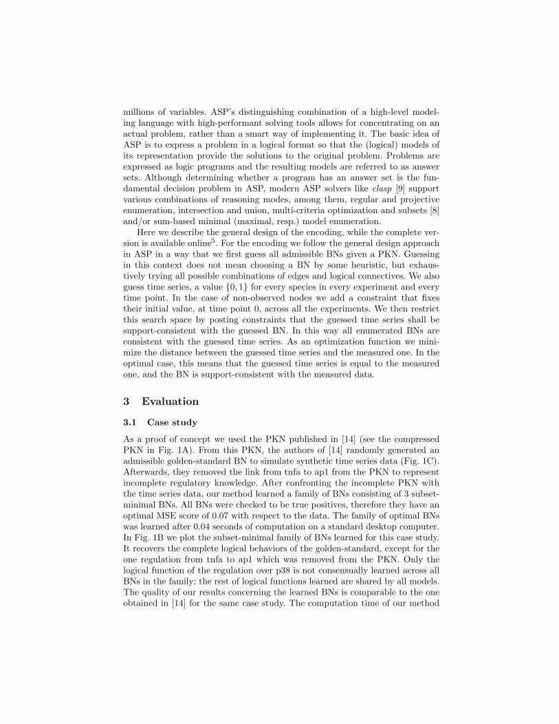
As a proof of concept we used the PKN published in [14] (see the compressedPKN in Fig. 1A). From this PKN, the authors of [14] randomly generated anadmissible golden-standard BN to simulate synthetic time series data (Fig. 1C).Afterwards, they removed the link from tnfa to ap1 from the PKN to representincomplete regulatory knowledge. After confronting the incomplete PKN withthe time series data, our method learned a family of BNs consisting of 3 subset-minimal BNs. All BNs were checked to be true positives, therefore they have anoptimal MSE score of 0.07 with respect to the data. The family of optimal BNswas learned after 0.04 seconds of computation on a standard desktop computer.In Fig. 1B we plot the subset-minimal family of BNs learned for this case study.It recovers the complete logical behaviors of the golden-standard, except for theone regulation from tnfa to ap1 which was removed from the PKN. Only thelogical function of the regulation over p38 is not consensually learned across allBNs in the family; the rest of logical functions learned are shared by all models.The quality of our results concerning the learned BNs is comparable to the oneobtained in [14] for the same case study. The computation time of our method

Fig. 1. (A) Compressed PKN from [14]. Green and red edges indicate activations and inhibi-tions respectively. Colors of the nodes represent the chosen experimental design: green refers toinputs/stimuli, red, to inhibited nodes, and blue, to measured species. (B) Boolean networks (BNs)learned from time series data which are subset-minimal. All BNs predictions have minimal ∆MSEwith respect to the synthetic time series data. A black circle represents a logical AND gate. A numberwritten over an edge represents the frequency of this logical gate or edge with respect to the familyof BNs when the edge is not shared by all BNs. (C) Synthetic time series data used in [14] simulatedusing a BN admissible for the PKN in A. In total 10 experimental conditions were simulated. Redboxes indicate the minimal set of 3 error time-points detected.

improves the one of published methods in a range of 2 to 4 orders of magnitude.Moreover, our method is exhaustive: all logical networks are learned. The fullset of solutions (not only the subset-minimal BNs) was also computed showingone more BN with an OR gate above p38 from tnfa and map3k1.

The method also automatically identified the list of minimal errors in thetime series data, selecting time-points that cannot be explained by the learnedBNs. For the case of all optimal BNs, we found the following 3 errors (see Fig.1C) in all of them. For experiment 10, time-point 10, species p38, the error canbe explained by the noise artificially introduced in the dataset. The predecessorsof p38 are tnfa and egfr, both active in experimental condition 10 (see Fig.1C).The signal of p38 can therefore only increase (or stay the same). However, themeasure of p38 slightly decreases (due to noise) at time-point 10; this generatesan error since the BNs cannot satisfy the data at this particular time-point. Forexperiment 6, time-point 2 and 4, species ap1, the errors can be explained by thefact that one edge (the link from tnfa to ap1) was deleted from the PKN, but waskept to generate the synthetic time series data. All BNs agree on a regulationof p38 and ap1 from map3k1. In experiment 6 tnfa is stimulated and pi3k isinhibited (see Fig. 1C). At time-point 2 the value of map3k1 has to be activated(transition 0 → 1) to justify the activation of ap1. However, since map3k1 isthe only regulator of p38, which is all the experiment at value 0, this cannot beexplained by the BN and generates an error.

3.2 Benchmarks

In this section we evaluate our method for BN identification on synthetic mul-tiplex time series data. Given a PKN, a dataset and a set of inferred BNs, wefocus on two evaluation criteria: the MSE distance of the BNs to the dataset,and the rate of false positives due to our reachability over-approximation.

Synthetic multiplex time series datasets. 10 PKNs were derived by randomlyremoving or adding edges from the compressed PKN published in [14]. For eachPKN we randomly selected 3 golden-standard admissible BNs. Each golden-standard BN was used to generate synthetic time series data by simulating theBN with logic-based ODEs. In total we generated 30 datasets (see appendix Afor details).

MSE computation. Following section 2.3, our method optimizes the MSE of theBNs F to the dataset D up to the reachability over-approximation criteria: if theBN is a true positive, the estimated MSE mse(F,D) is the exact MSE mse(F,D),otherwise the estimated MSE is an under-approximation - the exact MSE maybe larger. Due to the optimization, all the BNs have the same estimated MSE.The value of the estimated MSE can be computed using the equation given insection 2.1 by sampling one BN from the result set with one Boolean trace Xfor each time series T of dataset D such that mse(X,T ) is minimal.

True-positive rate computation. Any BN inferred by our method satisfies thenecessary condition depicted in section 2.2 for producing Boolean traces as closeas possible to a given time series dataset. Verifying that the BN can actuallyreproduce those Boolean traces requires an exhaustive analysis of the dynamicsto ensure the successive reachability of the Boolean states. In the scope of thispaper, we performed such a verification using a model-checking approach. Thepresented experiments have been conducted using the tool NuSMV [5] whichallows an efficient encoding of the dynamics accounting for the range of clampingsettings of the different time series in the dataset5. The true-positive rate eval-uation proceeds by iteratively checking each inferred BN. In the case when theestimated MSE is MSET (section 2.3), the model-checking is performed with re-spect to the binarized time series. Otherwise, we iterate over the closest Booleantraces computed in section 2.3 until a sample is validated by model-checking; ifno such a sample exists, the BN is a false positive.

Results. For each dataset, the model identification has been performed withrespect to the PKNs from which the BNs used for data generation have beenextracted; and with respect to the PKNs where some edges have been deleted sothe BNs used to generate the data are not in the considered domain. Detailedresults are given in appendix B. With the exact PKNs, the estimated MSE isalways the minimum MSET ; moreover, the rate of true positive is 100% in 28benchmark datasets, and above 90% in the 2 others. With the PKNs with deletededges, most of the cases show a very high true positive rate (often 100%) and anestimated MSE close to (often equal to) MSET . Note that for some dataset, notrue positive has been found. For the cases when the estimated MSE is differentfrom MSET , the true positive rate can only be evaluated by sampling Booleantraces close to the time series data. Because of the very high combinatorics ofsuch sampling space, the computation has been aborted after one hour, hence

5 Scripts and data available at http://loicpauleve.name/cmsb15-suppl.tbz2

we cannot guarantee that no true positive exists. When no true positives havebeen identified, the MSE may be under-estimated.

The inference of the subset-minimal solutions for the 30 benchmarks withexact PKNs took less than 2 seconds on average. The performance is similarfor the benchmarks with incomplete PKNs that contained a true positive BNin the result. The number of results varies between 12 and 2640 with the exactPKN and from 2 to 1188 with modified PKNs. Depending on the size and thecomplexity of its dynamics, the model-checking of one BN took between 1s and5 minutes. The full set of solutions (not only the subset-minimal BNs) have alsobeen performed with the exact PKN, showing very similar results and runningtime, with subsequently more results (up to 54,000 BNs, data not shown).

Same experiments have been conducted on the time series generated withnoise (appendix A) but show no difference in the results (data not shown). Thismay indicate that the noise influence may be tempered by the binarization.

3.3 Comparison with inferences using pseudo steady-states

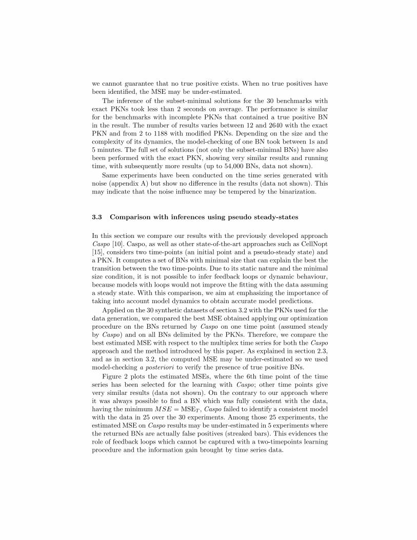
In this section we compare our results with the previously developed approachCaspo [10]. Caspo, as well as other state-of-the-art approaches such as CellNopt[15], considers two time-points (an initial point and a pseudo-steady state) anda PKN. It computes a set of BNs with minimal size that can explain the best thetransition between the two time-points. Due to its static nature and the minimalsize condition, it is not possible to infer feedback loops or dynamic behaviour,because models with loops would not improve the fitting with the data assuminga steady state. With this comparison, we aim at emphasizing the importance oftaking into account model dynamics to obtain accurate model predictions.

Applied on the 30 synthetic datasets of section 3.2 with the PKNs used for thedata generation, we compared the best MSE obtained applying our optimizationprocedure on the BNs returned by Caspo on one time point (assumed steadyby Caspo) and on all BNs delimited by the PKNs. Therefore, we compare thebest estimated MSE with respect to the multiplex time series for both the Caspoapproach and the method introduced by this paper. As explained in section 2.3,and as in section 3.2, the computed MSE may be under-estimated so we usedmodel-checking a posteriori to verify the presence of true positive BNs.

Figure 2 plots the estimated MSEs, where the 6th time point of the timeseries has been selected for the learning with Caspo; other time points givevery similar results (data not shown). On the contrary to our approach whereit was always possible to find a BN which was fully consistent with the data,having the minimum MSE = MSET , Caspo failed to identify a consistent modelwith the data in 25 over the 30 experiments. Among those 25 experiments, theestimated MSE on Caspo results may be under-estimated in 5 experiments wherethe returned BNs are actually false positives (streaked bars). This evidences therole of feedback loops which cannot be captured with a two-timepoints learningprocedure and the information gain brought by time series data.

1.1

1.2

1.3

2.1

2.2

2.3

3.1

3.2

3.3

4.1

4.2

4.3

5.1

5.2

5.3

6.1

6.2

6.3

7.1

7.2

7.3

8.1

8.2

8.3

9.1

9.2

9.3

10.1

10.2

10.3

Dataset

0.00

0.02

0.04

0.06

0.08

0.10

MSE

=

=

==

=

Our method Caspo (true positive) Caspo (false positive)

Fig. 2. Comparing MSE with Caspo for 10 different PKNs with 3 datasets each.“=” indicates equal MSE.

4 Conclusion

We have introduced a procedure based on combinatorial optimization with declar-ative programming approaches and model checking to identify BNs from multi-plex time series data given a prior network structure. To cope with the complex-ity of an exhaustive analysis of BNs dynamics, we defined an abstract semanticsof BNs from which we derived a necessary condition for the satisfaction of suc-cessive reachability properties, induced by the time series data. Our procedureidentifies all the BNs that satisfy this necessary condition with the shortestdistance (in terms of MSE) to the observed experimental data. Because the sat-isfaction criteria for the dynamics is over-approximated, our method may leadto BNs that are false positive, and have an under-estimated MSE. Applied tosynthetic multiplex time series datasets on networks composed of 13 to 17 nodes,the identification of BNs takes only a few seconds and exhibits a very low rateof false positives, showing a remarkable efficiency.

In the present form, we assume that the experimental data is normalized be-tween 0 and 1 and use a discretization threshold at 0.5. Whereas such a settingis relevant for phosphoproteomics data, future work may generalize our opti-mization framework to account for adaptive and multiple discretization levels.Moreover, application to larger networks should be considered, although few ofsuch data are currently available, and generating synthetic data with sufficientdiscriminant power may be challenging.

Because our identification method can be exhaustive, the framework we pro-pose is suited for the complete Thomas parameters identification for BNs fromincomplete time series data [13,6].Thanks to our abstract semantics, our methodis able to filter out very efficiently a large number of candidate BNs without acostly exact model-checking, which is postponed to the validation of the results.In that way, future work may further explore the combination of dynamics over-

approximations with model-checking approaches to provide scalable and exactinference of BNs from time series data.

References

1. L. G. Alexopoulos, J. Saez-Rodriguez, B. Cosgrove, D. A. Lauffenburger, andP. Sorger. Networks inferred from biochemical data reveal profound differencesin toll-like receptor and inflammatory signaling between normal and transformedhepatocytes. Molecular & Cellular Proteomics, 9(9):1849–1865, 2010.

2. J. Aracena, E. Goles, A. Moreira, and L. Salinas. On the robustness of updateschedules in boolean networks. Biosystems, 97(1):1 – 8, 2009.

3. C. Baral. Knowledge Representation, Reasoning and Declarative Problem Solving.Cambridge University Press, 2003.

4. N. Berestovsky and L. Nakhleh. An evaluation of methods for inferring booleannetworks from time-series data. PLoS ONE, 8(6):e66031, 2013.

5. A. Cimatti, E. Clarke, E. Giunchiglia, F. Giunchiglia, M. Pistore, M. Roveri, R. Se-bastiani, and A. Tacchella. NuSMV 2: An opensource tool for symbolic modelchecking. In Computer Aided Verification, volume 2404 of LNCS, pages 241–268.Springer Berlin / Heidelberg, 2002.

6. E. Gallet, M. Manceny, P. Le Gall, and P. Ballarini. An ltl model checking approachfor biological parameter inference. In Formal Methods and Software Engineering,volume 8829 of LNCS, pages 155–170. Springer, 2014.

7. M. Gebser, R. Kaminski, B. Kaufmann, and T. Schaub. Answer Set Solving inPractice. Synthesis Lectures on Artificial Intelligence and Machine Learning. Mor-gan and Claypool Publishers, 2012.

8. M. Gebser, B. Kaufmann, R. Otero, J. Romero, T. Schaub, and P. Wanko. Domain-specific heuristics in answer set programming. In Proceedings of the 27th NationalConference on Artificial Intelligence (AAAI’13), pages 350–356. AAAI Press, 2013.

9. M. Gebser, B. Kaufmann, and T. Schaub. Multi-threaded ASP solving with clasp.Theory and Practice of Logic Programming, 12(4-5):525–545, 2012.

10. C. Guziolowski, S. Videla, F. Eduati, S. Thiele, T. Cokelaer, A. Siegel, and J. Saez-Rodriguez. Exhaustively characterizing feasible logic models of a signaling networkusing answer set programming. Bioinformatics, 29(18):2320–2326, 2013.

11. D. Harel, O. Kupferman, and M. Y. Vardi. On the complexity of verifying concur-rent transition systems. Information and Computation, 173(2):143 – 161, 2002.

12. S. Kauffman. Metabolic stability and epigenesis in randomly constructed geneticnets. Journal of Theoretical Biology, 22(3):437–467, 1969.

13. H. Klarner, A. Streck, D. Safranek, J. Kolcak, and H. Siebert. Parameter iden-tification and model ranking of thomas networks. In Computational Methods inSystems Biology, pages 207–226. Springer Berlin Heidelberg, 2012.

14. A. MacNamara, C. Terfve, D. Henriques, B. P. Bernabe, and J. Saez-Rodriguez.State-time spectrum of signal transduction logic models. Phys Biol, 9(4), 2012.

15. J. Saez-Rodriguez, L. G. Alexopoulos, J. Epperlein, R. Samaga, D. A. Lauffen-burger, S. Klamt, and P. K. Sorger. Discrete logic modelling as a means to linkprotein signalling networks with functional analysis of mammalian signal trans-duction. Molecular Systems Biology, 5(331), 2009.

16. R. Wang, A. Saadatpour, and R. Albert. Boolean modeling in systems biology: anoverview of methodology and applications. Phys Biol, 9(5), 2012.

A Synthetic data generation

We produced a family of 10 PKNs derived by randomly removing or addingedges to the compressed PKN published in [14]. The 10 PKNs had a numberof nodes and edges in the range of 13-17 and 16-22 respectively. For each PKNwe generated its expanded version, that is, a super-structure of BNs in whichall nodes of the PKN are associated to their predecessors in the graph usingall possible combinations of AND and OR gates. The expansion method wasintroduced in [15].

From this super-structure we selected 3 golden-standard BNs with a numberof AND gates lower or equal to 1, 3, and 5 respectively. The AND gates werechosen randomly, however preserving that all nodes are connected to the inputnodes (signaling or stimuli) of the experimental design.

Afterwards, each golden-standard BN was used to generate synthetic time-series data by simulating the BN with logic-based ordinary differential equationsand arbitrary parameters based on the experimental design used in [14]. Wegenerated synthetic expression values of 6 species (ap1, erk, gsk3, nfkb, p38and raf1) across 16 time-points {0, 2, 4, 6, . . . , 30} in 10 experimental clampingsettings which were either stimulation of the inputs (egf, tnfa) or inhibition ofinhibitors (pi3k, raf1). In total we generated 30 time-series synthetic datasets.

For the BN learning process we used synthetic datasets with or without noise,as well as altered PKNs by removing one or two edges from the 10 PKNs. Thenoise of the datasets was uniformly distributed between −0.5 and 0.5 and addedto the values contained in the dataframe (for each combination of species andtime/experiment). The new values were X = X + noise(−.5, .5) ∗ dr, where drwas fixed to 0.1 and 0.2. To generate the synthetic data we used the R packageCNORode and the Python package cellnopt.wrapper.

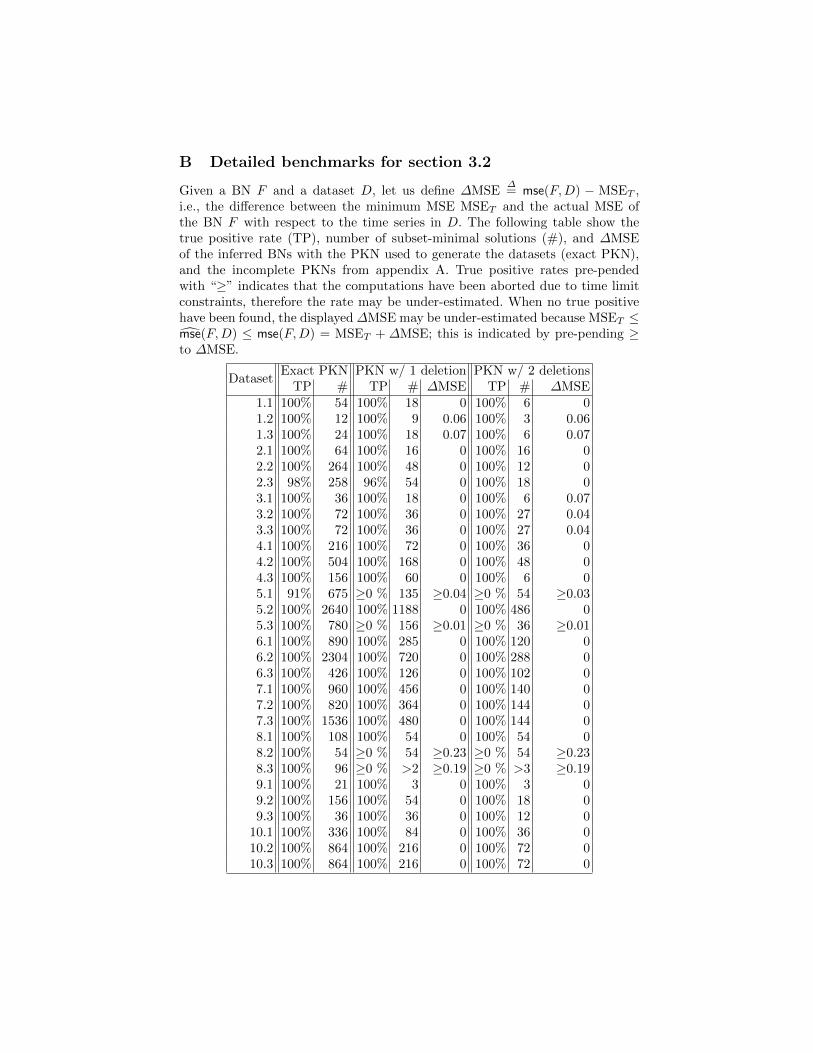
B Detailed benchmarks for section 3.2

Given a BN F and a dataset D, let us define ∆MSE∆= mse(F,D) − MSET ,

i.e., the difference between the minimum MSE MSET and the actual MSE ofthe BN F with respect to the time series in D. The following table show thetrue positive rate (TP), number of subset-minimal solutions (#), and ∆MSEof the inferred BNs with the PKN used to generate the datasets (exact PKN),and the incomplete PKNs from appendix A. True positive rates pre-pendedwith “≥” indicates that the computations have been aborted due to time limitconstraints, therefore the rate may be under-estimated. When no true positivehave been found, the displayed ∆MSE may be under-estimated because MSET ≤mse(F,D) ≤ mse(F,D) = MSET + ∆MSE; this is indicated by pre-pending ≥to ∆MSE.

DatasetExact PKN PKN w/ 1 deletion PKN w/ 2 deletions

TP # TP # ∆MSE TP # ∆MSE1.1 100% 54 100% 18 0 100% 6 01.2 100% 12 100% 9 0.06 100% 3 0.061.3 100% 24 100% 18 0.07 100% 6 0.072.1 100% 64 100% 16 0 100% 16 02.2 100% 264 100% 48 0 100% 12 02.3 98% 258 96% 54 0 100% 18 03.1 100% 36 100% 18 0 100% 6 0.073.2 100% 72 100% 36 0 100% 27 0.043.3 100% 72 100% 36 0 100% 27 0.044.1 100% 216 100% 72 0 100% 36 04.2 100% 504 100% 168 0 100% 48 04.3 100% 156 100% 60 0 100% 6 05.1 91% 675 ≥0 % 135 ≥0.04 ≥0 % 54 ≥0.035.2 100% 2640 100% 1188 0 100% 486 05.3 100% 780 ≥0 % 156 ≥0.01 ≥0 % 36 ≥0.016.1 100% 890 100% 285 0 100% 120 06.2 100% 2304 100% 720 0 100% 288 06.3 100% 426 100% 126 0 100% 102 07.1 100% 960 100% 456 0 100% 140 07.2 100% 820 100% 364 0 100% 144 07.3 100% 1536 100% 480 0 100% 144 08.1 100% 108 100% 54 0 100% 54 08.2 100% 54 ≥0 % 54 ≥0.23 ≥0 % 54 ≥0.238.3 100% 96 ≥0 % >2 ≥0.19 ≥0 % >3 ≥0.199.1 100% 21 100% 3 0 100% 3 09.2 100% 156 100% 54 0 100% 18 09.3 100% 36 100% 36 0 100% 12 0

10.1 100% 336 100% 84 0 100% 36 010.2 100% 864 100% 216 0 100% 72 010.3 100% 864 100% 216 0 100% 72 0