boiling of refrigerants on enhanced ...7515/fulltext01.pdftrita refr report no 03/37 issn 1102-0245...
TRANSCRIPT

Trita REFR Report No 03/37
ISSN 1102-0245 ISRN KTH/REFR/R03/37 SE
BOILING OF REFRIGERANTS ON ENHANCED SURFACES
AND
BOILING OF NANOFLUIDS
Sanjeeva Witharana
Licentiate Thesis
May 2003
Department of Energy Technology
Division of Applied Thermodynamics and Refrigeration
The Royal Institute of Technology
Stockholm, Sweden

Copyright Sanjeeva Witharana 2003
Trita REFR Report No 03/37
ISSN 1102-0245
ISRN KTH/REFR/R03/37 SE

Acknowledgements Björn Palm, Professor, for guiding and supervising my work Eric Granryd, Professor Emeritus, for recruiting me as a graduate student The State of Sweden, for financing this project Mamoun Muhammed, Professor, for exposing me to nanotechnology Yu Zhang, Senior Researcher, for occasional supervision Muhammet Toprak, for cooperating in the project work Salam, Nalin, for helping in various ways Bosse, Benny, for assisting in the workshop Inga, for many reasons Birger & Tony, for attending to computer matters Every individual in the department of energy technology, and, the nanosynthesis laboratory, for being friendly & caring
Sanjeeva Witharana Stockholm 2003-05

dedicated to My motherland Sri Lanka

TABLE OF CONTENTS
INTRODUCTION v
PART I
Chapter 1: BOILING AND BUBBLE NUCLEATION
1.1 Introduction to Pool Boiling 1 1.11 The Natural Convection Region 1.12 The Nucleate Boiling Region
1.2 Introduction to Flow Boiling 4 1.3 The mechanism of Bubble Nucleation 6 1.4 Correlations for Heat Transfer Coefficients in Nucleate Boiling 9
1.4.1 Nucleate Pool Boiling 1.4.2 Flow Boiling
Chapter 2: BOILING ENHANCEMENT
2.1 The motive for Boiling Enhancement 15 2.2 Enhancement Techniques – A general overview 16 2.3 Boiling on Enhanced Surfaces 18 2.4 The degree of Enhancement – Early findings 19
2.4.1 Structured Surfaces 2.4.2 Coated Surfaces 2.4.3 Performance comparison-Structured and Coated surfaces
2.5 Parameters that influence the degree of Enhancement 24 2.5.1 The shape and the geometry of cavities 2.5.2 The nucleation site density 2.5.3 Particle size, coating thickness, and the porosity 2.5.4 The base surface thermal conductivity 2.5.5 Some more observations
2.6 Models and Correlations for Structured surfaces 37 2.7 Models and Correlations for Coated surfaces 48 2.8 Boiling Enhancement – Goal of the present investigation 55
Chapter 3: THE EXPERIMENTAL SET UP AND PROCEDURE
3.1 The sample holder 57 3.2 Sample Manufacture 59
3.2.1 Mechanically treated surfaces 3.2.2 Electro-chemically etched surfaces
3.3 Surface preparation by Electro-Chemical etching 61 3.3.1 Instruments 3.3.2 Procedure
3.4 Surface preparation by Electro-deposition 64

Sanjeeva Witharana: Boiling of refrigerants on enhanced surfaces and Boiling of nanofluids
ii
3.5 Boiling, regulation and data collection 66 3.5.1 Pool boiling 3.5.2 Regulation and Data collection
3.6 Calculations 69 3.6.1 Pore depth 3.6.2 Heat loss through the insulation 3.6.3 Surface temperature 3.6.4 Heat transfer coefficient
3.7 Problems from design to operation 72 3.7.1 Choice of a Heater 3.7.2 The Bonding mechanism for the Sample and the Heater 3.7.3 Temperature measurements
Chapter 4: EXPERIMENTAL RESULTS
4.1 Samples and Test conditions 79 4.1.1 Pore diameter, Pore depth and the Porosity 4.2 Presentation and discussion of results 81 4.2.1 Wall superheat and heat transfer coefficient
4.2.2 Evaluation of results 4.2.3 Oil tests 4.2.4 Boiling hysteresis
4.3 Summary of results 92
Chapter 5: CONCLUSION AND FUTURE WORK 93 References - Part I 95
PART II
Chapter 6: INTRODUCTION TO NANOFLUIDS
6.1 Introduction to Nanotechnology 105 6.2 Nanoparticles 106 6.3 Properties of Nanoparticles 106 6.4 Extraction of Nanoparticles 107 6.5 Introduction to Nanofluids 108
6.5.1 State-of- the art 6.5.2 Present investigation
Chapter 7: EXPERIMENTS WITH NANOFLUIDS
7.1 Production of nanoparticles 115 7.2 The Experimental set-up and test conditions 116 7.3 Test procedure 118 7.4 Calculations 119

Table of contents
iii
7.5 Experimental results 119 7.5.1 Results from water based nanofluids 7.5.2 Results from ethylene glycol based nanofluids
7.6 Summary of results 122 7.7 Concluding remarks and Discussion 122 7.8 Future work 123
References – Part II 125
List of Symbols 127 List of Tables 129 List of Figures 131

INTRODUCTION
Background to the topic
We have heard people talking of energy crisis. Some of these people try to find
solutions, while some of them try to find offenders. A third group, in fact, keep silent.
We, the energy engineers belong to the first category. Among us, there are two sub-
groups operating, one investigating efficient extraction methods from energy sources,
while the other developing techniques for efficient energy usage. I will locate myself
in the first group. Nevertheless, we altogether, have been taught of the first law of
thermodynamics. It says, energy can neither be created nor destroyed. It is all about
conversion from one kind of energy to another. A typical example is the potential
energy of a waterfall, turning to the mechanical energy of a turbine, turning to the
electric energy in a generator. We call it hydropower. But, the cycle doesn’t stop
there. Whatever use you make of electricity comes thereafter. From the first law, we
know that the energy does not leave this world. If so, why are we conservative in
usage? The answer is simple. We have to pay for it. We, as energy engineers, are duty
bound with ambition to reduce your electricity bills, while caring for the environment.
Refrigerating and air conditioning machines supply cold where it is needed. In cold
climates, like in Sweden, people use heat pumps to keep their dwellings and
workplaces warm. Technically, the refrigerators and heat pumps work on the same
principle. These units as a whole, consume large amounts of energy, let it be
electrical, oil, gas, or renewable. Individually, the user is billed for what he consumes.
This project is aimed at improving the energy efficiency of refrigerating (and heat
pumping) machines, by improving the efficiency of the heat exchangers within these
units. Let us look at the cost benefits of such an improvement done on a refrigerator.
The Carnot refrigeration cycle is represented on a conventional temperature-entropy
(T-S) diagram in the way shown in figure 1. If the cold space is a room, for example a
cold room, then Tsource will be the room temperature. If the warm side of this
refrigerator is placed outside the room, for example in the outside air, then Tsink will
be the air temperature. The refrigerant in the low temperature heat exchanger (at T2)
absorbs heat from the source and is pumped to the high temperature heat exchanger
(operating at T1) by a compressor.

Sanjeeva Witharana: Boiling of refrigerants on enhanced surfaces and Boiling of nanofluids
vi
T
S
Tsource
Tsink
T2
T1
∆S
Figure 1: The ideal vapour compression cycle
Let the cooling capacity of the low temperature heat exchanger be 2Q& , and the
electrical input to the compressor be E& . Then, the efficiency parameter for this
refrigerator COP2 (coefficient of performance) can be written as,
E
QCOP
&
&2
2 = 1
In temperature terms and under certain assumptions, the equation 1 is re-written as:
21
22
TT
TCOP
−= 2
From 1 and 2, the compressor electrical consumption then takes the form of,
( )2
212 .
T
TTQE
−=&
& 3
If we can lift T2 by few degrees towards T1, what will be the effect on E& ? Consider
two cases with same ambient conditions. In the first case, let us assume T2 =10°C,
while in the second case, T2 =15°C. In two cases, we further assume that T1=40°C
and 2Q& does not change. Now, from equation 3 we get, )/( III EE && = 0.82. Hence, we
have been able to save compressor power consumption by 18%, by reducing the
temperature difference between the condenser and the evaporator (T1 – T2) by 5°C.
Take United States for a case study. They claim to spend over $80 billion on energy
for air conditioning and refrigeration [Eastman et al. 2002]. A modest 10% saving in
these cooling machines will return $8 billion saving in money.

Introduction
vii
Another advantage is that, as the energy efficiency increases, the units become
smaller in size and lighter in weight.
My objective in this project is specifically to reduce the temperature difference as said
above. The approach I take in this regard is such that we are going to design
evaporators, which operate at temperatures as close as possible to the source
temperature.
Structure of the thesis
I have formulated this thesis in two parts, the first part on Boiling of Refrigerants on
Enhanced surfaces, and the second part on Boiling of Nanofluids. The part on boiling
on enhanced surfaces deals straight with the topic from the beginning, under the
assumption that you are fairly exposed to the matured science of boiling. However,
the topic of nanofluids is likely to be new to you, like to many of us, to a great extent.
Therefore I start the second part of the thesis with a broad introduction to the
nanotechnology. This discussion will gradually take you to the experimental work.
Part I - Boiling of Refrigerants on Enhanced surfaces
The aim of the first part of this report is to present an investigation into finding an
enhanced boiling surface that would efficiently transfer heat to a colder refrigerant.
The techniques of boiling enhancement have come under rigorous investigation since
1930’s while the science of boiling reported in literature itself is bearing an even
longer history, running for more than a century of years.
R.L. Webb [1983] and A.E. Bergles [1991] respectively documented the number of
U.S. patents and journal publications related to the enhancement technology over the
years. Citations on heat transfer augmentation, as shown in figure 2, started a rapid
growth until the 1990’s. During this period of time, prominent names in this field
were W.Nakayama, A.E. Bergles, R.L. Webb, and their co-workers.
Sanjeeva Witharana: Boiling of refrigerants on enhanced surfaces and Boiling of nanofluids
viii
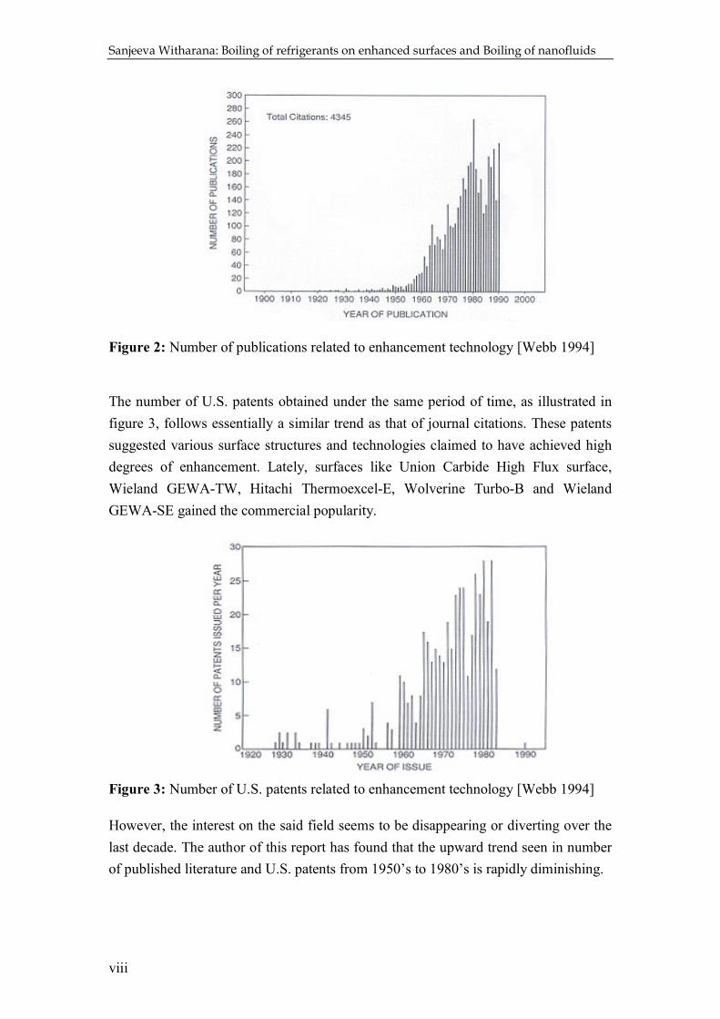
Figure 2: Number of publications related to enhancement technology [Webb 1994]
The number of U.S. patents obtained under the same period of time, as illustrated in
figure 3, follows essentially a similar trend as that of journal citations. These patents
suggested various surface structures and technologies claimed to have achieved high
degrees of enhancement. Lately, surfaces like Union Carbide High Flux surface,
Wieland GEWA-TW, Hitachi Thermoexcel-E, Wolverine Turbo-B and Wieland
GEWA-SE gained the commercial popularity.
Figure 3: Number of U.S. patents related to enhancement technology [Webb 1994]
However, the interest on the said field seems to be disappearing or diverting over the
last decade. The author of this report has found that the upward trend seen in number
of published literature and U.S. patents from 1950’s to 1980’s is rapidly diminishing.

Introduction
ix
While mechanically fabricated enhanced surfaces are holding on to its grip somewhat,
porous boiling surfaces have failed to document any major commercial
breakthroughs. Yet encouragingly, porous boiling surfaces are witnessed to be gaining
grounds in electronic cooling applications.
The thesis starts with chapter 1, devoted to explain boiling fundamentals. The
knowledge of boiling fundamentals, like bubble nucleation and growth, is clearly the
key to understand the boiling mechanism on enhanced surfaces. In view of that, the
chapter 1 deals with the basics of pool boiling, flow boiling and bubble nucleation.
Finally, some widely used correlations for pool boiling and flow boiling are
introduced.
Chapter 2 is a comprehensive literature survey on the state-of-the art of enhanced
surfaces. It contains the history and the development of the topic, the surface
geometries, the predictive models and experimental results. A comparison of
performance of structured and porous surfaces is also presented wherever possible.
Moreover, the much-pronounced areas like hysteresis, aging, and the effect of oil in
the refrigerant are also treated. The chapter is wrapped up by statement of the goal of
the present work.
The experimental set up and the test samples are introduced in chapter 3. The boiling
chamber and the data collection system, the heater arrangement, and the surface
preparation are described in detail. The scanning electron microscopy (SEM) as well
as light optical microscopy (LOM) pictures provide a close view of the test surfaces.
The equations for the chemical reactions in etching and deposition, and heat transfer
are also stated. Towards the end, the technical and operational problems we faced
from the start of the project are shared with you.
Chapter 4 is exclusively dealing with the experimental results. The experiments were
conducted with pure Refrigerant-134a, and that mixed with synthetic refrigeration oil.
A comparison of the experimental data on the newly found surfaces with those of
traditional surfaces is presented in this chapter.
A general conclusion of the experimental work is drawn in chapter 5. In addition, a
review of the initial goal, and directions for the future work are mentioned. Part 1 of
the thesis concludes with chapter 5.

Sanjeeva Witharana: Boiling of refrigerants on enhanced surfaces and Boiling of nanofluids
x
Part II – Boiling of Nanofluids
Nanotechnology is the science of working with nanosized particles. A nanometer is
one-billionth of a meter, or about 100,000 times smaller than the width of a human
hair. At nanoscale, the properties of a substance significantly differ from that of the
bulk material. Due to this interesting phenomenon, the nanotechnology has been
considered as a tool to improve performance of old materials, or to design new
materials. The physics and chemistry of nanoscale systems has advanced rapidly over
the last few years. Since nanotechnology is a generic technology, it also has the
potential to impact on a wide range of industrial sectors, from chemicals to
electronics, from sensors to advanced materials. One of its applications is in the area
of refrigeration.
Nanofluids, which are suspensions of nanoparticles in liquids, have displayed higher
thermal conductivities and heat transfer coefficients than their base fluids. It has been
reported approximately 20% improvement in effective thermal conductivity when
5 vol.% CuO nanoparticles are added to water [Eastman et al. 1999]. The effective
thermal conductivity of Ethylene Glycol, which is widely used as a secondary
refrigerant, increased as much as up to 40% for a nanofluid consisting of Ethylene
Glycol with approximately 0.3 vol.% Cu nanoparticles [Eastman et al. 2001].
Chapter 6 of this thesis starts giving a general outline of the nanotechnology and its
applications to the reader. Despite the fact that the nanotechnology is largely in the
experimental scale at the moment, it has shown superiority in some practical
applications. Through the general discussion, the reader is taken to the topic of
nanofluids.
Chapter 7 serves the purpose of presenting and discussing experimental results on
boiling of nanofluids. Some of these results, which are not presently published
elsewhere, of course are expected to draw the curiosity of the audience. Part II as well
as this thesis ends with chapter 7.

PART I
BOILING OF REFRIGERANTS ON ENHANCED SURFACES

Chapter 1
BOILING AND BUBBLE NUCLEATION
Boiling is a means of transferring heat from a hot surface to a relatively cold fluid,
which is in contact with the surface. Boiling of liquids on surfaces may be analysed
under two categories, viz., pool boiling and flow boiling, where the latter is also
referred to as convective boiling in some literature. This chapter begins with
introduction to pool boiling. Different regimes of pool boiling are discussed with the
help of the boiling curve. Primary attention is paid on nucleate boiling regime, which
the coming chapters are based upon. The flow boiling is also discussed as a concept.
Bubble nucleation is addressed under three conditions for nucleation. And finally,
some famous correlations for pool boiling and flow boiling picked from the literature,
are also mentioned.
1.1 Introduction to Pool boiling
Pool boiling is a condition where boiling occurs from a heated surface submerged in a
large volume of stagnant liquid. This liquid may be at its boiling point in which case
the process is called saturated pool boiling or below its boiling point, in which case it
is called subcooled pool boiling.
Pool boiling heat transfer is easily explained by referring to the pool boiling curve.
The pool boiling cure for a particular surface-liquid combination represents the
functional dependence of the heat flux leaving the hot surface on the temperature
difference between the hot surface and the saturation temperature. This temperature
difference is traditionally known as the wall superheat. Nukiyama [1934] is said to be
the first to publish a pool boiling curve based on results from his well-known
experiment, power-controlled heating of saturated water at atmospheric pressure.
Figure 1.1 shows the boiling curve for pool boiling of water at atmospheric pressure.
Heater surface temperature is plotted along the abscissa while the heat flux passing
from the heated wall into the fluid is plotted along the ordinate.

Sanjeeva Witharana: Boiling of refrigerants on Enhanced surfaces
2
Figure 1.1: Pool boiling of water at atmospheric pressure [Collier and Thome 1994]
The boiling curve can be conveniently analysed in four different regions, namely, the
natural convection AB, the nucleate pool boiling CB′ , the transition DE, and the film
boiling EF regions. In the context of this report, it would be sufficient to treat the
natural convection region and nucleate pool boiling region in detail.
1.11 The Natural Convection Region (AB)
As the temperature of the heater is gradually increased from below the saturation
temperature (corresponding to the liquid pressure), first to come into effect are the
natural convection currents. Natural convection, caused by the temperature gradients
set up in the pool, removes the heat from the heating surface to the free liquid surface
and then by evaporation to the vapour space. As the surface temperature is increased
passing the saturation temperature, at a certain point, bubbles would form on the
surface, indicating the beginning of the nucleate boiling region.

Chapter 1: Boiling and bubble nucleation
3
1.12 The Nucleate Boiling Region ( CB′ )
The nucleate boiling region is characterised by bubble formation on the heating
surface. The wall temperature must reach a minimum value (shown by B in this case)
above saturation temperature of the liquid, in order for a bubble to appear. The
process of bubble formation, technically termed as vapour nucleation, which gives
birth to the phenomena of nucleate boiling, is the most important part of boiling heat
transfer analysis presented in this report.
The curve has a steep slope in the region CB′ compared with that in AB. It indicates
that a small step-increase in wall superheat in CB′ region will result in a larger
increase in heat removal from the surface. For the nucleate boiling region, the
relationship between the wall superheat Tw-Ts, and the surface heat flux q& , is written
in the form of an empirical power law relationship,
nsw qCTT &.=− 1.1
Where, C and n are constants depending upon the physical properties of the liquid,
vapour, and upon the nucleation properties of the surface. The value for index n is
approximately 0.4.
Rohsenow [1973] approximates heat transfer in nucleate boiling on a planer surface
to,
( )3
sw TTq −≈& 1.2
While Tong [1965] suggests the index 3 in Rohsenow [1973]’s correlation may vary
between 2 to 5.
Nucleate boiling is a well-recognised means for removing high heat loads from a
device while maintaining relatively low surface temperatures. Its inherent ability to
achieve high heat removal rates at relatively low wall superheats has earned nucleate
boiling the significance it has been enjoying, in particular, throughout the last few
decades.
It has been found that the high heat transfer rate in nucleate boiling is caused by the
formation and transportation of vapour bubbles. Hsu and Graham [1986] explains this
as a combined action of:
• Thin film evaporation of the superheated liquid surrounding the growing
bubble. Heat is transported in the form of latent heat.

Sanjeeva Witharana: Boiling of refrigerants on Enhanced surfaces
4
• Departing bubble stripping the thermal boundary layer on the surface thus
paving the way for the surrounding liquid to flush into that space. Heat is
transported in the form of sensible heat in the superheated liquid.
• Escaping bubbles agitating the liquid pool. Such agitation action would make
turbulence in the liquid pool, inducing a forced convection heat transfer
process. Heat is transported in the form of sensible heat in the superheated
liquid.
However, an exact account of the contributions from each of these components is yet
to be found.
1.2 Introduction to Flow boiling
As the name implies by itself, flow boiling is discussed in situations where a liquid is
circulated by using external means, such as a pump. Flow boiling is frequently
witnessed in heat transfer arrangements in tubes and ducts.
Illustrated in figures 1.2 and 1.3 are the flow regimes and corresponding heat transfer
regimes in flow boiling inside a vertical tube and in a horizontal tube. In both cases,
the tubes are heated from outside.

Chapter 1: Boiling and bubble nucleation
5
Figures 1.2: Flow boiling in a vertical tube [Du Teaux 1998]
Figure 1.3: Flow boiling in a horizontal tube [Du Teaux 1998]
Figure 1.4 shows the influence of forced evaporation and nucleate boiling regimes on
convective vaporization as the vapour fraction increases along the tube. The influence
of nucleate boiling is decreasing due to a reduced driving force. The forced
evaporation contribution is increasing as the vapour fraction is increasing.

Sanjeeva Witharana: Boiling of refrigerants on Enhanced surfaces
6
Figure 1.4: Influence of vapour fraction on heat transfer [Melin 1996]
1.3 The mechanism of Bubble nucleation
Nucleate boiling involves two separate processes; the formation of bubbles
(nucleation), and the subsequent growth and motion of bubbles. Most of the proposed
theories assume the existence of nuclei from which bubbles originate but the exact
nature of the origin of these nuclei remains to be fully explained.
We consider three types of different idealised conditions of nucleation:
I. Pure liquid; no suspended foreign matter; heated by radiation, cool smooth
walls so that no nucleation occurs at walls
II. Liquid with submicroscopic nonwettable material that contains permanent
gas pockets from which bubble nuclei emerge on volume heating; no
nucleation at cool, smooth walls
III. Heating at wall with surface cavities containing gas/vapour.
Nucleation in pure liquids, type I, occurs as a result of thermal fluctuations occurring
in a metastable liquid. Metastable state of a pure liquid could be described using a
conventional p-v-t diagram for a single pure substance.
Consider a conventional pressure-volume diagram shown in figure 1.5. The liquid at
point A, isothermally expanded, would normally result boiling at Pressure Pb at point
B. However if the liquid is of high purity and the container is very clean and does not
react with the liquid, it is possible to proceed as a liquid down to point C. The
portions BC and EF in figure 1.5 represent metastable states; superheated liquid and
subcooled vapour. This process of vapour formation in a metastable liquid is also

Chapter 1: Boiling and bubble nucleation
7
known as homogeneous nucleation. The rate of homogeneous nucleation increases
rapidly with the degree of liquid superheat. However, probability of forming vapour
by this process is reportedly low.
Figure 1.5: Pressure-Volume diagram for a fluid [Van stralen and Cole 1979]
Nucleation of type II can be described as gas or vapour pockets already present in the
liquid. This method of vapour generation from pre-existing nuclei is also referred to
as heterogeneous nucleation. For such a bubble to grow, a relatively low vapour
superheat would be sufficient.
The third type is known as the nucleation at solid surfaces. Surfaces those appear to
be smooth to the naked eye are in fact, not smooth in microscopic view. Grooves and
cavities in such surfaces act as nucleation sites for bubbles to grow and subsequently
to depart from the surface. The following text would be aimed at explaining the
process of bubble nucleation at solid surfaces to certain detail.
Free energy of formation of a nucleus of radius r, ∆G(r), can be determined from
( )lv PPrrrG −−=∆ 32
3
44)( πσπ 1.3
Where, σ is the surface tension of the liquid-vapour interface, and, (Pv-Pl) is the
pressure difference between the vapour in the bubble and the surrounding liquid.

Sanjeeva Witharana: Boiling of refrigerants on Enhanced surfaces
8
Bankoff [1957] analytically demonstrated that, in the presence of a flat surface, like
the solid wall mentioned here, the ∆G(r) may reduce by a factor Φ given by:
( )4
.22 2θθθ SinCosCos ++=Φ 1.4
Where θ is defined as the contact angle between surface and the liquid measured
through the liquid as shown in figure 1.6.
For a completely wetting surface, θ = 0, Φ = 1 and there is no reduction of the free
energy of formation. For a completely non-wetting surface, θ = 180, Φ = 0 and no
superheat would be required for nucleation at the surface. In most cases, the values for
θ have been observed falling in-between 0° and 90° thus Φ ranging from 1 to 0.5. The
consequent reduction in ∆G(r) will lead to a reduction in the necessary superheat, Tv-
Tl, for bubble nucleation. However, this much of superheat is too small to initiate
homogeneous nucleation. Then the question arises how a bubble could form at this
low superheat. Consequently, people began to investigate the relationship between the
surface conditions and the nucleation superheat.
Figure 1.6 shows liquid-surface interaction in macroscopic view. The definition for
contact angle is shown in (a), while (b), (C) and (d) of figure 1.6 illustrates the
possible liquid vapour interfaces in cavities. Symbolised by β is the included angle of
the cavity.
Figure 1.6: Liquid-surface interaction [Collier and Thome 1994]
Any cavity on a surface should result in belong to either of the liquid-vapour
interfaces shown by (c) or (d). As the temperature of the surface is increased gradually
above the saturation temperature of the liquid, the vapour fronts in both (c) and (d)
will rapidly travel towards the mouth of the cavity, and then takes a convex shape into
the liquid, as illustrated in figure 1.7.

Chapter 1: Boiling and bubble nucleation
9
Figure 1.7: Advancing vapour front [Collier and Thome 1994]
Since the vapour established a convex boundary in the liquid indicated by stage 4 in
the figure, the surrounding superheated liquid starts to evaporate into the vapour space
tending the bubble to grow on surface as well as in the liquid. Bubble expanding on
the surface, will cover more cavities in the neighbourhood filling them with vapour.
Hence, all that is needed for normal boiling is one active nucleating cavity of vapour
or gas. When the surface temperature is raised above the saturation temperature to
nucleate one cavity, the bubble growing at the surface usually remain attached long
enough to cover a number of neighbouring cavities, filling them with vapour, and
causing them to become vapour-nucleating cavities. Once nucleation has been
accomplished, the resulting bubbles, by one means or another, produce dramatic
decreases in temperature difference.
1.4 Correlations for heat transfer coefficients in nucleate boiling
The researchers over the years have been trying to find an expression for nucleate
boiling as a correlation of Nusselt, Reynold’s and Prantle numbers. The common
appearance of this expression was in the form of
nmCNu PrRe= 1.7
Then, their task was to find values for the constant C, and the exponents m and n.
Outlined in the forthcoming discussion are a selection of work, which in this author’s
view, have largely contributed to widen the knowledge of nucleate boiling.

Sanjeeva Witharana: Boiling of refrigerants on Enhanced surfaces
10
1.41 Nucleate Pool Boiling
From literature review, it was found that Rohsenow [1952]’s correlation to predict the
heat transfer coefficient in nucleate boiling was among the first of such kind to gain
recognition. Similar to single-phase convection process, in nucleate boiling too, the
heat leaving the surface first reaches the adjacent liquid layer. According to
Rohsenow, the higher heat transfer rates associated with the latter case were caused
by the bubbles departing from the surface. The resulting correlation takes the shape
of,
( ) ml
n
sll
bb
Ck
dhNu −−== Pr.Re.
1. 1 1.8
Where db is the bubble departure diameter, and, Csl as well as m and n are constants
depending on different nucleation properties of a particular liquid-surface
combination, while the Reynolds number was expressed using the superficial liquid
velocity towards the surface, given by,
( ) l
l
vllfg gh
q
µρ
ρρσ
ρ.
..Re
21
−
=&
1.9
Forster and Zuber [1955] suggested a micro convection model for nucleate boiling,
l
lb
RR
µρ &...2
Re = 1.10
( ) llwl
bb
kTT
Rq
k
dhNu
.
.2..
−==
& 1.11
Where, bubble growth radius R, the velocity of the interface .
R , and Ja are given by,
( ) 21
... tJaR lαπ= 1.12
21
.4
..
=
tJaR lαπ& 1.13
( )fgv
slpl
h
TTCJa
.
..
ρρ −
= ∞ 1.14
However, the applicability of this model imposes limits when it comes to nucleate
pool boiling. Also, it has been found that the Nub for nucleate pool boiling determined

Chapter 1: Boiling and bubble nucleation
11
from experimental results, and the Nub predicted by the model has shown better
agreement when (Tw-Tl) is replaced with (Tw-Ts).
Ishibashi [1969] presented a fairy simple correlation between the heat transfer
coefficient and the heat flux, for boiling of saturated water in narrow spaces,
nqh &∝ 1.15
With index n is set to 2/3. Later Stephan [1992] suggested values around 0.6 to 0.8 for
n.
Stephan and Abdelsalam [1980] presented correlations recommended for several
classes of fluids including water, organics, refrigerants and cryogens. For refrigerants
they proposed,
533.0
581.0745.0
Pr...
...207 l
l
v
sl
b
b
l
Tk
dq
d
kh
=
ρρ&
1.16
Here too, the bubble diameter db was calculated according to Fritz [1935],
( )2
1
...0208.0
−=
gl
bg
dρρ
σθ 1.17
Cooper [1984] proposed a correlation, which earned the reputation for its accuracy in
predicting nucleate pool boiling heat transfer coefficient. In his correlation, the heat
transfer coefficient was presented as a function of the heat flux, reduced pressure,
molecular weight of the liquid and the surface roughness. For boiling on horizontal
plane surfaces,
( ) ( ) 67.05.055.0
10log2.012.0 ...log...55 .10 qMPPCh fr
Rr
P &−−− −= 1.18
This correlation is valid for a range of reduced pressures from 0.001 to 0.9, and
molecular weights from 2 to 200. For an unspecified surface, the surface roughness is
set to 1µm. For boiling on horizontal copper cylinders, the h should be multiplied by
a factor of 1.7. Simplicity of Cooper’s correlation is of special significance in cases
where the physical properties of the boiling liquid are poorly defined.
In passing, it is also worthwhile to mention the Gorenflo [1993] method of predicting
nucleate pool boiling coefficients. He started by defining ‘reference heat transfer
coefficients’ h0, for a series of fluids including refrigerants. The conditions he
imposed in obtaining these reference values were, the reduced pressure Pr0=0.1,

Sanjeeva Witharana: Boiling of refrigerants on Enhanced surfaces
12
surface roughness Rp0=0.4µm, and the surface heat flux 0q& =20,000 W/m2. Then to
calculate the heat transfer coefficients at other conditions, he used the expression,
133.0
00
0 ..
=
p
p
nf
PFR
R
q
qFhh
&
& 1.19
Where, the pressure correction factor FPF was obtained by,
r
rrrPF
P
PPPF
−++=
15.22.1 27.0 1.20
And, the index nf was given by,
3.03.09.0 rPnf −= 1.21
For a detailed explanation and the tables, the reader is referred to Gorenflo [1993].
Based upon experimental results, Collier and Thome [1994] suggest dimensional
equations based on Borishanski [1969]’s correlation. They suggested the heat transfer
coefficient be evaluated from,
)(.. 7.* PFqAh o&= 1.22
Where F(P) is a function of reduced pressure Pr and *A is a constant evaluated at the
reference reduced pressure *Pr = 0.0294. And, *A and F(P) are determined from,
69.0* 1011.0 crPA = 1.23
102.117.3 1048.1)( rrr PPPPF ++= 1.24
1.42 Flow Boiling
Flow boiling has been extensively studied over the past five decades. One factor that
seems to complicate the studies is the interaction of different heat transfer regimes in
a flow. In literature, the flow boiling heat transfer has been treated mainly under three
categories.
• Assuming a mean heat transfer coefficient throughout the tube
• Divided into two regimes as nucleate boiling and convective evaporation
• Each flow regime in figures 1.2 and 1.3 are treated separately

Chapter 1: Boiling and bubble nucleation
13
To calculate the mean heat transfer coefficient for flow boiling of liquids in tubes,
Pierre [1969] suggested two correlations. The first one, given in equation 1.25 is for
cases when the exit condition is a vapour. Otherwise, for a mixture of liquid and
vapour at the exit, he suggested equation 1.26.
For complete evaporation: Num = 1.0*10-2 (Re2 Kf) 0.4 1.25
For incomplete evaporation: Num = 1.1*10-3 Re Kf0.5 1.26
The Pierre boiling number Kf was defined as,
∆=
gL
rxK f
.
. 1.27
Denoted by ∆x is the change in vapour quality between inlet and the outlet, by r is the
latent heat of vaporisation in J/kg, by L is the tube length, and by g is the acceleration
due to gravity. Pierre also set the boundary conditions for the validity of correlation
1.23 and 1.24 as, Re2Kf < 3.5* 1011, and Num <420
Chen [1966] proposed a model to evaluate flow boiling heat transfer by
superimposing nucleate boiling component and the convective evaporation
component,
hcb = hmac + hmic 1.28
Where, the macro convection with two-phase flow hmac is determined by a modified
version of the Dittus-Boelter equation as follows.
8.0
4.08.0
Re
Re..Pr.Re023.0
=
l
tlllmac
d
kh 1.29
Where d is the tube diameter, and, Ret and Rel are the Reynolds numbers for the total
flow and the liquid flow, respectively. Then, to calculate the micro convection term
hmic, they multiplied the Foster and Zuber [1955] equation by a ‘suppression factor’ S.
( ) ( ) SPTTh
gCkh satsw
vfgl
clpll
mic ......
...00122.0
75.024.0
24.024.029.05.0
25.049.045.079.0
∆−
=
ρµσρ
1.30

Sanjeeva Witharana: Boiling of refrigerants on Enhanced surfaces
14
Where (∆P)sat is the difference in saturation pressure corresponding to a difference in
saturation temperature equal to wall superheat (Tw -Ts).
Kenning and Cooper [1989] have suggested that flow boiling heat transfer in the
nucleate boiling regime is very similar to that for pool boiling, and heat transfer rates
are essentially independent of the flow conditions. Klausner [1995]’s observations
contrasted that of Kenning and Cooper [1989], showing that the bulk flow condition
has a major effect on flow boiling heat transfer. In fact, it is also observed that certain
two-phase heat transfer data sets which are used to develop flow boiling heat transfer
correlations contain very few heat transfer data in the nucleate boiling regime.
Palm [1991] and Melin [1996] present a collection of widely used flow boiling
correlations found in the literature. The reader may also refer to Webb & Gupte
[1992] for a critical review of existing flow boiling correlations.

Chapter 2
BOILING ENHANCEMENT
In the preceding chapter, the advantages of maintaining the heat transfer in the
nucleate boiling region were discussed. As a known fact, the nucleate boiling on a
plane surface occurs at a substantial wall superheat. Over the years, numerous efforts
have been devoted to reduce the temperature difference between the heated wall and
the boiling liquid, known as the wall superheat, by different means and techniques.
Work as such has been commonly termed in literature as boiling enhancement.
An enhanced boiling surface is expected to initiate nucleate boiling at a minimal wall
superheat and sustain it at low heat fluxes. Ideal enhanced surface should address both
these issues. In practice, some surfaces were proved to be rich in one aspect but poor
in the other. When the performance of an enhanced surface deteriorates with time, that
effect is termed ‘aging’.
Surface condition has a great influence on boiling heat transfer. As early as in 1931,
Jakob [1949] performed boiling experiments with water on a sandblasted surface and
also on a square grid machined surface. Boiling coefficients were improved but
diminished with time. Corty and Foust [1955] and Berensen [1962] reported extensive
investigations on the effect of surface finish on nucleate boiling performance. Their
boiling tests with n-pentane, recorded a decrease in wall superheats at increasing
surface roughness. Yilmaz and Westwater [1981] tested five commercially available
enhanced surfaces and found that their performance in nucleate boiling was far better
than planar surfaces.
2.1 The motive for boiling enhancement
In the earlier discussion it was also stated that the heat flux per unit wall superheat is
substantially large in nucleate boiling regime. This proves the fact that the heat
transfer coefficient is higher in nucleate boiling.
Now the question should be, what is the benefit of having an enhanced boiling
surface? To find the answer, two well-known correlations become instrumental.

Sanjeeva Witharana: Boiling of refrigerants on Enhanced surfaces
16
Consider a two-fluid counter flow heat exchanger. The rate of heat transfer from the
cold fluid to the warmer fluid would be expressed as,
mTAUQ ).(. ∆= 2.1
The term U stands for the overall heat transfer coefficient, which may also be
expressed as a summation of convection terms for the two fluids and conduction term
for the surface,
2211 .
111
AhkAAhUA m
++=δ
2.2
A ‘good’ heat exchanger would display a higher U value. Practical significance of a
high U value may be exploited in 3 ways,
• For a given Q and the area A unchanged, the mean temperature difference
between two fluids (∆T)m may be reduced. Primarily, this would reduce the
system operating costs.
• For a given Q and (∆T)m unchanged, the heat exchange area could be reduced.
Consequently, the size of the heat exchanger would become small.
• While keeping the area A and temperature difference (∆T)m unchanged, the
rate of heat transfer Q may be increased.
2.2 Enhancement techniques – A general overview
Surface enhancement technology in recent years has been highly focused upon the
improvement of two phase heat transfer, that is the transfer of thermal energy due to
the phase transformation from the liquid to the vapour phase. Methods to improve the
two-phase heat transfer may broadly be classified into two groups, as, passive
techniques and active techniques. Passive techniques represent those that do not
require an external source of power. They include treated surfaces, rough surfaces,
extended surfaces, displaced enhancement devices, swirl flow devices, coiled tubes,
surface tension devices, additives for liquids, additives for gases. Active techniques in
contrast, need external power and they include mechanical aids, surface vibration,
fluid vibration, electric or magnetic fields, injection or suction, jet impingement and
compound techniques. In the context of this report, our focus will be limited to treated
surfaces and rough surfaces. Also, it may be noted that, the term ‘enhanced surfaces’

Chapter 2: Boiling enhancement
17
would explicitly mean treated surfaces and rough surfaces unless specifically stated.
To broaden the knowledge on the enhancement techniques that are not treated in
detail in this report, the reader may refer to the excellent literature collection by
Bergles [1985], Bergles [1988] and Webb [1994].
The treated surfaces are manufactured by depositing various materials on the heat
transfer members to promote boiling. Teflon, surface oxides and metal powders have
been used as the deposit materials. Surface roughening is a technique to provide a
large number of nucleation sites of desired shapes and sizes on the surface, for
example reentrant cavities. Finned surfaces are the most widely commercialised
enhancement technology. Fins increase the heat transfer area and hence positively
contributes to enhancement. However, nucleate boiling is not promoted with this type
of heat transfer surfaces.
In the historical development of enhanced surfaces, the surface fabrication methods
were one or a combination of the following:
• Abrasive treatment: By abrasively roughening the surface [Jakob 1949]
• Inscribing open grooves: By forming parallel grooves by sharp pointed scribes
[Bonilla et al. 1965]
• Forming three-dimensional cavities: By pressing cylindrical or conical cavities
into the surface [Benjamin and Westwater 1961]
• Electroplating: By electroplating layers of certain coating materials
[Albertson 1977]
• Chemical etching: By exposing the surface of a wall to an etching bath
[Muellejans 1982]
• Sintering: By a high-temperature method to deposit a layer of metal particles
or metal fibre on the surface [Milton 1968]
• Spraying: By directing the molten metal on to the surface using a spray gun
would [Grant and Kern 1980, Cieslinski 2000, Vasiliev et al. 2000]
• Painting: By mixing the particles are mixed with a paint and applying on the
surface [You and O’Connor 1998]
Shown in figure 2.1 are the schematics of some of the widely used enhanced surfaces
those are commercially available.

Sanjeeva Witharana: Boiling of refrigerants on Enhanced surfaces
18
Integral fin tube
Wieland GEWA-TWTM
Wolverine Turbo-BTM
(or Furukawa ECR-40TM)
Trane bent fin
Hitachi Thermoexcel-ETM
Wieland GEWA-SETM
Figure 2.1: Examples for Commercially available enhanced boiling surfaces
2.3 Boiling on enhanced surfaces
When a liquid is boiling on a surface, the heat may leave the surface in two forms.
Heat may leave as latent heat in the departing vapour bubbles and as sensible heat in
the superheated liquid rising from the surface. The difference between the boiling
mechanism on a plane surface and on an enhanced surface is that in the latter case, the
degree of enhancement follows the surface geometry. This makes a particular surface
geometry better or worse in performance than the other. In addition to the inherent
advantages associated with nucleate boiling on a plane surface, the further
augmentation in boiling on an enhanced surface may be attributed to,
(a) Latent heat in vapour formed within the enhancement matrix
(b) Evaporation in bubbles emerging from the enhancement matrix
(c) Superheating of the liquid pumped into and out from the enhancement matrix
A number of phenomena and theories have been presented to explain boiling heat
transfer from porous coatings. One such attempt was made by Liter and Kaviany
[2001]. They attributed the enhancement to combinations of four factors; an extended
surface area effect, a capillary-assist to liquid flow effect, an increased nucleation site
density effect and the dependence of the vapour escape paths from the porous layer on
the pore distribution at the top of the layer adjacent to the liquid pool.

Chapter 2: Boiling enhancement
19
O’Neil et al. [1972] stated that the vapour is generated primarily by evaporation of the
thin film liquid segments between the bubble and the particles. The bubble then grows
and squeezes out of a ‘convenient’ pore. Non-bubbling pores and interconnected
channels meanwhile, act as liquid supply routes to the vapour production centers.
Palm [1991] believed that the greatest contribution to nucleate boiling heat transfer
comes from the thin liquid film evaporation.
A ‘vapour chimneys’ concept was presented by Cohen [1974], MacBeth [1971] and
Smirnov [1977], in an effort to explain the porous corrosion deposits in boiler pipes.
The vapour transport mechanism postulated by them was quite similar to that in
porous structures.
As per today, it is claimed that the boiling mechanism on and within enhanced
matrices is fairly well understood. The recent research findings of the kind of Chien
and Webb [1998] and Kim and Choi [2001] support that the enhancement is due to the
evaporation of thin film meniscus resulting in an even higher degree of performance.
2.4 The degree of enhancement – Early findings
2.4.1 Structured Surfaces
Shown in figure 2.2 are the boiling performances of four structured tubes and a plane
tube for boiling of R-22 at Ts=4.44°C. For the full range of surface heat fluxes, the
superiority of structured tubes was clearly evident. Furthermore, figure 2.3 depicts
boiling coefficients for five refrigerants including R-134a, on a commercially
available GEWA-SETM tube.
Figure 2.2: R-22 boiling data at 4.44°C for five enhanced tubes [Webb 1994]

Sanjeeva Witharana: Boiling of refrigerants on Enhanced surfaces
20
Figure 2.3: Boiling data for five refrigerants boiling at 4.44°C on GEWA-SETM tube
[Webb 1994] 2.4.2 Coated Surfaces
A significant degree of enhancement was observed by sintering metal particles on
heat exchanger tubes. As an example, for boiling of liquid oxygen, sintered copper
tubes recorded approximately ten-fold higher heat transfer coefficients than a smooth
copper tube as shown in table 2.1. The excellence of the sintered surfaces was
confirmed by boiling propylene, ethanol and R11 on a High FluxTM surface as shown
in figure 2.4.
At some occasion, there have been attempts to incorporate sintered layers of metal
particles on plate heat exchangers (PHE). For ammonia evaporation, a five-fold
increase in heat transfer coefficient has been reported [Panchal and Rabas 1993]. In
this case, considerably larger pressure drops were also evident, and that in-turn, has
apparently hindered the further progress of the findings [Panchal 2000].

Chapter 2: Boiling enhancement
21
Figure 2.4: Pool boiling of propylene, ethanol and R11 on a High FluxTM surface. The X-axis is marked with boiling ∆T (°F) and the Y-axis with Heat Flux BTU/HR/FT2 [O’Neil et al. 1972].
Table 2.1: Boiling of liquid Oxygen on High Flux tube [Milton 1968]
Illustrated in Figure 2.5 is a plot of data obtained from pool boiling of propane on
stainless steel tubes covered with gas-thermal sprayed porous coatings. Compared to
polished surfaces, the coated surfaces have demonstrated heat transfer coefficients
enhanced up to a factor of five.

Sanjeeva Witharana: Boiling of refrigerants on Enhanced surfaces
22
Figure 2.5: Propane pool boiling on enhanced stainless steel tubes
[Vasiliev et al. 2000]
2.4.3 Performance comparison-Structured and Coated surfaces
Structured surfaces and coated surfaces may be described as the two branches of the
surface enhancement technology. While each of these branches perform far superior
to a plane surface, it would be of interest to compare the relative performance among
them on a common platform.
Yilmaz and Westwater [1981] provided a comparison of pool boiling data for boiling
of isopropyl alcohol at 1atm pressure on a plain tube, a high Flux tube, and five
structured tubes as shown in figure 2.6. In overall performance, the high Flux tube
delivered the best, despite the fact that the ECR 40 behaved marginally better than the
High Flux at low heat fluxes. At this point without reasonable doubt, it could be
assumed that the coated surfaces are ideal for hight heat flux applications and
structured surfaces are good for moderate heat flux applications.
More evidence to support the above hypothesis was made available from pool boiling
of R-114 on enhanced tubes at several subatmospheric pressures. Figure 2.7 shows
the experimental findings. The saturation temperature for the High Flux curve was
–2.2°C, and for the others, it was +2.2°C.

Chapter 2: Boiling enhancement
23
Figure 2.6: Pool boiling test results for Isopropyl alcohol at 1atm
[Yilmaz and Westwater 1981]
Figure 2.7: Pool boiling of R-114 at sub atmospheric pressures [Thome 1990]

Sanjeeva Witharana: Boiling of refrigerants on Enhanced surfaces
24
2.5 Parameters that influence the degree of enhancement
So far, the discussion has been mainly directed to the general aspects of enhancement
techniques. From now onwards, it will gradually turn to the technical aspects of
enhancement, concentrating on the influence of pressure, temperature, surface
geometry and forces acting on bubbles. It is thought fair to introduce two correlations
those are applied throughout the following text, in one or the other way. First on them
is the Laplace equation. The Laplace equation correlates pressure in and outside a
bubble, Pv and Pl, to the surface tension forces σ and the bubble radius r.
rPP lv
σ2=− 2.3
The second useful equation introduced here is the Clasius-Clapyron equation. It
expresses pressure difference in terms of the temperature difference.
s
vfg
T
h
dt
dp ρ≈ 2.4
Where hfg is the latent heat of vaporisation, ρv is the density of vapour, and Ts is the
saturation temperature.
By combining these two equations, it is possible to derive a correlation, which shows
liquid superheat Tl-Ts needed for a bubble of radius r to exist in a liquid.
rh
TTT
fgv
ssl ρ
σ2≈− 2.5
2.5.1 The shape and the geometry of cavities
Griffith and Wallis [1960] demonstrated that the geometry of a cavity containing
trapped vapour is directly related to bubble nucleation process. The mouth radius rc
determines the superheat needed to initiate boiling and the cavity shape determines
the stability of vapour generation process. By using the Laplace and Clasius-Clapyron
equations, they showed that the cavity mouth radius is inversely proportional to the
wall superheat. A re-entrant cavity and a progressing vapour front are shown in figure
2.8. The re-entrant type cavity presented by them was further investigated by
Benjamin et al. [1961] and proved excellent performance. However, Yatabe [1966]
observed that the interior shape of re-entrant cavities does not influence its
performance. It is also important to trap the vapour in the cavities so that the cavities
do not become inactive after some time. Bankoff [1958] developed a model to predict

Chapter 2: Boiling enhancement
25
the ability of a cavity to serve as a stable vapour trap. Hsu [1962] was able to develop
a model to define the size range of active cavities for boiling on a heated surface.
Figure 2.8: (a) Liquid vapour interface propagation in a re-entrant cavity. (b) Reciprocal of interface radius vs. vapour volume for a liquid with a 90° contact angle
[Griffith and Wallis 1960]
Webb [1983] investigated the liquid superheat requirement for a stable vapour front to
exist in five different cavity shapes with the same mouth radius rc for a liquid contact
angle θ of 15°. Depicted in figures 2.9 and 2.10 are the cavity shapes those came
under consideration and the results of the analysis. In these figures, the nomenclature
is: r-radius of liquid-vapour interface, y-distance to the interface from the cavity
mouth, Tl-temperature of liquid-vapour interface, and φ–angle of cavity opening.
The following conclusions were drawn; the liquid superheat required for a vapour
bubble to exist at the cavity mouth did not significantly vary between cavity shapes;
the re-entrant cavities required the smallest liquid superheat to exist within the cavity;
and if the sub cooled liquid was introduced to the cavity, only the shapes D and E
would be stable.
In a practical point of view, more interesting is to establish the degree of wall
superheat needed for a bubble to exist on a given cavity. Consider the case where the
bubble radius is equal to the cavity mouth radius, i.e., r= rc.
For a curved liquid-vapour interface of radius r to exist in a liquid, there has to be a
certain minimum liquid superheat (Tl-Ts). This can be written as;

Sanjeeva Witharana: Boiling of refrigerants on Enhanced surfaces
26
mrTT sl
σ2±=− 2.6
Where Tl and Ts are respective temperatures of liquid-vapour interface and saturation.
And, m is the local slope of the saturation curve (Ps - Ts), which by approximating to
Clasius-Clapeyron equation gives ( )absvfg Thm /ρ= , which is analogous with equation
2.5. Further, the choice of the sign, + or -, is chosen depending on if the shape of the
liquid front is concave or convex.
Figure 2.9: Vapour-liquid interface radius in cavities of different shapes with rc=0.04mm, θ=15° [Webb 1983].

Chapter 2: Boiling enhancement
27
The superheat requirement for a bubble of to exist on a cavity radius rc should be
given by equation 2.6, when the term r is substituted by r= rc. If this superheat is (Tw-
Tl(rc)), then by the Fourier equation for conduction of heat through the thin liquid film
can be written as,
( )
c
rclw
lr
TTkq
)(.
−=& 2.7
With the knowledge of ( ) ( ) ( )sllwsw TTTTTT −+−=− , the following correlations can
be derived from equations 2.6 and 2.7.
c
l
l
csw
mrk
rqTT
σ2+=−
& 2.8
By substituting the liquid properties and the wall heat flux to the equation 2.8, the
wall superheat needed to for a bubble to exist in a cavity of a known mouth radius rc
can be calculated.
Figure 2.10: Superheat required for stability for cavity geometries shown in figure 2.9 [Webb 1983]. The axes are as defined in the text.

Sanjeeva Witharana: Boiling of refrigerants on Enhanced surfaces
28
Bergles [1988] was of the view that for coated surfaces operating with highly wetting
liquids (for example, refrigerants, fluoro chemicals, cryogens etc.), the doubly re-
entrant cavities would ensure vapour trapping so that the nucleation is stable. The
subsurface structures present large surface areas that are conductive to high rates of
vapour generation. The liquid vaporises in these cavities and subsurface tunnels and
the vapour is then ejected through surface openings. However, the performance of
structured surfaces is very sensitive to surface configuration and the working fluid. He
further suggests that the optimum gap width, pore size, or the particle size for a
particular fluid and the operating pressure should be determined using empirical
experience or guidelines given by models.
Milton [1968] had adopted a fairly simple empirical method to determine the
‘equivalent pore radius’ re on a porous boiling surface where the size of the cavities
varies considerably. The equivalent pore radius could be determined, by vertically
immersing one end of the porous boiling surface layer in a freely wetting liquid and
measuring the capillary rise of the liquid along the surface, h. Then re would be given
by,
hgre ρ
σ2= 2.9
2.5.2 The nucleation site density
Kurihari [1960] was among the first to arrive at a relationship between heat transfer
coefficient and the nucleation site density; h α (N/A) 0.43. Few more correlations of this
kind had been reported; in common to all of them was the proportionality of the heat
transfer coefficient to the nucleation site density.
Mikic and Rohsenow [1969] developed the following correlation which displays the
relationship between the boiling heat flux, wall superheat, liquid properties and the
surface conditions.
[ ] ( )TNdfckq bl ∆= ...)(2 221
ρπ& 2.10
They determined the bubble departure diameter db from,
( ) ( ) 45
21
01 *Ja
g
gCd
vl
b
−
=ρρ
σ 2.11

Chapter 2: Boiling enhancement
29
Where, C1 is an empirical constant for the boiling liquid, and the modified Jacob
number Ja* is given by,
fgv
satll
h
TcJa
ρρ
≡* 2.12
Now, by knowing db, the bubble departure frequency f was determined from,
( ) 41
2
02
−=
l
vlb
ggCfd
ρρρσ
2.13
Where, C2 was a constant drawn upon experimental results, and g0 is a conversion
factor given by the authors the value 4.17*108 lbmft/hr2lbf.
In Nakayama et al. [1980a]’s model to explain boiling on Thermoexcel-E surface, the
contribution from the single-phase conduction component was related to the active
site density in the form,
( ) ( ) yx
A
y
qex ANCTq−∆= /./
/1 2.14
Where the constant Cq and the exponents x and y are empirical, which depend on fluid
properties and the surface parameters. Nakayama et al. [1980b] explain how to
determine these entities.
Benjamin [1997] investigated surface-liquid interaction during nucleate pool boiling
and its influence on the nucleation site density. Stainless steel and aluminium tubes
with different surface finishes were used in the study. The parameter Ra, the
arithmetic average roughness, was used as an indicator of surface roughness,
measured using a profilometer. The liquids used in the study were n-hexane, carbon
tetrachloride, distilled water and acetone.
Table 2.2: Surface-Liquid data used by Benjamin [1997] to develop the correlation

Sanjeeva Witharana: Boiling of refrigerants on Enhanced surfaces
30
They used already existing data given in table 2.2 to develop a correlation for
nucleation site density N in terms of Prantl number Pr, surface-liquid interaction
parameter γ, surface roughness parameter θ and wall superheat ∆T.
( ) ( ) ( )34.063.1../1.Pr8.218/ TAN ∆= −θγ 2.15
Chien and Webb [1998] conducted studies on bubble dynamics on an enhanced
boiling surface similar to a Hitachi ThermoExel-E tube. Among his conclusions was
that the nucleation site density increases as the heat flux increases, as evident from
figure 2.11.
Figure 2.11: Nucleation site density (ns) vs. heat flux ( q& )
[Chien and Webb 1998] 2.5.3 Particle size, coating thickness, and the porosity
In many occasions, the optimum thickness to particle diameter ratio δ/dp has been
preferred indicating that the particle size and coating thickness are interrelated.
Nishikawa et al. [1979]’s pool boiling tests with R-11 and R-113 on copper and
bronze coated tubes showed that particle diameter itself had very little effect on
performance. However, the coating thickness had a strong influence on boiling heat
transfer coefficient, giving the highest value at δ/dp = 4, as evident from figure 2.12.
Figure 2.13 strongly supports this idea, where the best performance was given by
dp=250µm which returns δ/dp = 4. Porosity of these coatings ranged from 38-71%.

Chapter 2: Boiling enhancement
31
Bergles [1982] produced Linde High Flux surface on a copper cylinder. The void
fraction of the coating was 50-65%, the layer thickness was 0.38mm and the particle
size was 200-325 mesh (74-44µm) or finer. Boiling heat transfer coefficient was
improved by about 250% for water and 400-800% with Freon-113.
Figure 2.12: Pool boiling of R-11 and R-113 on coated tubes: The effect of layer thickness [Nishikawa et al. 1979]
Figure 2.13: Pool boiling of R-11 and R-113 on coated tubes: The effect of particle size [Nishikawa et al. 1979]
Milton [1968] reported that the thicknesses of the porous boiling surface layer could
be varied by at least a factor of 10 without detriment. Preferred particle sizes may be

Sanjeeva Witharana: Boiling of refrigerants on Enhanced surfaces
32
1-50µm and the coating thickness may be 0.1-1.0mm. The porosity of this surface was
assumed to be 50-65% after the measurements done by O’Neil et al [1972].
Webb [1983] examined a wide variety of data for nearly spherical particles. For high
conductivity particles such as copper, the particle diameter had a negligible influence.
The preferred coating thickness δ was 3 to 4 times the dp. For relatively low
conductive bronze, the coating thickness did not affect performance in the range
2dp<δ<6dp.
Lu and Chang [1987] investigated heat transfer to liquid methanol from a porous layer
of bronze particles sintered on a horizontal copper surface. Figure 2.14 shows the
variation of heat transfer coefficient with the wall superheat for thickness to particle
diameter L/dp ratios. The physical difference between the surfaces 2 and 2a is that the
latter possesses a specific structure whereas the former does not. The thin surfaces
showed better heat transfer coefficients. The most pronounced enhancement was
observed when L/dp =2. Porosity of the surfaces was maintained around 50-60%.
Figure 2.14: Pool boiling of Methanol on a flat sintered surface [Lu and Chang 1987]
Evaporation within and over porous layers was studied by Kaviany [1991] for few
cases where porous layer thickness is much larger than the particle diameter, δ>>d.
The thickness of the porous layer was assumed to be less than the sum of the
thicknesses of the evaporation zone and unstable two-phase region. Figure 2.15
schematically illustrates this idea.

Chapter 2: Boiling enhancement
33
Two cases analysed for δ/d =5.5 and 6.7, showed different heat transfer rates at a
given (Tw-Ts). This difference was thought to be due to the structure of the solid
matrix and different thermal diffusion coefficients.
Figure 2.15: Liquid-vapour interface within a porous matrix and its vicinity
[Kaviany 1991] 2.5.4 The base surface thermal conductivity
A number of researchers mentioned in the foregoing text had commented on the
influence of the thermal conductivity of the base surface to its heat transfer
performance. They found either very little or no difference in performance between a
base surface with high conductivity particles and that of a relatively low conductivity.
Mann et al. [2000] Confirm this idea after performing mathematical simulation to
examine the influence of the wall (the base surface) thermal conductivity kw and liquid
properties upon boiling heat transfer. In the study, they boiled R-114 on different
surfaces with various thermal conductivities. They kept all other parameters including
bubble site density was maintained constant during the tests. Shown in table 2.3 is a
comparison of heat transfer coefficient for boiling on surfaces made of three different
materials.

Sanjeeva Witharana: Boiling of refrigerants on Enhanced surfaces
34
Table 2.3: Boiling R-114 on surfaces with different thermal conductivities. ∆T=Tw-Ts
[Mann et al. 2000].
Wall
material
∆T (K) q& (W/m2) h (W/m2K)
Copper
Steel
Ceramics
4.48
4.48
4.48
5000
4910
4026
1116
1095
898
Their conclusion was that a large variation of wall thermal conductivity has only
moderate influence on heat transfer to a growing vapour bubble.
2.5.5 Some more observations
(a) The hysteresis effect:
Hysteresis behaviour had been observed by Bergles [1982] in nucleate pool boiling on
porous metallic coatings, with moderately wetting liquids, such as water, and highly
wetting liquids, such as R-113.
The surface aging, surface sub cooling and heat flux change affected the extent of the
temperature overshoot and resultant boiling curve hysteresis. Figure 2.16 shows a
High Flux surface in Freon-113 pool boiling showing a large wall superheat at
incipient boiling that has resulted the boiling curve hysteresis. The hysteresis was
thought to have occurred due to flooding of the porous matrix with liquid so that only
relatively small sites are available for nucleation. Introduction of foreign gas was
found to be effective to overcome this behaviour but the way it works was not well
understood.

Chapter 2: Boiling enhancement
35
Figure 2.16: Hysteresis in pool boiling Freon-113 on High Flux surface
[Bergles 1985]
Boiling hysteresis was observed with Gewa-T tubes but to a considerably lower
degree to that observed with Thermoexcel-E and High Flux as reported by Ayub and
Bergels [1988]. Jung and Bergles [1989] also confirmed that boiling on structured
surfaces started readily with no hysteresis.
As a result of the boiling curve hysteresis, the starting condition for a coated surface is
not far different from a plane surface. In order to see a rapid decrease of wall
superheat in nucleate boiling on a coated surface, the heat flux would have to be
increased passing the incipient value.
Ma et al. [1986], Liu et al. [1987], Ko et al. [1992], Styrikovich [1992] and Bar-
Cohen [1992], are among others who documented hysteresis in boiling on porous
coatings.
(b) Oil in the boiling liquid
In refrigerating systems, there is a certain amount of oil dissolved in the refrigerant.
Normally, this is about 0.5 to 3 wt.% of the refrigerant. The general idea is that the
presence of oil leads to poor heat transfer coefficients. Memory et al. [1993] studied
the effect of alkylbenzene oil for boiling R-124 on various tubes at 2.2°C. Their
observations at a surface heat flux of 25 kW/m2 are shown in figure 2.17.

Sanjeeva Witharana: Boiling of refrigerants on Enhanced surfaces
36
Figure 2.17: Boiling of R-124 and oil mixture on various tube geometries [Thome
1996 after Memory et al 1993]. The plot shows h (oil)/h (no oil) vs. wt% oil.
The oil in the refrigerant has improved greatly the heat transfer coefficient of smooth
tube while improving 19 fpi (find per inch) GEWA-K tube reasonably. But, when it
comes to High flux and Turbo-B tubes, the influence of oil has caused a heavy
degradation of performance.
Webb and McQuade [1993] studied the effect of mineral oil in R-123 and R-11
boiling on GEWA-SE, Turbo-B and plain tubes. All three tubes had recorded
degradation in performance in general, while for the two enhanced geometries,
GEWA-SE and Turbo-B, the deterioration was more pronounced. Palm [1995]’s
experiments in boiling R-134a and R-22 on four enhanced tubes and a plain tube also
had confirmed the detrimental effect of oil in the refrigerant.

Chapter 2: Boiling enhancement
37
Figure 2.18: Effect of oil in R-134a, boiling on a coated tube
[Webb et al. 2000]
Shown in figure 2.18 is a section of the experimental data from another oil-refrigerant
boiling test conducted by Webb et al. [2000]. The illustrated data represents the
boiling of R-134a with 1, 2.5, and 5 wt.% of polyester-ester oil concentrations. It is
evident that for the given tube, the heat transfer coefficient decreases with increasing
oil concentration.
2.6 Models and correlations for structured surfaces
In 1980, Nakayama et al. authored two articles shedding much light to explain boiling
mechanism on porous structures. The first article [Nakayama et al. 1980a] describes
the experimental part and the second one [Nakayama et al. 1980b], describes
developing an analytical model based on the experimental data. In this work, they
assumed the heat flow from the surface to the liquid takes three routes; convection
heat transfer from the top of the surface, vaporisation of liquid into growing bubbles
and vaporisation of liquid in sub-surface tunnels. The first two routes together were
symbolised by exq& , and the last one by Lq& . Thus the total heat flux q& leaving the
surface was be given by,
exL qqq &&& += 2.16

Sanjeeva Witharana: Boiling of refrigerants on Enhanced surfaces
38
Two terms in the right hand side of the equation were given by,
( ) ( )6/...../ 3bvfgbAL dhfANq πρ=& 2.17
And
( ) ( ) yx
A
y
qex ANCTq//1
/./−∆=& 2.18
Where A, NA, fb, ρv, db are respectively the base area of the surface, number of active
nucleation sites, bubble formation frequency, density of vapour and the bubble
departure diameter. Symbolised by ∆T was the difference between the temperatures of
the bottom of the tunnel and the liquid saturation. Each of these quantities were either
known or measured. The remaining parameters Cq, x and y were determined through a
separate series of experiments. At the end of the experimental investigation,
Nakayama et al. confirmed that the major contribution for the total heat transfer was
from the latent heat term.
The pictorial view shown in figure 2.19 is the bubble cycle that Nakayama et al. used
to build the analytical model. Initially, they assumed, that he tunnels are filled with
vapour except for liquid held in the corners. As the tunnels are heated up, the liquid in
the corners evaporates increasing the pressure in the tunnels. Consequently, the
menisci in the pores grow out of the pores. Now, the vapour pressure inside the tunnel
reduces below the liquid pressure outside, leading the liquid into the tunnels through
the inactive pores. This liquid spreads over the inner walls of the tunnels due to the
capillary action. The liquid evaporates and a new cycle starts. A bubble departs the
surface when the buoyancy forces on it can overcome the surface tension forces.
Nakayama et al. accounted for the dynamic nature of bubble cycle and used the
Laplace equation, Clasius-Clapyron equation, the ideal gas law and some empirical
constants to formulate the process. At the end, they came up with an 8-step procedure
to predict the surface heat flux q& given by equation 2.16, by calculating Lq& and
exq& separately. The bubble departure diameter db in the analytical model was
calculated by assuming the buoyancy forces equal to the surface tension forces at the
time of departure. A force balance for the departing bubble gives,
( )
2/1
2 .
.2.
−
=g
Cdvml
bb ρρσ
2.19
Where Cb is an empirical constant, and ρvm2 is the average vapour density in the
tunnel in phase I and phase II.

Chapter 2: Boiling enhancement
39
Figure 2.19: The bubble cycle. Phase I-Pressure build-up, Phase II-Pressure reduction, and Phase III-Liquid intake [Nakayama et al.1980b].
In order to use this model, the user has to know the specifications of the surface
structure geometry, the physical properties of the fluid, the system pressure and the
wall temperature.
Despite the fact that Nakayama et al. [1980b] model was based on boiling of R-11, it
was found to agree with boiling of water and liquid nitrogen fairly well. However, a
careful examination of the model shows that the dynamic nature of the bubble
departure dimeter db, and bubble frequency fb, has not been considered. Nevertheless,
the work of Nakayama et al. should be considered as a masterpiece in this science,
which laid stepping-stones for the next generation of researchers to understand the
boiling mechanism in porous structures. The influence of this model, and moreover
the pattern of thinking was reflected in the post-Nakayama models, as will be evident
in the forthcoming discussion.
In the model presented above, the boiling mechanism within the porous matrix was
assumed as suction-evaporation type. However, this is not the only possibility that can
happen. The same authors in a separate paper published in 1982 imagine three
possible scenarios for boiling on structured surfaces. These three modes, as illustrated
in figure 2.20 are: the flooded mode, suction-evaporation mode and the dried-up
mode. If the matrix operates in the dried up mode, the heat transfer is analogous to

Sanjeeva Witharana: Boiling of refrigerants on Enhanced surfaces
40
boiling on a plane surface. In the flooded mode, most of the tunnel is filled with liquid
and the nucleation sites are isolated far apart. The maximum heat transfer was yielded
at the suction-evaporation mode.
Figure 2.20: Three possible evaporation modes for boiling on structured surfaces [Nakayama et al. 1982]
The outcome of this investigation supported the authors’ earlier hypothesis that the
liquid suction and evaporation inside the cavities are the main reason for the heat
transfer augmentation. And also they conclude that within a certain range of heat
fluxes, the most populous pores governed the rate of heat transfer.
Bergles [1997] agreed with Nakayama et al. findings by attributing the heat transfer
enhancement in a structured surface to the liquid suction through the openings, the
thin film evaporation occurs over the large interior surface and bubbling of the vapour
through the openings in the matrix.
Xin and Chao [1985] developed a correlation for planar Gewa-T type geometry.
Vapour was assumed to flow outwards while the liquid flows inward along the pore
walls simultaneously. The model further assumes steady-state evaporation of the thin
liquid film shown in figure 2.21.

Chapter 2: Boiling enhancement
41
Figure 2.21: Liquid in-flow and vapour escape from a cavity [Xin and Chao1985]
Heat from the surface will be transferred as latent heat inside the channel and also in
the form of convection from the outer surface. The proposed model takes the shape of,
( ) 76.029.015.031
Pr..Re..2
276.3 lld WeAr
d
whNu −
+
= 2.20
Where Ard, Re, and We respectively stand for Archimedes, Reynolds and Weber
numbers, which are given by,
( ) ( )llvld dgAr ρνρρ ./.. 23 −= 2.21
( )lfghsq µ./..2Re &= 2.22
( )dhsqWe fgv .../. 222 ρσ&= 2.23
The tunnel geometry for above equations is as shown in figure 2.21.
The correlation 2.20 was obtained as a result of regression analysis of experimental
data collected by boiling ethanol, water, and R-113, separately on ten different Gewa-
T surfaces. The dimensionless groups were in the range of,
0.016< Rel <7.03, 0.0000014<We<0.17 and 1.76< Prl <7.86
The model was then extended to Thermoexcel-E surface by making some
modifications. The heat transfer mechanism and the liquid-vapour counter flow were
assumed similar to that in the Gewa-T model. The proposed Thermoexcel-E
correlation is,
( ) 34.008.051.031
Pr..Re..2
202.6 −−
+
= lld WeArD
whNu 2.24

Sanjeeva Witharana: Boiling of refrigerants on Enhanced surfaces
42
Noticeably, the main difference with equation 2.20 is in the exponents.
The Xin and Chao [1985] model was accepted with sceptism owing to the validity of
the liquid-vapour conterflow assumption, the assumption that the bubble evolution
process is periodic and also the need to know eight empirical constants to solve above
equations.
Ayub and Bergles [1987] conducted experiments by boiling R-113 on GEWA-TW
tubes at a pressure of 1.0 atm. They assumed that the total heat flux was represented
by equation 2.16. The external heat flux exq& was determined by equation 2.18 while
latent heat flux Lq& was calculated using,
( )swL TTkcq −= ..1& 2.25
Where k is the thermal conductivity of the liquid and c1 is an experimentally determined constant.
Webb and Haider [1992] presented a model applicable to the flooded boiling mode
(similar to that shown in figure 2.20) for highly wetting liquids such as refrigerants.
The model was developed for circular cross-section two-dimensional tunnels, similar
to those shown in figure 2.22. Initially, the tunnels are flooded with liquid with vapour
filled regions existing in-between liquid-slugs. As the evaporation rate increase, the
pressure in the tunnel also increases, tending the vapour to escape through the surface
openings. This model also assumes the base surface dry.
For this model, the equation 2.16 was considered as valid, but, Lq& and exq& were
calculated in slightly different way. To determine Lq& , a heat balance was written for
the tunnel.
( ) )./(..2 fbmL ssqAq && = 2.26
Where A is the interior area of the tunnels, and sb and sf is from the tunnel geometry as
shown in figure 2.22. To solve for mq& , which is the heat transfer rate to one meniscus
in the tunnel, the momentum and energy equations are written for the advancing
meniscus assuming the situation as a 2-dimentional periodic convection problem.

Chapter 2: Boiling enhancement
43
Figure 2.22: Heat transfer in subsurface tunnels. (a) Liquid and vapour in and outside the tunnels (b) Vapour filled tunnels [Webb and Haider 1992]
The external heat flux exq& was determined starting from,
sbubex nqAq .. && = 2.27
Where external heat transfer rate per bubble site bubq& , and nucleation site density ns
are determined respectively from,
( )swbpbub TTdfckq −= .......2 2ρπ& 2.28
And,
( )bfs ssn ./1= 2.29
Where k and cp are the thermal conductivity and specific heat of the liquid, and f is
bubble frequency. The bubble departure diameter db is calculated by writing a force
balance for the departing bubble, in the form of,

Sanjeeva Witharana: Boiling of refrigerants on Enhanced surfaces
44
( )2/1
, .
.2.
−=
gCd
tv
bb ρρσ
2.30
Where Cb is an empirical constant and ρv,t is the density of vapour under bubble
departure condition.
Webb and Haider [1992] model was verified with Nakayama et al. [1980a] data for
boiling of R-11 at 26.7°C, and found to be in ‘reasonable agreement’ as claimed by
Webb [1994].
Chien and Webb [1998] proposed a semi-analytical model for nucleate boiling based
on flow visualisation experiments on a structured surface having a circular fin base.
The model assumes that a bubble cycle includes three periods: waiting period, bubble
growth period, and the liquid intake period. The physical process behind the model is
illustrated in figure 2.23. The total heat flux leaving the surface is the sum of the
latent heat flux and the external heat flux, analogous to equation 2.16.
Figure 2.23: Process of evaporation in subsurface tunnels, and the subsequent bubble growth [Chien and Webb 1998]
During the waiting period, the liquid menisci in the tunnel corners evaporate thus
building up the vapour pressure in the tunnel. A bubble embryo grows through the
pore, shown by (b) in the figure, when the vapour pressure inside is sufficient to
overcome the surface tension forces in the magnitude of 4σ/dp. After coming out from

Chapter 2: Boiling enhancement
45
the tunnel, the forces acting on the bubble are the inertia force of the surrounding
liquid and the pressure from inside the tunnel. This moment is shown by (c) in the
figure. At the end of this period, the bubble of diameter db departs the surface. The
size of the departing bubble was formulated by writing a force balance to the bubble.
( )2/1
2
6192
3/962304
−−++
=Bo
BoBoBodb 2.31
Where the Bond number ( )[ ] σρρ /.2 gdBo vlp −= with conventional notations.
The authors describe a ten-step prediction procedure involving 11 equations. They
had tested the model for boiling data with R-11, R-123, R-134a and R-22. The total
heat flux q& was predicted with ±33% error, bubble departure diameter with ±20%
error and bubble frequency with ±30% error. Figure 2.24 graphically illustrates the
findings.
Figure 2.24: To the left, the predictive error on total heat flux. To the right, predictive error on bubble departure diameter [Chien and Webb 1998].
Jiang et al [2001] developed a model to describe heat transfer and two phase flow
inside a structurally optimised machined porous surface shown in figure 2.25(a). The
assumptions made in building up this model were very similar to that of Nakayama et
al. [1980b] model; the suction-evaporation mode in the tunnels, and the main
contribution to the heat transfer is due to the evaporation of thin film meniscus inside
the channels. Then, a bubble cycle was divided into two stages as, the pressure build-
up stage and the pressure reduction stage. To formulate the model, the equations of

Sanjeeva Witharana: Boiling of refrigerants on Enhanced surfaces
46
mass, momentum, and energy conservation were written for the vapour and liquid
meniscus in the tunnel.
Figure 2.25(a): Machined porous surface [Jiang et al. 2001]
Finally, the model consists of six governing equations. The authors used the model to
optimise the dimensions of the surface shown in 2.25(b) for pool boiling of R11, R22,
R134a and water. Model predictions are claimed to be consistent with their
experimental results as well as already published results. The influence of dimensions
and the shape of microstructure had also been highly pronounced.
Figure 2.25(b): Vapour transport through channels [Jiang et al. 2001]
Kim and Choi [2001] used structured enhanced tubes having pores with connecting
gaps to study pool boiling in R-11, R-123 and R-134a. Pore size that yielded the
maximum heat transfer coefficients was dependent on the refrigerant; for R-134a, the
optimum pore size was 0.27mm, while for R-11, R-123, it was 0.23mm. At the heat
flux 40 kW/m2 and saturation temperature 4.4°C, the heat transfer coefficients of this
invention were reportedly 6.5 times larger for R-11, 6 times larger in R-123 and 5
times larger for R-134a compared to a smooth tube. One significant feature of this
design is that it does not show the ‘cross-over’ characteristic observed by Chien and

Chapter 2: Boiling enhancement
47
Webb [1998] and Nakayama et al. [1980a, 1980b, 1982]. Figures 2.26(a) and (b)
show a section of the tested tubes and a comparison of results with other sources.
Figure 2.26(a): Test sections [Kim and Choi 2001]
Figure 2.26(b): Comparison of results [Kim and Choi 2001]
Two correlations were developed to predict the heat transfer coefficient h for these
tubes, which agree with experimental results within a range of ± 20%.
For R-11 and R-123,
( )312284254.0523.0 10.03.210.40.910.76.913.1..2.112 pppr dddPqh −+−−= & 2.32

Sanjeeva Witharana: Boiling of refrigerants on Enhanced surfaces
48
For R-134a,
1.2632.0297.011 ...10.0.1 pr dPqh &= 2.33
2.7 Models and correlations for coated surfaces
Surface coatings that came to the commercial level were either porous coatings or
non-wetting coatings. Porous coatings were produced by sintering, spraying,
electroplating, welding or by using some other method of bonding metal or diamond
particles of regular or irregular shape and size, on to a heater surface. These coatings
would trap vapour inside the pores while acting as a subsurface matrix, which would
supply superheated liquid to the active nucleation sites to sustain boiling as in the case
of structured surfaces, at the same time. Figure 2.27(a) depicts the particle
arrangement of a typical porous boiling surface. Shown in Figure 2.27(b) is the SEM
micrograph of a High Flux tube, where the bright area indicates the material while the
dark area represents emptiness.
Liquid in
vapour out vapour bubbles trappedin active site
Figure 2.27(a): Vapour-liquid transport within a porous boiling surface
Figure 2.27(b): SEM micrograph of a High Flux boiling surface
Non-wetting coatings are accomplished by depositing a poorly conductive material
spot wise on the heater surface. An example of a material tested for non-wetting

Chapter 2: Boiling enhancement
49
coating would be Teflon. Presence of non-wetting spots on the heater surface would
decrease the contact angle θ (described in the previous chapter) between the liquid-
vapour interface and the surface increasing the bubble radius. A smaller contact angle
would mean a larger bubble radius, which in-turn would need a smaller superheat to
exist, given by the equation 2.5. However, non-wetting coatings could not gain the
popularity; their performance was very poor for boiling non-wetting liquids and also,
the spots diminished over the time.
O’Neil et al. [1972] model
This model is based upon four assumptions:
(a) The particles are of spherical shape and uniform diameter, interconnected
with each other, liquid and vapour can flow between them
(b) Pore diameter is the diameter of the largest sphere that could be placed within
the pore. The geometric packing arrangements of the particles are known so
that the pore diameter can be calculated. Figure 2.28 depicts two sampler-
packing arrangements.
(c) The pores are active, stable vapour traps each containing vapour bubbles.
(d) There is no temperature drop within the coating. The matrix is a perfect heat
conductor.
Figure 2.28: Definitions for db and dp for (a) Staggered and (b) Inline packing
[Webb 1994]
The wall superheat in this model is expressed in the way similar to Milton [1968],
( ) ( ) ( )sllwsw TTTTTT −+−=− 2.34
The term (Tw- Tl) is calculated by applying Fourier’s law across the liquid film of thickness δ

Sanjeeva Witharana: Boiling of refrigerants on Enhanced surfaces
50
( )
δlw
l
TTSkq
−= .& 2.35
Where, S is the total liquid film surface area on the matrix. Re-arranging the equation 2.8 for a given bubble radius rb,
b
l
l
bsw
rmk
rqTT
.
2.. σβ+=− 2.36
And the geometry factor β is determined from,
( )2
.111
+−−=
b
T
T
b
rS
V
V
Vcβ 2.37
If the particle diameter dp and the packing arrangement are known, β could be
calculated from the above relationship. Often, porous coatings do not have well-
defined particle arrangements. This is one difficulty associated with applying O’Neil
et al. [1972] model. Further, this model neither takes into consideration the fluid flow
characteristics within the matrix nor the bubble dynamics. This ‘static’ feature of the
model also limits its validity in real applications.
Czikk (1979) derived a fairly simplified version of this model for a given fluid-
surface combination:
( ) 5.71.1~
−∆Tq& 2.38
Rainy and You [2001] documented the following empirical correlation to predict the
nucleate boiling performance of a micro porous surface structure of ‘any surface size
and inclination angle’ in FC-72.
( ) 4.2.1100 satTq ∆=& 2.39
Their observations lead to the conclusions that the nucleate boiling curves of the
micro-porous enhanced surfaces were insensitive to both inclination angle and heater
size.
Kovalev et al. [1990] model is based on the following assumptions: the cavities
within the porous matrix are filled either with liquid or with vapour, and the
evaporation constantly occurs at liquid-vapour boundaries within the matrix and the
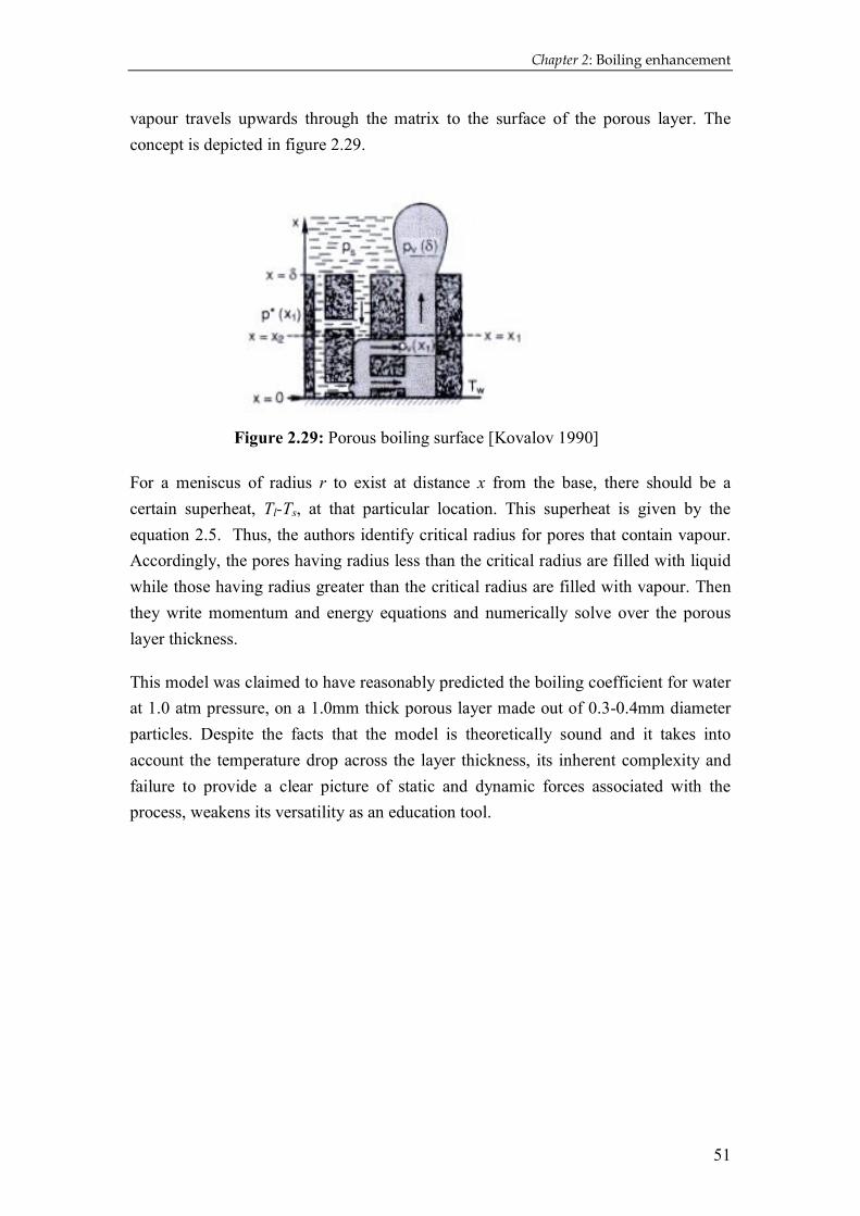
Chapter 2: Boiling enhancement
51
vapour travels upwards through the matrix to the surface of the porous layer. The
concept is depicted in figure 2.29.
Figure 2.29: Porous boiling surface [Kovalov 1990]
For a meniscus of radius r to exist at distance x from the base, there should be a
certain superheat, Tl-Ts, at that particular location. This superheat is given by the
equation 2.5. Thus, the authors identify critical radius for pores that contain vapour.
Accordingly, the pores having radius less than the critical radius are filled with liquid
while those having radius greater than the critical radius are filled with vapour. Then
they write momentum and energy equations and numerically solve over the porous
layer thickness.
This model was claimed to have reasonably predicted the boiling coefficient for water
at 1.0 atm pressure, on a 1.0mm thick porous layer made out of 0.3-0.4mm diameter
particles. Despite the facts that the model is theoretically sound and it takes into
account the temperature drop across the layer thickness, its inherent complexity and
failure to provide a clear picture of static and dynamic forces associated with the
process, weakens its versatility as an education tool.

Sanjeeva Witharana: Boiling of refrigerants on Enhanced surfaces
52
Figure 2.30: Predicted and experimental data on top, and test surfaces
in the bottom. [Nishikawa et al. 1983]
Nishikawa et al. [1983] developed an empirical correlation for boiling on porous
layers based on their test data from boiling R-11, R-113 and benzene at 1atm pressure.
The correlation is
( )
67.1708.0593.056.00284.0
22
2
001.0
=
∆
−
v
l
l
m
v
p
pm k
kdq
dqTk
q
ρρ
ελµδ
δλσδ &
&
& 2.40
Figure 2.30 illustrates the test surface parameters and a plot comparing the test data
and that predicted by the correlation.

Chapter 2: Boiling enhancement
53
Webb [1983] used seven sets of readily published experimental data to analyse the
degree of accuracy of Nishikawa et al. [1983] correlation. This data had been reported
from boiling R-11 and R-113 on porous coatings consisted of particles sized dp up to
1mm. At the wall heat flux value of 20 kW/m2, the correlation yielded ‘reasonably
good’ predictions for the ∆T.
Cieslinski et al. [2000] produced Aluminium coating by ‘modified’ gas-flame method
on 39 mm diameter circular Copper plates and conducted pool-boiling tests with
water. They used the experimental data to verify well-known correlations and
produced the plot presented in figure 2.31.
Figure 2.31: Predicted and experimental results. x-Nishikawa (1983), ∗-Mankovsliy, +- Smirnow, ◊-Tehver and -Ayub predictions. °- the experimental data [Cieslinski 2000].
Liter and Kaviany [2001] suggests theories to improve the critical heat flux (CHF)
by modulated (periodically non-uniform thickness) porous-layer coating. The theory
is a modified version of Zuber [1959] hydrodynamic theory, and based on the
hypothesis that the enhancement of the surface could be further improved by
separating liquid and vapour flow paths within the matrix. In a non-modulated
coating, liquid-vapour counter flow resists each other’s movement hindering the heat
transport from the surface to the liquid pool. The model is proposed for conical stacks
made of uniform diameter particles, as illustrated in figure 2.32(a), which are assumed
to be of uniform porosity.

Sanjeeva Witharana: Boiling of refrigerants on Enhanced surfaces
54
The model further assumes that, the local averaging of temperature and velocities are
valid and also, that there is a complete phase separation within the coating matrix. The
vapour escapes from between the stacks where the particle stacks and the base layer
(the bottom most particle layer) are liquid saturated. The liquid along the outer edge
of the stacks undergoes thin-film evaporation. The liquid in the stack core and in the
base layer is assumed to be stagnant.
CHF predicted by the present theory is expressed in the form,
( ) 21
, /..8
mvlathCHF qq λσρπ&& = 2.41
Where λm is a length scale characterizing the vapour escape location into the liquid
pool from the porous-layer coating. It is a function of geometrically determined
vapour escape paths and therefore a function of the porous structure. By reducing λm,
it should be possible to increase the CHF. Figure 2.32(b) shows the model predictions
and the experimental results obtained from boiling pentane on a copper particle-
sintered horizontal copper plate.
Figure 2.32(a): Schematic of the physical model [Liter and Kaviany 2001]

Chapter 2: Boiling enhancement
55
Figure 2.32(b): Predicted and experimentally obtained results
[Liter and Kaviany 2001]
For the plain surface, predicted qCHF =247 kW/m2 whereas the measure value was 245
kW/m2. For a coating of ε=0.4 and d=200µm, the predicted and measured values
were 478 kW/m2 and 480 kW/m2 respectively. For the modulated coatings; in the case
of predicted qCHF =762 kW/m2, the above stated equation predicted λm=1.46mm while
the designed value 8d was 1.6mm; in the case of predicted qCHF =712 kW/m2, the
designed value was 1.68mm, fairly higher than the designed value, which was 1mm.
2.8 Boiling enhancement – Goal of the present investigation
The foregoing discussion was devoted to review the history of the art of enhanced
surfaces from its inception to the present day. One aim of that effort was to increase
the knowledge of the historical development of the subject while pinpointing the
turning points and invaluable concepts and theories that contributed to the
development of the same art. Jacob [1931]’s observations on a roughened surface,
Griffith and Wallis [1960]’s theory of re-entrant cavities and related explanations,
Milton [1968]’s High Flux surface, Nakayama et al. [1980a,b, 1982]’s and O’Neil et
al. [1972]’s models, should be mentioned as breakthroughs in this specialised area.
Their observations, concepts and findings on boiling enhancement largely contributed
to the advancement of this science, paving the way for where it is today. From time to
time, J.R.Thome, A.E.Bergles, R.L.Webb and alike have presented comprehensive
literature collections to the scientific community.

Sanjeeva Witharana: Boiling of refrigerants on Enhanced surfaces
56
The concept of boiling on structured surfaces has been better understood and is
modelled fairly well in comparison to coated surfaces. The degree of enhancement
that a coated surface show was higher than that of many commercially popular
structured surfaces under similar test conditions according to Yilmaz and Westwater
[1981]. However, after an extensive literature survey, the author found a void for a
correlation that would model the parameters of a coated surface, viz., porosity,
thickness, particle size and cavity shape to predict its heat transfer performance.
The present investigation is intended to consist of two parts; an experimental part to
manufacture and test the optimised surface, and a modelling part to correlate the
performance to the surface parameters. In the fabrication stage, the readily available
information on well-established cavity geometries obtained on structured surfaces will
be used as a guide while, the coating thickness and porosity will be chosen based on
already published data on coated surfaces.

Chapter 3
THE EXPERIMENTAL SET UP AND PROCEDURE
The discussion thus far had been devoted to educate the reader about the principles of
boiling and the importance of boiling enhancement. An overview of the large amount
of literature published under these topics was also presented. At the end of chapter 2,
it was mentioned the need for a correlation that could explain the boiling mechanism
on enhanced planer surfaces. That will also identify the relationship between the
surface performance and the surface parameters. To develop such a universal
correlation, a substantial amount of data is required. These data should include boiling
performance on enhanced matrices, within a range of pressures and oil concentrations.
The surface parameters should also be varied from one surface to another. Thus, the
need arises for a versatile surface fabrication method, which is reliable and repeatable.
Presented in this chapter is the invention of a reliable and repeatable surface
fabrication technique in which the surface parameters too can be manipulated to a
great extent.
New terms, which will be introduced in the forthcoming text, are:
Test surface: the structure that is going to be tested for pool boiling of R-134a.
Test sample: the metal surface on which the surface has been produced
Sample holder/Prototype: the unit combination of the heater and the insulation, on
which the sample is mounted (or produced)
3.1 The sample holder
The surfaces were produced on one end of a circular solid copper bar of 25mm
diameter. Initially, a 100mm long piece was separated from a long copper bar, using a
lathe machine. This copper rod was going to serve dual purposes. One end of this cut-
piece was going to be used as the test surface. The other end will be used for the heat
supply. Since this is going to be used for pool boiling tests, there should be a sound

Sanjeeva Witharana: Boiling of refrigerants on Enhanced surfaces
58
insulation to minimise the heat leakage to the surrounding refrigerant. The insulation
material, in addition to its low thermal conductivity, should be chemically inert with
the refrigerant, easy to be machined to achieve the desired shape, be able to withstand
high temperatures (from the heater) and be cost-competitive. It was found that Teflon
met most of these criteria. Subsequently, Teflon was chosen as the insulating material
and a two-piece insulation block was manufactured.
The copper rod and the Teflon insulation together form the sample holder. The
illustration in figure 3.1 is a detailed drawing of the sample holder.
25
2060120
50
2
10
5
test surface
thermocoupleinserts
Copper rod
heater wire
Tefloninsulation
Figure 3.1: Detailed illustration of the sample holder
In the top half of the copper rod and also in the Teflon block, five holes were drilled
for the thermocouple inserts. In the bottom part of the copper rod, up to 40mm from
the bottom end, a spiral groove was machined to wind the heating wire. The two ends
of the heating wire come out through the bottom holes in the Teflon block, and are
connected to the power supply. Thus, the heat is transported through the copper rod
from the bottom end to the top end, where it would be dissipated to the surrounding
refrigerant.
The circular-shape Teflon block was manufactured in two separate parts. To the upper
part, the copper rod was press-fitted as shown in figure 3.2. To fasten the top and
bottom parts of the Teflon block, nuts and bolts were used. To prevent a possible
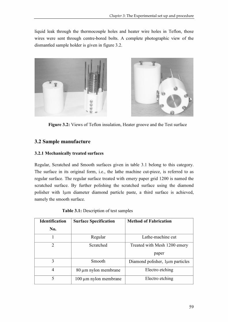
Chapter 3: The Experimental set up and procedure
59
liquid leak through the thermocouple holes and heater wire holes in Teflon, those
wires were sent through centre-bored bolts. A complete photographic view of the
dismantled sample holder is given in figure 3.2.
Figure 3.2: Views of Teflon insulation, Heater groove and the Test surface
3.2 Sample manufacture
3.2.1 Mechanically treated surfaces
Regular, Scratched and Smooth surfaces given in table 3.1 belong to this category.
The surface in its original form, i.e., the lathe machine cut-piece, is referred to as
regular surface. The regular surface treated with emery paper grid 1200 is named the
scratched surface. By further polishing the scratched surface using the diamond
polisher with 1µm diameter diamond particle paste, a third surface is achieved,
namely the smooth surface.
Table 3.1: Description of test samples
Identification
No.
Surface Specification Method of Fabrication
1 Regular Lathe-machine cut
2 Scratched Treated with Mesh 1200 emery
paper
3 Smooth Diamond polisher, 1µm particles
4 80 µm nylon membrane Electro etching
5 100 µm nylon membrane Electro etching

Sanjeeva Witharana: Boiling of refrigerants on Enhanced surfaces
60
3.2.2 Electro-chemically etched surfaces
The novel surfaces which going to be introduced in this work are known as electro-
chemically etched surfaces. The surface no. 4 and 5 given in table 3.1 falls into this
category. In the forthcoming discussion, the manufacturing procedure and the related
science will be explained.
The term ‘electro-chemical etching’ is fairly self-descriptive of the process involved
in it. It is a generally know fact that if a piece of metal is immersed in a strong acidic
solution, the metal piece will gradually dissolve into the acidic solution. This process
could be identified as etching. The amount of metal that is being removed from the
surface depends on the strength of the solution and the time duration. A greater
control over the amount of metal decay is possible by passing an electric current
through the solution, keeping the etching metal at the anode. Such a process is called
electro-chemical etching. Once the electric current, the strength of the acid solution
and the etching time is known, the mass decay could be calculated very accurately.
This calculation will further be explained in section 3.6.
For the present work, the electro-chemical etching technique was used to produce a
regular structure on the top end of the copper rod (shown in figure 3.1). Any extra
exposure would also be etched by the solution making errors in the calculation. To
prevent it, the copper rod was etched with the Teflon insulation on it. Figure 3.3
illustrates the electro-chemical etching set-up used in the present work. The sample
holder (prototype) was kept at anode (+) while the cathode (-) was another piece of
copper.
Anode(sample holder)
Cathode
Electrolyte
Figure 3.3: Schematic of the prototype etching

Chapter 3: The Experimental set up and procedure
61
At the Anode, the Cu surface decays by releasing Cu2+ ions to the acid solution. These
ions, then travel through the acid solution to the Cathode and deposit on it.
Subsequent Electro-etching chemical reactions are as follows:
At anode: Cu (s) Cu2+
(aq) + 2e- At cathode: Cu2+
(aq) + 2e- Cu (s)
3.3 Surface Preparation by electro-chemical Etching
In order to obtain a surface with a regular structure by this method, it is necessary to
have a pattern drawn on the surface. Otherwise, the whole surface will dissolve,
without a particular structure being formed on it. The patterning was an art rather than
a science. It is a key part of the present work. Patterning was followed by the
microscopic observation, followed by the electro-chemical etching. The
instrumentation and the sequential method are as follows.
3.3.1 Instruments
• The candidate surface
The candidate is the surface that is to be etched. At the initial stages, the
etching was experimented with sample copper strips of 0.5mm thickness and
25mm diameter. These etching experiments included different acid solutions,
solutions with different concentrations, different current densities and varying
time durations. The practice obtained through those initial experiments was
essentially helpful in etching the prototype (figure 3.3) very accurately.
The surface roughness directly influences the quality of etching. Scratches or
defects in the surface would make those particular areas to etch more than the
rest of the surface. For the best etching, the candidate surfaces were kept as
smooth as possible.
• Nylon net filters
Obtaining pores of desired size and shape on the copper surface was the prime
objective at this stage. Nylon net filters delivered by MilliporeTM, shown in
figure 3.4, could meet these demands. They were commercially available in
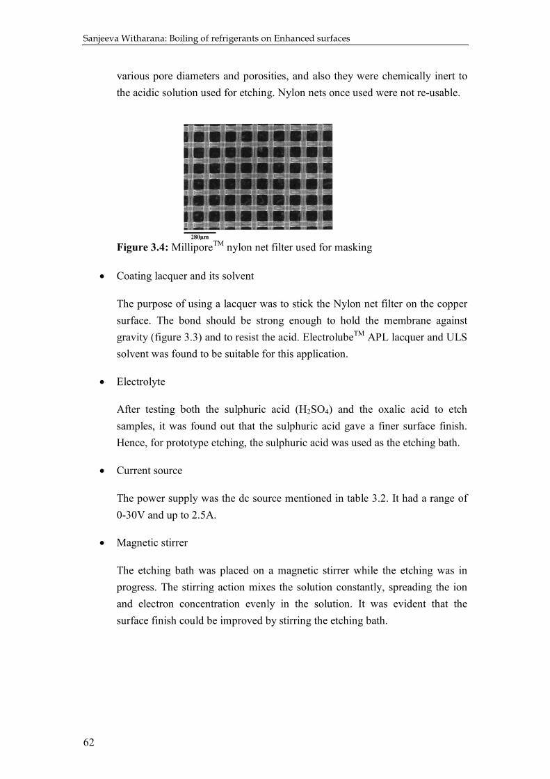
Sanjeeva Witharana: Boiling of refrigerants on Enhanced surfaces
62
various pore diameters and porosities, and also they were chemically inert to
the acidic solution used for etching. Nylon nets once used were not re-usable.
Figure 3.4: MilliporeTM nylon net filter used for masking
• Coating lacquer and its solvent
The purpose of using a lacquer was to stick the Nylon net filter on the copper
surface. The bond should be strong enough to hold the membrane against
gravity (figure 3.3) and to resist the acid. ElectrolubeTM APL lacquer and ULS
solvent was found to be suitable for this application.
• Electrolyte
After testing both the sulphuric acid (H2SO4) and the oxalic acid to etch
samples, it was found out that the sulphuric acid gave a finer surface finish.
Hence, for prototype etching, the sulphuric acid was used as the etching bath.
• Current source
The power supply was the dc source mentioned in table 3.2. It had a range of
0-30V and up to 2.5A.
• Magnetic stirrer
The etching bath was placed on a magnetic stirrer while the etching was in
progress. The stirring action mixes the solution constantly, spreading the ion
and electron concentration evenly in the solution. It was evident that the
surface finish could be improved by stirring the etching bath.

Chapter 3: The Experimental set up and procedure
63
3.3.2 Procedure
• Polish the surface
The polishing was done by using the Diamond polisher with 1µm diameter
particles.
• Clean the sample with Acetone
The sample surfaces were cleaned using the organic solvent ‘acetone’ to
remove dirt and other contaminants on it.
• Spray the coating on to the nylon net
The nylon net was kept in horizontal position and the coating lacquer was
sprayed on to it.
• Attach the nylon net on the sample (‘masking’ operation)
Soon after spraying was done, the net was placed on the sample surface. They
stick to each other very quickly.
• Observe through the microscope
Before the sample being sent for etching, the success of the masking operation
was verified by observing it through microscope (LOM). In case of the
masking was not satisfactory, either the sample had to be thrown away or to be
washed and reused from the beginning. Shown in figure 3.5 is a sample that
successfully went through masking.
• Etching
After the masking was verified for perfection, it was taken to the etching bath.
The sample/the prototype was fixed in the order shown in figure 3.3, with its
etching surface downwards facing the opposite electrode. Then, the power
supply was set to the desired voltage and the etching was started. The etching
bath was stirred by using a magnetic stirrer while etching the sample. The
starting time was recorded. After the pre-determined etching time had elapsed,
the power supply was shut down and sample was taken out of the etching bath.
The sample was quickly washed with water and acetone respectively, and
then, it was dried with compressed air.

Sanjeeva Witharana: Boiling of refrigerants on Enhanced surfaces
64
• Microscopic observation
The final product was now ready. The observations were made through the
LOM to verify the accuracy of dimensions. The image shown in figure 3.6 is
of an etched sample. It is now ready to test for boiling performance.
Figure 3.5: LOM image of a masked sample (x100)
Figure 3.6: LOM image of an electro- etched sample (x100)
3.4 Surface Preparation by electro-deposition
The instruments and the procedure described under sections 3.3.1 and 3.3.2 may also
be employed to produce a pore structure on a metal surface by electro-deposition. The
notable difference would be the electrolyte, which would be a copper salt like CuSO4
solution, and the anodic and cathodic reactions. The difference in the final surface
made of electro-deposition over that of electro-etched surface is that, in the former,
the particles will gather to the open area of the membrane whereas in the latter, the
particles are removed from the open area. And when the membrane is removed, the
surface in a 3-D view would look like a network of inter-connected channels in-
between the newly formed fins. Shown in the following two figures are the
microscopic images of electro-deposited regular pore structures produced by this

Chapter 3: The Experimental set up and procedure
65
author. The structure shown in figure 3.7(a) was obtained by electro-deposition on a
180µm nylon net, while the structure in figure 3.7(b) was from a 100µm nylon net.
Figure 3.7(a): LOM image of an electro- deposited surface, with the mask on (x100)
Figure 3.7(b): SEM micrograph of an electro deposited surface (x100)
An irregular porous structure too is obtainable on a copper surface by electro-
deposition. By omitting the masking operation, thus exposing the entire surface to the
electro-deposition bath, an irregular structure was obtained as shown in the LOM
image in figure 3.7(c). Such a structure was easier to obtain but difficult to re-
produce.
Figure 3.7(c): Irregular electro- deposition without using a mask.

Sanjeeva Witharana: Boiling of refrigerants on Enhanced surfaces
66
Electro-deposition too is a delicate art in the same way as electro-etching. It consumes
a considerable time and effort to master the art of electro-deposition. Due to the time
constraints, the work of this thesis was more concentrated to etched surfaces, leaving
behind deposited surfaces for future work.
3.5 Boiling, regulation and data collection
3.5.1 Boiling
Figure 3.8 shows the pool boiling test rig. This test rig was used to boil the
refrigerant at a desired pressure level. Tank B is the boiling chamber. Tank A is the
condensing chamber. Vapour formed by the boiling refrigerant escapes through the
tube V, to the chamber A. In A, this vapour condenses and flows back to B through the
tube L. The vapour flow from B to A is driven by the slight pressure difference caused
by the vapour generation in B and vapour condensation in A. The liquid flow from A
to B occurs due to gravity. Condensation in tank A is realised by aid of a coil, which is
the evaporator of a refrigerating machine. This secondary system is also shown in
figure 3.8.
When the tank B needed to be evacuated, the refrigerant was pumped into tank A. In
such occasions, the liquid was evacuated first, and then the vapour. Liquid evacuation
was possible by closing the valve in the vapour line while running the compressor.
Through the sight-glass it could be seen if the tank B was empty of liquid. To
evacuate the vapour, the liquid valve was closed and the vapour valve was opened.
After running the compressor for about half an hour, the pressure in B could be
brought down to 2 bar, which was the minimum possible level. The still remaining
vapour had to be released to the atmosphere.
In order to start the boiling tests, the chamber B had to be opened and the sample
holder had to be firmly placed in it. Before replacing the lid, the thermocouple
contacts with the rod were verified by using a multimeter. Then the boiling chamber
was closed. The temperature and heater wires were connected to the instruments as
shown in the same figure. If the thermocouples were connected properly, the logger
now started to display the temperature readings.
Before filling the chamber with the refrigerant, it was evacuated by using a vacuum
pump. The pressure of the chamber was read on the logger display. If there were no
leaks, the evacuation process normally took less than one hour. Once the evacuation

Chapter 3: The Experimental set up and procedure
67
process was completed, the chamber B was filled by refrigerant from chamber A, first
by gradually opening the liquid valve and then by opening the vapour valve.
The amount of refrigerant was chosen so as to maintain a fixed level in all
experiments. The test pressure was set in the logger. Then, the refrigeration system
was started. The system was let alone to run for six hours before any experiments
were conducted. During this time, it was expected to reach the thermal equilibrium
with the surroundings. When the system was ready, the tests were started by giving a
heat input to the sample holder. The magnitude of the heat input was known from the
electric current and the voltage, indicated on the d/c power supply.
data collection& storage
multimeter
P
H
T
loggerpowersource
condenser
V
L
M N
A
B
TEV
E
P - PressureT - TemperatureH - Heat supply
L - Liquid line
A,B - Pressure vessels
V - Vapour lineM - Magnetic ValveN - Needle ValveE - Emptying Valve
RegulationMeasurementData
Figure 3.8: Test Rig with the sample inside boiling chamber B

Sanjeeva Witharana: Boiling of refrigerants on Enhanced surfaces
68
3.5.2 Regulation and Data collection
The set pressure is maintained constant throughout an experiment by the combination
of the logger, the pressure transducer P and the magnetic valve M. The logger senses
the pressure level in the boiling chamber through P and compares it with the set value
fed to it by the researcher. To go from a higher pressure level to a lower pressure
level, the logger sends a signal to M to open the suction line of the refrigerating
machine, which otherwise is at closed position.
The hand operated needle valve N, functions as a means of fine adjustment, when the
regulation system is trying to reach the set pressure level by opening and closing the
magnetic valve, M.
As well as pressure, the logger also reads the spontaneous temperatures. In total it
reads six temperatures, of the five thermocouples in the sample holder (figure 3.1),
and of the one in the liquid. The digital multimeter Fluke 45 displays the electric
current passing through and the voltage across the heater wire. Real-time values of
pressure, temperature, electric current and the voltage are then transferred to HP VEE
software in the PC, which was programmed to present a graphical display on the
monitor. When the temperature lines on the monitor was appeared stable, the data
collection was started by activating the MS Excel work sheet. The real-time data was
collected and registered in ever fifth second till twenty data points were collected.
Table 3.2 presents a list of instruments and devices used to perform measurements,
data collection and surface observation.
Table 3.2: Measuring instruments and devices
Instrument/ Device
Manufacturer Type Error Limits (As specified by the manufacturer)
Thermocouples Pentronic T ± 0.5 °C Pressure transducer
Druck Ltd. PDCR911 ± 0.1% BSL
D/C Power source
Velleman PS613 0.05V, 0.005A
Multimeter Fluke 45 0.5*10-3V, 0.5*10-4A PC program Hewlett Packard HP VEE Ver 5.0
(1998)
Data Storage Microsoft MS Excel Light optical microscope
Olympus PMG3

Chapter 3: The Experimental set up and procedure
69
3.6 Calculations
3.6.1 Pore depth
For a given electric current I supplied over a time t, the pore depth h can be
determined using the following equations.
The Cu Anode (the sample) dissolves in Sulphuric Acid:
Cu (s) Cu2+(aq) + 2e- 3.1
The number of e- moles dissolved in to the solution n:
F
tIn
..= 3.2
Where F is the Faraday constant. The mass of Cu transported into the solution m:
2
.nMm Cu= 3.3
Finally, the pore depth h is given by:
ερ ..A
mh = 3.4
Where, ρ is the density of copper, and, A and ε are the base area and the porosity of
the surface respectively.
For a sample calculation, consider the surface number 5 in table 3.1. The nylon
membrane chosen was NY100, where the specified pore diameter and porosity were
100µm and 44% respectively. The electrolyte was 1M Sulphuric acid (H2SO4), the
current was 0.05A and the etching time was 3 hours. By following the equations 3.1
through 3.4, the depth of the pores was calculated to 92µm. This was how in reality
the depths of the surfaces number 4 and 5 were calculated in table 4.1, in the next
chapter.
3.6.2 Heat loss through the insulation
Figure 3.1 illustrated the heater arrangement with the Teflon insulation. When the
heat is supplied to the copper rod, there will be a certain heat leakage through the
insulation to the surrounding refrigerant. The amount of heat leakage is possible to be
estimated using the Fourier’s law of heat conduction.

Sanjeeva Witharana: Boiling of refrigerants on Enhanced surfaces
70
Ts,1 Ts,2 Tx Tw Qr Qr Qr Qr Qa Qb (a) (b) Figure 3.9: (a) Heat leakage through insulation (b) Heat transport in the rod
Shown in figure 3.9(a) is a schematic of the heat flow through the insulation. The
temperature of the inner wall Ts,1 is larger than the outer wall temperature Ts,2, thus,
the heat flows of Qr and Qb occurs across the radial and bottom walls respectively.
Total heat supplied to the rod Q can be expressed as, Q = Qa+Qb+Qr, where Qa is the
heat flow in the axial direction as shown in figure 3.9(b).
Assuming one-dimensional heat flow, the radial heat loss Qr can be calculated by following Fourier’s law of heat conduction [Incropera and DeWitt 1996],
( )
−=
1
2
2,1,
ln
2
r
r
TTLkQ
ss
r
π 3.5
Where L and r1 are the height and the radius of the copper rod, while, k and r2 are the
thermal conductivity and the outer radius of the insulation. The unknowns in this
equation would be Ts,1 and Ts,2. The centreline temperatures of the copper rod are
known by measurements. Hence, a value for Ts,1 may be obtained under the
assumption that the copper rod is uniformly heated in the radial direction. The
remaining unknown of Ts,2 may be approximated to the temperature of the
surrounding liquid. Also, Qb would be calculated by writing the Fourier’s law for
conduction through a plane wall, given by equation 3.6 below.
For a sample calculation, consider a case where R-134a is boiled under a pressure of
5bar at a heat input of 30W. The relevant temperatures are shown in the figure 3.14 at
the end of this chapter. The value for the inner wall temperature of the Teflon block
Ts,1, in equation 3.5, and also in equation 3.6, will be reasonably assumed as the
temperature reading of the bottom-most thermocouple. Therefore, Ts,1=25.8°C, while
Ts,2=15.3°C. The thermal conductivity k for teflon is 0.35 W/mK. The geometrical
dimensions are as per the figure 3.1. Finally, the calculation returns Qr=3.33W and
Qb=0.009W. This means that the total heat loss Qb+Qr is around 11% of the total heat

Chapter 3: The Experimental set up and procedure
71
supplied to the rod Q. This heat loss will be neglected in the heat transfer calculations
in chapter 4, approximating Qa to Q.
3.6.3 Surface temperature
It was earlier stated that the surface modifications were done on one end of the copper
rod. Therefore, by measuring the temperatures of few known points in the rod, it
should be possible to know the surface temperature by extrapolation. Consider figure
3.9 (b).
Writing the Fourier’s law of heat conduction for the axial heat flow Qa,
X
TkAQa ∂
∂= 3.6
Where, A is the cross section area of the rod.
Thus, the temperature gradient in the copper rod would be:
kA
Q
X
T a=∂∂
3.7
The quantity Qa was approximated to Q after neglecting the losses as described in the
foregoing paragraph. Hence, Qa becomes a known quantity, which is the heat input to
the rod through the heater wires. Temperature of a single point in the rod at a known
distance from the surface Tx, would then be sufficient to calculate the temperature
gradient in the rod, and hence, to extrapolate the surface temperature Tw. However at
this point, it should be noted that the temperature measurements at five points along
the rod were taken for the sake of verifying the accuracy of the thermocouple
readings. This part would be further treated under section 3.7.3.
3.6.4 Heat transfer coefficient
Newton’s law of cooling is applicable to calculate the heat transfer coefficient
between the surface and the liquid.
( )lw TTAhQ −= .. 3.8
The heat input Q, base area of the surface A, wall temperature Tw and the liquid
temperature Tl, are all known by now. Hence, the heat transfer coefficient h could be
determined.
Cooper [1984] correlation also provides an estimate for the boiling heat transfer
coefficient on conventional surfaces.

Sanjeeva Witharana: Boiling of refrigerants on Enhanced surfaces
72
( ) ( ) 67.05.055.0
10log2.012.0 ...log...55 .10 qMPPCh fr
Rr
P &−−− −= 3.9
Where Mf is the molar mass of the refrigerant, and the roughness parameter PR is
suggested to be equal to 1 for optically smooth surfaces. Also, the constant C set to be
equal to 1 for horizontal plane surfaces and 1.7 for horizontal copper cylinders.
3.7 Problems from design to operation
It was stated that figure 3.1 was the final form of the heater arrangement. Getting to
there was a deterministic and time-consuming exercise, passing a number of stages
and facing many obstacles. Those encounters are treated in this section.
3.7.1 Choice of a Heater
The size and the shape of the heater should match the dimensions of the copper rod.
That means, the heater should be 25mm in diameter and of cylindrical shape. At the
same time, the heater has to be able to supply and withstand the desired maximum
power duty to create a heat flux of 100 kW/m2 on the surface. The commercially
available heaters, such as OMEGA and MINCO, could not deliver such high heat
fluxes. Consequently it was decided to design a heater by winding a high-resistance
wire around the copper rod. The resistance of the wire was 14.8 Ω/m.
3.7.2 The Bonding mechanism for the Sample and the Heater
In this project, initially, the intention was to manufacture the test surface (similar to
that shown in fig 3.5) and the heater arrangement (similar to that shown in fig 3.1) in
two separate pieces. Then, to attach these two pieces to each other, some kind of a
bonding mechanism was supposed to be found. Also, the two pieces should be able to
be detached from each other when needed, and also the bonding agent should be able
to be completely removed from the surfaces. By this way, one heater arrangement
would suffice to conduct a whole series of tests, merely by changing the test surfaces.
Shown in figure 3.10 is a schematic of the first form of the heater arrangement that
was produced. In this scheme, Teflon insulation was manufactured as one piece in
contrast to the one lately produced, which was shown in figure 3.1. Another notable
difference is that, in here two thermocouples are provided on top of the copper
surface. The test surface, which is manufactured separately on a thin copper plate of
0.5mm thickness, was attached to the ‘top surface’ in the way illustrated in figure
3.11. Then, a suitable bonding agent was needed to be found.

Chapter 3: The Experimental set up and procedure
73
The major concerns in choosing the bonding agent were its ability to spread evenly on
the surface covering the whole of it, and to maintain a uniform thickness all over. By
meeting these two parameters, a uniform heat flow was expected, from the top surface
to the test sample. Thus, when it comes to heat transfer calculations, it was reasonable
to assume a constant resistance to heat flow, throughout the surface area. Large
collections of bonding agents were always available. Few of them were selected and
experimented for their suitability. They included, the ‘woods metal’ (a frequently
used solder in the laboratory), RA Solder Cream (from Multicore Solders Limited)
and a copper tape.
8thermocouple
inserts
Copper rod
Tefloninsulation
heater wireinsert
top surface
2
Figure 3.10: The heater arrangement in its initial form
(The unspecified dimensions are as shown in fig 3.1)
copper teflon
thermocoupletest surface
bondingagent
top surface
Figure 3.11: A vertical cross-section of the sample-heater attachment

Sanjeeva Witharana: Boiling of refrigerants on Enhanced surfaces
74
(a) Wood’s metal
This metal has been used in the laboratory for soldering purposes, for a fairly
long time. Wood’s metal is a lead-alloy that possesses a thermal conductivity
of about 40 W/mK, low meting point (around 90°C) and fast spreading.
However in this application, the Wood’s metal failed to show the desired
quality of uniform solder thickness.
(b) RA Solder Cream
A solder paste curing at 180°C, the RA Solder Cream was expected to provide
the uniform solder thickness. It had a thermal conductivity of 15 W/mK and
was easily applicable on metal surfaces. Subsequently, a layer of RA Solder
Cream was applied on the bottom of the test sample, it was placed on the top
surface, a pressure was applied with a clamp and the joint was placed in a
furnace at 180°C to cure. After passing the specified curing time in the
furnace, the set-up was allowed to cool down in the atmosphere. Every time a
sample was changed, the set- had to undergo a heating-cooling cycle. This
bonding technique worked perfectly well for first two heating-cooling cycles.
The thermal expansion coefficients of copper and Teflon are different. When
the Teflon-copper press-fit could not withstand the temperature cycles any
longer, the press-fit got loosened, providing enough room for the refrigerant
liquid to leak through. Liquid leakage cools the copper rod from inside.
Hence, the temperature readings would not provide the true picture.
(c) The copper tape
The double-sticking copper tape became another option to attach the sample to
the top surface. These tapes are commercially available and easy to use. The
tape used in this work was a 3M electric tapeTM, the nominal total thickness
and the resistance of which were 0.081mm and 0.005Ω respectively [ELFA
catalogue 1996]. Unfortunately, the copper tape failed to maintain its grip in
the R-134a liquid. Therefore, it did not qualify as a reliable bonding agent.

Chapter 3: The Experimental set up and procedure
75
The uppermost thermocouples shown in figure 3.11, due to their location, would exert
an upward thrust on the sample. This thrust, though small in magnitude, would be
enough to lift the sample upwards, thus breaking the bond. Moreover, loose
thermocouples will report wrong temperatures. To solve this problem, the scheme
illustrated in figure 3.12 was produced and experimented. In this scheme, the top
surface did not hold any thermocouples. Two top thermocouples were instead located
inside the copper rod, very close to the top surface.
The modified sample-heater attachment maintained the thermocouples stable in
position and reliable in readings. However, this scheme too could not answer the
issues raised in (a), (b) and (c).
copper teflon
thermocouple
test sample
bondingagent
Figure 3.12: A vertical cross-section of the modified sample-heater
attachment
3.7.3 Temperature measurements
Undoubtedly, the temperature values are the most precious data in this research
project. According to equation 3.8, a 1°C measurement error in the temperature
difference (Tw-Tl) could lead to up to 20% error in the heat transfer coefficient h.
Therefore, every effort was devoted to assure the accuracy of the temperature
measurements. In addition to the thermocouple accuracy, the reliability and stability
of the temperature measuring points were also to be addressed.
The accuracy of the thermocouples was confirmed by an ice-bath test. Having done
that, it would be fair to expect that they would give accurate temperature readings
while running the boiling tests. A method of verification also exists. For a given heat
input to the copper rod, the temperature drop between two measuring points could be
calculated by a heat conduction calculation using the equation 3.7, with a provision
for heat leakage through the Teflon. However, the accuracy in the measurement of
temperature difference is estimated to ±0.1°C.

Sanjeeva Witharana: Boiling of refrigerants on Enhanced surfaces
76
One basic question faced in temperature measurement was related to the power
supply. When the power supply was an a/c power source, a change from one heat
input to another disturbed the temperature readings. This disturbance did not
disappear even after the heater stabilised in the new heat level. Hence, some
thermocouples continuously indicated a wrong temperature. The problem of
temperature disturbance completely disappeared as soon as the a/c source was
replaced by the d/c power source.
The liquid leaking between copper and Teflon walls was still the major problem. The
leakage could be physically witnessed by looking through the sight-glass in the
boiling chamber (figure 3.8). If bubbles are escaping through the thermocouple holes,
that would mean liquid leakage. Also by examining the temperature profiles of
thermocouples, the liquid leakage could be confirmed. Figure 3.13 shows the
reflection of liquid leakage on thermocouple readings. It is clear that the temperature
readings are highly deviated from a straight line, at each heat input.
Figure 3.13: Liquid leakage through the walls For a comparison, figure 3.14 presents the temperature readings in a non-leaking system. This non-leaking system was the one illustrated in figure 3.1.
0
5
10
15
20
25
30
35
0 5 10 15 20 25 30dist. from bottom-most thermocouple (mm)
tem
p. r
ea
din
g (
°C)
10W 20W 30W 40W 50W T-liq

Chapter 3: The Experimental set up and procedure
77
Figure 3.14: Straight temperature lines in a non-leaking system
0
5
10
15
20
25
30
35
0 5 10 15 20 25 30 35dist. from bottom-most thermocouple (mm)
tem
p. r
ead
ing
(°C
)
10W 20W 30W 40W 50W T-liq

Chapter 4
EXPERIMENTAL RESULTS
In the foregoing chapter, membrane-based etching and plating techniques were
introduced to achieve well-defined pore structures on plane copper surfaces. The
applicability of these production techniques was verified by producing few sample
surfaces consisting of pores of circular shape, known size and porosity. At the same
time, a leak-proof sample holder was designed and manufactured. The pool boiling
test-rig was explained in detail. Trial and error experience in attaching the samples to
the sample holder was also presented.
In the forthcoming discussion, the experimental results obtained from pool boiling
will be presented and discussed. The aim of these experiments was to investigate the
heat transfer coefficients in pool boiling of R-134a on horizontal flat surfaces with
different surface structures. Experiments were conducted at three pressure levels, 5
bar, 4 bar and 3 bar with oil concentrations 0%, 1% and 2% in the heat flux interval
20 kW/m2 to 100 kW/m2. During the discussion, at each stage, comparisons will be
done between the novel surfaces and the conventional surfaces.
4.1 Samples and test conditions
The method of fabrication for each sample was already mentioned in table 3.2. Given
in table 4.1 is a summary of tests. It should be noted that the surface numbers in table
3.2 and table 4.1 are essentially the same.

Sanjeeva Witharana: Boiling of refrigerants on Enhanced surfaces
80
Table 4.1: Description of test surfaces and test pressures (d, and h are the diameter
and depth of pores, and ε is the porosity of the surface)
No. Surface description 3 bar 4 bar 5 bar
1 Regular x x
2 Scratched x x x
3 Smooth x x x
4 Etched I: d=60 µm, h=240 µm, ε=40% x x x
5 Etched II: d=80 µm, h=92 µm, ε=44% x x x
4.1.1 Pore diameter, Pore depth and the Porosity
The manufacturer of the Nylon membranes specifies the pore diameter and the
porosity. Depending on the requirement and the availability of the product, the
appropriate membrane could be purchased. Shown in table 4.2 are the nylon
membranes used to manufacture the surfaces of interest.
Table 4.2: Product specification of MilliporeTM Nylon Membranes
Surface name Membrane Specifications
Pore diam. (µm) Porosity (%) Thickness (µm)
Etched I 80 40 75
Etched II 100 44 80
Once the right membrane is chose, for example with pore diameter of 100 µm, it is
customary to expect the membrane to produce 100 µm pores. However, a comparison
of table 4.1and table 4.2 shows that this was not the case. The pore diameters of
etched surfaces mentioned in table 4.1 is smaller than the diameters of respective
membranes used to produce those surfaces. The shrinkage in size may be explained in
terms of the capillary action of the coating lacquer. The coating lacquer, which is
sprayed onto the net as explained in section 3.3, spreads along the interior walls of
each pore. The result is the pore diameter after applying the lacquer is smaller than
the nominal pore diameter. This capillary action also makes the square-shape pores to

Chapter 4: Experimental results
81
circular shape. The shape difference is also noticed by comparing the figures 3.3.1
and 3.3.2. The pore depths were calculated in the fashion outlined in section 3.6.1 in
chapter 3.
4.2 Presentation and discussion of results
Shown below are the experimental results obtained from a series of pool boiling tests.
In each occasion, the heat flux q& was calculated as,
q& = AQ / , Where Q was the heat input from the heater neglecting losses (from
section 3.6.2) and A is the base area of the surface. According to this definition of the
base area, it remained unchanged irrespective of what the surface structure was.
Also, the heat transfer coefficient (HTC) was determined by,
( )lw TTAhQ −= .. , as explained under section 3.6.4, and with standard notations given
above.
And, the order of heating was first increasing, and then decreasing the surface heat
flux. However, the data presented on the diagrams are actually for the decreasing heat
flux. It is generally known that the decreasing heat flux data are more accurate due to
the facts that the boiling is more stable and the hysteresis effects are eliminated etc.
4.2.1 Wall superheat and heat transfer coefficient
Figure 4.1 illustrates the wall superheats (Tw-Tl) in boiling, in the heat flux ( q& )
interval of interest.

Sanjeeva Witharana: Boiling of refrigerants on Enhanced surfaces
82
Figure 4.1: R-134a boiling at 5bar. Wall superheat vs. Surface heat flux.
When the heat input was 20 kW/m2, the scratched surface has boiled the refrigerant
with the lowest wall superheat. That was approximately 25% lower than the Etched I
and about 30% than Etched II. This leading trend has continued throughout the heat
flux interval up to the highest heat level. However, the etched surfaces seen
approaching the performance of the scratched surface, as the heat flux is increasing.
As a result, it is observed that the initial gap of 25-30% in T∆ has narrowed to 5-
10% at the end. An extrapolation exercise would show that the three lines would soon
intersect at a heat flux little higher than the maximum shown in the plot.
Looking from the other end, the etched surface have shown up to 30% lower wall
superheat to that of the smooth surface and 25% to that of the regular surface. This in
fact is a positive development.
Turning to the boiling heat transfer coefficient (HTC) of each surface, figure 4.2
shows the values of HTC for boiling of R-134a at 5bar pressure. These results are
basically a reflection of the observations made in the former figure.
0
20
40
60
80
100
120
0 1 2 3 4 5 6 7 8 9Tw - Tl (K)
su
rfa
ce
he
at
flu
x (
kW
/m2 )
smoothregularEtched IEtched IIscratched

Chapter 4: Experimental results
83
0
4000
8000
12000
16000
20000
0 20 40 60 80 100 120surface heat flux (kW/m2)
HT
C (
W/m
2 K)
SmoothRegularEtched IEtched IIScratched
Figure 4.2: R-134a boiling at 5bar. Experimentally obtained HTC
At the upper limit of the heat flux, the novel surfaces are displaying far better heat
transfer rates from the surface to the liquid, as big as 30-50% to that of the smooth
surface. The advantage diminishes as the heat flux decreases, in spite of the scratched
surface holding the dominance.
Summarising the results for boiling at 5bar, the novel surfaces have indicated a very
close behaviour to each other, both showing approximately the same degree of
enhancement compared to a smooth surface.
Experimental results on boiling R-134a at 4bar pressure, plotted in figure 4.3, closely
follow the trend of boiling at 5bar. Notably, the data for regular surface was not
available for this case. Nevertheless, the superiority of scratched surface was still
dominating while the benefits of the novel surfaces gradually diminished towards the
lower limit of the surface heat flux.
The picture is slightly different when it comes to boiling of R-134a under a pressure
of 3bar. Referring to figure 4.4, it is possible to observe that the novel surfaces have
marginally surpassed the performance of a scratched surface at the upper heat flux
limit. This is a notable difference when compared to the cases of boiling at 4bar and
5bar pressures. In addition, the novel surfaces have maintained its superiority over the
smooth surface recording approximately 40% increase in HTC. However, these
observations itself do not provide enough evidence to make a distinction in

Sanjeeva Witharana: Boiling of refrigerants on Enhanced surfaces
84
performance between the two novel surfaces. Their performances were very much
alike under the present test conditions.
0
2000
4000
6000
8000
10000
12000
14000
16000
18000
0 20 40 60 80 100 120surface heat flux (kW/m2)
HT
C (
W/m
2 K)
SmoothEtched IEtched IIScratched
Figure 4.3: R-134a boiling at 4bar. Experimentally obtained HTC
0
2000
4000
6000
8000
10000
12000
14000
0 20 40 60 80 100 120surface heat flux (kW/m2)
HT
C (
W/m
2 K)
SmoothRegularEtched IEtched IIScratched
Figure 4.4: R-134a boiling at 3bar. Experimentally obtained HTC

Chapter 4: Experimental results
85
4.2.2 Evaluation of results
As an evaluation, the experimentally obtained heat transfer coefficients will be
compared with the values obtained from the Cooper [1984] correlation. This
correlation, also mentioned earlier as equation 3.9, was proposed for pool boiling of
liquids on horizontal plane surfaces and horizontal copper cylinders.
( ) ( ) 67.05.055.0
10log2.012.0 ...log...55 .10 qMPPCh fr
Rr
P &−−− −=
Cooper [1984] suggested the constant C be assigned a value of 1 for boiling on
horizontally oriented surfaces. He further suggested the surface roughness parameter
PR =1 for ‘optically smooth surfaces’.
In the present study, the Rp for three samples were measured using a Zygo New View
5010 (Zygo corporation, USA) profilometer. These measurements were performed at
the Institute of surface chemistry (YKI) of the KTH. Three measuring points were
taken on each sample. These points are numbered as P1, P2, and P3 and the
respective Rp values are given in table 4.3.
Table 4.3: Measured Rp values for test samples
Name of sample
Measuring point Measured Rp (µm)
Scratched P1 2.17
P2 1.69
P3 2.37
Regular P1 3.5
P2 3.34
P3 3.63
Etched-II P1 42.57
P2 37.33
P3 41.68
The first comparison between the experimentally obtained HTC and the Cooper
[1984] HTC will be made for boiling on smooth surfaces. The condition of optical
smoothness is assumed in this case, which assigns the value PR =1. Plotted in figure

Sanjeeva Witharana: Boiling of refrigerants on Enhanced surfaces
86
4.5 are the experimental and Cooper HTC for boiling of R-134a under 3bar, 4bar and
5bar pressure.
0
2000
4000
6000
8000
10000
12000
14000
0 20 40 60 80 100 120surface heat flux (kW/m2)
HT
C (
W/m
2 K)
3 bar_Exp 3 bar_Cooper4 bar_Exp 4 bar_Cooper5 bar_Exp 5 bar_Cooper
Figure 4.5: Smooth surface. Experimentally determined HTC vs. Cooper HTC
Now, by examining figure 4.5, one would recognise a considerably large difference
between the experimental values and the Cooper values. However, recalling the fact
that the Cooper’s constant C was kept at 1 for this exercise, it should be also possible
to make up for the gap by changing the value of the constant C. In fact, it is also
found that the ratio of HTCexp/HTCCooper is again dependent on the surface heat flux.
This is illustrated in table 4.3.

Chapter 4: Experimental results
87
Table 4.4: Suggested new constants for boiling on smooth plane surfaces
Saturation Value for Constant C
Pressure (bar) Heat flux 20 (kW/ m2)
Heat flux 100 (kW/ m2)
3 1.08 1.15
4 1.15 1.18
5 1.33 1.22
For each of the scratched, regular, and etched-II surfaces, the arithmetic mean of the
measured Rp values is used for HTC calculation using the Cooper correlation. These
mean values are given in table 4.5.
Table 4.5: Mean Rp values for test samples
Name of surface Mean Rp (µm)
Scratched 2.08
Regular 3.49
Etched-II 40.53
In the following diagrams, the comparison of HTC for scratched, regular, and etched-
II surfaces are illustrated. The experimentally calculated values for the regular
surface, shown in figure 4.7, reasonably agree with Cooper values, in a range of
±10%. However for scratched surface, the Cooper correlation has under-predicted the
experimental values as shown in figure 4.6. Evident from figure 4.8 is the fact that,
for the etched-II surface, which is having the highest Rp value, the Cooper correlation
has largely over-predicted the experimental values.
If these graphical observations are interpreted to the surface roughness values in table
4.5, there is a clearly visible trend. The trend is that, in the Rp value interval of 2.08 to
40.53, the prediction from the Cooper correlation crosses from under-prediction to
over- prediction. Interestingly, the trend of under-prediction is confirmed from figure
4.5, where it was assumed that PR =1.

Sanjeeva Witharana: Boiling of refrigerants on Enhanced surfaces
88
0
4000
8000
12000
16000
20000
0 20 40 60 80 100 120surface heat flux (kW/m2)
HT
C (
W/m
2K
)3bar-Exp 3 bar-Cooper4bar-Exp 4bar-Cooper5bar-Exp 5 bar-Cooper
Figure 4.6: Scratched surface. Experimentally determined HTC vs. Cooper HTC
0
2000
4000
6000
8000
10000
12000
14000
16000
0 20 40 60 80 100 120surface heat flux (kW/m2)
HT
C (
W/m
2K
)
3 bar-Exp 3 bar-Cooper5 bar-Exp 5 bar-Cooper
Figure 4.7: Regular surface. Experimentally determined HTC vs. Cooper HTC

Chapter 4: Experimental results
89
0
5000
10000
15000
20000
25000
0 20 40 60 80 100 120surface heat flux (kW/m2)
HT
C (
W/m
2K
)3 bar-Exp 3 bar-Cooper4 bar-Exp 4 bar-Cooper5 bar-Exp 5 bar-Cooper
Figure 4.8: Etched-II surface. Experimentally determined HTC vs. Cooper HTC
4.2.3 Oil tests
The results presented thus far were for the boiling of oil-free refrigerant R-134a. In
reality, in any refrigeration system, there is some oil volume present in the refrigerant.
This oil, which is the compressor lubricant, is mixed with the refrigerant and
circulates in the system. The objective of the following experiments was to
investigate the influence of oil concentration on the boiling heat transfer coefficient.
The oil used for these experiments was synthetic refrigeration oil named EAL Arctic
22CC produced by Mobil. To add the oil to the refrigerant, first the boiling chamber
(refer to figure 3.5 in chapter 3) was emptied of refrigerant, and then it was opened,
and the measured quantity of oil was poured into the chamber. The oil was
hydrophilic thus the exposure to the atmosphere would make it to absorb water. To
avoid it, the chamber was closed immediately after pouring the oil into it.
Consequently the chamber was vacuumed from the top of it, again to prevent the oil
escape through the vacuum pump. The task was completed by filling in the refrigerant
to the tank. The heat supply and the measurements were performed in a similar way
to those described before.

Sanjeeva Witharana: Boiling of refrigerants on Enhanced surfaces
90
Oil tests were conducted on Etched II surface under a pressure of 5 bar. In the first
series of tests, oil concentration was kept at 1 vol.%. In the second series, another 1
vol.% was added to the refrigerant, which made the total oil concentration to 2 vol.%.
Shown in figure 4.9 is the summery of the oil tests and the corresponding non-oil
tests. The values shown in the figure are based on decreasing heat flux.
0
4000
8000
12000
16000
20000
0 20 40 60 80 100 120surface heat flux (kW/m2)
HT
C (
W/m
2 K)
0% 1% 2%
Figure 4.9: Boiling of R-134a and oil mixture on Etched II surface, at 5bar pressure.
Referring to figure 4.9, it can be stated that the addition of oil to R-134a has, in
general, lead to the degradation of the boiling heat transfer coefficient. However,
there is one exception at 20 kW/m2 where the addition of 1 vol.% of oil has resulted a
15% increase in the HTC.
In the tests with oil, a slight deviation of the saturation temperature was observed.
This might have been caused by a minor contamination of the R-134a by some
means. However, since the heat transfer coefficients are calculated from measured
temperatures, this deviation is not believed to have caused a noticeable effect on the
displayed HTC.

Chapter 4: Experimental results
91
4.2.4 Boiling hysteresis
Boiling hysteresis had been observed on enhanced surfaces as mentioned in chapter 2.
It had been reported that the hysteresis effect was higher in coated surfaces compared
to structured surfaces. In an effort to study this phenomenon on present surfaces, the
boiling of R-134a on Etched II surface under a pressure of 5 bar was investigated.
The refrigerant was initially oil free, and then it was mixed with the ester oil
mentioned under section 4.2.3, at 1 vol.% and 2 vol.% concentrations respectively.
The experimental results are illustrated in figure 4.7.
The data for the non-oil refrigerant in figure 4.10 shows almost no signs of boiling
hysteresis for the surface Etched II. A trend line analysis of data corresponding to the
refrigerant with 2 vol.% of oil would show a hysteresis occurring around 9°C of wall
superheat. In addition, a very clear picture of hysteresis is witnessed with 1vol.% oil
in the refrigerant. In that case, one heating cycle, meaning the heating starting at the
bottom limit, increasing to the top limit and again decreasing to the initial level, the
surface has displayed approximately 7°C and 4°C of wall superheats at the two ends
respectively. Consequently, the T∆ due to the hysteresis calculates to nearly 3°C.
0
20
40
60
80
100
120
0 2 4 6 8 10 12Tw - Tl (K)
su
rfa
ce
he
at
flu
x (
kW
/m2 )
0% increasing0% decreasing1% increasing1% decreasing2% increasing2% decreasing
Figure 4.10: R-134a with oil pool boiling on Etched II surface at 5bar pressure.

Sanjeeva Witharana: Boiling of refrigerants on Enhanced surfaces
92
4.3 Summery of results
This chapter was devoted to present, compare and discuss the boiling performance of
two newly found surfaces. These surfaces were consisting of circular-shaped pores
with known diameter and depth. The surface porosity was also known. From the
experimental results, the following conclusions may be drawn.
• Two novel surfaces Etched I and Etched II do not show a significant
difference in performance from one to the other.
• Boiling at 3, 4 and 5bar pressures, novel surfaces have recorded 30-50%
increase in heat transfer coefficient over a smooth surface.
• Novel surfaces have displayed nearly equal performance to a scratched
surface, which was the best performer, at higher surface heat fluxes.
• New constants are proposed for Cooper [1984]’s correlation for boiling on
horizontal smooth surfaces. For enhanced surfaces, Cooper [1984] correlation
weakly predicts the experimentally obtained heat transfer coefficients. A clear
crossover trend was observed when the PR value was varying from 1 to
40.53µm.
• Oil concentrations of 1 and 2 vol.% have strong detrimental effect on the heat
transfer coefficient except at the lowest heat flux tested.
• Boiling hysteresis was observed with novel surfaces.

Chapter 5
CONCLUSION AND FUTURE WORK
The present work was primarily aimed at developing a technology to provide a large
number of regular pores of known shape and dimensions on a heat exchanger surface.
The said production technology was essentially supposed to be repeatable, reliable,
low-cost and applicable especially to Plate Heat Exchangers (PHE). Once such a
technology is introduced, it would be applied to produce sample heat transfer surfaces
with known surface parameters (such as pore diameter, pore depth, and porosity) and
to test those samples for heat transfer performance. Their heat transfer coefficients
would be evaluated against plain surfaces. The factor of enhancement would be
recorded against the surface parameters. By collecting a sufficient amount of data in
this manner, it should be possible to develop a correlation between the surface
parameters and the degree of enhancement.
The technology, presented in this report to cater for the above said purpose, is electro-
chemical etching. Etching, in fact, has been a well-known art for many decades. Its
applications were diverse. In the history of manufacturing enhanced surfaces, etching
had been mentioned too. However, for some reason, it did not gain the popularity in
the commercial-scale production. In this work, it has been determined that the electro-
chemical etching is a relatively simple, low-cost technique to obtain pore structures of
desired pore depth, pore diameter and porosity on metal surfaces.
An essential part of the etching technique presented here is the masking process,
which involves nylon membranes. The nylon membranes described here are specified
with porosity and pore diameter. Therefore, selection of the appropriate membrane
would mean that the pore diameter and the porosity of the final surface are already
fixed. Pore depth is a direct function of both the electric current passing through the
electrodes over a given time, and, the molarity of the electrolyte. Hence, the pore
depth too is a controllable entity.
The Author of this report has not been able to find documented material elsewhere
describing the usage of a membrane technique to make a pattern on a surface, similar
to the masking process outlined here. Therefore, the Author would recognise this
work as an introduction of a novel concept.

Sanjeeva Witharana: Boiling of refrigerants on Enhanced surfaces
94
In order to prove the applicability of the novel concept, it was desired to produce
sample surfaces. This effort was detailed under sub-topic 3.3.2. Consequently, sample
surfaces of high grade and of regular pore arrangements were achieved as shown in
LOM photographs in figure 3.4.2. However, the agreement between the theoretically
calculated pore depth (according to the equations 4.1 through 4.4) and the etched-
product pore depth was yet to be verified. This verification was obtained by observing
the samples through the SEM.
Being the primary task of introducing and verifying a production technique
completed, the next stage was to gather experimental data to build a correlation
between the surface parameters and the degree of enhancement. As a beginning, two
samples of different surface parameters were tested for pool boiling of Refrigerant-
134a. The heat transfer coefficients were calculated. The surface performances were
evaluated as described in chapter 4.
The future work in this study should be devoted to manufacture more samples and test
for pool boiling. By this way, it will be possible to build the correlation that is sought
after. In the following stage, efforts should be made to incorporate this concept to
PHE’s.
It was introduced under section 3.5, a new approach to use the membrane technique to
modify the surfaces. That was to deposit material on the surface, instead of etching
the surface. Technically, this process would be called ‘the electro-deposition’ or
‘electro-plating’. Although some electro-plated samples were produced, they were not
tested like the etched samples. For future work, it is suggested to test the factor of
enhancement that would be possible, by manipulating the parameters of these
channelled-structures.

References- Part I
Afgan Naim H., Jovic Larisa A., Kovalev Sergey A., Lenykov Victor A., 1985.
Boiling heat transfer from surfaces with porous layer. International journal of
Heat and Mass transfer, Vol. 28, No. 2, pp. 425-422.
Albertson C.E., 1977. Boiling heat transfer surface and method. U.S. patent no.
4,018,264.
Arshad J., and Thome J.R., 1983. Enhanced boiling surfaces: Heat transfer
mechanism-mixture boiling. Proceedings of ASME-JSME Thermal
engineering joint conference, Vol. 1, pp. 191-197.
Ayub Z.H., and Bergles A.E., 1987. Pool boiling from GEWA surfaces in water and
R-113. Wärme und Stoffubertragung, Vol. 21, pp. 209-219.
Bankoff S.G., 1957. Ebullition from solid surfaces in the absence of a pre-existing
gaseous phase. ASME Transactions, Vol. 79, pg.735.
Bankoff S.G., 1958. Entrapment of gas in the spreading of a liquid over a rough
surface. AIChE J., Vol. 4, No.1, pp. 24-26.
Bar-Cohen A., 1992. Hysteresis phenomena at the onset of nucleate boiling. In Pool
and External flow boiling, V.J.Dhir and A.E.Bergles Eds., ASME, New York,
pp.515-521.
Benjamin J. E., and Westwater J. W., 1961. Bubble growth in nucleate boiling of a
binary mixture, International Developments in Heat Transfer, ASME, New
York, pp. 212-218.
Benjamin R.J., and Balakrishnan A.R., 1997. Nucleation site density in pool boiling
of saturated pure liquids: Effect of surface microroughness and surface and
liquid properties. Experimental Thermal and Fluid science; Vol. 15, Issue 1,
pp. 32-42
Berensen P.J., 1962. Experiments on pool boiling heat transfer. International journal
of Heat and Mass transfer, Vol. 5, pp. 985-999.

Sanjeeva Witharana: Boiling of refrigerants on Enhanced surfaces
96
Bergles A. E., and Chyu M.C., 1982. Characteristics of nucleate pool boiling from
porous metallic coatings. ASME Journal of Heat Transfer, Vol. 104, pp. 279-
285.
Bergles A.E., 1985. Techniques to augment heat transfer. Handbook of heat transfer
applications, McGraw Hill, New York, pp. 31-80.
Bergles A. E., 1988. Some perspectives on enhanced heat transfer: Second-generation
heat transfer technology. Journal of Heat Transfer, ASME, Vol. 110, pp.
1082-1096.
Bergles Arthur E., 1997. Heat transfer enhancement: The maturing of second-
generation heat transfer technology. Heat Transfer Engineering, Vol. 18,
No.1.
Bonilla Charles F., Grady John J., Avery Gerald W., 1965. Pool boiling heat transfer
from grooved surfaces, Chem. Eng. Prog. Supp. Ser., vol.61, No. 57, pp 280-
288
Carey V.P., 1992. Liquid vapour phase change phenomena. Hemisphere Publishing
Corporation.
Chang J.Y., and You S.M., 1997. Enhanced boiling heat transfer from micro- porous
surfaces: Effects of coating composition and method. International journal of
Heat and Mass transfer, Vol. 40, Issue 18, pp. 4449-4460
Chen J.C., 1966. Correlation for boiling heat transfer to saturated fluids in convective
flow. I & EC Process Design and Development, Vol. 5, No. 3, pp. 322-329.
Chien Liang-Han, and Webb Ralph L., 1996-Part I. A parametric study of nucleate
boiling on structured surfaces-Part I: Effect of pore diameter and pore pitch.
National Heat Transfer Conference, HTD-Vol. 326, ASME, 1996, pp.129-136
Chien Liang-Han, and Webb Ralph L., 1996-Part II. A parametric study of nucleate
boiling on structured surfaces-Part II: Effect of tunnel dimensions. National
Heat Transfer Conference, HTD-Vol. 326, ASME, 1996, pp. 137-143
Chien Liang-Han, and Webb Ralph L., 1998. A nucleate boiling model for structured
enhanced surfaces. International Journal of Heat and Mass Transfer, Vol. 41,
Issue 14, pp. 2183-2195

References – Part I
97
Chien Liang-Han, and Webb Ralph L., 1998. ‘Visualisation of pool boiling on
enhanced surfaces’. Experimental Thermal and Fluid Sciences, Vol. 16,
pp.332-341.
Chien Liang-Han, and Webb Ralph L., 1998. Measurement of bubble dynamics on an
enhanced boiling surface. Experimental Thermal and Fluid Sciences, Vol. 16,
pp.177-186.
Cieslinski J. T., 2000. Nucleate pool boiling on porous metallic coatings. Proceedings
of the ASME –ZSITS International Thermal Sciences Seminar, Bled, Slovenia,
June 11-14.
Collier John G., and Thome John R., 1994. Convective Boiling and Condensation.
Oxford Science Publications, 3rd edition.
Cooper M.G., 1984. Saturated nucleate pool boiling-A simple correlation. 31st U.K.
National conference on Heat Transfer, Vol.12, pp. 785-793.
Corty C., and Foust A.S., 1955. Surface variables in nucleate boiling. Chemical
Engineering Progress symposium Series, Vol. 51, pp. 1-12.
Czikk A.M., and O’Neil P.S, 1979. Correlation of nucleate boiling from porous metal
film. Advances in Enhanced Heat Transfer, ASME, New York, pp. 53-60.
De Teaux Robert J., 1998. Experimental investigation of boiling heat convection of a
fracture. Master of science thesis, Department of petroleum engineering,
Stanford University, U.S.A.
ELFA Sales Catalogue 1996, no. 44, pp. 1581. ELFA, 11117 Solna, Sweden.
Forster H.K., and Zuber N., 1955. Bubble dynamics and boiling heat transfer. AIChE
Journal, Vol. 1, pg. 532.
Fritz W., 1935. Berechnung des maximal volume von dampfblasen. Phys. Z., 36, pg.
379.
Gorenflo D., 1993. Pool boiling in VDI Heat Atlas, VDI-Verlag GMBH, Düsseldorf,
Germany, pp. Ha 1-13.
Granryd E., and Palm B., 1988. Heat transfer element, U. S. Patent no. 4,787,441.
Granryd E., and Palm B., 1990. European patent office, Patent No. 0,255,498.

Sanjeeva Witharana: Boiling of refrigerants on Enhanced surfaces
98
Granryd E., Ekroth I., Lundqvist P., Melinder Å., Palm B., Rohlin P, 1999.
Refrigerating engineering. Department of Energy Technology, Royal Institute
of Technology, Stockholm, Sweden.
Grant Andrew C., and Kern James W., 1980. Thermospray method for production of
Aluminium porous boiling surface. US patent no. 4 232 056.
Griffith P., and Wallis J.D., 1960. The role of surface conditions in nucleate boiling.
Chem. Eng. Prog. Symp. Ser., Vol. 56, No. 30, pp. 49-63.
Haider Imam S., and Webb Ralph L., 1997. A transient micro-convection model of
nucleate pool boiling. International Journal of Heat and Mass Transfer, Vol.
40, Issue 15, pp. 3675-3688, 1997.
Han C.Y., and Griffith P., 1965. The mechanism of heat transfer in nucleate pool
boiling-Part 1: Bubble initiation growth and departure. International Journal
of Heat and Mass transfer, Vol. 8, pp. 887-904.
Hsu Y-Y, 1962. On the size range of active nucleation cavities on a heating surface.
Journal of heat transfer, Vol. 84, pp. 207-216.
Hsu Y-Y, and Graham R.W., 1986. Transport processes in boiling and two-phase
systems. American nuclear society, La Grange Park, Ill., USA.
Incropera F.P., and DeWitt D.P, 1996. Fundamentals of heat and mass transfer, John
Wiley & Sons, Inc.
Ishibashi E., and Nishikawa K., 1969. Saturated boiling heat transfer in narrow
spaces. International Journal of Heat and Mass Transfer, 12, pp. 863-894
Jakob M., 1949. Heat transfer. Wiley, New York, pp.636-638.
Janowski Kenneth R., Shum Ming S., Bradly Steven A., 1981. Heat transfer surface
and method for producing such surface. U.S. Patent no. 4,246,057.
Jiang Y.Y., Wang W.C., Wang D., Wang B.X., 2001. Boiling heat transfer on
machined porous surfaces with structural optimisation. International Journal
of Heat and Mass Transfer, Vol. 44, Issue 2, pp. 443-456.
Jung C., and Bergles A. E., 1989. Evaluation of commercial enhanced tubes in pool
boiling. Report HTL-2, Rensselaer Polytechnic Institute, Troy, NY, March
1989.

References – Part I
99
Kaviany M., 1991. Principles of heat transfer in porous media. Springer-Verlag New
York Inc.
Kenning D.B.R, and Cooper M.G., 1989. Saturated flow boiling of water in vertical
tubes. International Journal of Heat and Mass Transfer, Vol. 32, pp. 445-458.
Kenning D.B.R, 1992. Wall temperature variations and the modelling of bubble
nucleation sites. Pool and external flow boiling. ASME. 1992.
Kim N-H, and Choi K-K, 2001. Nucleate pool boiling on enhanced tubes having
pores with connected gaps. International Journal of Heat and Mass Transfer,
Vol. 44, Issue 1, pp. 17-28.
Ko S-Y, Liu L., Yao Y-Q, 1992. Boiling hysteresis on porous metallic coatings.
Multiphase flow and heat transfer, Second International Symposium, Vol. 1,
X-J Chen et al. Eds., Hemisphere Publishing Corp., New York, pp. 259-268.
Kovalev S.A., Solovyev S.L., Ovodkov O.A., 1990. Theory of boiling heat transfer on
a capillary porous surface. Proceedings of the 9th International Heat Transfer
Conference, Vol. 2, pp. 105-110.
Kurihari H.M., and Myers J.E., 1960. Effects of superheat and roughness on the
boiling coefficients. AIChE Journal, Vol. 6, No.1, pp. 83-91.
Liter S.G., and Kaviany M., 1998. CHF enhancement by modulated porous layer
coating. Proceedings of ASME 1998, IMECE, HTD, Vol. 361-1, pp. 165-173.
Liter S.G., and Kaviany M., 2001. CHF enhancement by modulated porous layer
coating: theory and experiment. International Journal of Heat and Mass
Transfer, Vol. 44, Issue 22, pp. 4287-4311.
Liu X., Ma T., Wu J., 1987. Effects of porous layer thickness of sintered screen
surfaces on Pool Nucleate Boiling heat transfer and Hysteresis Phenomena.
Heat Transfer science and technology, B-X Wang ed., Hemisphere Publishing
Corp., New York, pp. 577-583
Lu S.M., and Chang R.H., 1987. Pool boiling from a surface with a porous layer.
AIChE Journal, November 1987. Vol. 33, No.11.
Ma T., Liu X., Wu J., Li H., 1986. Effects of geometrical shapes and parameters of
reentrant grooves on nucleate pool boiling heat transfer from porous surfaces.

Sanjeeva Witharana: Boiling of refrigerants on Enhanced surfaces
100
Proceedings of the 8th International heat transfer conference, Vol. 4, pp.
2013-2018.
Mann M., Stephan K., Stephan P., 2000. Influence of heat conduction in the wall on
nucleate boiling heat transfer. International Journal of Heat and Mass
Transfer, Vol. 43, Issue 12, pp. 2193-2203.
Melin Peter, 1996. Measurements and modelling of convective vaporisation for
refrigerants in a horizontal tube. Doctoral Thesis, Chalmers University of
Technology, Sweden.
Mikic B., and Rohsenow W.M., 1969. A new correlation of pool boiling data
including the effect of heating surface characteristics. Transactions of the
ASME Journal of Heat transfer, Vol. 91, pp. 245-250.
Millipore Catalogue. http://www.millipore.com/catalogue.nsf/home.
Milton R.M., 1971. Heat exchanger system with porous boiling layer. US patent no. 3
587 730.
Milton R.M., 1968. Heat exchange system. US patent no. 3 384 154.
Muellejans H., 1982. Process for the preparation of a surface of a metal wall for the
transfer of heat. US patent no. 4 360 058.
Nakayama W., Daikoku T., Kuwahara H., Nakajima T., 1980a. Dynamic model of
enhanced boiling heat transfer on porous surfaces- Part I: Experimental
investigation. Transactions of the ASME Journal of Heat Transfer, August
1980, Vol. 102, pp. 445-450.
Nakayama W., Daikoku T., Kuwahara H., Nakajima T., 1980b. Dynamic model of
enhanced boiling heat transfer on porous surfaces-Part II: Analytical
modelling. Transactions of the ASME Journal of Heat Transfer, August 1980,
Vol. 102, pp. 451-456.
Nakayama W., Daikoku T., Nakajima T., 1982. Effect of pore diameters and system
pressure on saturated pool nucleate boiling heat transfer from porous surfaces.
Transactions of the ASME Journal of Heat Transfer, May 1982, Vol. 104, pp.
286-291.
Nishikawa K., Ito T., Tanaka K., 1979. Enhanced heat transfer by nucleate boiling on
a sintered metal layer, Heat Transfer –Japan. Res., Vol. 8, pp. 65-81

References – Part I
101
Nishikawa K., Ito T., Tanaka K., 1983. Augmented heat transfer by nucleate boiling
at prepared surfaces, Proceedings of the ASME-JSME Thermal Engineering
Conference, Vol. 1, pp. 387-393
Nukiyama S., 1934. Maximum and minimum values of heat transmitted from metal to
boiling water under atmospheric pressure. Journal of Society of Mechanical
Engineers, Japan, Vol. 37, pg.367.
O’Neil P.S., Gottzman C.F., Terbot J.W., 1972. Novel heat exchanger increases
cascade cycle efficiency for natural gas liquefaction. Advances in Cryogenic
engineering, K.D.Timmerhaus, New York, pp. 420-437
Palm B., 1987. A new surface for increasing nucleate boiling heat transfer.
Proceedings of xvii International Congress of Refrigeration, Vienna, Austria,
Vol. B, pp. 17-22.
Palm B., 1990. Heat transfer augmentation in flow boiling by aid of perforated metal
foils. ASME paper 90-WA/HT-10, presented at the ASME winter annual
meeting, Dallas. ASME, New York.
Palm Björn, 1991. Enhancement of boiling heat transfer by aid of perforated metal
foils. Doctoral Thesis, Royal Institute of Technology, Sweden.
Palm Björn E., 1995. Pool boiling of R-22 and R-134a on enhanced surfaces.
Proceedings of the 19th International Congress of Refrigeration IV, pp. 465-
471.
Panchal C.B., Hillis D.L., Thomas A., 1983. Convective boiling of ammonia and
Freon 22 in plate heat exchangers. Proceedings of ASME/JSME engineering
joint conference, Vol. 2, pp. 261-268.
Panchal C.B., and Rabas T.J., 1993. Thermal performance of advanced heat
exchangers for ammonia refrigeration systems. Heat Transfer Engineering,
Vol. 14, No.4, pp. 42-57.
Panchal C.B., 2000. Personal communication with this author.
Passos J., and Reinaldo R.F., 2000. Analysis of pool boiling within smooth and
grooved tubes. Experimental thermal and fluid science. Vol. 22, pp. 35-44.
Pierre B., 1969. Värmeövergång vid kokande köldmedier i horisontella rör. Kylteknisk
tidskrift, No. 3, pp. 129-137. Published in Swedish

Sanjeeva Witharana: Boiling of refrigerants on Enhanced surfaces
102
Rainy K.N., and You S.M., 2001. Effects of heater size and orientation on pool
boiling heat transfer from micro porous coated surfaces. International Journal
of Heat and Mass Transfer, Vol. 44, Issue 14, pp. 2589-2599.
Rohsenow W.M., 1952. A method of correlating heat transfer data for surface boiling
of liquids. ASME Transactions, Vol. 74, pp. 969-976.
Rohsenow W.M. (ed.), 1964. Developments in heat transfer. Edward Arnold
Publishers.
Rohsenow W.M., and Hartnett J.P. (ed.), 1973. Handbook of heat transfer. McGraw
Hill, New York.
Singh A., Mikic B.B., Rohsenow W.M., 1976. Active sites in boiling. Transactions of
the ASME Journal of Heat transfer, August 1976, pp. 401-406
Smirnow G.F., 1977. Approximate theory of heat transfer with boiling on surfaces
covered with capillary-porous structures. Tepoenergetica, Vol. 24, No. 9, pp.
77-80.
Stephan K., and Abdelsalam M., 1980. Heat transfer correlation for natural
convection boiling. International Journal of Heat and Mass Transfer, Vol. 23,
pp. 73-87.
Stephan K., 1992. Heat transfer in condensation and boiling. Springer, Berlin.
Thome J.R, 1990. Enhanced boiling heat transfer. Hemisphere Publishing
Corporation.
Thome J.R., 1996. Boiling of new refrigerants: A state of the art review. International
Journal of Refrigeration, Vol. 19, No. 7, pp. 435-457.
Tong L.S., 1965. Boiling heat transfer and two phase flow. John Wiley & Sons Inc.
Van Stralen S., and Cole R., 1979. Boiling phenomena. Hemisphere Publishing
Corporation..
Vasiliev Leonard L., Zhuravlyov Alexander S., Novikov Mikhail N., Vasiliev Leonid
L, 2000. Heat transfer at evaporation of liquefied propane from porous
structures. Proceedings of the ASME-ZSITS International Thermal Science
Seminar, Bled, Slovenia, June 11-14, 2000.

References – Part I
103
Webb Ralph L., 1983. Nucleate boiling on porous coated surfaces. Heat Transfer
Engineering, Vol. 4, nos. 3-4.
Webb R. L., and Bergles A. E., 1983. Heat transfer enhancement: Second generation
technology. Mechanical engineering, Vol. 115, No. 6, pp. 60-67.
Webb Ralph L., and Haider Imam, 1992. Analytical model for nucleate boiling on
enhanced surfaces. Pool and External Flow Boiling, ASME, pp. 345-360.
Webb R.L., and Gupte N.S., 1992. A critical review of correlations for convective
vaporization in tubes and tube banks. Heat Transfer Engineering, Vol. 13, No.
3, pp. 58-81.
Webb Ralph L., and Pais Christopher, 1992. Nucleate pool boiling data for five
refrigerants on plain, integral-fin and enhanced tube geometries. International
Journal of Heat and Mass Transfer, Vol. 35, Issue 8, pp. 1893-1904
Webb R.L., and McQuade W.F., 1993. Pool boiling of R-11 and R-123 oil-refrigerant
mixtures on plain and enhanced tube geometries. ASHRAE Transactions, 99
(1), pp. 1225-1236.
Webb Ralph L, 1994. Principles of Enhanced Heat Transfer. John Wiley & Sons Inc.
Webb R.L., Zarnescu V., Chien L-H, 2000. Effect of oil on the boiling performance of
structured and porous surfaces. HVAC & R research, Vol. 6, No. 1, January.
Xin M.D., and Chao Y.D., 1985. Analysis and experiment of boiling heat transfer on
T-shaped finned surfaces. AIChE paper, 23rd National Heat Transfer
Conference, Colorado.
Yatabe J.M., and Westwater J.W., 1966. Bubble growth rates for ethanol-water and
ethanol-isopropanol mixtures. Chemical engineering progress symposium
series, Vol. 62, No. 64, pp. 17-23.
Yilmaz S., and Westwater J.W., 1981. Effect of commercial enhanced surfaces on the
boiling heat transfer curve in Advances of Enhanced Heat Transfer 1981,
R.L.Webb, T.C.Carnavos, E.F.Park, Jr., and K.M.Hostetler, Eds., ASME
Symposium Vol., HTD-Vol.18, ASME, New York, pp. 73-92
You Seung Mun, and O’Connor John P., 1998. Boiling enhancement coating. US
patent no. 5 814 392.

Sanjeeva Witharana: Boiling of refrigerants on Enhanced surfaces
104
Zuber N., and Fried E., 1962. Two phase flow and boiling heat transfer to cryogenic
liquids. ARS Journal, pp. 1332-1341, September.
Zuber N., 1958. On stability of boiling heat transfer. Transactions of ASME, Vol. 80,
pp. 711-720.

PART II
BOILING OF NANOFLUIDS

Chapter 6
INTRODUCTION TO NANOFLUIDS
A recently found class of heat transfer fluids, termed nanofluids, have been
investigated for the past half-a-decade. A nanofluid is prepared by suspending
nanoparticles in a base liquid. Therefore, the concept of nanofluids obviously
emerged from the field of nanotechnology. This chapter of the thesis will begin by
introducing the subject of nanotechnology to the reader. Then, the attention will be
drawn to identify its applications in modern world. As the discussion proceeds, the
topics of properties, production techniques, and the assembly of nanoparticles are also
treated. Finally, through a detailed discussion on nanofluids, the reader is taken to the
next chapter where the laboratory experiments with nanofluids are presented.
6.1 Introduction to Nanotechnology
Nanotechnology is an emerging science in which new materials and tiny structures are
built atom-by-atom, or molecule-by-molecule, instead of the more conventional
approach of sculpting parts from pre-existing materials. Nano is a prefix meaning
one-billionth, so a nanometer is one-billionth of a meter. Just as antibiotics, the silicon
transistor and plastics affected nearly every aspect of society in the 20th century;
nanotechnology is expected to have profound influences in the 21st century.
The possible areas for application of nanotechnology include,
• The creation of entirely new materials with superior strength, electrical
conductivity, resistance to heat and other properties.
• Microscopic machines for a variety of uses, including probes that could be
injected into the body for medical diagnostics and repair.
• A new class of ultra-small, super-powerful computers and other electronic
devices, including spacecraft.
• The development of exceptionally small electronic circuits, nanosensors,
thermal, thermo-mechanical, and electromechanical devices.

Sanjeeva Witharana: Boiling of nanofluids
106
• A technology in which biology and electronics are merged, creating "gene
chips" that instantly detect food-borne contamination, dangerous substances in
the blood or chemical warfare agents in the air.
• Artificial organs.
• The development of "molecular electronics" and devices that "self assemble,"
similar to the growth of complex organic structures in living organisms.
Theoretically, once set in motion, such self-assembling devices would build
themselves, making electronics processing far less expensive than
conventional semiconductor processing.
6.2 Nanoparticles
Nanoparticles are very small, ranging from about 1 nanometre to 100 nanometres in
size. A nanometre is one billionth of a meter, or about 7 gold atoms across. Putting it
in perspective, a nanometre is to a metre what a dime is to planet earth. Nanoparticles
typically consist of 10 to 100,000 atoms. Their unusual properties are due to their
small size, 0.1-100 nm, which can impart unique physical, mechanical, electronic,
magnetic, optical and chemical properties that differ from those of the same materials
at the macro scale. To observe nanoparticles and nanostructures, one needs to have an
Atomic Force Microscope (AFM), a Scanned Electron Microscope (SEM), a Field
Emission SEM (FESEM), or a Transmission Electron Microscope (TEM).
At present, the most commercially available nanoparticulate materials are simple
metal oxides such as Silica, Titania, Alumina, Iron Oxide, Zinc Oxide, Ceria and
Zirconia. The other types of nanoparticles including various complex oxides, metals,
semiconductors and nanoxide ceramics are also under development [Schmidt 2001].
6.3 Properties of Nanoparticles
It has been known as a fact that the fundamental physical and biological properties of
materials are remarkably altered as the size of their constituents’ grains decreases to a
nanometre scale. Nanoparticles, having a size between molecular and bulk solid-state
structures, offer unique and entirely different electrical, optical, mechanical, and
magnetic properties compared with conventional micro or millimetre-sized materials
owing to their distinctive size, shape, surface chemistry, and topology [Handbook of

Chapter 6: Introduction to nanofluids
107
Nanostructured Materials]. Some examples of these properties are lower melting
temperature, higher solid-solid phase transition pressure, lower effective Debye
temperature, high self-diffusion coefficient, and changed thermophysical properties
[Kim2002]. A piece of gold appears yellow in colour in its bulk form, but appears red
at nanoscale size. Had it been broken down even smaller, it could appear to be blue.
This is a clear example of the dependence of optical properties on the particle size.
Nanoparticles are extremely reactive and rapidly combine with everything in their
surroundings, for example with other nanoparticles, and thus they agglomerate rapidly
and become unusable as nanoparticles any more. For this reactivity of the
nanoparticles, the extremely great number of surface atoms is responsible which
extend their bonding arms into their environment. It is believed that in a spherical
nanoparticle of a hundred atoms, more than 50 atoms are surface atoms [PTB 2002].
6.4 Extraction of Nanoparticles
Extraction of nanoparticles from bulk material, as it is today, is still a highly
expensive and skilful exercise. In highly sophisticated laboratories, under very special
environments, however, they are being produced, in experimental and commercial
scale.
One method of producing nanoparticles is to use an electrochemical process followed
by an ultrasound treatment. Under this method, to convert bulk silicon into
nanoparticles [Nayfeh 2002], a silicon wafer is gradually immersed into an etchant
bath of hydrofluoric acid and hydrogen peroxide while applying an electrical current.
The process erodes the surface layer of the material, leaving behind a delicate network
of weakly interconnected nanostructures. The wafer is then removed from the etchant
and immersed briefly in an ultrasound bath. Under the ultrasound treatment, the
fragile nanostructure network is said to crumble into individual particles of different
size groups. The slightly larger, heavier particles precipitate out, while the ultra-small
particles remain in suspension, where they can be recovered. Nayfeh [2002] has
claimed to create tiny particles, each containing about 30 silicon atoms.
A second method to produce nanoparticles, which is a combination of mixing and
drying processes, has been developed by Toprak [2003], based on early work by
Stöber et al. [1968]. This method was used in the present work to produce
nanoparticles of approximately 30nm diameter. Greater details about the production
technique are provided in the following chapter.

Sanjeeva Witharana: Boiling of nanofluids
108
6.5 Introduction to Nanofluids
It has been known as a fact for a long time, that the suspension of solid particles in
liquids caused increase of thermal conductivity of the liquid. Despite benefits in the
heat transfer point of view, these mille and micron size particles also brought
problems, mainly, clogging in various parts of the systems, and separating (or
precipitating) out from the liquid. Due to these inherent difficulties, particle
suspensions as such did not receive the popularity that it deserved.
A nanofluid is a suspension consisting of nanophase powders and a base liquid. The
powders are consisting of nanocrystalline particles where the particle sizes are
measured in the nanometer range. Consequently, a nanofluid is prepared by
suspending nanocrystalline particles in liquids. These liquids have demonstrated
significantly high thermal properties, possibly due to an orders-of-magnitude larger
thermal conductivities of solids compared to those of liquids in heat transfer
applications. It has been reported, an approximately 20% improvement in effective
thermal conductivity when 5 vol.% CuO nanoparticles are added to water [Eastman et
al. 1999]. The effective thermal conductivity of Ethylene Glycol had increased by up
to 40% for a nanofluid consisting of Ethylene Glycol approximately 0.3 vol.% Cu
nanoparticles of mean diameter < 10nm [Eastman et al. 2001].
In most instances, a transient hot-wire method was used to measure the thermal
conductivity of the nanofluids [Lee et al. 1999].
6.5.1 State-of- the art
The topic of nanofluids has begun to gain popularity quite recently. This fact is
clearly reflected from the small number of publications available under the topic. The
literature survey conducted by this author shows that the prior work was mainly
devoted to discuss the thermal conductivity of various nanofluids.
Xuan and Li [2000] are two among those researchers who documented their findings
on thermal conductivities of nanofluids. They produced Cu particles of about 100nm
diameter and suspended them stably in water. Then, they used the transient hot-wire
apparatus to measure the thermal conductivity of the nanofluid. They measured the
thermal conductivity this way, for a series of particle volume fractions, and calculated
the ratio of the nanofluid value (keff) to the base fluid value (kf). Presented in figure 6.1
are their findings.

Chapter 6: Introduction to nanofluids
109
Figure 6.1: Effect of particle volume fraction on the thermal conductivity of the water-copper nanofluid [Xuan and Li 2000]
The same investigators also tried to establish the homogeneity of particle distribution
in their suspension. They used TEM micrographs to examine the particle
agglomeration in the suspension, as shown in figure 6.2.
Figure 6.2: TEM micrographs of nano Cu particles-deionised water at pH=6.8. (a) 5 vol.% suspension (X 50,000). (b) 7.5 vol.% suspension (X 30,000).
[Xuan and Li 2000]
Eastman et al. [2001] report the thermal conductivity measurements of ethylene
glycol based nanofluids consisting of copper nanoparticles. The particle mean
diameter d was < 10 nm, and the particle concentration was 0.3 vol.%. The bright-
field TEM micrograph in figure 6.3 shows the distribution of Cu nanoparticles in
ethylene glycol.

Sanjeeva Witharana: Boiling of nanofluids
110
Figure 6.3: Cu nanoparticles produced by direct evaporation into ethylene glycol
[Eastman et al. 2001]
Three series of thermal conductivity measurements of Cu-ethylene glycol nanofluids
were performed using the transient hot-wire apparatus. These series are denoted as Cu
(old), Cu (fresh), and Cu +Acid, in figure 6.4. They respectively symbolise the
measurement made in 2 months after preparation, 2 days after preparation and, the
nanofluid with stabiliser thioglycolic acid in it. The data for Al2O3 and CuO in figure
6.4 are from previous study by the same authors, with the same base fluid.
Figure 6.4: Ethylene glycol nanofluids with Cu particles d<10nm, Al2O3 and CuO
particles dav≈35nm [Eastman et al. 2001].
The results shown in figure 6.4 send three clear signals about the particular
nanofluids. Firstly, all five nanofluids have shown significantly higher thermal
conductivities to their base fluids. Secondly, the thermal conductivity ratio has risen
in the direction of the volume fraction increase. And, thirdly, Cu nanofluids have
displayed superior thermal conductivities to that of its oxide nanofluids.

Chapter 6: Introduction to nanofluids
111
Today’s theories and correlations that successfully explain the thermal conductivity of
two-component mixtures, have failed to account for the behavior of nanofluids. For
example, Eastman et al. [2001] compared the measured data for thermal conductivity
shown in figure 6.4, with that obtained by Hamilton and Crosser’s correlation,
( ) ( ) ( )
( ) ( )
−+−+
−−−−+=
mm
mm
kkknk
kknknkkk
00
000
1
11
αα
6.1
Where, k, k0 and km are respectively the mixture, liquid, and the solid particle thermal
conductivities, α is the particle volume fraction, and n is an empirical scaling factor
influenced by the shape of the solid particles. The comparison had indicated that the
predicted values are well below the measured values. The authors, relying upon their
measured data, attribute the discrepancy to the correlation’s inability to take into
account the possible dependence of km on d, as well as its weak prediction of km on k.
Therefore, there is an urgent need to find new correlations to explain the behavior of
nanofluids.
Keblinski et al. [2002] made an attempt to understand the fundamentals of the heat
transport mechanism in nanofluids. Their initial assumption was that the high thermal
conductivities in nanofluids are due to the combination of many factors, such as, the
Brownian motion of the particles, the molecular-level layering of the liquid at the
liquid/particle interface, the nature of heat transport in the nanoparticles, and the
effects of nanoparticle clustering. Then, they analysed the contribution from each of
these factors, with the help of readily published data. Their study was based on the
physics of the particles and their motion in liquids. Although it does open up the
horizons for future work, unfortunately, the study fails to give a comprehensive
account for the science behind.
Thus far, the literature review has been dealing with the stagnant nanofluids.
Nevertheless, some examinations on nanofluid behaviour in flow systems have also
been reported. Eastman et al. [2002] investigated the heat transfer coefficient of
nanofluids flowing in a tube of square cross section, heated by passing a DC current
through the tube wall. For water-CuO nanofluids, they observed the heat transfer
coefficient increasing by more than 20%, when the CuO nanoparticle concentration
was varied from 0.9 vol.% to 1.9 vol.%. The flow was reportedly in the fully
developed condition. However, unfortunately though, the details of the experimental
set up and the heat fluxes are not described in the publication.

Sanjeeva Witharana: Boiling of nanofluids
112
Li and Xuan [2002] conducted a detailed experimental study on the Reynolds number,
friction factor, and the single-phase convective heat transfer coefficient of in-tube
flow of Cu-water nanofluids. Their test section, a brass tube of 10 mm diameter and
800 mm length, was maintained at constant heat flux boundary condition by
supplying external heating of maximum 3.5 kW, and deionised water with 0.3, 0.5,
0.8, 1.0, 1.2, 1.5, and 2 vol.% of Cu nanoparticles of below 100 nm diameter was
passed through it. The Reynolds number, Nusselt number, and the heat transfer
coefficient h were calculated upon measurements of mass flow rate, temperatures, and
the heat flux.
−
=lw TT
qh
& 6.2
4.08.0 PrRe023.0=Nu 6.3
During the experiments, the values for Re were maintained in the range of 800-25000,
which includes laminar and turbulent flow regimes. The heat transfer coefficient of
the nanofluids was reported to be as high as 1.6 times to that of the pure water, in both
flow regimes. Shown in figure 6.5 is the data for the turbulent region.
Figure 6.5: The convective heat transfer coefficient of pure water (∆), and, water with
0.3 ( ), 0.5 (), 0.8 (), 1.0 (), 1.2 (), 1.5 (), 2.0 (∇), vol.% of Cu nanoparticles
[Li and Xuan 2002].
Their experimental data as well as the physical and geometrical properties were then
used to develop a heat transfer correlation for nanofluids, based on early work of
Xuan and Roetzel [2000]
( ) 4.021 PrRe0.1 321 mm
pm PeccNu φ+= 6.4

Chapter 6: Introduction to nanofluids
113
Where the Re and Pr for the nanofluid are calculated using the conventional
equations, while, the Peclet number for nanoparticles Pep is determined by,
=
nf
m
p
duPe
α 6.5
Moreover, for the Pr and Pep calculation, the thermal diffusivity αnf for the nanofluid
is given by equation 6.6, where knf is the thermal conductivity of the nanofluid, φ is
the volume fraction of nanoparticles, and subscripts bf and p respectively stands for
base fluid and the particle.
( )( ) ( )
+−=
ppbfp
nf
nfcc
k
ρφρφα
1 6.6
Li and Xuan [2002] then found from the experimental data the constants c1, c2, and
indices m1, m2 and m3 in equation 6.4 and derived the following correlations for flow
of nanofluids in tubes.
For laminar flow,
( ) 4.0
PrRe285.110.14328.0 333.0218.0754.0nfnfpnf PeNu φ+= 6.7
For turbulent flow,
( ) 4.0
PrRe6286.70.10059.0 9238.0001.06886.0nfnfpnf PeNu φ+= 6.8
It is shown that the Nunf given by these correlations are claimed to be in agreement
with experimentally determined values at 8% discrepancy level.
Another significant revelation form their work is that the friction factors of the tested
nanofluids had given very close values to the base fluid. For an example, figure 6.6
depicts the friction factors λnf for the turbulent flow regime.

Sanjeeva Witharana: Boiling of nanofluids
114
Figure 6.6: The friction factors for pure water (-), and, water with 1.0 ( ), 1.2 (),
1.5 (), 2.0 (), vol.% of Cu nanoparticles [Li and Xuan 2002].
6.5.2 Present investigation
Our literature survey has revealed the lack of information concerning the boiling
performance of nanofluids. Neither pool boiling nor flow boiling has been published
thus far. The main objective of the present investigation is to boil selected nanofluids
under atmospheric pressure. Since this study is primarily concentrated on examining
the trends rather than the exact values, the experiments are conducted with a very
simple set up. The base fluids as well as the kind of nanoparticles too will be chosen
accordingly.

Chapter 7
EXPERIMENTS WITH NANOFLUIDS
This chapter reports findings of the experiments conducted with few selected
nanofluids. The aim of these experiments was to investigate the possibility of
increasing the boiling heat transfer coefficient by addition of nano-particles to the
base fluid. The base fluids were water and ethylene glycol solution. The tests were
conducted under atmospheric pressure. Water was a convenient fluid in many aspects.
It is inexpensive, harmless, and has a high boiling point. To select ethylene glycol, the
main reason was its frequent presence in secondary refrigeration systems, not for
boiling though. Nonetheless, ethylene glycol too has a high boiling point, it is
relatively safe to handle [Hägg and Melinder 2002], and also affordable.
7.1 Production of nanoparticles
Gold (Au) and Silica (SiO2) nanoparticles were prepared by Muhammet Toprak at
Material Chemistry division of KTH, using a variation of the method developed by
Stöber et al. [1968]. The production sequence for silica nanoparticles is explained
below.
For silica nanoparticles, the starting materials were reagent-grade tetraethyl
orthosilicate (TEOS), ammonium hydroxide solution and ethanol. Ethanol solution of
TEOS was added to ammonium hydroxide ethanol solution to obtain a solution with
concentrations of 0.36 mol NH3 /l, 0.027 mol TEOS/l and 4 mol H2O/l. The solution
was stirred at room temperature for 1 hr. The precipitated powder was centrifuged and
dried at room temperature. Thus spherical silica particles with an average diameter of
about 30 nm were produced.
The final form of delivery for silica nanoparticles was a 50 wt.% suspension of SiO2
nanophase powder in water. And, for gold nanoparticles, the concentration of the
suspension was 0.01 wt.% Au in water.
The stability of the suspension was found to be at a very high level. After many days
of storage in a glass container, there was no visible particle settling.

Sanjeeva Witharana: Boiling of nanofluids
116
7.2 The Experimental set-up and test conditions
The experimental set-up was consisting of an electric heater, a boiling vessel made of
copper, and a water-cooled condenser made of glass, as represented by figure 7.1. The
condenser is open to the atmosphere so that the boiling occurs under the atmospheric
pressure.
Tliq
Tb
Nanofluid
Heater
Water
Figure 7.1: The pool boiling set up
The boiling vessel was 10cm in diameter and 10cm in height. In addition, the bottom
of the vessel was a 9mm-thick copper plate, in the middle of which, three equi-angle
holes of 1mm diameter were bored for thermocouples. The purpose of these
thermocouples was to measure the bottom temperature indicated by Tb in figure 7.1.

Chapter 7: Experiments with Nanofluids
117
The liquid pool temperature was measured using two other thermocouples, indicated
by Tliq in the same figure. The thermocouples used for temperature measurements
were of Type-T, specified in table 3.5 of the part-I of this thesis.
The heater had been designed to supply heat at six levels indicated by numbers 1
through 6 on its dial. However, the present experiments were limited to three heat flux
levels, corresponding to dial positions 3, 4 and 5. The respective heat fluxes that the
heater supplied was first determined by following the traditional way of connecting a
power meter to the heater and measuring the number of revolutions for a given time
interval, and then dividing the wattage by the surface area of the heater. In fact, this
method will give the capacity of the heater at various dial settings. But, it is also
obvious that a considerable amount of heat leakage occurs. Therefore, to get a more
accurate picture of the amount of heat transferred to the liquid, a second method was
followed.
In the second method, the amount of heat absorbed by water, Q, when it was
undergoing a temperature change ∆T close to the boiling point, was calculated using
∆=
t
TCmQ
p
w
).(. 7.1
Where m and Cp are respectively the mass and the specific heat capacity of water, and
t is the time taken by water to undergo ∆T. The heat flux in this case was obtained by
dividing Qw by the surface area of the vessel, A.
Given in table 7.1 are the heat fluxes corresponding to three dial positions of interest,
calculated in two methods; the power meter method, and temperature change method.
Table 7.1: The heater calibration
Dial position Heat flux (W/cm2)
Power meter method Temp. change method
3 1.40 1.30
4 3.18 2.66
5 4.63 4.31

Sanjeeva Witharana: Boiling of nanofluids
118
Due to higher degree of accuracy and reliability, it was decided to use the values of
temperature change method as the surface heat flux for future calculations.
7.3 Test procedure
The nanofluids of desired particle concentration was prepared from the nanofluid
suspensions mentioned under section 7.1. The first step of preparation was to measure
the right volume from the suspension. Then, the volume was poured into the vessel,
and the water was filled till the liquid level reaches 500ml. The mixture was stirred
well. Then the heater was turned on and the solution was let to boil. The real-time
values of the temperatures and the time duration were recorded on MSExcel sheets
through HPVEE program, similar to that explained under section 3.5.2 of part-I of this
thesis. After a while, the liquid started to boil, generating bubbles. Simultaneously,
the temperature lines on the computer screen were getting stabilised. The liquid was
allowed to boil for few more minutes in order to confirm that the temperatures were
stable.
From prior-art, it is learnt that the time stability of the nanofluid is of prime
importance. The stability of the present nanofluids was at a very high level. After days
of preparation, stored in a still location and without re-mixing, no separation was
observed by the naked eye. To verify the dispersion of nanoparticles in the liquid, an
Atomic Force Microscopy (AFM) analysis was performed on a silica-water nanofluid.
The nanofluid was dried on a glass slide and then analysed by AFM in the tapping
mode. The AFM image is given in Figure 7.2, and shows the homogenous distribution
of silica nanoparticles, which are of around 30nm diameter.
280nm
Figure 7.2: AFM image of silica-water nanofluid showing the particle distribution

Chapter 7: Experiments with Nanofluids
119
7.4 Calculations
The heat transfer coefficient (HTC) is calculated from,
( )lw TThA
Q−= . 7.2
Where, Q/A is the surface heat flux corresponding to each dial setting as outlined in
table 7.1, under temperature change method. Tl in equation 7.2 is the liquid
temperature, which is the arithmetic mean value of the readings of the two
thermocouples placed in the liquid. The inner-wall temperature of the vessel Tw is the
arithmetic mean value of the readings of the three thermocouples placed in the bottom
of the vessel (see figure 7.1).
7.5 Experimental results
Experiments were conducted with water, ethylene glycol solution, silica-water
nanofluids, silica-ethylene glycol nanofluids, and gold-water nanofluids. A
description of the test fluids is provided in table 7.2.
Table 7.2: Description of test fluids (EG stands for Ethylene Glycol)
Name of
Nanofluid
Base fluid Particles Particle Conc.
(wt.%)
Gold-I Water Au 0.0002
Gold-II Water Au 0.0004
Gold-III Water Au 0.001
Silica-I Water SiO2 0.040
Silica-II Water SiO2 0.025
Silica-III
Ethylene glycol
solution (20vol.%)
SiO2 0.025
Silica-IV
Ethylene glycol
solution (34vol.%)
SiO2 0.025

Sanjeeva Witharana: Boiling of nanofluids
120
7.5.1 Results from gold-water nanofluids
Shown in figure 7.3 are the heat transfer coefficients of pure water and its gold
nanofluids. Each nanofluid has clearly shown higher heat transfer coefficient (HTC)
than water without nanoparticles. The highest heat transfer coefficients are displayed
by the nanofluid with 0.001 wt.% of gold. It is also evident that the HTC has
increased in the direction of increase of gold particle concentration. A further
investigation into data points shows that the rate of increase of HTC with increasing
heat flux is larger for nanofluids than pure water.
0
1000
2000
3000
4000
5000
6000
0 1 2 3 4 5
surface heat flux (W/cm2)
HT
C (
W/m
2K
)
water 0.0002wt%
0.0004wt% 0.001wt%
Figure 7.3: Boiling of gold-water nanofluids
A comparison of the degree of heat transfer enhancement obtained by using gold-
water nanofluid is shown in figure 7.4. Both nanofluids have shown a similar trend in
the direction of increasing heat flux. It is encouraging to see that the factor of
enhancement is above 11% in the surface heat flux interval of consideration, while it
is as high as 21% in the extreme case.

Chapter 7: Experiments with Nanofluids
121
1,1
1,12
1,14
1,16
1,18
1,2
1,22
0 1 2 3 4 5surface heat flux (W/cm2)
HT
C r
ati
o:n
an
o/p
ure
0.0004wt% 0.001wt%
Figure 7.4: Performance comparison of gold-water nanofluids
7.5.2 Results from silica-water and silica-ethylene glycol nanofluids
Two solutions of silica-water nanofluids and two solutions of silica-ethylene glycol
nanofluids, as indicated in table 7.2, were tested for boiling heat transfer performance.
The significance of 34 vol.% ethylene glycol solution is that it is used in some
secondary refrigeration systems in the laboratory, as a standard mixture.
However, the results from boiling of these two kinds of silica nanofluids are very
different from that of the previously mentioned gold-water nanofluids. The
temperature difference (Tw-Tl), which, according to equation 7.2, is the driving factor
for heat transfer, was notably large in silica nanofluids. In contrary to what had been
expected, the temperature difference did not decrease, but were larger than the
temperature differences of their respective pure fluids, i.e., water, ethylene glycol
20vol.% solution, and ethylene glycol 34 vol.% solution. Therefore, the calculated
boiling heat transfer coefficient with silica nanofluids was smaller than that of pure
fluids. The reason for this behaviour is not yet understood.

Sanjeeva Witharana: Boiling of nanofluids
122
7.6 Summary of results
The results presented in the foregoing text could be summarized as follows.
• Two heat transfer fluids, water and ethylene glycol, were tested for boiling
heat transfer coefficient in their pure form and in the form of nanofluids. The
nanoparticles used for these test were gold and silica of 30nm in diameter.
With water, five nanofluid solutions were prepared, Gold-I, Gold-II, Gold-III,
Silica-I, and Silica-II. With ethylene glycol, two nanofluid solutions were
prepared, Silica-III, and Silica-IV. The respective nanoparticle concentrations
of these nanofluids are given in table 7.2.
• The gold-water nanofluids have commonly displayed an increase of heat
transfer coefficient. At high gold concentrations, larger heat transfer
coefficients are observed. In the increasing heat flux direction, the rate of
increase of heat transfer coefficients is higher for gold-water nanofluids than
pure water.
• The silica-water and silica-ethylene glycol solutions have recorded larger
temperature differences than that of the respective pure fluids. Hence, the
addition of silica particles to water and ethylene glycol solutions has caused
detrimental effects on their boiling heat transfer coefficients.
7.7 Concluding remarks and Discussion
In the published literature, various reports can be found, which present experimental
data on heat transfer performance of water and ethylene glycol based nanofluids. In
one such investigation, 1 vol.% of CuO nanoparticles in water claimed to have
increased the heat transfer coefficient of water ‘under dynamic flow conditions’ by
more than 15% [Eastman et al, 1999]. Many other reports state the extremely high
thermal conductivities of nanofluids over their base fluids. Almost all of these
experiments had used either metal or metal oxide nano particles. Further, there were
no reports found on pool boiling of nanofluids.
In the present work, in contrast to the prior art, the metallic gold (Au), as well as non-
metallic oxide silica (SiO2) was used as the nanoparticles. The thermal conductivities
of the present nanofluids were not measured however.

Chapter 7: Experiments with Nanofluids
123
According to previous publications [Eastman et al. 2001] addition of metallic
nanoparticles to a base fluid will increase the thermal conductivity significantly. On
that line of argument, the high thermal conductivities observed in the prior art are
well justified. The scientific background for the enhancement of the boiling heat
transfer, as evident from the present work, remains to be explained.
This author believes that the enhancement is caused by the size and the behaviour of
nanoparticles in the fluid, in addition to the physical properties of them. For example,
these particles can possibly act as bubble nucleation sites in the fluid body. The
presence of nanoparticles in the fluid body may also contribute positively to increase
mixing and turbulence in it. However, in order to give a credible answer to this
question, further examinations are needed.
7.8 Future work
The originality of the present work is unique and the experimental results are highly
encouraging. However, there exists a large vacuum to be filled through further
investigation. Future research can be oriented in two directions, where the first one
would be to conduct experiments with various nanofluids, for instance, base fluids
like refrigerants mixed with nanoparticles of other materials, and of various
diameters. Such exercise will indicate the trends and the potentials of each
combination.
On the other hand, the nanofluid research is in dire need for correlations and models
to explain and predict the heat transfer phenomena. To cope with it, one should try to
understand the science of the particle behaviour in nanofluids, and to give scientific
explanation to the enhancement factor.
The present experimental set up will not serve the purpose for further tests due to its
extreme simplicity. To boil liquids at high pressures and thermally isolated
conditions, a new test rig needs to be built up. Designing that kind of a system to test
nanofluids needs extra attention in aspects like the risk of possible particle blockage
in various parts and components in it.

125
References - Part II
Eastman J.A., Choi S.U.S., Li S., Soyez G., Thompson L.J., DiMelfi R.J.,1999. Novel
thermal properties of nanostructured materials. Materials Science Forum, Vol.
312, pp. 629-634.
Eastman J.A., Choi S.U.S., Li S., Yu W., Thompson L.J., 2001. Anomalously
increased effective thermal conductivities of Ethylene Glycol-based nanofluids
containing copper nanoparticles. Applied Physics letters, volume 78, number
6, pp. 718-720.
Eastman Jeffrey .A., Choi Stephen U.S., Li Shaoping, 2002. Development of energy
efficient nanofluids for heat transfer applications. Argonne National
Laboratory website (http://www.msd.anl.gov/highlights/Eastman.html)
Handbook of Nanostructured Materials and Nanotechnology, edited by H.S. Nalwa
Volume 4: Optical Properties
Hägg C., and Melinder Å., 2002. Selecting fluids suitable for ice slurry applications at
low temperatures. Proceedings of Zero leakage-Minimum charge Conference,
Stockholm, Sweden, August 26-28, 2002.
Lee S., Choi Stephen U.S, Eastman J.A., 1999. Measuring thermal conductivity of
fluids containing oxide nanoparticles. Journal of Heat Transfer, Transactions
ASME, Vol. 121, Issue 2, pp. 280-289.
Li Qiang, and Xuan Yimin, 2002. Convective heat transfer and flow characteristics of
Cu-water nanofluid. Science in China, Series E, Vol. 45, No. 4, pp. 408-416.
Kassem Nabil, 2003. Personal communication.
Keblinski P., Phillpot S.R., Choi S.U.S., Eastman J.A., 2002. Mechanisms of heat
flow in suspensions of nano-sized particles (nanofluids). International Journal
of Heat and Mass Transfer, Vol. 45, Issue 4, pp. 855-863.
Kim D-K, 2002. Nanoparticles: Engineering, Assembly, and Biomedical
Applications. Doctoral Thesis, Royal Institute of Technology, Sweden.
Malm J-O, 2003. Personal communication.

Sanjeeva Witharana: Boiling of nanofluids
126
Nayfeh M., 2002. In an interview with ‘News Bureau’, University of Illinois Urbana-
Champaign.
PTB (The national institute of natural and engineering sciences, Germany) newsletter
2002. http://www.ptb.de/en/blickpunkt/_index.html, 2002-08-29.
Schmidt Helmut, 2001. Nanoparticles by chemical synthesis, processing to materials
and innovative applications. Applied Organometallic Chemistry, Vol. 15, pp.
331-343.
Stöber Werner, Fink Arthur, Bohn Ernst, 1968. Controlled growth of monodisperse
silica spheres in the micron size range. Journal of Colloid and Interface
science, 26, pp. 62-69.
Toprak M., 2003. Personal communication.
Xuan Y., and Li Q., 2000. Heat transfer enhancement of nanofluids. International
Journal of Heat and Fluid Flow, Vol. 21, Issue 1, pp. 58-64.
Xuan Yimin, and Roetzel Wilfried, 2000. Conceptions for heat transfer correlations
for nanofluids. International Journal of Heat and Mass Transfer, Vol. 43,
Issue 19, pp. 3701-3707.

127
List of Symbols
The following nomenclature may apply unless otherwise stated in the text. A a reference surface area (m2) Al Aluminium Cu Copper d diameter(mm) e electron F Faraday’s constant f bubble formation and departure cycle frequency(1/sec) f(rm) the pore size distribution function G mass velocity h heat transfer coefficient, height, depth (W/m2K, mm) hfg latent heat (kJ/kg) HTC heat transfer coefficient (W/m2K) I electric current (A) K permeability k thermal conductivity (W/mK) L thickness (mm) LOM Light Optical Microscope Lf,m the maximum length of the vapour plug(mm) m mass (g), slope M molecular weight (g) N number of nucleation sites Nu Nusselt number n number of moles ns nucleation site density (1/mm2) Pr Prantl number
rP reduced pressure
Q heat transfer rate (W) q& heat flux (W/ m2)
qlat latent heat of vaporisation (kJ/kg) r pore radius (mm) R bubble radius(mm)
aR arithmetic average roughness (µm)
PR peak roughness (µm)
S surface area of liquid film in porous structure (mm2) t time duration (sec) T temperature (K) U overall heat transfer coefficient (W/ m2K)

Sanjeeva Witharana: Boiling of refrigerants on enhanced surfaces and Boiling of nanofluids
128
Greek Letters α Heat transfer coefficient (W/m2K) β Geometry factor δ Thickness (mm) γ Surface-liquid interaction parameter θ Contact angle (rad) ε Porosity (%) ρ Density (kg/m3) ∆ Difference σ Surface tension (N/m) λm Wavelength modulation (mm) Subscripts 1 inside 2 outside A active aq aqueous av average b bubble c cavity Cu copper e equivalent ex external f fluid l liquid m logarithmic mean max maximum min minimum p particle, pore s saturation, solid tun tunnel w wall

129
List of tables 2.1 Boiling of liquid Oxygen on High Flux tube 2.2 Surface-Liquid data 2.3 Boiling R-114 on different base surfaces 3.1 Description of test samples 3.2 Measuring instruments and devices 4.1 Description of test surfaces and pressures 4.2 Product specification of Nylon Membranes 4.3 Measured Rp values for test samples 4.4 Suggested new constants 4.5 Mean Rp values for test samples 7.1 The heater calibration 7.2 Description of test fluids

131
List of figures 1.1 The pool boiling curve 1.2 Flow boiling in a vertical tube 1.3 Flow boiling in a horizontal tube 1.4 Influence of vapour fraction on heat transfer 1.5 Pressure-Volume diagram 1.6 Liquid-surface interaction 1.7 Advancing vapour front 2.1 Commercially available enhanced surfaces 2.2 R-22 boiling data for five enhanced tubes 2.3 Boiling data for five refrigerants 2.4 Pool boiling of propylene, ethanol and R11 2.5 Propane pool boiling 2.6 Pool boiling of Isopropyl alcohol 2.7 Pool boiling of R-114 2.8 Liquid vapour interface 2.9 Vapour-liquid interface radius in cavities 2.10 Superheat required for stability 2.11 Nucleation site density vs. heat flux 2.12 Pool boiling of R-11 and R-113 on coated tubes 2.13 Effect of particle size on surface performance 2.14 Pool boiling of Methanol on a flat sintered surface 2.15 Liquid-vapour interface within a porous matrix 2.16 Hysteresis in pool boiling Freon-113 2.17 Boiling of R-124 and oil mixture on various tube geometries 2.18 Effect of oil in R-134a, boiling on a coated tube 2.19 The bubble cycle 2.20 Three possible evaporation modes 2.21 Liquid in-flow and vapour escape from a cavity 2.22 Heat transfer in subsurface tunnels 2.23 Process of evaporation in subsurface tunnels 2.24 The predictive errors 2.25(a) Machined porous surface 2.25(b) Vapour transport through channels 2.26(a) Test sections 2.26(b) Comparison of results 2.27(a) Vapour-liquid transport within a porous boiling surface 2.27(b) SEM image of a high flux surface 2.28 Definitions for diameters 2.29 Porous boiling surface 2.30 Predicted and experimental data 2.31 Predicted vs. experimental results 2.32(a) Schematic of the physical model 2.32(b) Predicted and experimentally obtained results 3.1 The sample holder 3.2 Teflon insulation, Heater groove and, the Test surface 3.3 Prototype etching

Sanjeeva Witharana: Boiling of refrigerants on enhanced surfaces and Boiling of nanofluids
132
3.4 Nylon net filter 3.5 LOM image of a masked sample 3.6 LOM image of an electro- etched sample 3.7(a) LOM image of an electro- deposited surface 3.7(b) SEM micrograph of an electro- deposited surface 3.7(c) LOM image of an irregularly electro- deposited surface 3.8 The pool boiling test rig 3.9 Heat leakage and heat transport 3.10 The heater arrangement 3.11 The sample-heater attachment 3.12 Modified sample-heater attachment 3.13 Liquid leakage through the walls 3.14 A non-leaking system 4.1 Wall superheat vs. Surface heat flux 4.2 Experimentally obtained HTC-5bar 4.3 Experimentally obtained HTC-4bar 4.4 Experimentally obtained HTC-3bar 4.5 Smooth surface: Experimental HTC vs. Cooper HTC 4.6 Scratched surface: Experimentally determined HTC vs. Cooper HTC 4.7 Regular surface: Experimentally determined HTC vs. Cooper HTC 4.8 Etched-II surface: Experimentally determined HTC vs. Cooper HTC 4.9 Boiling of R-134a and oil mixture 4.10 Boiling of R-134a and oil mixture-hysteresis effect 6.1 Effect of particle volume fraction on thermal conductivity 6.2 TEM micrograph of Cu particles in de-ionised water 6.3 TEM micrograph of Cu particles in ethylene glycol 6.4 Comparison of various nanofluids 7.1 The pool boiling set up 7.2 AFM image of SiO2-water nanofluid 7.3 Boiling of gold-water nanofluids 7.4 Performance comparison of gold-water nanofluids