black or white video lecture 3: face...
TRANSCRIPT
1
Lecture 3: Face Detection
Reading: Eigenfaces – online paperFP pgs. 505-512
Handouts: Course DescriptionPS1 Assigned
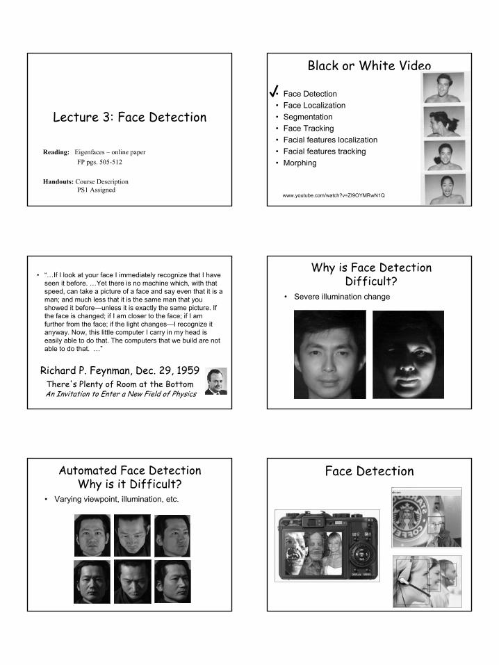
Black or White Video
• Face Detection• Face Localization• Segmentation• Face Tracking• Facial features localization• Facial features tracking• Morphing
www.youtube.com/watch?v=ZI9OYMRwN1Q
Richard P. Feynman, Dec. 29, 1959There's Plenty of Room at the BottomAn Invitation to Enter a New Field of Physics
• “…If I look at your face I immediately recognize that I have seen it before. …Yet there is no machine which, with that speed, can take a picture of a face and say even that it is a man; and much less that it is the same man that you showed it before—unless it is exactly the same picture. If the face is changed; if I am closer to the face; if I am further from the face; if the light changes—I recognize it anyway. Now, this little computer I carry in my head is easily able to do that. The computers that we build are not able to do that. …”
Why is Face Detection Difficult?
• Severe illumination change
• Varying viewpoint, illumination, etc.
Automated Face DetectionWhy is it Difficult?
Face Detection
2
http://bensguide.gpo.gov/3-5/symbols/print/mountrushmore.html
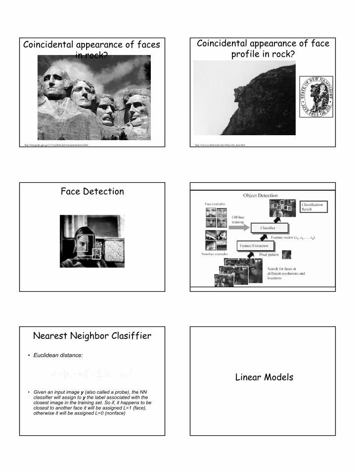
Coincidental appearance of faces in rock?
Coincidental appearance of face profile in rock?
http://www.cs.dartmouth.edu/whites/old_man.html
Face Detection
Nearest Neighbor Clasiffier
• Euclidean distance:
• Given an input image y (also called a probe), the NN classifier will assign to y the label associated with the closest image in the training set. So if, it happens to be closest to another face it will be assigned L=1 (face), otherwise it will be assigned L=0 (nonface)
( )21
212
21 cc yydN
c−= ∑−=
=yy Linear Models
3
1×ℜ∈ kli
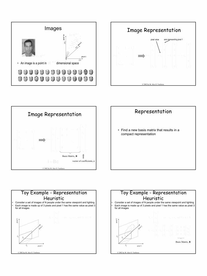
• An image is a point in dimensional space
Images
1 ×ℜ kl
lkI ×ℜ∈ pixel 1
pixe
l kl
pixel 2
2550
255
255 . .
..... .........
. ... ... .
....Image Representation
=
+−
+
klkl
l
l
ii
i
iii
I
1)1(
1
21
.
.
...
....
=
kli
i
i
M
2
1
i
+
+
=
1
0
0
0
0
1
0
0
0
1
21 ML
M
M kliii
© 2002 by M. Alex O. Vasilescu
pixel value axis representing pixel 1
Image Representation
....
=
kli
i
i
MOM
L2
1
10
10
001
Basis Matrix, B
vector of coefficients, c
© 2002 by M. Alex O. Vasilescu
Bci =
=
+−
+
klkl
l
l
ii
i
iii
I
1)1(
1
21
.
.
...
=
kli
i
i
M
2
1
i
Representation
• Find a new basis matrix that results in a compact representation
Toy Example - Representation Heuristic
• Consider a set of images of N people under the same viewpoint and lighting• Each image is made up of 3 pixels and pixel 1 has the same value as pixel 3
for all images
pixel 1
pixel 3
pixe
l 2
Nn1 and .s.t 31
3
2
1
≤≤=
= nn
n
n
n
n ii
i
i
i
i
© 2002 by M. Alex O. Vasilescu
.
i1
i3i2
Toy Example - Representation Heuristic
• Consider a set of images of N people under the same viewpoint and lighting• Each image is made up of 3 pixels and pixel 1 has the same value as pixel 3
for all images
pixel 1
pixel 3
pixe
l 2
...
.............
. ...... .
...
Nn1 and .s.t 31
3
2
1
≤≤=
= nn
n
n
n
n ii
i
i
i
i
+
+
=
1
0
0
0
1
0
0
0
1
321 nnnn iiii
© 2002 by M. Alex O. Vasilescu
.
i1
i3i2
=
ninini
321
100010001
Basis Matrix, B
4
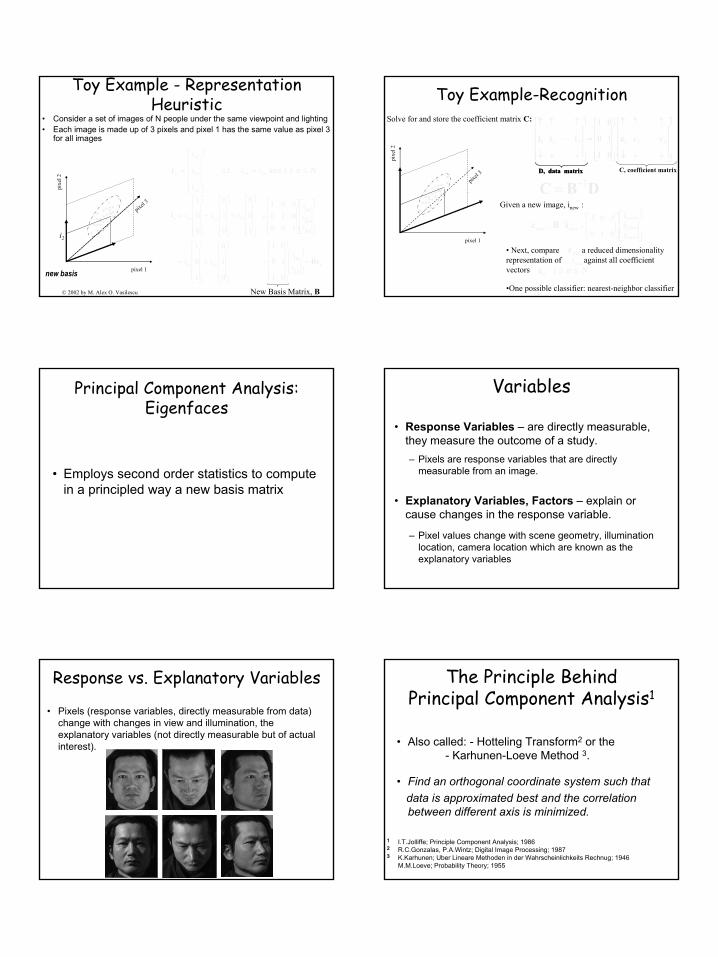
Toy Example - Representation Heuristic
• Consider a set of images of N people under the same viewpoint and lighting• Each image is made up of 3 pixels and pixel 1 has the same value as pixel 3
for all images
pixel 1
pixel 3
pixe
l 2
...
.............
. ...... .
...
Nn1 and .s.t 31
3
2
1
≤≤=
= nn
n
n
n
n ii
i
i
i
i
+
+
=
1
0
0
0
1
0
0
0
1
321 nnnn iiii
+
=
0
1
0
1
0
1
21 nn ii n
nini Bc==
2
1
01
10
01
© 2002 by M. Alex O. Vasilescu
.i2
=
ninini
321
100010001
New Basis Matrix, B
new basis
↓
↑
=
↓
↑
11
01
10
01
ci
D, data matrix
Toy Example-Recognition
pixel 1
pixel 3
pixe
l 2
. ..
.............
. ...... .
...
==
−
new
new
new
newnewiii
3
2
11
010
505 ..iBc
. DBC 1−=
↓↓↓
↑↑↑
=
↓↓↓
↑↑↑
NN ccciii LL 2121
01
10
01
D, data matrix C, coefficient matrix
• Next, compare a reduced dimensionality representation of against all coefficient vectors
•One possible classifier: nearest-neighbor classifier
newcnewiNnn ≤≤1 c
Solve for and store the coefficient matrix C:
Given a new image, inew :
Principal Component Analysis:Eigenfaces
• Employs second order statistics to compute in a principled way a new basis matrix
Variables
• Response Variables – are directly measurable, they measure the outcome of a study. – Pixels are response variables that are directly
measurable from an image.
• Explanatory Variables, Factors – explain or cause changes in the response variable.
– Pixel values change with scene geometry, illumination location, camera location which are known as the explanatory variables
Response vs. Explanatory Variables
• Pixels (response variables, directly measurable from data) change with changes in view and illumination, the explanatory variables (not directly measurable but of actual interest).
The Principle Behind Principal Component Analysis1
• Also called: - Hotteling Transform2 or the - Karhunen-Loeve Method 3.
• Find an orthogonal coordinate system such that data is approximated best and the correlation between different axis is minimized.
1 I.T.Jolliffe; Principle Component Analysis; 19862 R.C.Gonzalas, P.A.Wintz; Digital Image Processing; 19873 K.Karhunen; Uber Lineare Methoden in der Wahrscheinlichkeits Rechnug; 1946
M.M.Loeve; Probability Theory; 1955

5
x1
x2
PCA: Theory
• Define a new origin as the mean of the data set
• Find the direction of maximum variance in the samples (e1) and align it with the first axis (y1),
• Continue this process with orthogonal directions of decreasing variance, aligning each with the next axis
• Thus, we have a rotation which minimizes the covariance.
x1
x2
x
x
x
xx
x x
x
PCA
e1
e2 x
x
xx
xx x
x
y1
y2
...
..............
. ...... .
...
PCA-Dimensionality Reduction• Consider a set of images, & each image is made up of 3 pixels and pixel 1 has the same value
as pixel 3 for all images
• PCA chooses axis in the direction of highest variability of the data, maximum scatter
pixel 1
pixel 3
pixe
l 2
1st axis
2nd axis
[ ] Nn1 and .s.t 31321 ≤≤== nnT
nnnn iiiiii
• Each image is now represented by a vector of coefficients in a reduced dimensionality space.
ninc
=
|||
ccc
|||
Biii NN LL 2121
|||
|||
data matrix, D
D) of (svd TUSVD = UB =set
dentitythat such I BBBSB == TT
TE
• B minimize the following function
The Covariance Matrix• Define the covariance (scatter) matrix of the input samples:
(where µ is the sample mean)
∑=
−−=N
nnnT
1
Tµ)µ)(i(iS
→−←
→−←→−←
↓↓↓−−−↑↑↑
=
µi
µiµi
µiµiµiSN
NT ML
2
1
21
( )( )TMDMDS −−=T [ ]µµM L=where
PCA: Some Properties of the Covariance/Scatter Matrix
• The matrix ST is symmetric
• The diagonal contains the variance of each parameter (i.e. element ST,ii is the variance in the i’th direction).
• Each element ST,ij is the co-variance between the two directions i and j, represents the level of correlation
(i.e. a value of zero indicates that the two dimensions are uncorrelated).
SVD of a Matrix
Scatter of matrix:
( ) ( )M-DVUMD of svdby TΣ=− UB =set
( )( ) ) of (svd 2T
TT SUUMDMD Σ=−−
( )( )TT MDMDS −−=
UB =set
PCA: Goal Revisited
• Look for: - B• Such that:
– [c1 … cN] = BT [i1 … iN]– correlation is mininmized Cov(C) is diagonal
Note that Cov(C) can be expressed via Cov(D) and B :
BSBBMDMDBCC
TT
TTT ))((=
−−=
6
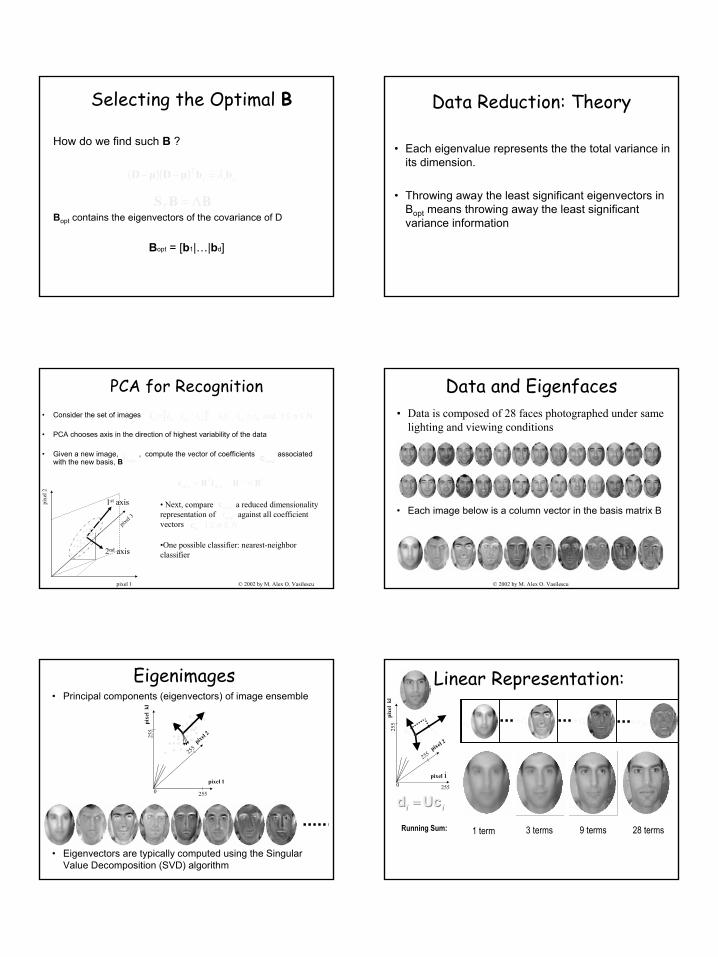
Selecting the Optimal B
How do we find such B ?
Bopt contains the eigenvectors of the covariance of D
Bopt = [b1|…|bd]
BBS Λ=T
iii bbµDµD λ=−− T))((
Data Reduction: Theory
• Each eigenvalue represents the the total variance in its dimension.
• Throwing away the least significant eigenvectors in Bopt means throwing away the least significant variance information
PCA for Recognition• Consider the set of images
• PCA chooses axis in the direction of highest variability of the data
• Given a new image, , compute the vector of coefficients associated with the new basis, B
Tnew
Tnew BBiBc == −1
[ ] Nn1 and .s.t 31321 ≤≤== nnT
nnnn iiiiii
pixel 1
pixel 3
pixe
l 2
1st axis
2nd axis
....
.............
. ...... .
...
newi
• Next, compare a reduced dimensionality representation of against all coefficient vectors
•One possible classifier: nearest-neighbor classifier
newcnewiNnn ≤≤1 c
© 2002 by M. Alex O. Vasilescu
newc
Data and Eigenfaces
• Each image below is a column vector in the basis matrix B
• Data is composed of 28 faces photographed under same lighting and viewing conditions
© 2002 by M. Alex O. Vasilescu
. ..
.... .........
. ... ... .
...• Principal components (eigenvectors) of image ensemble
• Eigenvectors are typically computed using the Singular Value Decomposition (SVD) algorithm
Eigenimages
pixel 1
pixe
l kl
pixel 2
2550
255
255
. .
Linear Representation:
pixel 1
pixe
l kl
pixel 2
2550
255
255 . 3c+1c 9c+ 28c+
2c3c
Running Sum: 1 term 3 terms 9 terms 28 terms
1c
ii Ucd = ii Ucd =
.
7
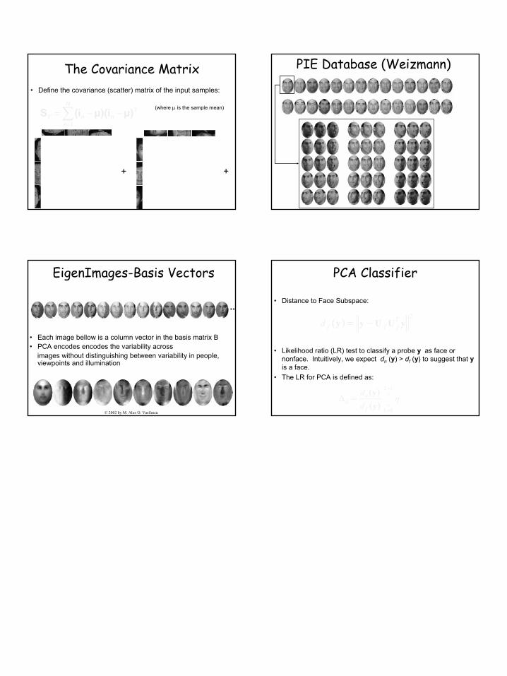
The Covariance Matrix• Define the covariance (scatter) matrix of the input samples:
(where µ is the sample mean)∑=
−−=N
nnnT
1
Tµ)µ)(i(iS
+ +
PIE Database (Weizmann)
EigenImages-Basis Vectors
• Each image bellow is a column vector in the basis matrix B• PCA encodes encodes the variability across
images without distinguishing between variability in people,viewpoints and illumination
© 2002 by M. Alex O. Vasilescu
PCA Classifier
• Distance to Face Subspace:
• Likelihood ratio (LR) test to classify a probe y as face or nonface. Intuitively, we expect dn (y) > df (y) to suggest that yis a face.
• The LR for PCA is defined as:
2)( yUUyy T
fffd −=
η<=
>=
=∆0
1
)()(
L
L
f
nd d
d
y
y