bivariate least squares linear regression: towards a uni ... · bivariate least squares linear...

Applied Mathematical Sciences, Vol. 11, 2017, no. 49, 2393 - 2446HIKARI Ltd, www.m-hikari.com

https://doi.org/10.12988/ams.2017.78260

Bivariate Least Squares Linear Regression:

Towards a Unified Analytic Formalism.

II. Extreme Structural Models

R. Caimmi

Physics and Astronomy Department, Padua University1

Vicolo Osservatorio 3/2, I-35122 Padova, Italy

Copyright c© 2017 R. Caimmi. This is an open access article distributed under the

Creative Commons Attribution License, which permits unrestricted use, distribution, and

reproduction in any medium, provided the original work is properly cited.

Abstract

Concerning bivariate least squares linear regression, the classical re-sults obtained for extreme structural models in earlier attempts [18][11] are reviewed using a new formalism in terms of deviation (matrix)traces which, for homoscedastic data, reduce to usual quantities leavingaside an unessential (but dimensional) multiplicative factor. Within theframework of classical error models, the dependent variable relates tothe independent variable according to a variant of the usual additivemodel. The classes of linear models considered are regression lines inthe limit of uncorrelated errors in X and in Y . The following modelsare considered in detail: (Y) errors in X negligible (ideally null) withrespect to errors in Y ; (X) errors in Y negligible (ideally null) withrespect to errors in X; (C) oblique regression; (O) orthogonal regres-sion; (R) reduced major-axis regression; (B) bisector regression. Forhomoscedastic data, the results are taken from earlier attempts andrewritten using a more compact notation. For heteroscedastic data, theresults are inferred from a procedure related to functional models [30][6]. An example of astronomical application is considered, concerningthe [O/H]-[Fe/H] empirical relations deduced from five samples related

1Affiliated up to September 30th 2014. Current status: Studioso Senior. Current posi-tion: in retirement due to age limits.

2394 R. Caimmi

to different stars and/or different methods of oxygen abundance deter-mination. For low-dispersion samples and assigned methods, differentregression models yield results which are in agreement within the errors(∓σ) for both heteroscedastic and homoscedastic data, while the con-trary holds for large-dispersion samples. In any case, samples related todifferent methods produce discrepant results, due to the presence of (stillundetected) systematic errors, which implies no definitive statement canbe made at present. Asymptotic expressions approximate regression lineslope and intercept variance estimators, for normal residuals, to a betterextent with respect to earlier attempts. Related fractional discrepanciesare not exceeding a few percent for low-dispersion data, which grows upto about 10% for large-dispersion data. An extension of the formalismto generic structural models is left to future work.

Keywords: galaxies: evolution; stars: formation, evolution; methods:data analysis; methods: statistical

1 Introduction

Linear regression is a fundamental and frequently used statistical tool inalmost all branches of science, among which astronomy. The related problemis twofold: regression line slope and intercept estimators are expressed involv-ing minimizing or maximizing some function of the data; on the other hand,regression line slope and intercept variance estimators are expressed requiringknowledge of the error distributions of the data. The complexity mainly arisesfrom the occurrence of intrinsic dispersion in addition to the dispersion relatedto the measurement processes (hereafter quoted as instrumental dispersion),where the distribution corresponding to the former can be different from thedistribution corresponding to the latter i.e. non Gaussian (non normal).

In statistics, problems where the true points have fixed but unknown coor-dinates are called functional regression models, while problems where the truepoints have random (i.e. obeying their own intrinsic distribution) and unknowncoordinates are called structural regression models. Accordingly, functional re-gression models may be conceived as structural regression models where theintrinsic dispersion is negligible (ideally null) with respect to the instrumentaldispersion. Conversely, structural regression models where the instrumentaldispersion is negligible (ideally null) with respect to the intrinsic dispersion,can be defined as extreme structural models [6]. A distinction between func-tional and structural modelling is currently preferred, where the former canbe affected by intrinsic scatter but with no or only minimal assumptions onrelated distributions, while the latter implies (usually parametric) models areplaced on the above mentioned distributions. For further details, an interestedreader is addressed to specific textbooks e.g., [7] Chap. 2 §2.1. In addition,

Bivariate least squares linear regression. II. Extreme structural models 2395

models where the instrumental dispersion is the same from point to point foreach variable, are called homoscedastic models, while models where the in-strumental dispersion is (in general) different from point to point, are calledheteroscedastic models. Similarly, related data are denoted as homoscedasticand heteroscedastic.

In general, problems where the true points lie precisely on an expected linerelate to functional regression models, while problems where the true points are(intrinsically) scattered about an expected line relate to structural regressionmodels e.g., [11] [12].

Bivariate least squares linear regression related to heteroscedastic func-tional models with uncorrelated and correlated errors, following Gaussian dis-tributions, were analysed and formulated in two classical papers [30] [32], whereregression line slope and intercept variance estimators are determined usingthe method of partial differentiation [32]. On the contrary, the method of mo-ments estimator is used to this aim in later attempts e.g., [14] Chap. 1 §1.3.2Eq. (1.3.7) [11].

Bivariate least squares linear regression related to extreme structural mod-els, where the instrumental dispersion is negligible (ideally null) with respectto intrinsic dispersion, was exhaustively treated in two classical papers [18][11] [12] and extended to generic structural models in a later attempt [1].

The above mentioned papers provide the simplest description of linear re-gression. In reality, biases and additional effects must be taken into considera-tion, which implies much more complicated description and formulation, as itcan be seen in specific articles or monographies e.g., [14] [7] [3] [9] [8] [28] [29][21] [16].

Restricting to the astronomical literature, recent investigations [19] [20] areparticularly relevant in that it is the first example (in the field under discus-sion) where linear regression is considered following the modern (since abouthalf a century ago) approach based on likelihoods rather than the old (up toabout a century ago) least-squares approach. More specifically, a hierarchicalmeasurement error model is set up therein, the complicated likelihood is writ-ten down, and a variety of minimum least-squares and Bayesan solutions areshown, which can treat functional, structural, multivariate, truncated and cen-sored mesaurement error regression problems. Additional statistical applica-tions to astronomical and astrophysical data can be found in current literaturee.g., [13] [17].

Even in dealing with the simplest homoscedastic (or heteroscedastic) func-tional and structural models, still no unified analytic formalism has been de-veloped (to the knowledge of the author) where (i) structural heteroscedasticmodels with instrumental and intrinsic dispersion of comparable order in bothvariables, are considered; (ii) previous results are recovered in the limit of dom-inant instrumental dispersion; and (iii) previous results are recovered in the

2396 R. Caimmi

limit of dominant intrinsic dispersion. A related formulation may be usefulalso for computational methods, in the sense that both the general case andlimiting situations can be described by a single numerical code.

A first step towards a unified analytic formalism of bivariate least squareslinear regression involving functional models has been performed in an earlierattempt [6], where the least-squares approach developed in two classical papers[30] [32] has been reviewed and reformulated by definition and use of deviation(matrix) traces. The current investigation aims at making a second step alongthe same direction, in dealing with extreme structural models.

More specifically, the results found in two classical papers [18] [11] [12] shallbe reformulated in terms of deviation traces for homoscedastic models, andextended to the general case of heteroscedastic models by analogy with theircounterparts related to functional models, within the framework of classicalerror models where the dependent variable relates to the independent variableaccording to a variant of the classical additive error model.

In this view, homoscedastic structural models are conceived as modelswhere both the instrumental and the intrinsic dispersion are the same frompoint to point. Conversely, models where the instrumental and/or the intrin-sic dispersion are (in general) different from point to point, are conceived asheteroscedastic structural models.

Regression line slope and intercept estimators, and related variance esti-mators, are expressed in terms of deviation traces for different homoscedasticmodels [18] [11] [12] in section 2, where an extension to corresponding het-eroscedastic models is also performed, and both normal and non normal resid-uals are considered. An example of astronomical application is outlined insection 3. The discussion is presented in section 4. Finally, the conclusion isshown in section 5. Some points are developed with more detail in the Ap-pendix. An extension of the formalism to generic structural models is left tofuture work.

2 Least-squares fitting of a straight line

2.1 General considerations

Attention shall be restricted to the classical problem of least-squares fittingof a straight line, where both variables are measured with errors. Without lossof generality, structural models can be conceived as related to an ideal situationwhere the variables obey a linear relation, as:

y∗i = ax∗i + b ; 1 ≤ i ≤ n ; (1)

in connection with true points, P∗i ≡ (x∗i , y∗i ), 1 ≤ i ≤ n. The occurrence

of random (measure independent) processes makes true points shift outside


or along the ideal straight line, inferred from Eq. (1), towards actual points,P∗Si ≡ (xSi, ySi). The occurrence of mesaurement processes makes the actualpoints shift towards the observed points, Pi ≡ (Xi, Yi).

In this view, the least squares fitting of a straight line is conceptually similarfor functional (in absence of intrinsic scatter) and structural (in presence ofintrinsic scatter) models: “What is the best line fitting to a sample of observedpoints, Pi, 1 ≤ i ≤ n?” It is worth noticing the correspondence between truepoints, P∗i , and observed points, Pi, is not one-to-one unless it is assumed allpoints are shifted along the same direction. More specifically, two observedpoints, Pi, Pj, of equal coordinates, (Xi, Yi) = (Xj, Yj), relate to true points,P∗i , P

∗j , of (in general) different coordinates, (x∗i , y

∗i ) 6= (x∗j , y

∗j ), both in presence

and in absence of intrinsic scatter. The least-square estimator and the lossfunction have the same formal expression for functional and structural models,but in the latter case the “statistical distances” e.g., [14] Chap. 1 §1.3.3 dependon the total (instrumental + intrinsic) scatter.

The observed points and the actual points are related as:

Zi = zSi + (ξFz)i ; Z = X, Y ; z = x, y ; 1 ≤ i ≤ n ; (2)

where (ξFx)i, (ξFy)i, are the instrumental (i.e. due to the intrumental scatter)errors on xSi, ySi, respectively, assumed to obey Gaussian distributions withnull expectation values and known variances, [(σxx)F]i, [(σyy)F]i, and covari-ance, [(σxy)F]i.

The actual points and the true points on the ideal straight line are relatedas:

zSi = z∗i + (ξSz)i ; z = x, y; 1 ≤ i ≤ n ; (3)

where (ξSx)i, (ξSy)i, are the intrinsic (i.e. due to the intrinsic scatter) errors onx∗i , y

∗i , respectively, assumed to obey specified distributions with null expecta-

tion values and finite variances, [(σxx)S]i, [(σyy)S]i, and covariance, [(σxy)S]i.The observed points and the true points on the ideal straight line are related

as:

Zi = z∗i + ξzi ; Z = X, Y ; z = x, y ; 1 ≤ i ≤ n ; (4)

where the (instrumental + intrinsic) errors, ξxi, ξyi , are defined as:

ξzi = (ξFz)i + (ξSz)i ; z = x, y ; 1 ≤ i ≤ n ; (5)

which obey specified distributions with null expectation values and finite vari-ances, (σxx)i, (σyy)i, and covariance, (σxy)i. The further restriction that (ξFz)i,(ξSz)i, z = x, y, 1 ≤ i ≤ n, are independent, implies the relation [1]:

(σzz)i = [(σzz)F]i + [(σzz)S]i ; (σxy)i = [(σxy)F]i + [(σxy)S]i ; (6)

2398 R. Caimmi

where the intrinsic covariance matrixes are unknown and must be assigned orestimated, which will be supposed in the following.

Then the error model is defined by Eqs. (1)-(6), where both instrumentalerrors, (ξFz)i, and intrinsic errors, (ξSz)i, are assumed to be independent of truevalues, z∗i , for given instrumental covariance matrixes, (ΣF)i = || [(σxy)F]i ||,intrinsic covariance matrixes, (ΣS)i = || [(σxy)S]i ||, respectively, and (total)covariance matrixes, Σi = || (σxy)i ||, hence Σi = (ΣF)i + (ΣS)i, 1 ≤ i ≤ n. Itmay be considered as a variant of the classical additive error model e.g., [1] [7]Chap. 1 §1.2 Chap. 3 §3.2.1 [19] [20] [3] Chap. 4 §4.3.

In the case under discussion, the regression estimator minimizes the lossfunction, defined as the sum (over the n observations) of squared residualse.g., [32] or statistical distances of the observed points, Pi ≡ (Xi, Yi), fromthe estimated line in the unknown parameters, a, b, x1, ..., xn e.g., [14] Chap. 1§1.3.3. Under restrictive assumptions, the regression estimator is the functionalmaximum likelihood estimator e.g., [7] Chap. 3 §3.4.2.

The coordinates, (xi, yi), may be conceived as the adjusted values of relatedobservations, (Xi, Yi), on the estimated regression line [30] [32] and, in addition,as estimators of the coordinates, (x∗i , y

∗i ), on the true regression line i.e. the

ideal straight line. The line of adjustment, PiPi e.g., [32] may be conceivedas an estimator of the statistical distance, PiP∗i e.g., [14] Chap. 1 §1.3.3 wherePi(xi, yi) is the adjusted point on the estimated regression line:

yi = axi + b ; 1 ≤ i ≤ n ; (7)

where, in general, estimators are denoted by hats, and P∗i (x∗i , y∗i ) is the true

point on the ideal straight line, Eq. (1).To the knowledge of the author, only classical error models are considered

for astronomical applications, and for this reason different error models suchas Berkson models and mixture error models e.g., [7] Chap. 3 Sect. 3.2 shallnot be dealt with in the current attempt. From this point on, investigationshall be limited to extreme structural models and least-squares regression es-timators for the following reasons. First, they are important models in theirown right, furnishing an approximation to real world situations. Second, acareful examination of these simple models helps for understanding the theo-retical underpinnings of methods for other models of greater complexity suchas hierarchical models e.g., [19] [20].

2.2 Extreme structural models

With regard to extreme structural models, bivariate least squares linearregression were analysed in two classical papers in the special case of obliqueregression i.e. constant variance ratio, (σyy)i/(σxx)i = c2, 1 ≤ i ≤ n, and con-stant correlation coefficients, ri = r, 1 ≤ i ≤ n. More specifically, orthogonal


(c2 = 1) and oblique regression were analysed in the earlier [18] and in thelatter [11] [12] paper, respectively. In absence of additional information, ho-moscedastic models are used [18] unless the intrinsic dispersion is estimated [1],from which related weights may be determined and the least squares estimatortogether with the loss function may be expressed for both homoscedastic andheteroscedastic models [1] [20].

The (dimensionless) squared weighted residuals can be defined as in thecase of functional models [32]:

(Ri)2 =

wxi(Xi − xi)2 + wyi(Yi − yi)2 − 2ri

√wxi

wyi(Xi − xi)(Yi − yi)1− r2i

; (8a)

ri =(σxy)i

[(σxx)i(σyy)i]1/2; |ri| ≤ 1 ; 1 ≤ i ≤ n ; (8b)

where wxi, wyi , are the weights of the various measurements (or observations)

and ri the correlation coefficients. The terms, wxi(Xi − xi)2, wyi(Yi − yi)2, ri,

1 ≤ i ≤ n, are dimensionless by definition. An equivalent formulation in matrixformalism can be found in specific textbooks, where weighted true residualsare conceived as (dimensionless) “statistical distances” from data points torelated points on the regression line e.g., [14] Chap. 1 §1.3.3 Eq. (1.3.16).

Accordingly, the least-squares regression estimator and the loss functioncan be expressed as in the case of functional models [6] but the weights, wxi

,wyi , and the correlation coefficients, ri, are related to intrinsic scatter insteadof instrumental scatter. Then the regression line slope and intercept estimatorstake the same formal expression with respect to their counterparts related tofunctional models, while (in general) the contrary holds for regression line slopeand intercept variance estimators.

Classical results on extreme structural models [18] [11] [12] are restricted tooblique regression for homoscedastic data with constant correlation coefficients(wxi

= wx, wyi = wy, ri = r, 1 ≤ i ≤ n). In the following subsections, theabove mentioned results extended to heteroscedastic data shall be expressedin terms of weighted deviation (matrix) traces [6]:

Qpq =n∑

i=1

Qi(wxi, wyi , ri)(Xi − X)p(Yi − Y )q ; (9)

Q00 =n∑

i=1

Qi(wxi, wyi , ri) = nQ ; (10)

where Qpq are the (weighted) pure (p = 0 and/or q = 0) and mixed (p > 0 and

2400 R. Caimmi

q > 0) deviation traces, and X, Y , are weighted means:

Z =

n∑i=1

WiZi

n∑i=1

Wi

; Z = X, Y ; (11)

Wi =wxi

Ω2i

1 + a2Ω2i − 2ariΩi

; 1 ≤ i ≤ n ; (12)

Ωi =

√wyi

wxi

; 1 ≤ i ≤ n ; (13)

in the limit of homoscedastic data with equal correlation coefficients, wxi= wx,

wyi = wy, ri = r, 1 ≤ i ≤ n, which implies Qi(wxi, wyi , ri) = Q(wx, wy, r) = Q,

Eqs. (9), (10), (11), (12), and (13) reduce to:

Qpq = QSpq ; (14)

Spq =n∑

i=1

(Xi −X)p(Yi − Y )q ; (15)

Q00 = QS00 ; (16)

S00 = n ; (17)

Z = Z ; Z = X, Y ; (18)

Wi = W =wxΩ2

1 + a2Ω2 − 2arΩ; 1 ≤ i ≤ n ; (19)

Ωi = Ω =

√wy

wx

; 1 ≤ i ≤ n ; (20)

where Spq are the (unweighted) pure (p = 0 and/or q = 0) and mixed (p > 0and q > 0) deviation traces.

Turning to the general case and using the weighted squared error loss func-tion, T

R=∑n

i=1(Ri)2, yields for regression line slope and intercept estima-

tors the same expression with respect to functional models [6]. Accordingly,regression line slope and intercept estimators may be conceived similarly tostate functions in thermodynamics: for an assigned true point, P∗i ≡ (x∗i , y

∗i ),

what is relevant is the related observed point, Pi ≡ (Xi, Yi), regardless of thepath followed via instrumental and/or intrinsic scatter. More specifically, theregression line intercept estimator obeys the equation e.g., [32] [6]:

b = Y − aX ; (21)

which implies the “barycentre” of the data, P ≡ (X, Y ), lies on the estimatedregression line, inferred from Eq. (7), and the regression line slope estimator is


one among three real solutions of a pseudo cubic equation or two real solutionsof a pseudo quadratic equation, where the coefficients are weakly dependenton the unknown slope. For further details, an interested reader is addressed toearlier attempts [30] [32] [6]. The above mentioned equations have the sameformal expression for functional and structural models, which also holds forthe regression line slope and intercept estimators.

The regression line slope and intercept variance estimators for functionalmodels, calculated using the method of partial differentiation e.g., [32] andthe method of moments estimators e.g., [14] Chap. 1 §1.3.2 Eq. (1.3.7) yield, ingeneral, different results [6]. The same is expected to hold, a fortiori, for struc-tural models, for which the method of moments estimators and the δ-methodhave been exploited in classical investigations e.g., [18] [11] [12]. Accordingly,related results shall be considered and expressed in terms of unweighted de-viation traces for homoscedastic data with equal correlation coefficients andextended in terms of weighted deviation traces for heteroscedastic data, withregard to a number of special cases considered in earlier attempts in the limitof uncorrelated errors in X and in Y [18] [11] [12]. With this restriction, thepseudo cubic equation reduces to:

V20a3 − 2V11a

2 − (W20 − V02)a+ W11 = 0 ; (22)

where the deviation traces are defined by Eq. (9), via Eq. (12) and Vi =W 2

i /wxi. For further details, an interested reader is addressed to the par-

ent paper [30] and to a recent attempt [6]. A formulation of Euclidean andstatistical squared residual sum for homoscedastic and heteroscedastic data isexpressed in Appendix A.

2.3 Errors in X negligible with respect to errors in Y

In the limit of errors in X negligible with respect to errors in Y , a2(σxx)i (σyy)i, a(σxy)i (σyy)i, 1 ≤ i ≤ n. Ideally, (σxx)i → 0, (σxy)i → 0, 1 ≤ i ≤ n,which implies ri → 0, wxi

→ +∞, Ωi → 0, Wi → wyi , 1 ≤ i ≤ n. Accordingly,the errors in X and in Y are uncorrelated.

For homoscedastic data, wxi= wx, wyi = wy, 1 ≤ i ≤ n, the regression line

slope and intercept estimators are [18] [6]:

aY =S11

S20

; (23)

bY = Y − aYX ; (24)

where the index, Y, stands for OLS(Y|X) i.e. ordinary least square regressionor, in general, WLS(Y|X) i.e. weighted least square regression of the dependentvariable, Y , against the independent variable, X [18]. Accordingly, relatedmodels shall be quoted as Y models.

2402 R. Caimmi

The regression line slope and intercept variance estimators, in the specialcase of normal residuals may be calculated using different methods and/ormodels e.g., [14] Chap. 1 §1.3.2 Eq. (1.3.7) [11] [12] [6]. The result is:

[(σaY)N]2 =(aY)2

n− 2

[(n− 2)RY

aYS11

+ Θ(aY, aY, aX)

]

=(aY)2

n− 2

[aX − aYaY

+ Θ(aY, aY, aX)

]; (25)

[(σbY)N]2 =[

1

aY

S11

S00

+ (X)2]

[(σaY)N]2 − aYn− 2

S11

S00

Θ(aY, aY, aX) ; (26)

where the index, N, denotes normal residuals, R is defined in Appendix A, andaX = S02/S11. The funcion, Θ(aY, aY, aX), is a special case of a more generalfunction, Θ(aC, aY, aX) which, in turn, depends on the method and/or modelused. For further details, an interested reader is addressed to Appendix B.

The regression line slope and intercept variance estimators, in the generalcase of non normal residuals may be calculated using the δ-method [18]. Theresult is:

(σaY)2 =S22 + (aY)2S40 − 2aYS31

(S20)2; (27)

(σbY)2 =aYn

aX − aYaY

S11

S00

+ (X)2(σaY)2 − 2

nXσbYaY

; (28)

σbYaY=S12 + (aY)2S30 − 2aYS21

S20

; (29)

where Eqs. (27)-(29) are equivalent to their counterparts expressed in the par-ent paper [18].

The application of the δ-method provides asymptotic formulae which un-derstimate the true regression coefficient uncertainty in samples with low(n

<∼ 50) or weakly correlated population [11] [12]. In the special case ofnormal and data-independent residuals, Θ(aY, aY, aX) → 0, Eqs. (27), (28),must necessarily reduce to (25), (26), respectively, which implies an additionalfactor, n/(n−2), in the first term on the right-hand side of Eqs. (27)-(29). Forfurther details, an interested reader is addressed to Appendix C.

The expression of the regression line slope and intercept estimators andrelated variance estimators for normal residuals, Eqs. (23), (24), (25), (26),coincide with their counterparts determined for Y models in classical and recentattempts e.g., [11] [12] Eq. (4) in the limit c2 = σyy/σxx → +∞ [22] Eqs. (3)-(7).

For heteroscedastic data, the regression line slope and intercept estimatorsare [6]:

aY =(wy)11(wy)20

; (30)


bY = Y − aYX ; (31)

where the weighted means, X and Y , are defined by Eqs. (11)-(13).For functional models, regression line slope and intercept variance estima-

tors in the general case of heteroscedastic data reduce to their counterpartsin the special case of homoscedastic data, as σaY [(wy)pq]2 → [σaY(wySpq)]

2,σbY [(wy)pq]2 → [σbY(wySpq)]

2, via Eq. (9) where Qi = (wy)i = wy, 1 ≤ i ≤ n.For further details, an interested reader is addressed to an earlier attempt [6].

Under the assumption that the same holds for extreme structural models,Eqs. (25)-(29) take the general expression:

[(σaY)N]2 =(aY)2

n− 2

[n− 2

n

RY

aY

(wy)00(wy)11

+ Θ(aY, aY, a′X)

]

=(aY)2

n− 2

[a′X − aYaY

+ Θ(aY, aY, a′X)

]; (32)

[(σbY)N]2 =

[1

aY

(wy)11(wy)00

+ (X)2]

[(σaY)N]2 − aYn− 2

(wy)11(wy)00

Θ(aY, aY, a′X) ; (33)

(σaY)2 =(wy)00n

(wy)22 + (aY)2(wy)40 − 2aY(wy)31[(wy)20]2

; (34)

(σbY)2 =aYn

a′X − aYaY

(wy)11(wy)00

+ (X)2(σaY)2 − 2

nXσbYaY

; (35)

σbYaY=

(wy)12 + (aY)2(wy)30 − 2aY(wy)21(wy)20

; (36)

where a′X = (wy)02/(wy)11, R is defined in Appendix A and Θ is expressed interms of n(wy)pq/(wy)00 instead of Spq.

In the special case of normal and data-independent residuals, Θ(aY, aY, a′X)→

0, Eqs. (34), (35), must necessarily reduce to (32), (33), respectively, which im-plies an additional factor, n/(n − 2), in the first term on the right-hand sideof Eqs. (34)-(36).

In absence of a rigorous proof, Eqs. (32)-(36) must be considered as ap-proximate results.

2.4 Errors in Y negligible with respect to errors in X

In the limit of errors in Y negligible with respect to errors in X, (σyy)i a2(σxx)i, (σxy)i a(σxx)i, 1 ≤ i ≤ n. Ideally, (σyy)i → 0, (σxy)i → 0,1 ≤ i ≤ n, which implies ri → 0, wyi → +∞, Ωi → +∞, Wi → wxi

, 1 ≤ i ≤ n.Accordingly, the errors in X and in Y are uncorrelated. As outlined in anearlier paper [6], the model under discussion can be related to the inverseregression, which has a large associate literature e.g., [23] [15] [24] [2] [22].

2404 R. Caimmi


slope and intercept estimators are [18] [6]:

aX =S02

S11

; (37)

bX = Y − aXX ; (38)

where the index, X, stands for OLS(X|Y) i.e. ordinary least square regressionor, in general, WLS(X|Y) i.e. weighted least square regression of the dependentvariable, X, against the independent variable, Y [18]. Accordingly, relatedmodels shall be quoted as X models.


[(σaX)N]2 =(aX)2

n− 2

[(n− 2)RX

aXS11

+ Θ(aX, aY, aX)

]

=(aX)2

n− 2

[aX − aYaY

+ Θ(aX, aY, aX)

]; (39)

[(σbX)N]2 =[

1

aX

S11

S00

+ (X)2]

[(σaX)N]2 − aXn− 2

S11

S00

Θ(aX, aY, aX) ; (40)

where the index, N, denotes normal residuals, R is defined in Appendix A, andaY = S11/S20. The funcion, Θ(aX, aY, aX), is a special case of a more generalfunction, Θ(aC, aY, aX) which, in turn, depends on the method and/or modelused. For further details, an interested reader is addressed to Appendix B.

The regression line slope and intercept variance estimators, in the generalcase of non normal residuals may be calculated using the δ-method [18]. Theresult is:

(σaX)2 =S04 + (aX)2S22 − 2aXS13

(S11)2; (41)

(σbX)2 =aXn

aX − aYaY

S11

S00

+ (X)2(σaX)2 − 2

nXσbXaX

; (42)

σbXaX=S03 + (aX)2S21 − 2aXS12

S11

; (43)

where Eqs. (41)-(43) are equivalent to their counterparts expressed in the par-ent paper [18].


<∼ 50) or weakly correlated population [11] [12]. In the special case ofnormal and data-independent residuals, Θ(aX, aY, aX) → 0, Eqs. (41), (42),


must necessarily reduce to (39), (40), respectively, which implies an additionalfactor, n/(n−2), in the first term on the right-hand side of Eqs. (41)-(43). Forfurther details, an interested reader is addressed to Appendix C.


aX =(wx)02(wx)11

; (44)

bX = Y − aXX ; (45)

where the weighted means, X and Y , are defined by Eqs. (11)-(13).

For functional models, regression line slope and intercept variance estima-tors in the general case of heteroscedastic data reduce to their counterpartsin the special case of homoscedastic data, as σaX [(wx)pq]2 → [σaX(wxSpq)]

2,σbX [(wx)pq]2 → [σbX(wxSpq)]

2, via Eq. (9) where Qi = (wx)i = wx, 1 ≤ i ≤ n.For further details, an interested reader is addressed to an earlier attempt [6].


[(σaX)N]2 =(aX)2

n− 2

[n− 2

n

RX

aX

(wx)00(wx)11

+ Θ(aX, a′Y, aX)

]

=(aX)2

n− 2

[aX − a′Ya′Y

+ Θ(aX, a′Y, aX)

]; (46)

[(σbX)N]2 =

[1

aX

(wx)11(wx)00

+ (X)2]

[(σaX)N]2 − aXn− 2

(wx)11(wx)00

Θ(aX, a′Y, aX) ; (47)

(σaX)2 =(wx)00n

(wx)04 + (aX)2(wx)22 − 2aX(wx)13[(wx)11]2

; (48)

(σbX)2 =aXn

aX − a′Ya′Y

(wx)11(wx)00

+ (X)2(σaX)2 − 2

nXσbXaX

; (49)

σbXaX=

(wx)03 + (aX)2(wx)21 − 2aX(wx)12(wx)11

; (50)

where a′Y = (wx)11/(wx)20, R is defined in Appendix A, and Θ is formulatedin terms of n(wx)pq/(wx)00 instead of Spq.

In the special case of normal and data-independent residuals, Θ(aX, a′Y, aX)→

0, Eqs. (48), (49), must necessarily reduce to (46), (47), respectively, which im-plies an additional factor, n/(n − 2), in the first term on the right-hand sideof Eqs. (48)-(50).


2406 R. Caimmi

2.5 Oblique regression

In the limit of constant y to x variance ratios and constant correlationcoefficients, the following relations hold:

(σyy)i(σxx)i

= c2 ;wxi

wyi

= Ω−2i = c2 ;(σxy)i(σxx)i

= ric = rc ; 1 ≤ i ≤ n ; (51)

Wi =wxi

a2 + c2 − 2rac; 1 ≤ i ≤ n ;

(wy)pq(wy)rs

=(wx)pq(wx)rs

; (52)

where the weights are assumed to be inversely proportional to related variances,wzi ∝ 1/(σzz)i, z = x, y, as usually done e.g., [11] [12]. By definition, c hasthe dimensions of a slope, which highly simplifies dimension checks throughoutequations, and for this reason it has been favoured with respect to differentchoices exploited in earlier attempts e.g., [30] [14] Chap. 1 §1.3 [11] [12].

It is worth noticing that Eq. (51) holds for both homoscedastic and het-eroscedastic data. It can be seen that the lines of adjustment are orientedalong the same direction [31] but are perpendicular to the regression line onlyin the special case of orthogonal regression, c2 = 1 e.g., [7] Chap. 3 §3.4.2.Accordingly, the term “oblique regression” has been preferred with respect to“generalized orthogonal regression” used in an earlier attempt [6].

The variance ratio, c2, may be expressed in terms of instrumental andintrinsic variance ratios, c2F, and c2S, respectively, as:

c2 =[(σxx)i]F(σxx)i

c2F +[(σxx)i]S(σxx)i

c2S ; 1 ≤ i ≤ n ; (53a)

c2F =[(σyy)i]F[(σxx)i]F

; c2S =[(σyy)i]S[(σxx)i]S

; 1 ≤ i ≤ n ; (53b)

where c2F = c2S implies c2F = c2S = c2; c2 → c2F for functional models, [(σzz)i]S [(σzz)i]F, z = x, y, 1 ≤ i ≤ n; c2 → c2S for extreme structural models,[(σzz)i]F [(σzz)i]S, z = x, y, 1 ≤ i ≤ n.


slope and intercept estimators are [11] [12] [6]:

aC =S02 − c2S20

2S11

1∓

1 + c2(S02 − c2S20

2S11

)−21/2

=aXaY − c2

2aY

1∓

1 + c2(aXaY − c2

2aY

)−21/2 ; (54)

bC = Y − aCX ; (55)

where the index, C, denotes oblique regression, aY = S11/S20; aX = S02/S11;and the double sign corresponds to the solutions of a second-degree equation,


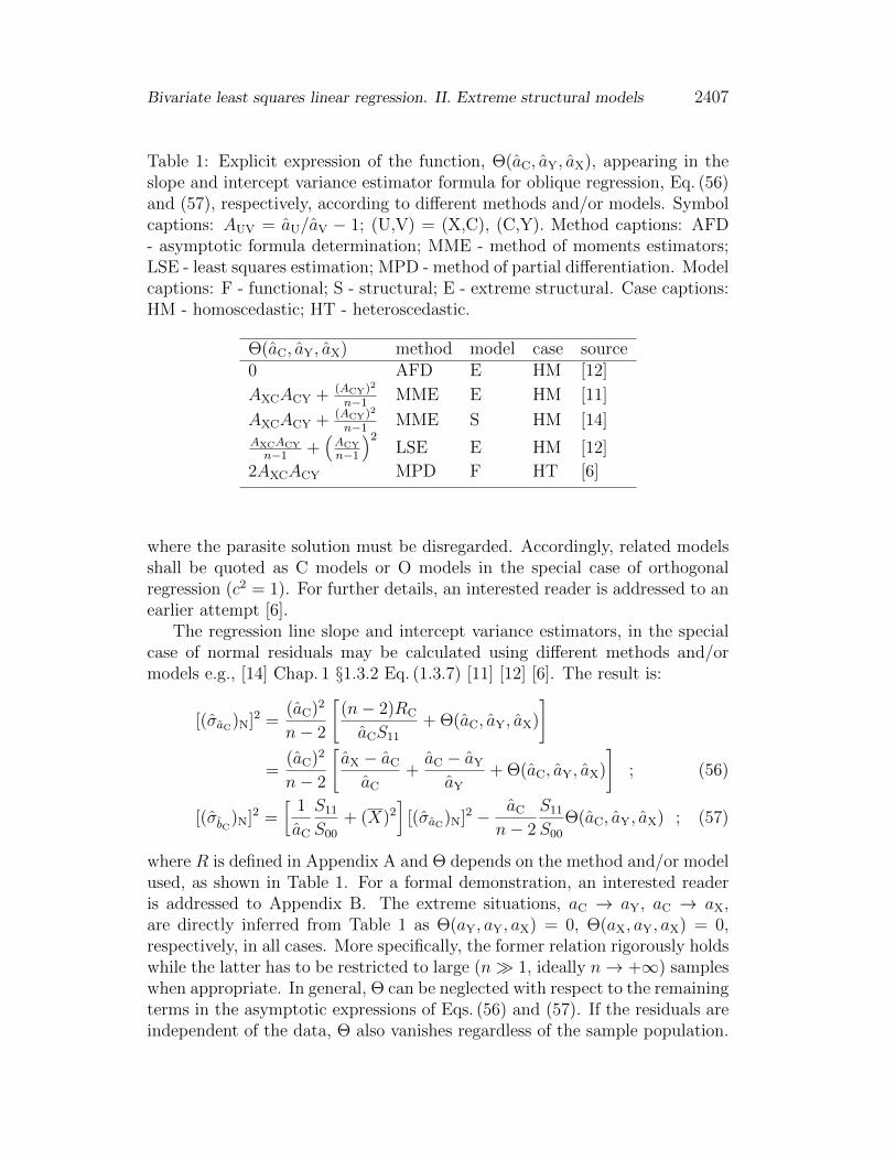
Table 1: Explicit expression of the function, Θ(aC, aY, aX), appearing in theslope and intercept variance estimator formula for oblique regression, Eq. (56)and (57), respectively, according to different methods and/or models. Symbolcaptions: AUV = aU/aV − 1; (U,V) = (X,C), (C,Y). Method captions: AFD- asymptotic formula determination; MME - method of moments estimators;LSE - least squares estimation; MPD - method of partial differentiation. Modelcaptions: F - functional; S - structural; E - extreme structural. Case captions:HM - homoscedastic; HT - heteroscedastic.

Θ(aC, aY, aX) method model case source0 AFD E HM [12]

AXCACY + (ACY)2

n−1 MME E HM [11]

AXCACY + (ACY)2

n−1 MME S HM [14]AXCACY

n−1 +(ACY

n−1

)2LSE E HM [12]

2AXCACY MPD F HT [6]

where the parasite solution must be disregarded. Accordingly, related modelsshall be quoted as C models or O models in the special case of orthogonalregression (c2 = 1). For further details, an interested reader is addressed to anearlier attempt [6].


[(σaC)N]2 =(aC)2

n− 2

[(n− 2)RC

aCS11

+ Θ(aC, aY, aX)

]

=(aC)2

n− 2

[aX − aCaC

+aC − aYaY

+ Θ(aC, aY, aX)

]; (56)

[(σbC)N]2 =[

1

aC

S11

S00

+ (X)2]

[(σaC)N]2 − aCn− 2

S11

S00

Θ(aC, aY, aX) ; (57)

where R is defined in Appendix A and Θ depends on the method and/or modelused, as shown in Table 1. For a formal demonstration, an interested readeris addressed to Appendix B. The extreme situations, aC → aY, aC → aX,are directly inferred from Table 1 as Θ(aY, aY, aX) = 0, Θ(aX, aY, aX) = 0,respectively, in all cases. More specifically, the former relation rigorously holdswhile the latter has to be restricted to large (n 1, ideally n→ +∞) sampleswhen appropriate. In general, Θ can be neglected with respect to the remainingterms in the asymptotic expressions of Eqs. (56) and (57). If the residuals areindependent of the data, Θ also vanishes regardless of the sample population.

2408 R. Caimmi

For further details, an interested reader is addressed to Appendix B and C.The regression line slope and intercept variance estimators, in the general

case of non normal residuals, may be calculated using the δ-method [18] [11][12]. The result is:

(σaC)2 = (aC)2c4(σaY)2 + (aY)4(σaX)2 + 2(aY)2c2σaYaX

(aY)2[4(aY)2c2 + (aYaX − c2)2]; (58)

(σbC)2 =aCn

[aX − aCaC

+aC − aYaY

]S11

S00

+ (X)2(σaC)2

− 2

nX(σbYaC

+ σbXaC) ; (59)

σaYaX =S13 + aYaXS31 − (aY + aX)S22

S20S11

; (60)

σbYaC=

aCc2

aY[4(aY)2c2 + (aYaX − c2)2]1/2S12 + aYaCS30 − (aY + aC)S21

S20

; (61)

σbXaC=

aCaY[4(aY)2c2 + (aYaX − c2)2]1/2

S03 + aXaCS21 − (aX + aC)S12

S11

; (62)

where Eqs. (58) and (59) in the special case, c2 = 1, are equivalent to theircounterparts expressed in the parent paper [18] provided absolute values ap-pearing therein are removed. For a formal discussion, an interested reader isaddressed to Appendix D. In addition, Eq. (58) is equivalent to its counterpartexpressed in the parent paper [11] [12].

The dependence on the variance ratio, c2, in Eqs. (58), (61), (62), may beeliminated via Eq. (142), Appendix B. The result is:

(σaC)2 = (aC)2

×(aC)4(AXC)2(σaY)2 + (aY)4(ACY)2(σaX)2 + 2(aY)2(aC)2AXCACYσaYaX

(aY)24(aY)2(aC)2AXCACY + [aYaXACY − (aC)2AXC]2; (63)

σbYaC=

(aC)3AXC

aY4(aY)2(aC)2AXCACY + [(aYaXACY − (aC)2AXC]21/2

× S12 + aYaCS30 − (aY + aC)S21

S20

; (64)

σbXaC=

aCaYACY

4(aY)2(aC)2AXCACY + [(aYaXACY − (aC)2AXC]21/2

× S03 + aXaCS21 − (aX + aC)S12

S11

; (65)

AUV =aUaV− 1 ; (U,V) = (X,C), (C,Y), (X,Y) ; (66)

in terms of slope estimators, variance slope estimators, and deviation traces.



<∼ 50) or weakly correlated population [11] [12]. In the special case ofnormal and data-independent residuals, Θ(aC, aY, aX) → 0, Eqs. (58), (59),must necessarily reduce to (56), (57), respectively, which implies an additionalfactor, n/(n−2), in the first term on the right-hand side of Eqs. (27), (41), and(59)-(62). For further details, an interested reader is addressed to AppendixC.


aC =(wx)02 − c2(wx)20

2(wx)11

1∓

1 + c2(

(wx)02 − c2(wx)202(wx)11

)−21/2

=aXa

′Y − c2

2a′Y

1∓

1 + c2(aXa

′Y − c2

2a′Y

)−21/2 ; (67)

bC = Y − aCX ; (68)

where a′Y = (wx)11/(wx)20; aX = (wx)02/(wx)11; and the weighted means, X,Y , are defined by Eqs. (11)-(13).

For functional models, regression line slope and intercept variance estima-tors in the general case of heteroscedastic data reduce to their counterpartsin the special case of homoscedastic data, as σaC [(wx)pq]2 → [σaC(wxSpq)]

2,σbC [(wx)pq]2 → [σbC(wxSpq)]

2, via Eq. (9) where Qi = (wx)i = wx, 1 ≤ i ≤ n.For further details, an interested reader is addressed to an earlier attempt [6].


[(σaC)N]2 =(aC)2

n− 2

[n− 2

n

RC

aC

(wx)00(wx)11

+ Θ(aC, a′Y, aX)

]

=(aC)2

n− 2

[aX − aCaC

+aC − a′Ya′Y

+ Θ(aC, a′Y, aX)

]; (69)

[(σbC)N]2 =

[1

aC

(wx)11(wx)00

+ (X)2]

[(σaC)N]2 − aCn− 2

(wx)11(wx)00

Θ(aC, a′Y, aX) ; (70)

(σaC)2 = (aC)2c4(σaY)2 + (aY)4(σaX)2 + 2(aY)2c2σaYaX

(aY)2[4(aY)2c2 + (aYaX − c2)2]; (71)

(σbC)2 =aCn

[aX − aCaC

+aC − a′Ya′Y

](wx)11(wx)00

+ (X)2(σa′C)2

− 2

nX(σbYaC

+ σbXaC) ; (72)

2410 R. Caimmi

σaYaX =(wx)00n

(wx)13 + aYaX(wx)31 − (aY + aX)(wx)22(wx)20(wx)11

; (73)

σbYaC=

aCc2

aY[4(aY)2c2 + (aYaX − c2)2]1/2

× (wx)12 + aYaC(wx)30 − (aY + aC)(wx)21(wx)20

; (74)

σbXaC=

aCaY[4(aY)2c2 + (aYaX − c2)2]1/2

× (wx)03 + aXaC(wx)21 − (aX + aC)(wx)12(wx)11

; (75)

(σaC)2 = (aC)2

×(aC)4(AXC)2(σaY)2 + (aY)4(ACY′)2(σaX)2 + 2(aY)2(aC)2AXCACY′σaYaX

(aY)24(aY)2(aC)2AXCACY′ + [aYaXACY′ − (aC)2AXC]2; (76)

σbYaC=

(aC)3AXC

aY4(aY)2(aC)2AXCACY′ + [(aYaXACY′ − (aC)2AXC]21/2

× (wx)12 + aYaC(wx)30 − (aY + aC)(wx)21(wx)20

; (77)

σbXaC=

aCaYACY′

4(aY)2(aC)2AXCACY′ + [(aYaXACY′ − (aC)2AXC]21/2

× (wx)03 + aXaC(wx)21 − (aX + aC)(wx)12(wx)11

; (78)

and, in addition:

(σa′C)2 = (aC)2c4(σa′Y)2 + (aY)4(σaX)2 + 2(aY)2c2σaYaX

(aY)2[4(aY)2c2 + (aYaX − c2)2]; (79)

(σa′Y)2 =(wx)00n

(wx)22 + (aY)2(wx)40 − 2aY(wx)31[(wx)20]2

; (80)

where aY = (wy)11/(wy)20; a′Y = (wx)11/(wx)20; aX = (wx)02/(wx)11; ACY′ =

aC/a′Y − 1; R is defined in Appendix A, and Θ is formulated in terms of

n(wx)pq/(wx)00 instead of Spq.In the special case of normal and data-independent residuals, Θ(aC, a

′Y, aX)→

0, Eqs. (71), (72), must necessarily reduce to (69), (70), respectively, which im-plies an additional factor, n/(n − 2), in the first term on the right-hand sideof Eqs. (34), (48), and (72)-(75).


2.6 Reduced major-axis regression

The reduced major-axis regression may be considered as a special case of


oblique regression, where c2 = aXaY. Accordingly, Eqs. (51) and (52) also hold.


slope and intercept estimators, via Eqs. (54) and (55) are:

aR = ∓√S02

S20

= ∓√aXaY ; (81)

bR = Y − aRX ; (82)

where the index, R, denotes reduced major-axis regression, aY = S11/S20;aX = S02/S11; and the double sign corresponds to the solutions of the squareroot, where the parasite solution must be disregarded. Accordingly, relatedmodels shall be quoted as R models. For further details, an interested readeris addressed to an earlier attempt [6].

The regression line slope and intercept variance estimators may be directlyinferred from Eqs. (56), (57), for normal residuals, in the limit, aC → aR =√aXaY. The result is:

[(σaR)N]2 =(aR)2

n− 2

[(n− 2)RR

aRS11

+ Θ(aR, aY, aX)

]

=(aR)2

n− 2

[aX − aRaR

+aR − aYaY

+ Θ(aR, aY, aX)

]; (83)

[(σbR)N]2 =[

1

aR

S11

S00

+ (X)2]

[(σaR)N]2 − aRn− 2

S11

S00

Θ(aR, aY, aX) ; (84)

and for non normal residuals the application of the δ-method yields [18]:

(σaR)2 = (aR)2[

1

4

(σaY)2

(aY)2+

1

4

(σaX)2

(aX)2+

1

2

σaYaX

aYaX

]; (85)

(σbR)2 =aRn

[aX − aRaR

+aR − aYaY

]S11

S00

+ (X)2(σaR)2

− 2

nX(σbYaR

+ σbXaR) ; (86)

σbYaR=

1

2

(aXaY

)1/2S12 + aYaRS30 − (aY + aR)S21

S20

; (87)

σbXaR=

1

2

(aYaX

)1/2S03 + aXaRS21 − (aX + aR)S12

S11

; (88)

where σaYaX is defined by Eq. (60) and Eqs. (85), (86), are equivalent to theircounterparts expressed in the parent paper [18]. For further details, an inter-ested reader is addressed to Appendix D.

2412 R. Caimmi

The extension of the above results to heteroscedastic data via Eqs. (81)-(88)reads:

aR = ∓

√√√√(wx)02(wx)20

= ∓√aXa′Y ; (89)

bR = Y − aRX ; (90)

[(σaR)N]2 =(aR)2

n− 2

[n− 2

n

RR

aR

(wx)00(wx)11

+ Θ(aR, a′Y, aX)

]

=(aR)2

n− 2

[aX − aRaR

+aR − a′Ya′Y

+ Θ(aR, a′Y, aX)

]; (91)

[(σbR)N]2 =

[1

aR

(wx)11(wx)00

+ (X)2]

[(σaR)N]2 − aRn− 2

(wx)11(wx)00

Θ(aR, a′Y, aX) ; (92)

(σaR)2 = (aR)2aYa′Y

[1

4

(σaY)2

(aY)2+

1

4

(σaX)2

(aX)2+

1

2

σaYaX

aYaX

]; (93)

(σbR)2 =aRn

[aX − aRaR

+aR − a′Ya′Y

](wx)11(wx)00

+ (X)2(σa′R)2

− 2

nX(σbYaR

+ σbXaR) ; (94)

σbYaR=

1

2

(aXaY

)1/2(wx)12 + aYaR(wx)30 − (aY + aR)(wx)21

(wx)20; (95)

σbXaR=

1

2

(aYaX

)1/2(wx)03 + aXaR(wx)21 − (aX + aR)(wx)12

(wx)11; (96)

and, in addition:

(σa′R)2 =1

4

[aXaY

(σa′Y)2 +aYaX

(σaX)2 + 2σaYaX

]; (97)

where aY = (wy)11/(wy)20; a′Y = (wx)11/(wx)20; aX = (wx)02/(wx)11; R is

defined in Appendix A, σaYaX , (σa′Y)2, are expressed by Eqs. (73), (80), respec-tively, and Θ is formulated in terms of n(wx)pq/(wx)00 instead of Spq.


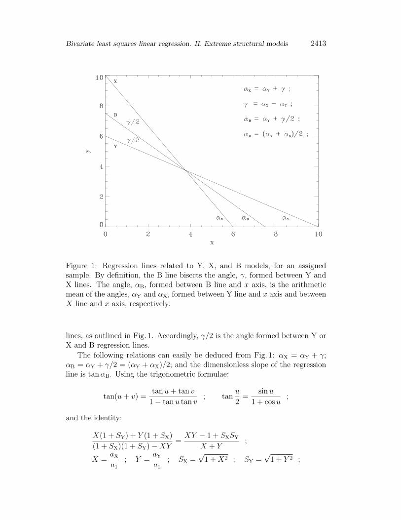
2.7 Bisector regression

The bisector regression implies use of both Y and X models for determiningthe angle formed by related regression lines. The bisecting line is assumed tobe the estimated regression line of the model.

Let αY, αX, αB, be the angles formed between Y, X, B, regression line,respectively, and x axis, and γ the angle formed between Y and X regression


Figure 1: Regression lines related to Y, X, and B models, for an assignedsample. By definition, the B line bisects the angle, γ, formed between Y andX lines. The angle, αB, formed between B line and x axis, is the arithmeticmean of the angles, αY and αX, formed between Y line and x axis and betweenX line and x axis, respectively.

lines, as outlined in Fig. 1. Accordingly, γ/2 is the angle formed between Y orX and B regression lines.

The following relations can easily be deduced from Fig. 1: αX = αY + γ;αB = αY + γ/2 = (αY + αX)/2; and the dimensionless slope of the regressionline is tanαB. Using the trigonometric formulae:

tan(u+ v) =tanu+ tan v

1− tanu tan v; tan

u

2=

sinu

1 + cosu;

and the identity:

X(1 + SY) + Y (1 + SX)

(1 + SX)(1 + SY)−XY=XY − 1 + SXSY

X + Y;

X =aXa1

; Y =aYa1

; SX =√

1 +X2 ; SY =√

1 + Y 2 ;

2414 R. Caimmi

the regression line slope estimator, after some algebra, is expressed as [18]:

aB =aYaX − a21 +

√a21 + (aY)2

√a21 + (aX)2

aY + aX; (98)

where a1 is the unit slope, aY = S11/S20; aX = S02/S11; and the regression lineintercept estimator reads [18]:

bB = Y − aBX ; (99)

where the index, B, denotes bisector regression.The bisector regression may be considered as a special case of oblique

regression where the variance ratio, c2, is deduced from the combination ofEqs. (54) and (98), requiring aC = aB. After a lot of algebra involving theroots of a second-degree equation, the result is:

c2 = (aB)2aX ∓ aBaB

(aB ∓ aYaY

)−1; (100)

where the parasite solution must be disregarded. Accordingly, Eqs. (51) and(52) also hold.

For normal residuals and homoscedastic data, the regression line slope andintercept variance estimators may be directly inferred from Eqs. (56) and (57)in the limit, aC → aB. The result is:

[(σaB)N]2 =(aB)2

n− 2

[(n− 2)RB

aBS11

+ Θ(aB, aY, aX)

]

=(aB)2

n− 2

[aX − aBaB

+aB − aYaY

+ Θ(aB, aY, aX)

]; (101)

[(σbB)N]2 =[

1

aB

S11

S00

+ (X)2]

[(σaB)N]2 − aBn− 2

S11

S00

Θ(aB, aY, aX) ; (102)

and for non normal residuals the application of the δ-method yields [18]:

(σaB)2 =(aB)2

(aY + aX)2

[a21 + (aX)2

a21 + (aY)2(σaY)2 +

a21 + (aY)2

a21 + (aX)2(σaX)2 + 2σaYaX

]; (103)

(σbB)2 =aBn

[aX − aBaB

+aB − aYaY

]S11

S00

+ (X)2(σaB)2

− 2

nX(σbYaB

+ σbXaB) ; (104)

σbYaB=

aB√a21 + (aX)2

(aY + aX)√a21 + (aY)2

S12 + aYaBS30 − (aY + aB)S21

S20

; (105)

σbXaB=

aB√a21 + (aY)2

(aY + aX)√a21 + (aX)2

S03 + aXaBS21 − (aX + aB)S12

S11

; (106)


where σaYaX is defined by Eq. (60) and Eqs. (103), (104), are equivalent totheir counterparts expressed in the parent paper [18]. For further details, aninterested reader is addressed to Appendix D.

For heteroscedastic data, the combination of Eqs. (67) and (98), requiringaC = aB, after a lot of algebra involving the roots of a second-degree equation,yields:

c2 = (aB)2aX ∓ aBaB

(aB ∓ a′Ya′Y

)−1; (107)

where aX = (wx)02/(wx)11; a′Y = (wx)11/(wx)20; and the parasite solution must

be disregarded. Accordingly, Eqs. (51) and (52) also hold.The extension of the above results to heteroscedastic data via Eqs. (98)-(99)

and (101)-(106) reads:

bB = Y − aBX ; (108)

[(σaB)N]2 =(aB)2

n− 2

[n− 2

n

RB

aB

(wx)00(wx)11

+ Θ(aB, a′Y, aX)

]

=(aB)2

n− 2

[aX − aBaB

+aB − a′Ya′Y

+ Θ(aB, a′Y, aX)

]; (109)

[(σbB)N]2 =

[1

aB

(wx)11(wx)00

+ (X)2]

[(σaB)N]2 − aBn− 2

(wx)11(wx)00

Θ(aB, a′Y, aX); (110)

(σaB)2 =(aB)2

(aY + aX)2

[a21 + (aX)2

a21 + (aY)2(σaY)2 +

a21 + (aY)2


]; (111)

(σbB)2 =aBn

[aX − aBaB

+aB − a′Ya′Y

](wx)11(wx)00

+ (X)2(σa′B)2

− 2

nX(σbYaB

+ σbXaB) ; (112)

σbYaB=

aB√a21 + (aX)2

(aY + aX)√a21 + (aY)2

(wx)12 + aYaB(wx)30 − (aY + aB)(wx)21(wx)20

; (113)

σbXaB=

aB√a21 + (aY)2

(aY + aX)√a21 + (aX)2

(wx)03 + aXaB(wx)21 − (aX + aB)(wx)12(wx)11

; (114)

and, in addition:

(σa′B)2 =(aB)2

(aY + aX)2

[a21 + (aX)2

a21 + (aY)2(σa′Y)2 +

a21 + (aY)2


]; (115)

where aY = (wy)11/(wy)20; a′Y = (wx)11/(wx)20; aX = (wx)02/(wx)11; R is

defined in Appendix A, σaYaX , (σa′Y)2, are expressed by Eqs. (73), (80), respec-tively, and Θ is formulated in terms of n(wx)pq/(wx)00 instead of Spq.

2416 R. Caimmi


2.8 Extension to structural models

A nontrivial question is to what extent the above results, valid for extremestructural models, can be extended to typical structural models. In general,assumptions related to typical structural models are different from their coun-terparts related to extreme structural models e.g., [3] Chap. 6 §6.4.5 but, onthe other hand, they could coincide for a special subclass.

In any case, whatever different assumptions and models can be made withregard to typical and extreme structural models, results from the former areexpected to tend to their counterparts from the latter when the instrumentalscatter is negligible with respect to the intrinsic scatter. It is worth noticingthat most work on linear regression by astronomers involves the situation whereboth intrinsic scatter and heteroscedastic data are present e.g., [1] [27] [19] [20][17].

A special subclass of structural models with normal residuals can be definedwhere, for a selected regression estimator, the regression line slope and inter-cept variance estimators are independent of the amount of instrumental andintrinsic scatter, including the limit of null intrinsic scatter (functional models)and null instrumental scatter (extreme structural models). More specifically,the dependence occurs only via the total (instrumental + intrinsic) scatter. Inthis view, the whole subclass of structural models under consideration couldbe related to functional modelling [7] Chap. 2 §2.1. For further details, aninterested reader is addressed to the parent paper [6].

3 An example of astronomical application

3.1 Astronomical introduction

Heavy elements are synthesised within stars and (partially or totally) re-turned to the interstellar medium via supernovae. In an ideal situation wherethe initial stellar mass function (including binary and multiple systems) is uni-versal and the gas returned after star death is instantaneously and uniformlymixed with the interstellar medium, the abundance ratio of primary elementsproduced mainly by large-mass (m

>∼ 8m, where m is the solar mass) starsmaintains unchanged, which implies a linear relation. This is why large-massstars have a short lifetime with respect to the age of the universe, and re-lated ejecta (due to type II supernovae) may be considered as instantaneouslyreturned to the interstellar medium.


A linear relation also holds if low-mass (m<∼ 8m) stars are considered,

where the stellar lifetime can no longer be neglected with respect to the ageof the universe. Close binary systems including a white dwarf with masses,mWD + mC > mCh, are (type Ia) supernovae progenitors, where mWD is thewhite dwarf mass, mC is the companion mass, and mCh ≈ 1.44m is the Chan-drasekhar upper mass limit for stable white dwarfs. An additional restriction,for a linear relation between two generic primary elements in the interstellarmedium, is a constant number ratio of type II to type Ia supernovae at anyepoch. For further details, an interested reader is addressed to Appendix F.

Restricting to iron and oxygen, the generic linear relation, Eq. (227), reads:

[O/H]∗ = a[Fe/H]∗ + b ; (116)

where [O/H], [Fe/H], are logarithmic number abundances normalized to thesolar value e.g., [4] and the asterisks denote the ideal situation. More specifi-cally, oxygen and iron abundance determinations performed on ideal stars byuse of ideal instruments yield coordinates of points lying on the straight linedefined by Eq. (116).

The intrinsic dispersion outside or along the ideal regression line may beowing to several processes, such as fluctuations in the stellar initial mass func-tion (including binary and multiple systems) and inhomogeneous mixing ofstellar ejecta with the interstellar medium, at different rates for different ele-ments. Accordingly, ideal points, P∗i ≡ ([Fe/H]∗i , [O/H]∗i ), are shifted towardsactual points, PSi ≡ ([Fe/H]Si, [O/H]Si).

More specifically, coeval ideal stars are represented by a single point on theideal regression line, while related actual stars correspond to points which, ingeneral, are shifted to a different extent outside or along the ideal regressionline. Conversely, stars with different age could be represented by a same actualpoint, PSi. The occurrence of instrumental scatter, related to iron and oxygenabundance determination on a star sample, makes actual points, PSi, be shiftedtowards observed points, Pi ≡ ([Fe/H]i, [O/H]i).

With regard to the ideal regression line, there is a one-to-one correspon-dence between the coordinates, [Fe/H] and [O/H], while the contrary holdsfor actual points and observed points. In the limit of extreme structural mod-els, where instrumental scatter is negligible with respect to intrinsic scatter,observed points are very close to actual points (if otherwise, any linear depen-dence would be hidden). The latter, to a first extent, may be determined alongthe following steps.

(1) Estimate a plausible regression line.

(2) Calculate the mean distance of observed points from the estimated regres-sion line, parallel to each coordinate axis.

2418 R. Caimmi

(3) Subdivide each coordinate axis into bins of width equal to the relatedmean distance calculated in (2).

(4) Evaluate the intrinsic scatter within each bin, using the method describedin an earlier attempt [1].

(5) Minimize the loss function and determine the regression line slope andintercept estimators.

(6) Verify the absolute difference between previous and current regression lineslope and intercept estimators is less than a previously assigned tolerancevalue. If otherwise, return to (2) taking into consideration the currentestimated regression line.

In general, the total scatter, σ2[W/H]i

= σ2[W/H]Fi

+ σ2[W/H]Si

, should be used forevaluating the weights, wxi

, wyi , 1 ≤ i ≤ n, appearing in the sum of thesquared residuals, expressed by Eq. (8a), which implies the knowledge of theinstrumental covariance matrix e.g., [1] [20].

3.2 Statistical results

An astronomical application performed in an earlier attempt [6] with re-gard to functional models, shall be repeated here for extreme structural models.Accordingly, related samples will be left unchanged but with the additional as-sumptions: (i) the intrinsic scatter is dominant with respect to the instrumen-tal scatter, and (ii) uncertainties mentioned in the parent papers and reportedbelow are related to the intrinsic scatter.

More specifically, the following samples related to the [O/H]-[Fe/H] relationshall be considered: RB09 [25], n = 49, heteroscedastic data; Fa09 [10], n = 44,homoscedastic data with three different [O/H] determinations, namely LTE(standard local thermodynamical equilibrium for one-dimensional hydrostaticmodel atmospheres), SH0 (three-dimensional hydrostatic model atmospheresin absence of LTE with no account taken of the inelastic collisions via neutralH atoms, SH = 0), SH1 (three-dimensional hydrostatic model atmospheres inabsence of LTE with due account taken of the inelastic collisions via neutral Hatoms, SH = 1); Sa09 [26], n = 63, heteroscedastic data. For further details,an interested reader is addressed to the parent paper [5]. In any case, [Fe/H]and [O/H] are determined independently for each sample star.

The [O/H]-[Fe/H] empirical relations are interpolated using the regressionmodels, G, Y, X, O, R, B, for heteroscedastic data (FB09 and Sa09 samples)and Y, X, O, R, B, for homoscedastic data (Fa09 sample, cases LTE, SH0, SH1)and heteroscedastic data where intrinsic scatters are taken equal to the typicaluncertainties mentioned in the parent papers (FB09, Sa09), σ[Fe/H] = 0.15,σ[O/H] = 0.15, for both FB09 and Sa09 samples. Model G relates to a general


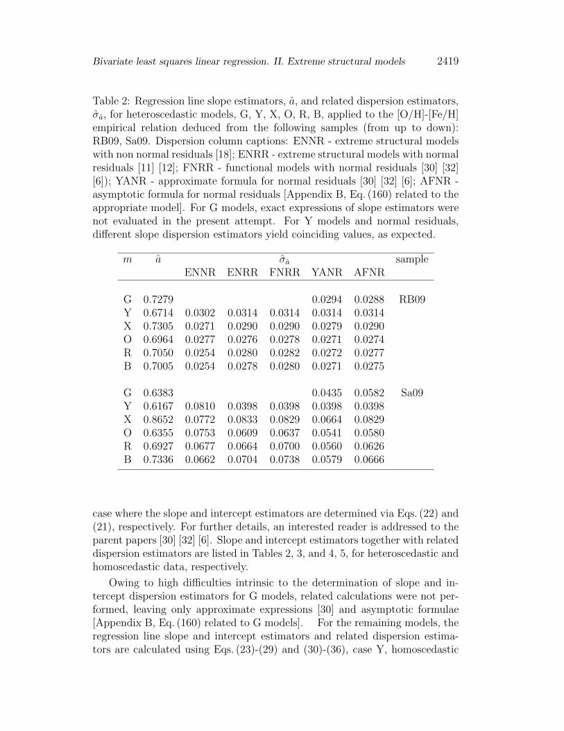
Table 2: Regression line slope estimators, a, and related dispersion estimators,σa, for heteroscedastic models, G, Y, X, O, R, B, applied to the [O/H]-[Fe/H]empirical relation deduced from the following samples (from up to down):RB09, Sa09. Dispersion column captions: ENNR - extreme structural modelswith non normal residuals [18]; ENRR - extreme structural models with normalresiduals [11] [12]; FNRR - functional models with normal residuals [30] [32][6]); YANR - approximate formula for normal residuals [30] [32] [6]; AFNR -asymptotic formula for normal residuals [Appendix B, Eq. (160) related to theappropriate model]. For G models, exact expressions of slope estimators werenot evaluated in the present attempt. For Y models and normal residuals,different slope dispersion estimators yield coinciding values, as expected.

m a σa sampleENNR ENRR FNRR YANR AFNR

G 0.7279 0.0294 0.0288 RB09Y 0.6714 0.0302 0.0314 0.0314 0.0314 0.0314X 0.7305 0.0271 0.0290 0.0290 0.0279 0.0290O 0.6964 0.0277 0.0276 0.0278 0.0271 0.0274R 0.7050 0.0254 0.0280 0.0282 0.0272 0.0277B 0.7005 0.0254 0.0278 0.0280 0.0271 0.0275

G 0.6383 0.0435 0.0582 Sa09Y 0.6167 0.0810 0.0398 0.0398 0.0398 0.0398X 0.8652 0.0772 0.0833 0.0829 0.0664 0.0829O 0.6355 0.0753 0.0609 0.0637 0.0541 0.0580R 0.6927 0.0677 0.0664 0.0700 0.0560 0.0626B 0.7336 0.0662 0.0704 0.0738 0.0579 0.0666

case where the slope and intercept estimators are determined via Eqs. (22) and(21), respectively. For further details, an interested reader is addressed to theparent papers [30] [32] [6]. Slope and intercept estimators together with relateddispersion estimators are listed in Tables 2, 3, and 4, 5, for heteroscedastic andhomoscedastic data, respectively.

Owing to high difficulties intrinsic to the determination of slope and in-tercept dispersion estimators for G models, related calculations were not per-formed, leaving only approximate expressions [30] and asymptotic formulae[Appendix B, Eq. (160) related to G models]. For the remaining models, theregression line slope and intercept estimators and related dispersion estima-tors are calculated using Eqs. (23)-(29) and (30)-(36), case Y, homoscedastic

2420 R. Caimmi

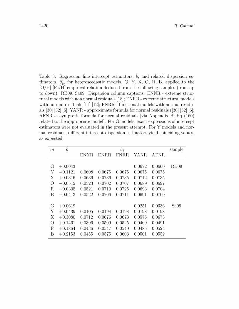
Table 3: Regression line intercept estimators, b, and related dispersion es-timators, σb, for heteroscedastic models, G, Y, X, O, R, B, applied to the[O/H]-[Fe/H] empirical relation deduced from the following samples (from upto down): RB09, Sa09. Dispersion column captions: ENNR - extreme struc-tural models with non normal residuals [18]; ENRR - extreme structural modelswith normal residuals [11] [12]; FNRR - functional models with normal residu-als [30] [32] [6]; YANR - approximate formula for normal residuals ([30] [32] [6];AFNR - asymptotic formula for normal residuals [via Appendix B, Eq. (160)related to the appropriate model]. For G models, exact expressions of interceptestimators were not evaluated in the present attempt. For Y models and nor-mal residuals, different intercept dispersion estimators yield coinciding values,as expected.

m b σb sampleENNR ENRR FNRR YANR AFNR

G +0.0043 0.0672 0.0660 RB09Y −0.1121 0.0608 0.0675 0.0675 0.0675 0.0675X +0.0316 0.0636 0.0736 0.0735 0.0712 0.0735O −0.0512 0.0523 0.0702 0.0707 0.0689 0.0697R −0.0305 0.0521 0.0710 0.0725 0.0693 0.0704B −0.0413 0.0522 0.0706 0.0711 0.0691 0.0700

G +0.0619 0.0251 0.0336 Sa09Y +0.0439 0.0105 0.0198 0.0198 0.0198 0.0198X +0.3080 0.0712 0.0676 0.0673 0.0575 0.0673O +0.1461 0.0396 0.0509 0.0525 0.0469 0.0491R +0.1864 0.0436 0.0547 0.0549 0.0485 0.0524B +0.2153 0.0455 0.0575 0.0603 0.0501 0.0552


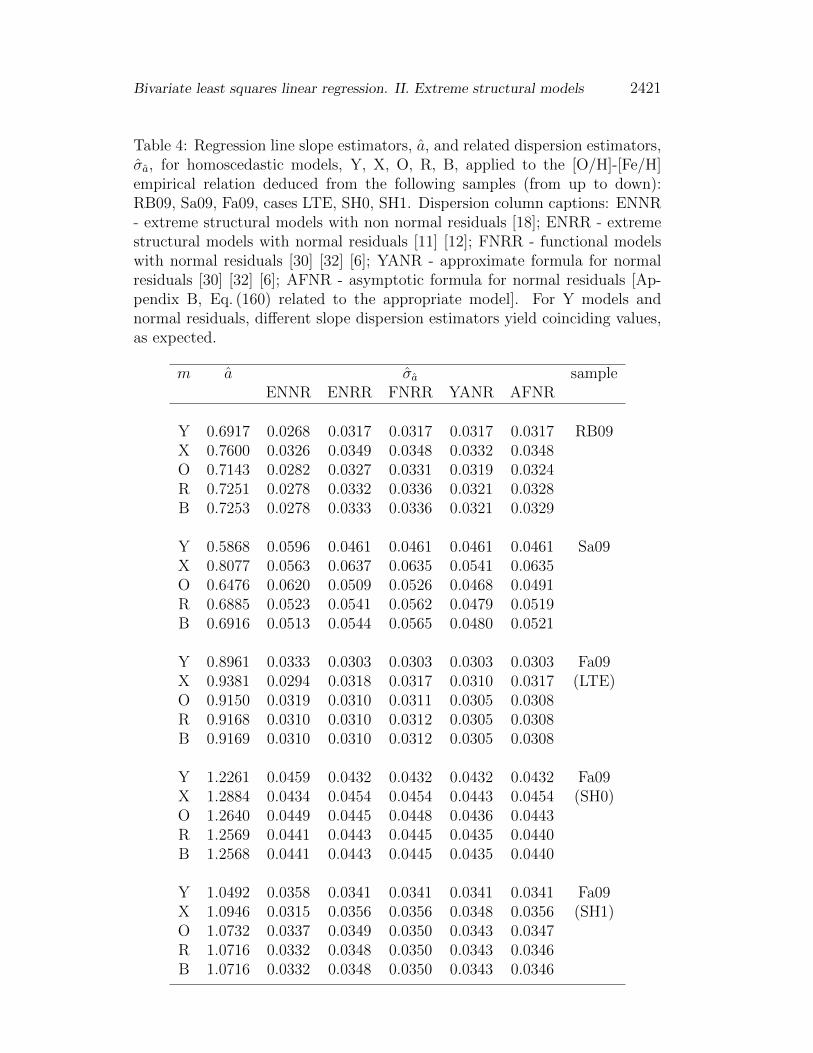
Table 4: Regression line slope estimators, a, and related dispersion estimators,σa, for homoscedastic models, Y, X, O, R, B, applied to the [O/H]-[Fe/H]empirical relation deduced from the following samples (from up to down):RB09, Sa09, Fa09, cases LTE, SH0, SH1. Dispersion column captions: ENNR- extreme structural models with non normal residuals [18]; ENRR - extremestructural models with normal residuals [11] [12]; FNRR - functional modelswith normal residuals [30] [32] [6]; YANR - approximate formula for normalresiduals [30] [32] [6]; AFNR - asymptotic formula for normal residuals [Ap-pendix B, Eq. (160) related to the appropriate model]. For Y models andnormal residuals, different slope dispersion estimators yield coinciding values,as expected.

m a σa sampleENNR ENRR FNRR YANR AFNR

Y 0.6917 0.0268 0.0317 0.0317 0.0317 0.0317 RB09X 0.7600 0.0326 0.0349 0.0348 0.0332 0.0348O 0.7143 0.0282 0.0327 0.0331 0.0319 0.0324R 0.7251 0.0278 0.0332 0.0336 0.0321 0.0328B 0.7253 0.0278 0.0333 0.0336 0.0321 0.0329

Y 0.5868 0.0596 0.0461 0.0461 0.0461 0.0461 Sa09X 0.8077 0.0563 0.0637 0.0635 0.0541 0.0635O 0.6476 0.0620 0.0509 0.0526 0.0468 0.0491R 0.6885 0.0523 0.0541 0.0562 0.0479 0.0519B 0.6916 0.0513 0.0544 0.0565 0.0480 0.0521

Y 0.8961 0.0333 0.0303 0.0303 0.0303 0.0303 Fa09X 0.9381 0.0294 0.0318 0.0317 0.0310 0.0317 (LTE)O 0.9150 0.0319 0.0310 0.0311 0.0305 0.0308R 0.9168 0.0310 0.0310 0.0312 0.0305 0.0308B 0.9169 0.0310 0.0310 0.0312 0.0305 0.0308

Y 1.2261 0.0459 0.0432 0.0432 0.0432 0.0432 Fa09X 1.2884 0.0434 0.0454 0.0454 0.0443 0.0454 (SH0)O 1.2640 0.0449 0.0445 0.0448 0.0436 0.0443R 1.2569 0.0441 0.0443 0.0445 0.0435 0.0440B 1.2568 0.0441 0.0443 0.0445 0.0435 0.0440

Y 1.0492 0.0358 0.0341 0.0341 0.0341 0.0341 Fa09X 1.0946 0.0315 0.0356 0.0356 0.0348 0.0356 (SH1)O 1.0732 0.0337 0.0349 0.0350 0.0343 0.0347R 1.0716 0.0332 0.0348 0.0350 0.0343 0.0346B 1.0716 0.0332 0.0348 0.0350 0.0343 0.0346

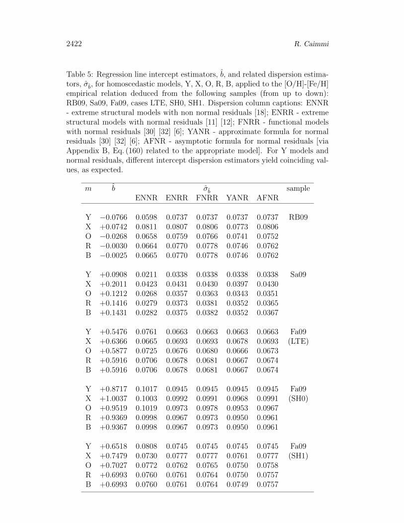
2422 R. Caimmi

Table 5: Regression line intercept estimators, b, and related dispersion estima-tors, σb, for homoscedastic models, Y, X, O, R, B, applied to the [O/H]-[Fe/H]empirical relation deduced from the following samples (from up to down):RB09, Sa09, Fa09, cases LTE, SH0, SH1. Dispersion column captions: ENNR- extreme structural models with non normal residuals [18]; ENRR - extremestructural models with normal residuals [11] [12]; FNRR - functional modelswith normal residuals [30] [32] [6]; YANR - approximate formula for normalresiduals [30] [32] [6]; AFNR - asymptotic formula for normal residuals [viaAppendix B, Eq. (160) related to the appropriate model]. For Y models andnormal residuals, different intercept dispersion estimators yield coinciding val-ues, as expected.

m b σb sampleENNR ENRR FNRR YANR AFNR

Y −0.0766 0.0598 0.0737 0.0737 0.0737 0.0737 RB09X +0.0742 0.0811 0.0807 0.0806 0.0773 0.0806O −0.0268 0.0658 0.0759 0.0766 0.0741 0.0752R −0.0030 0.0664 0.0770 0.0778 0.0746 0.0762B −0.0025 0.0665 0.0770 0.0778 0.0746 0.0762

Y +0.0908 0.0211 0.0338 0.0338 0.0338 0.0338 Sa09X +0.2011 0.0423 0.0431 0.0430 0.0397 0.0430O +0.1212 0.0268 0.0357 0.0363 0.0343 0.0351R +0.1416 0.0279 0.0373 0.0381 0.0352 0.0365B +0.1431 0.0282 0.0375 0.0382 0.0352 0.0367

Y +0.5476 0.0761 0.0663 0.0663 0.0663 0.0663 Fa09X +0.6366 0.0665 0.0693 0.0693 0.0678 0.0693 (LTE)O +0.5877 0.0725 0.0676 0.0680 0.0666 0.0673R +0.5916 0.0706 0.0678 0.0681 0.0667 0.0674B +0.5916 0.0706 0.0678 0.0681 0.0667 0.0674

Y +0.8717 0.1017 0.0945 0.0945 0.0945 0.0945 Fa09X +1.0037 0.1003 0.0992 0.0991 0.0968 0.0991 (SH0)O +0.9519 0.1019 0.0973 0.0978 0.0953 0.0967R +0.9369 0.0998 0.0967 0.0973 0.0950 0.0961B +0.9367 0.0998 0.0967 0.0973 0.0950 0.0961

Y +0.6518 0.0808 0.0745 0.0745 0.0745 0.0745 Fa09X +0.7479 0.0730 0.0777 0.0777 0.0761 0.0777 (SH1)O +0.7027 0.0772 0.0762 0.0765 0.0750 0.0758R +0.6993 0.0760 0.0761 0.0764 0.0750 0.0757B +0.6993 0.0760 0.0761 0.0764 0.0749 0.0757


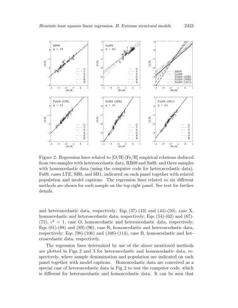
Figure 2: Regression lines related to [O/H]-[Fe/H] empirical relations deducedfrom two samples with heteroscedastic data, RB09 and Sa09, and three sampleswith homoscedastic data (using the computer code for heteroscedastic data),Fa09, cases LTE, SH0, and SH1, indicated on each panel together with relatedpopulation and model captions. The regression lines related to six differentmethods are shown for each sample on the top right panel. See text for furtherdetails.

and heteroscedastic data, respectively; Eqs. (37)-(43) and (44)-(50), case X,homoscedastic and heteroscedastic data, respectively; Eqs. (54)-(62) and (67)-(75), c2 = 1, case O, homoscedastic and heteroscedastic data, respectively;Eqs. (81)-(88) and (89)-(96), case R, homoscedastic and heteroscedastic data,respectively; Eqs. (98)-(106) and (108)-(114), case B, homoscedastic and het-eroscedastic data, respectively.

The regression lines determined by use of the above mentioned methodsare plotted in Figs. 2 and 3 for heteroscedastic and homoscedastic data, re-spectively, where sample denomination and population are indicated on eachpanel together with model captions. Homoscedastic data are conceived as aspecial case of heteroscedastic data in Fig. 2 to test the computer code, whichis different for heteroscedastic and homoscedastic data. It can be seen that

2424 R. Caimmi

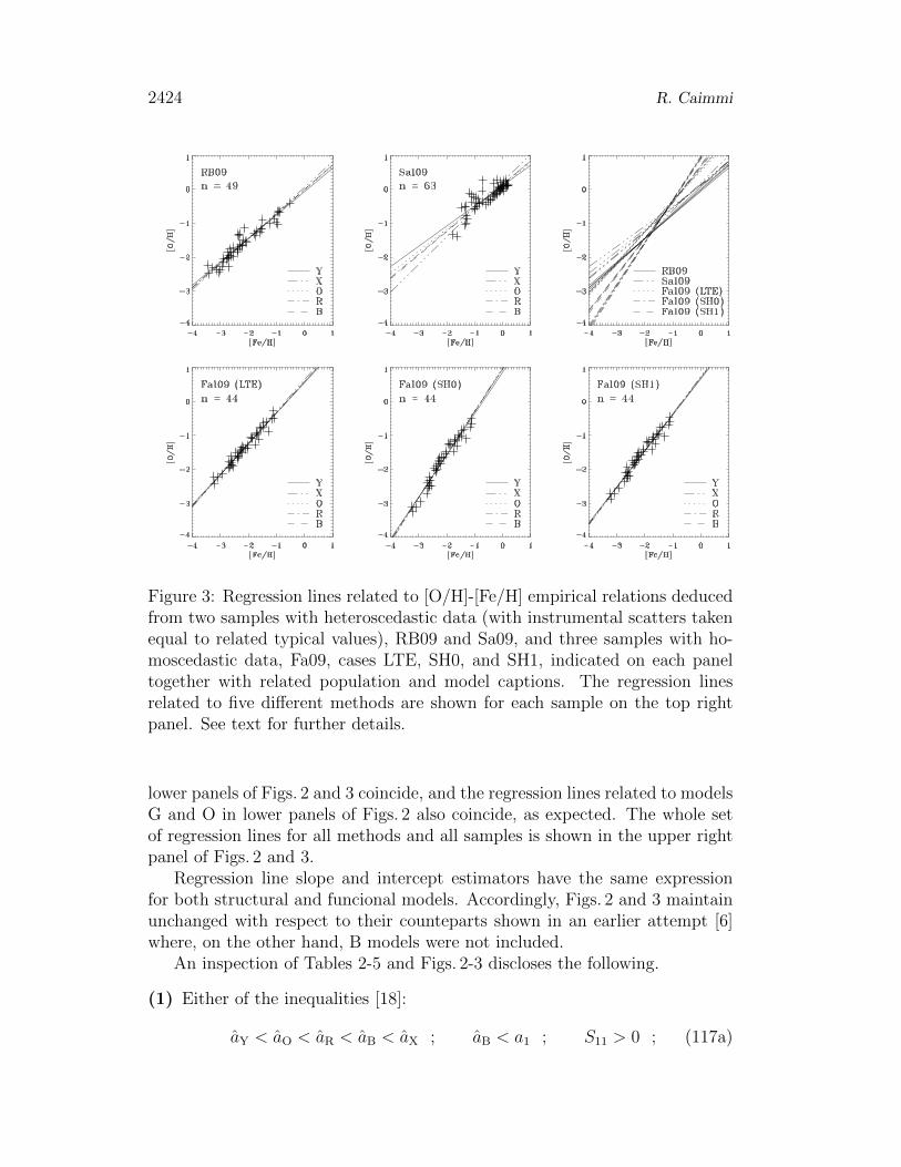
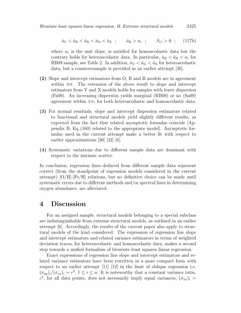
Figure 3: Regression lines related to [O/H]-[Fe/H] empirical relations deducedfrom two samples with heteroscedastic data (with instrumental scatters takenequal to related typical values), RB09 and Sa09, and three samples with ho-moscedastic data, Fa09, cases LTE, SH0, and SH1, indicated on each paneltogether with related population and model captions. The regression linesrelated to five different methods are shown for each sample on the top rightpanel. See text for further details.

lower panels of Figs. 2 and 3 coincide, and the regression lines related to modelsG and O in lower panels of Figs. 2 also coincide, as expected. The whole setof regression lines for all methods and all samples is shown in the upper rightpanel of Figs. 2 and 3.

Regression line slope and intercept estimators have the same expressionfor both structural and funcional models. Accordingly, Figs. 2 and 3 maintainunchanged with respect to their counteparts shown in an earlier attempt [6]where, on the other hand, B models were not included.

An inspection of Tables 2-5 and Figs. 2-3 discloses the following.

(1) Either of the inequalities [18]:

aY < aO < aR < aB < aX ; aB < a1 ; S11 > 0 ; (117a)


aY < aB < aR < aO < aX ; aB > a1 ; S11 > 0 ; (117b)

where a1 is the unit slope, is satisfied for homoscedastic data but thecontrary holds for heteroscedastic data. In particular, aB < aR < a1 forRB09 sample, see Table 2. In addition, aY < aG < aX for heteroscedasticdata, but a counterexample is provided in an earlier attempt [30].

(2) Slope and intercept estimators from O, R and B models are in agreementwithin ∓σ. The extension of the above result to slope and interceptestimators from Y and X models holds for samples with lower dispersion(Fa09). An increasing dispersion yields marginal (RB09) or no (Sa09)agreement within ∓σ, for both heteroscedastic and homoscedastic data.

(3) For normal residuals, slope and intercept dispersion estimators relatedto functional and structural models yield slightly different results, asexpected from the fact that related asymptotic formulae coincide [Ap-pendix B, Eq. (160) related to the appropriate model]. Asymptotic for-mulae used in the current attempt make a better fit with respect toearlier approximations [30] [32] [6].

(4) Systematic variations due to different sample data are dominant withrespect to the intrinsic scatter.

In conclusion, regression lines deduced from different sample data representcorrect (from the standpoint of regression models considered in the currentattempt) [O/H]-[Fe/H] relations, but no definitive choice can be made untilsystematic errors due to different methods and/or spectral lines in determiningoxygen abundance, are alleviated.

4 Discussion

For an assigned sample, structural models belonging to a special subclassare indistinguishable from extreme structural models, as outlined in an earlierattempt [6]. Accordingly, the results of the current paper also apply to struc-tural models of the kind considered. The expression of regression line slopeand intercept estimators and related variance estimators in terms of weighteddeviation traces, for heteroscedastic and homoscedastic data, makes a secondstep towards a unified formalism of bivariate least squares linear regression.

Exact expressions of regression line slope and intercept estimators and re-lated variance estimators have been rewritten in a more compact form withrespect to an earlier attempt [11] [12] in the limit of oblique regression i.e.(σyy)i/(σxx)i = c2, 1 ≤ i ≤ n. It is noteworthy that a constant variance ratio,c2, for all data points, does not necessarily imply equal variances, (σxx)i =

2426 R. Caimmi

σxx = const, (σyy)i = σyy = const, 1 ≤ i ≤ n. While regression line slope andintercept estimators attain a coinciding expression in different attempts [30][32] [18] [11] [12], the results of the current paper show that the contrary holdsfor related variance estimators. The same holds for both reduced major-axisand bisector regression.

Approximate expressions provided in earlier attempts for normal residuals[30] [32] make (at least in computed cases) a lower limit to their exact counter-parts, as shown in Tables 2-5, YANR vs. ENRR, FNRR. The same holds, to abetter extent, for the asymptotic expressions determined in the current paper,as shown in Tables 2-5, AFNR vs. ENRR, FNRR. Related fractional discrep-ancies for low-dispersion data (RB09, Fa09) do not exceed a few percent, whichgrows up to about 10% in presence of large-dispersion data (Sa09).

It is well known that the regression line slope and intercept estimators arebiased towards zero for Y models e.g., [14] Chap. 1 §1.1.1 [7] Chap. 3 §3.2 [19][20] [3] Chap. 4 §4.4. Biases can be explicitly expressed in the special case ofhomoscedastic models with normal residuals. More specifically, the condition1−ρ20 1 ensures bias effects are negligible, where ρ20 is the reliability ratio:

ρ20 =S20

S20 + (n− 1)σxx; (118)

which implies 0 ≤ ρ20 ≤ 1. For further details, an interested reader is addressedto specific monographies e.g., [14] Chap. 1 §1.1.1 [7] Chap. 3 §3.2.1 [3] Chap. 4§4.4.

Similarly, it can be seen that regression line slope and intercept varianceestimators are biased towards infinity for X models. In the special case ofhomoscedastic models with normal residuals, the condition 1−ρ02 1 ensuresbias effects are negligible, where ρ02 is the reliability ratio:

ρ02 =S02

S02 + (n− 1)σyy; (119)

which implies 0 ≤ ρ02 ≤ 1 e.g., [6].

Accordingly, slopes are understimated in Y models and overstimated in Xmodels by a factor, ρ20 and 1/ρ02, respectively. For C models (oblique re-gression), O models (orthogonal regression), R models (reduced major-axisregression), B models (bisector regression), the regression line slope estima-tors lie between their counterparts related to Y and X models, according toEqs. (118) and (119), which implies bias corrections e.g., [7] Chap. 3 §3.4.2.Though there is skepticism about an indiscriminate use of oblique regressionestimators, still it is accepted the method is viable provided both instrumentaland intrinsic covariance matrix are known e.g., [7] Chap. 3 §3.4.2 [3] Chap. 4§4.5.


With regard to heteroscedastic data, an inspection of Tables 2-5 shows thatfor lower dispersion data (RB09 sample) the values of regression line slope andintercept estimators, deduced for weighted (Tables 2-3) and unweighted (Ta-bles 4-5) data, are systematically smaller in the former case with respect to thelatter, but are still in agreement within ∓σ. For larger dispersion data (Sa09sample) no systematic trend of the kind considered appears, but the valuesof regression line slope and intercept estimators are still in agreement within∓σ for O, R, and B models. It may be a general property of the regressionmodels considered in the current attempt or, more realistically, intrinsic to thesamples selected for the application performed in subsection 3.2.

The reliability ratios, Eqs. (118) and (119), have been calculated for allsample data and the inequalities, ρ20 > 0.92, ρ02 > 0.91, hold in any caseexcept ρ02 > 0.86 for the Sa09 sample, which implies poorly biased regressionline slope and intercept estimators for the samples considered using Y and Xmodels and, a fortiori, using C, O, R, and B models.

Numerical simulations can determine the performance of the regressioncoefficients in presence of small samples and large scatter, and evaluate whetherthe approximations made in deriving variances are accurate. According to theresults of a classical paper [18], the uncertainties to the slope predicted by Omodels are, on average, larger than those predicted by Y, R, or B models.For this reason, skepticism is expressed towards O models and, in any case,caution is urged in interpreting slopes when small samples and large scatterare involved [18].

On the other hand, O models are special cases of C models, which couldalso include R and B models, and the predicted slopes lie between their coun-terparts related to the limiting cases of Y and X models. Extended numericalsimulations should be used for searching a relation between the family of Cmodels, c2 = c2min, with the lowest uncertainty to the slope, and values of pop-ulation variances and covariance, namely c2min = f(σXX , σY Y , σXY ). In thisview, it should be recommended use of C models where c2 = c2min for assignedsample variances and covariance, which estimate their counterparts related tothe parent population.

Concerning samples listed in Tables 2-5 and represented in Figs. 2-3, theslope uncertainty predicted by O models is slightly larger than the slope pre-dicted by R and B models for non normal residuals (ENNR), while the reverseoccurs for normal residuals (ENNR). In addition, the slope uncertainty pre-dicted by G models (the general case), when estimated, is close to the slopeuncertainty predicted by O, R, and B models.

5 Conclusion

From the standpoint of a unified analytic formalism of bivariate least

2428 R. Caimmi

squares linear regression, extreme structural models have been conceived asa limiting case where the instrumental scatter is negligible (ideally null) withrespect to the intrinsic scatter.

Within the framework of a variant of the classical additive error modele.g., [7] Chap. 1 §1.2, Chap. 3 §3.2.1 [3] Chap. 4 §4.3 [20], the classical resultspresented in earlier papers [18] [11] [12] have been rewritten in a more compactform using a new formalism in terms of weighted deviation traces which, forhomoscedastic data, reduce to usual quantities, leaving aside an unessential(but dimensional) multiplicative factor.

Regression line slope and intercept estimators, and related variance estima-tors, have been expressed in the special case of uncorrelated errors in X andin Y for the following models: (Y) errors in X negligible (ideally null) withrespect to errors in Y ; (X) errors in Y negligible (ideally null) with respectto errors in X; (C) oblique regression; (O) orthogonal regression; (R) reducedmajor-axis regression; (B) bisector regression. Related variance estimatorshave been expressed for both non normal and normal residuals and comparedto their counterparts determined for functional models [6] [32].

Under the assumption that regression line slope and intercept variance es-timators for homoscedastic and heteroscedastic data are connected to a similarextent in functional and structural models, the above mentioned results havebeen extended from homoscedastic to heteroscedastic data. In absence of arigorous proof, related expressions have been considered as approximate re-sults.

An example of astronomical application has been considered, concerningthe [O/H]-[Fe/H] empirical relations deduced from five samples related to dif-ferent populations and/or different methods of oxygen abundance determina-tion. For low-dispersion samples and assigned methods, different regressionmodels have been found to yield results which are in agreement within the er-rors (∓σ) for both heteroscedastic and homoscedastic data, while the contraryhas been shown to hold for large-dispersion samples. In any case, samplesrelated to different methods have been found to produce discrepant results,due to the presence of (still undetected) systematic errors, which implies nodefinitive statement can be made at present.

Asymptotic expressions have been found to approximate regression lineslope and intercept variance estimators, for normal residuals, to a better extentwith respect to earlier attempts [30] [32]. Related fractional discrepancies havebeen shown to be not exceeding a few percent for low-dispersion data, whichhas grown up to about 10% in presence of large-dispersion data.

An extension of the formalism to generic structural models has been leftto future work.

Acknowledgements. Thanks are due to G.J. Babu, E.D. Feigelson, M.A.


Bershady, I. Lavagnini, S.J. Schmidt, for fruitful e-mail correspondance ontheir quoted papers [11] [12] [1] [22] [26] respectively. The author is indebtedto G.J. Babu and E.D. Feigelson for having kindly provided the erratum oftheir quoted paper [11] before publication [12].

References

[1] M.G. Akritas, M.A. Bershady, Linear Regression for Astronomical Datawith Measurement Errors and Intrinsic Scatter, The Astrophysical Journal,470 (1996), 706-714. https://doi.org/10.1086/177901

[2] P.J. Brown, Mesaurement, Regression and Calibration, Oxford StatisticalScience Series 12, Oxford Science Publications, Oxford, 1993.

[3] J.P. Buonaccorsi, Mesaurement Error: Models, Methods and Applications,Chapman & Hall/CRC, London, 2010.https://doi.org/10.1201/9781420066586

[4] R. Caimmi, The G-dwarf problem in the Galactic spheroid, New Astron-omy, 12 (2007), 289-321. https://doi.org/10.1016/j.newast.2006.10.007

[5] R. Caimmi, A Simple Multistage Closed-(Box+Reservoir) Model of Chem-ical Evolution, Serbian Astronomical Journal, 183 (2011), 37-61.https://doi.org/10.2298/saj1183037c

[6] R. Caimmi, Bivariate least squares linear regression: Towards a unifiedanalytic formalism. I. Functional models, New Astronomy, 16 (2011), 337-356. https://doi.org/10.1016/j.newast.2011.01.001

[7] R.J. Carroll, T.D. Ruppert, L.A. Stefanski, C.M. Crainiceanu, Mesaure-ment Error in Nonlinear Models, Monographs on Statistics and AppliedProbability 105, Chapman & Hall/CRC, London, 2006.https://doi.org/10.1201/9781420010138

[8] A. Cuevas, A partial overview of the theory of statistics with functionaldata, Journal of Statistical Planning and Inference, 147 (2014), 1-23.https://doi.org/10.1016/j.jspi.2013.04.002

[9] A. Delaigle, P. Hall, Classification using censored functional data, Journalof the American Statistical Association, 108 (2013), 1269-1283.https://doi.org/10.1080/01621459.2013.824893

[10] D. Fabbian, P.E. Nissen, M. Asplund, M. Pettini, C. Akerman, The C/Oratio at low metallicity: constraints on early chemical evolution from ob-servations of Galactic halo stars, Astronomy and Astrophysics, 500 (2009),1143-1155. https://doi.org/10.1051/0004-6361/200810095

2430 R. Caimmi

[11] E.D. Feigelson, G.J. Babu, Linear regression in astronomy. II, The Astro-physical Journal, 397 (1992), 55-67. https://doi.org/10.1086/171766

[12] E.D. Feigelson, G.J. Babu, ERRATUM: Linear Regression in Astronomy.II, The Astrophysical Journal, 728 (2011), 72-72.https://doi.org/10.1088/0004-637x/728/1/72

[13] E.D. Feigelson, G.J. Babu, G. Jogesh, Statistical Methods for Astronomy,Chapter in Planets, Stars and Stellar Systems, by T.D. Ostwalt, H.E. Bond,Springer Science+Business Media, Dordrecht, 2013, 445-480.https://doi.org/10.1007/978-94-007-5618-2 10

[14] W.A. Fuller, Mesaurement Error Models, J. Wiley & Sons, Hoboken, 1987.https://doi.org/10.1002/9780470316665

[15] J.S. Garden, D.G. Mitchell, W.N. Mills, Nonconstant Variance RegressionTechniques for Calibration-Curve-Based Analysis, Analytical Chemistry, 52(1980), 2310-2315. https://doi.org/10.1021/ac50064a017

[16] P. Hall, G. Hooker, Truncated Linear Models for Functional Data, Journalof the Royal Statistical Society, Series B, 78 (2016), 637-653.https://doi.org/10.1111/rssb.12125

[17] J.M. Hilbe, R.S. de Souza, E.E.O. Ishida, Bayesian Models for Astrophys-ical Data, Cambridge University Press, Cambridge, 2017.https://doi.org/10.1017/cbo9781316459515

[18] T. Isobe, E.D. Feigelson, M.G. Akritas, G.J. Babu, Linear regression inastronomy, The Astrophysical Journal, 364 (1990), 104-113.https://doi.org/10.1086/169390

[19] B.C. Kelly, Some Aspects of Measurement Error in Linear Regressionof Astronomical Data, The Astrophysical Journal, 665 (2007), 1489-1506.https://doi.org/10.1086/519947

[20] B.C. Kelly, Mesaurement Error Models in Astronomy, in Statistical Chal-lenges in Modern Astronomy V, E.D. Feigelson, G.J. Babu, (eds), SpringerScience+Business Media, New York, 147-162.https://doi.org/10.1007/978-1-4614-3520-4 13

[21] A. Kneip, D. Poss, P. Sarda, Functional linear regression with points ofimpact, The Annals of Statistics, 44 (2016), 1-30.https://doi.org/10.1214/15-aos1323


[22] I. Lavagnini, F. Magno, A statistical overview on univariate calibration,inverse regression, and detection limits: application to gas chromatogra-phy/mass spectrometry technique, Mass Spectrometry Reviews, 26 (2007),1-18. https://doi.org/10.1002/mas.20100

[23] R.P. Miller, Simultaneous Statistical Inference, McGrew-Hil, New York,1966.

[24] C. Osborne, Statistical calibration: a review, International Statistical Re-view, 59 (1991), 309-336. https://doi.org/10.2307/1403690

[25] J.A. Rich, A.M. Boesgaard, Beryllium, Oxygen, and Iron Abundances inExtremely Metal-Deficient Stars, The Astrophysical Journal, 701 (2009),1519-1533. https://doi.org/10.1088/0004-637x/701/2/1519

[26] S.J. Schmidt, G. Wallerstein, V.M. Woolf, J.L. Bean, Cool Star OxygenAbundances from Spectral Synthesis of TiO Bands, Publications of the As-tronomical Society of Pacific, 121 (2009), 1083-1089.https://doi.org/10.1086/644605

[27] S. Tremaine, K. Ghebhardt, R. Bender, G. Bower, A. Dressler, S.M.Faber, A.V. Filippenko, R. Green, C. Grillmair, L.C. Ho, J. Kormendy,T.R. Lauer, J. Magorrian, J. Pinkney, D. Richstone, The Slope of the BlackHole Mass versus Velocity Dispersion Correlation, The Astrophysical Jour-nal, 574 (2002), 740-753. https://doi.org/10.1086/341002

[28] X. Wang, D. Ruppert, Optimal Prediction in an Additive FunctionalModel, Statistica Sinica, 25 (2015), 567-589.https://doi.org/10.5705/ss.2013.074

[29] J.L. Wang, J.M. Chiou, H.G. Muller, Review of functional data analysis,Annual Review of Statistics and Its Application, 3 (2016), 257-295.

[30] D. York, Least-squares fitting of a straight line, Canadian Journal ofPhysics, 44 (1966), 1079-1086. https://doi.org/10.1139/p66-090

[31] D. York, The best isochron, Earth and Planetary Science Letters, 2 (1967),479-482. https://doi.org/10.1016/0012-821x(67)90193-8

[32] D. York, Least squares fitting of a straight line with correlated errors,Earth and Planetary Science Letters, 5 (1969), 320-324.https://doi.org/10.1016/s0012-821x(68)80059-7

2432 R. Caimmi

Appendix

A Euclidean and statistical squared residual

sum

For homoscedastic data, the sum of squared (dimensional) Euclidean dis-tances between observed points, Pi(Xi, Yi), and adjusted points on the esti-mated regression line, Pi(xi, yi), yi = axi + b, is expressed as e.g., [14] Chap. 1§1.3.3 [11] [12] [6]:

(n− 2)R =n∑

i=1

[(Yi − Y )− a(Xi −X)

]2= S02 + (a)2S20 − 2aS11 ; (120)

where R is denoted as svv in the earlier quotation [14].

The sum of squared (dimensionless) statistical distances e.g., [14] Chap. 1§1.3.3 between the above mentioned points, Pi(Xi, Yi) and Pi(xi, yi), reads [6]:

TR = W[S02 + (a)2S20 − 2aS11

]; (121)

which, for heteroscedastic data, takes the general expression [6]:

TR

= W02 + (a)2W20 − 2aW11 ; (122)

accordingly, the extension of Eq. (120) to heteroscedastic data reads:

(n− 2)R =n[W02 + (a)2W20 − 2aW11]

W00

; (123)

which, in the limit of homoscedastic data, Wi = W = W , 1 ≤ i ≤ n, W00 =nW = nW , Wpq = WSpq, via Eqs. (9), (10), reduces to Eq. (120), as expected.

B Equivalence between earlier and current for-

mulation

Let oblique regression models be taken into consideration under the follow-ing restrictive assumptions: (1) homoscedastic data; (2) uncorrelated errorsin Y and in X; (3) normal residuals. Accordingly, the regression line slopevariance estimator is expressed by Eq. (56) where the function, Θ(aC, aY, aX),may be different for different methods and/or models, as shown in Table 1.Aiming to a formal demonstration, some preliminary relations are needed.


In terms of dimensionless ratios, using Eqs. (23) and (37), Eq. (120) trans-lates into:

(n− 2)R

aS11

=aXa

+a

aY− 2 =

aX − aa

+a− aYaY

; (124)

where the following identities:

aX − aa

+a− aYaY

=aX − aYaY

− aX − aa

a− aYaY

; (125)

aX − aa

a− aYaY

=aX − aYaY

− aX − aa− a− aY

aY=aX − aaY

− aX − aa

; (126)

may easily be verified.In the case under discussion of oblique regression models, a = aC, the

following inequalities hold [18]:

aX ≥ aC ≥ aY ; S11 > 0 ; (127)

aX ≤ aC ≤ aY ; S11 < 0 ; (128)

which makes the left-hand side of Eq. (124) always positive provided S11 6= 0.Using the method of partial differentiation, the regression line slope vari-

ance estimator in the case under discussion is [6]:

(σaC)2 =(aC)2

n− 2

[2S02S20 − (S11)

2

(S11)2+ 2− S02 + (aC)2S20

aCS11

]; (129)

and the substitution of Eqs. (23) and (37) into (129), using (125) and (126)yields after some algebra:

(σaC)2 =(aC)2

n− 2

[aX − aCaC

+aC − aYaY

+ 2aX − aCaC

aC − aYaY

]; (130)

from which the following is inferred by comparison with Eq. (56):

Θ(aC, aY, aX) = 2aX − aCaC

aC − aYaY

; (131)

as listed in Table 1.Using the method of moments estimators, the elements of the sample co-

variance matrix are:

mXX =S20

n− 1; mY Y =

S02

n− 1; mXY = mY X =

S11

n− 1; (132)

which, in terms of the variance estimators, (σxx)S (intrinsic x error distribu-tion), (σxx)F (instrumantal x error distribution), (σyy)F (instrumental y error

2434 R. Caimmi

distribution) via c2F = (σyy)F/(σxx)F, and regression line slope estimator, aC,are expressed as:

mXX = (σxx)S + (σxx)F ; (133a)

mY Y = (aC)2(σxx)S + (cF)2(σxx)F ; (133b)

mXY = mY X = aC(σxx)S ; (133c)

for further details and specification of the model, an interested reader is ad-dressed to the parent paper [14] Chap. 1 §1.3.2.

The substitution of Eqs. (132) and (133) into (120) yields:

(n− 2)RC = (n− 1)[(aC)2 + (cF)2](σxx)F ; (134)

where the variance ratio, (cF)2, may explicitly be expressed using Eqs. (132)and (133). The result is:

(cF)2 =aC(S02 − aCS11)

aCS20 − S11

; (135)

which, using Eq. (120) and performing some algebra, takes the equivalent form:

(aC)2 + (cF)2 =aC(n− 2)RC

aCS20 − S11

; (136)

finally, the substitution of Eq. (136) into (134) yields:

(σxx)F =aCS20 − S11

(n− 1)aC; (137)

where the dependence on the variance ratio, (cF)2, has been eliminated.In the limit of large samples (n 1, ideally n→ +∞) where, in addition,

S11 6= 0, the regression line slope variance estimator is [14] Chap. 1 §1.3.2:

(σaC)2 =1

n− 1

1

[(σxx)S]2

[(σxx)S + (σxx)F]RC − (aC)2[(σxx)F]2

; (138)

and the substitution of Eqs. (124), (132), (133), (137), into (138) yields aftersome algebra:

(σaC)2 =(aC)2

n− 2

×

aX − aCaC

+aC − aYaY

+aX − aCaC

aC − aYaY

+1

n− 1

(aC − aYaY

)2 ; (139)


Θ(aC, aY, aX) =aX − aCaC

aC − aYaY

+1

n− 1

(aC − aYaY

)2

; (140)


as listed in Table 1.On the other hand, the regression line slope variance estimator reported in

an earlier attempt [11] [12] Eq. (4), reads:

(σaC)2 =(aC)2

n− 2

[(n− 2)RC

aCS11

+aC(S02 − aCS11)

(cS)2(n− 2)RC

aC(S11)2

−n− 2

n− 1

(aC)2

(S11)2

(S02 − aCS11

(cS)2

)2 ; (141)

where cS = c and the counterpart of Eq. (135) holds [6]:

c2 = c2S =aC(S02 − aCS11)

aCS20 − S11

; (142)

and the substitution of Eqs. (124), (142), into (141), after some algebra yieldsEq. (139). Then the regression line slope variance estimator, expressed byEq. (141), coincides with its counterpart deduced via the method of momentestimators, expressed by Eq. (139).

Using the method of least squares estimation, under the assumption thatthe entire instrumental covariance matrix is known, the regression line slopevariance estimator reads [14] Chap. 1 §1.3.3:

(σaC)2 =1

n− 1

1

(mXX)2

mXX σvv + (σxx)Fσvv − (σxv)

2

; (143)

σvv = (σyy)F + (aC)2(σxx)F − 2aC(σxy)F ; (144)

σxv = (σxy)F − aC(σxx)F ; (145)

where mXX is the maximum likelihood estimator for (σxx)S, mXX = (σxx)S.In the special case under consideration, (σyy)F = (cF)2(σxx)F, (σxy)F = 0,

Eqs. (143), (144), (145), reduce to:

(σaC)2 =1

n− 1

1

(mXX)2

[mXX + (σxx)F] σvv − (aC)2[(σxx)F]2

; (146)

σvv = [(aC)2 + (cF)2](σxx)F ; (147)

σxv = −aC(σxx)F ; (148)

if, in addition, least squares estimators are proportional to corresponding mo-ments estimators, the following relations hold:

[(σxx)U]lsc = CXU[(σxx)U]mme ; U = F, S ; (149a)

(σvv)lsc = Cv(σvv)mme ; (149b)

where CXU, Cv, are constants and the indices, lsc, mme, mean least squares

estimators and methods of moments estimators, respectively.

2436 R. Caimmi

The substitution of Eq. (149) into (146) yields:

(σaC)2 =1

n− 1

1

(CXS)2[(σxx)S]2

[CXS

(σxx)S + CXF(σxx)F]Cv[(aC)2 + (cF)2]

× (σxx)F − (aC)2[CXF(σxx)F]2

; (150)

where the index, mme, has been omitted for simplifying the notation.The substitution of Eq. (134) into (150) produces:

(σaC)2 =1

n− 1

1

[(σxx)S]2

×Cv

CXS

[(σxx)S +

CXF

CXS

(σxx)F

]n− 2

n− 1RC − (aC)2

(CXF)2

(CXS)2

[(σxx)F]2

; (151)

where the estimators, (σxx)F and (σxx)S, are expressed by Eqs. (132), (133),(135), (137). Accordingly, the explicit expression of Eq. (151) after some alge-bra reads:

(σaC)2 =(aC)2

(S11)2

Cv

CXS

[S11

aC+CXF

CXS

S02 − aCS11

(cF)2

]n− 2

n− 1RC

−(CXF)2

(CXS)2

(aC)2

n− 1

[S02 − aCS11

(cF)2

]2 ; (152)

where the restrictive assumptions:

CXF

CXS

= 1 ;Cv

CXS

=n− 1

n− 2; (153)

make Eq. (152) reduce to:

(σaC)2 =(aC)2

(S11)2

[S11

aC+S02 − aCS11

(cF)2

]RC −

(aC)2

n− 1

[S02 − aCS11

(cF)2

]2 ; (154)

which formally coincides with the result of an earlier attempt where cS = cappears instead of cF [11] [12] Eq. (4).

Finally, the substitution of Eqs. (124) and (135) into (154) yields after somealgebra:

(σaC)2 =(aC)2

n− 2

×

aX − aCaC

+aC − aYaY

+aX − aCaC

aC − aYaY

+1

n− 1

(aC − aYaY

)2 ; (155)



Θ(aC, aY, aX) =aX − aCaC

aC − aYaY

+1

n− 1

(aC − aYaY

)2

; (156)

as listed in Table 1.The revised version of the regression line variance estimator reported in an

earlier attempt [11] [12] Eq. (4) reads:

(σaC)2 =(aC)2

n− 2

(n− 2)RC

aCS11

+1

n− 1

(aC)2

(aC)2 + c2

[1− n− 2

n− 1

(aC)2

(aC)2 + c2

] [(n− 2)RC

aCS11

]2 ; (157)

and the substitution of Eqs. (124), (142), into (157), after a lot of algebrayields:

(σaC)2 =(aC)2

n− 2

aX − aCaC

+aC − aYaY

+1

n− 1

aX − aCaC

aC − aYaY

+1

n− 1

(aC − aYaY

)2 ; (158)


Θ(aC, aY, aX) =1

n− 1

aX − aCaC

aC − aYaY

+1

n− 1

(aC − aYaY

)2 ; (159)

as listed in Table 1.The asymptotic expression (n → +∞) of Eq. (158) is obtained neglecting

the terms of higher order with respect to 1/n. The result is:

(σaC)2 =(aC)2

n− 2

aX − aCaC

+aC − aYaY

; (160)

which implies Θ(aC, aY, aX) = 0, as listed in Table 1. The asymptotic formula,Eq. (160), coincides with an approximation reported in earlier attempts [30][32] for Y models and makes a better approximation for X, C, O, R, and Bmodels.

C Data-independent residuals

Let uA, uB, be independent random variables, fA(uA) duA, fB(uB) duB,related distributions, u∗A, u∗B, related expectation values, and uA, uB, related

2438 R. Caimmi

estimators. The random variable, u = uAuB, obeys the distribution, f(u) du =∫U fA(uA)fB(uB) duA duB, where U is the domain for which the product, uAuB,

equals a fixed u. According to a theorem of statistics, the expectation value isu∗ = (uAuB)∗ = u∗Au

∗B and the related estimator is u = uAuB ≈ uAuB.

The special case of the arithmetic mean reads u = uAuB ≈ uA uB or:

1

n

n∑i=1

(uA)i(uB)i ≈1

n

n∑i=1

(uA)i1

n

n∑i=1

(uB)i ; (161)

with regard to uA and uB samples where the population equals n.With these general results in mind, let Eqs. (27), (41), (60), be rewritten

into the explicit form [18] Eqs. (A4)-(A6)2:

(σaY)2 =1

(S20)2

n∑i=1

(Xi −X)2[(Yi − Y )− aY(Xi −X)]2

; (162)

(σaX)2 =1

(S11)2

n∑i=1

(Yi − Y )2[(Yi − Y )− aX(Xi −X)]2

; (163)

σaYaX =1

S20S11

n∑i=1

(Xi −X)(Yi − Y )[(Yi − Y )− aY(Xi −X)]

× [(Yi − Y )− aX(Xi −X)]

; (164)

where (dimensional) residuals related to Y and X models are enclosed in squarebrackets via Eqs. (24) and (38), respectively.

If residuals are independent of coordinates of observed points, Pi ≡ (Xi, Yi),1 ≤ i ≤ n, then the particularization of Eq. (161) to uA = (Xi−X)2, (Yi−Y )2,(Xi −X)(Yi − Y ); uB = [(Yi − Y )− aY(Xi −X)]2, [(Yi − Y )− aX(Xi −X)]2,[(Yi−Y )− aY(Xi−X)][(Yi−Y )− aX(Xi−X)]; respectively, makes Eqs. (162)-(164) reduce to:

(σaY)2 =1

n

1

(S20)2

n∑i=1

(Xi −X)2n∑

i=1

[(Yi − Y )− aY(Xi −X)]2 ; (165)

(σaX)2 =1

n

1

(S11)2

n∑i=1

(Yi − Y )2n∑

i=1

[(Yi − Y )− aX(Xi −X)]2 ; (166)

σaYaX =1

n

1

S20S11

n∑i=1

(Xi −X)(Yi − Y )n∑

i=1

[(Yi − Y )− aY(Xi −X)]

× [(Yi − Y )− aX(Xi −X)] ; (167)

2With regard to the above quoted Eqs. (A4)-(A6), it is worth noticing aY, aX, are denotedas β1, β2, respectively, and β1 has to be replaced by (β1)−1 in Eq. (A6) to get the rightdimensions and to be consistent with the expression of the covariance term [18] note toTable 1.


as outlined in an earlier attempt [18].Using Eqs. (15), (23), (37), while performing some algebra, Eqs. (165)-(167)

may be cast into the form:

(σaY)2 =(aY)2

n

aX − aYaY

; (168)

(σaX)2 =(aX)2

n

aX − aYaY

; (169)

σaYaX =(aY)2

n

aX − aYaY

; (170)

which provide correct asymptotic (n → +∞) formulae but understimate the

true regression coefficient uncertainty in samples with low (n<∼ 50) or weakly

correlated population [11] [12].An inspection of Table 1 shows Eq. (25) and the asymptotic (n → +∞)

expression of Eq. (39) match Eqs. (168) and (169), respectively, provided ntherein is replaced by (n− 2). Accordingly, Eqs. (168)-(170) translate into:

(σaY)2 =(aY)2

n− 2

aX − aYaY

; (171)

(σaX)2 =(aX)2

n− 2

aX − aYaY

; (172)

σaYaX =(aY)2

n− 2

aX − aYaY

; (173)

which are expected to yield improved values for samples with low or weaklycorrelated population.

With regard to oblique regression models, the substitution of Eqs. (171)-(173) into (63) yields after some algebra:

(σaC)2 =(aC)2

n− 2

×AXY +

2(aY)2(aC)2(AXY)2AXCACY

4(aY)2(aC)2AXCACY + [aYaXACY − (aC)2AXC]2

; (174)

where the identity:

AXY = AXU + AUY + AXUAUY ; (175)

may easily be verified, being U = C in the case under discussion. Accordingly,Eq. (174) may be cast under the form:

(σaC)2 =(aC)2

n− 2[AXC + ACY + Θ(aC, aY, aX)] ; (176)

Θ(aC, aY, aX) = AXCACY

×

1 +2(aY)2(aC)2(AXY)2

4(aY)2(aC)2AXCACY + [aYaXACY − (aC)2AXC]2

(177)

2440 R. Caimmi

where Eqs. (176) and (56) coincide in the limit, Θ→ 0.With regard to reduced major axis regression models, the substitution of

Eqs. (171)-(173) into (85) yields after some algebra:

(σaR)2 =(aR)2

n− 2

AXY

2

(1 +

aYaX

); (178)

where the identity:

aYaX

=1

AXY + 1; (179)

may easily be verified. Accordingly, Eq. (178) via (175) may be cast into theform:

(σaR)2 =(aR)2

n− 2[AXR + ARY + Θ(aR, aY, aX)] ; (180)

Θ(aR, aY, aX) = AXRARY −1

2

(AXY)2

AXY + 1; (181)

where Eqs. (180) and (83) coincide in the limit, Θ→ 0.With regard to bisector regression models, the substitution of Eqs. (171)-

(173) into (103) yields after some algebra:

(σaB)2 =(aB)2

n− 2

AXY(aY)2

(aY + aX)2

[a21 + (aX)2

a21 + (aY)2+a21 + (aY)2

a21 + (aX)2(aX)2

(aY)2+ 2

]; (182)

which, using Eqs. (175) and (179), may be cast under the form:

(σaB)2 =(aB)2

n− 2[AXB + ABY + Θ(aB, aY, aX)] ; (183)

Θ(aB, aY, aX) =AXY

(AXY + 2)2

[a21 + (aX)2

a21 + (aY)2+a21 + (aY)2

a21 + (aX)2(aX)2

(aY)2+ 2

]− AXY + AXBABY ; (184)

where Eqs. (183) and (101) coincide in the limit, Θ→ 0.

D Special cases of oblique regression

With regard to homoscedastic data, special cases of oblique regression maybe considered starting from the expression of regression line slope and interceptestimators, Eqs. (54) and (55), and related variance estimators, Eqs. (56) and(57) for normal residuals or (58) and (59) for non normal residuals. As out-lined in the parent paper [11] [12], the special cases, c → +∞, c → 0, c → 1,


correspond to errors in X negligible with respect to errors in Y , errors in Ynegligible with respect to errors in X, and orthogonal regression, respectively.In addition, the limiting case, c → cmax =

√aXaY, corresponds to reduced

major-axis regression e.g., [18] [6]. An exhaustive discussion related to regres-sion line slope and intercept estimators, can be found in an earlier attempt[6]. Finally, the limiting case, c → cbis, where cbis is expressed by Eq. (100),corresponds to bisector regression. The result is:

limc→+∞

aC = aY ; limc→0

aC = aX ; limc→1

aC = aO ; limc→cmax

aC = aR ; (185a)

limc→cbis

aC = aB ; (185b)

where related models are denoted by the indices, Y, X, O, R, B, respectively.Concerning regression line slope variance estimators for normal residuals,

the following relations can be inferred from Eq. (56):

limc→+∞

[(σaC)N]2 =(aY)2

n− 2

[aX − aYaY

+ Θ(aY, aY, aX)

]; (186)

limc→0

[(σaC)N]2 =(aX)2

n− 2

[aX − aYaY

+ Θ(aX, aY, aX)

]; (187)

limc→1

[(σaC)N]2 =(aO)2

n− 2

[aX − aOaO

+aO − aYaY

+ Θ(aO, aY, aX)

]; (188)

limc→cmax

[(σaC)N]2 =(aR)2

n− 2

[aX − aRaR

+aR − aYaY

+ Θ(aR, aY, aX)

]; (189)

limc→cbis

[(σaC)N]2 =(aB)2

n− 2

[aX − aBaB

+aB − aYaY

+ Θ(aB, aY, aX)

]; (190)

where the function, Θ, is listed in Table 1 for different methods and/or models.A comparison between Eqs. (25), (39), and (186), (187), respectively, yields:

limc→+∞

[(σaC)N]2 = [(σaY)N]2 ; (191)

limc→0

[(σaC)N]2 = [(σaX)N]2 ; (192)

and, on the other hand:

limc→1

[(σaC)N]2 = [(σaO)N]2 ; (193)

limc→cmax

[(σaC)N]2 = [(σaR)N]2 ; (194)

limc→cbis

[(σaC)N]2 = [(σaB)N]2 ; (195)

by definition of orthogonal regression e.g., [7] Chap. 3 §4.4.2, reduced major-axis regression e.g., [18] [6], and bisector regression e.g., [18].

2442 R. Caimmi

Concerning regression line intercept variance estimators for normal residu-als, the following relations can be inferred from Eq. (57):

limc→+∞

[(σbC)N]2 =aYn− 2

aX − aYaY

S11

S00

+ (X)2[(σaY)N]2 ; (196)

limc→0

[(σbC)N]2 =aXn− 2

aX − aYaY

S11

S00

+ (X)2[(σaX)N]2 ; (197)

limc→1

[(σbC)N]2 =aOn− 2

[aX − aOaO

+aO − aYaY

]S11

S00

+ (X)2[(σaO)N]2 ; (198)

limc→cmax

[(σbC)N]2 =aRn− 2

[aX − aRaR

+aR − aYaY

]S11

S00

+ (X)2[(σaR)N]2 ; (199)

limc→cbis

[(σbC)N]2 =aBn− 2

[aX − aBaB

+aB − aYaY

]S11

S00

+ (X)2[(σaB)N]2 ; (200)

due to Eqs. (185) and (191)-(195).A comparison between Eqs. (26), (40), and (196), (197), respectively, yields:

limc→+∞

[(σbC)N]2 = [(σbY)N]2 ; (201)

limc→0

[(σbC)N]2 = [(σbX)N]2 ; (202)

and, on the other hand:

limc→1

[(σbC)N]2 = [(σbO)N]2 ; (203)

limc→cmax

[(σbC)N]2 = [(σbR)N]2 ; (204)

limc→cbis

[(σbC)N]2 = [(σbB)N]2 ; (205)

by definition of orthogonal regression e.g., [7] Chap. 3 §4.4.2, reduced major-axis regression e.g., [18] [6], and bisector regression e.g., [18].

Concerning regression line slope variance estimators for non normal resid-uals, the following relations can be inferred from Eq. (58):

limc→+∞

(σaC)2 = (σaY)2 ; (206)

limc→0

(σaC)2 = (σaX)2 ; (207)

limc→1

(σaC)2 = (aO)2a41(σaY)2 + (aY)4(σaX)2 + 2(aY)2a21σaYaX

(aY)2[4(aY)2a21 + (aYaX − a21)2]; (208)

where a1 = 1 is the (dimensional) unit slope, according to their counterpartsexpressed in the parent paper [18] provided |aY| is replaced by aY therein.

On the other hand, the following relation holds:

limc→1

(σaC)2 = (σaO)2 ; (209)


by definition of orthogonal regression e.g., [7] Chap. 3 §4.4.2.The intercept variance estimators for special cases of oblique regression,

are expressed by a single formula characterized by different dimensionless co-efficients, γ1k, γ2k, where k = 1, 2, 4, for Y, X, O, models, respectively [18].The extended expressions for oblique regression, where k = 6 for C models,read:

γ16 =aCc

2

aY[4(aY)2c2 + (aYaX − c2)2]1/2; (210)

γ26 =aCaY

[4(aY)2c2 + (aYaX − c2)2]1/2; (211)

which, for the above mentioned special cases, reduce to:

γ11 = limc→+∞

γ16 = 1 ; (212)

γ21 = limc→+∞

γ26 = 0 ; (213)

γ12 = limc→0

γ16 = 0 ; (214)

γ22 = limc→0

γ26 = 1 ; (215)

according to their counterparts expressed in the parent paper [18] and, inaddition:

γ14 = limc→1

γ16 =aOa

21

aY[4(aY)2a21 + (aYaX − a21)2]1/2; (216)

γ24 = limc→1

γ26 =aOaY

[4(aY)2a21 + (aYaX − a21)2]1/2; (217)

where a1 = 1 is the (dimensional) unit slope, according to their counterpartsexpressed in the parent paper [18] provided |aY| is replaced by aY therein.

The validity of Eqs. (212)-(217) implies the validity of the following rela-tions:

limc→+∞

(σbC)2 = (σbY)2 ; (218)

limc→0

(σbC)2 = (σbX)2 ; (219)

limc→1

(σbC)2 = (σbO)2 ; (220)

in the general case of non normal residuals.The above results cannot be extended to R and B models i.e. k = 5, 3,

respectively, due to use of the δ-method for determining variance estimators[18], which implies limuC→uU

(σuC)2 6= (σuU

)2; u = a, b; U=R, B.With regard to heteroscedastic data, the above results can be extended

starting from the expression of regression line slope and intercept estimators,

2444 R. Caimmi

Eqs. (69) and (70) for normal residuals, which yields counterparts of Eqs. (196)-(199) where n(wx)pq/(wx)00 appears in place of Spq and a′Y = (wx)11/(wx)20 inplace of aY = (wy)11/(wy)20. A similar procedure can be used for non normalresiduals, starting from Eqs. (71) and (72).

E [6] erratum

Due to the occurrence of printing errors, Eqs. (147) and (152) in an earlierattempt [6] were lacking of a dimensionless factor and must be corrected asfollows:

(σaR)2 =2

n− 2

(wx)02(wx)20

1

(λwx)2− sgn[(wx)11]

1

λwx

; (147)

(σaR)2 =2

n− 2

S02

S20

[1

(λS)2− sgn(S11)

1

λS

]; (152)

which are equivalent to their alternative expressions, Eqs. (149) and (154)therein, respectively.

Sample FB09 listed in Table 2 therein has to be read as RB09.

F A linear relation between primary elements

from stellar nucleosynthesis

The composition of the interstellar medium, from which a star generationwas born, remains locked in stellar atmospheres. Attention shall be restrictedto primary elements i.e. those synthesized in stellar cores starting from hydro-gen and helium regardless of the initial composition. Conversely, secondaryelements can be synthesized only in presence of heavier (with respect to hy-drogen and helium) nuclides, which are called metals in astrophysics.

The ideal situation, where a linear relation holds between primary elementsin stellar atmospheres, is defined by the following assumptions.

(i) The initial stellar mass function is universal, which implies the star dis-tribution in mass (including binary and multiple systems), normalizedto unity, maintains unchanged regardless of the formation place and theformation epoch.

(ii) Gas returned after star death is instantaneously and uniformly mixed withthe interstellar medium.

(iii) The yield of primary elements synthesized within a star depends only onthe mass regardless of the initial composition.


(iv) Supernovae may occur as either type II (m > 8m) or type Ia (m ≤ 8m).

Accordingly, the composition of the interstellar medium is due to the accretionof newly synthesized material via supernovae. With regard to a sufficientlyshort time step, ∆t, let nI and nII be the number of type Ia and type IIsupernovae, respectively; in addition, let δmWI and δmWII be the mean massin the primary element, W, newly synthesized and returned to the interstellarmedium via type Ia and type II supernovae, respectively.

Within a time range equal to the first ` steps, t`− t0 = `∆t, the interstellarmedium has been enriched by a mass in the primary element, W, as:

mW =∑k=1

[(nII)kδmWII + (nI)kδmWI] =

=∑k=1

(nII)kδmWII

[1 +

(nI)k(nII)k

δmWI

δmWII

]; (221)

where δmWI and δmWII may be considered, to a good extent, as time inde-pendent.

The further assumption of time independent number ratios:

(nI)k(nII)k

=nI

nII

; (222)

makes Eq. (221) reduce to:

mW =∑k=1

(nII)kδmWII

[1 +

nI

nII

δmWI

δmWII

]; (223)

which implies an abundance ratio of two generic primary elements, A and B,in stellar atmospheres i.e. interstellar medium, as:

exp10 [A/H]

exp10 [B/H]≈ φA

φB

=ZA/(ZA)ZB/(ZB)

=mA

mB

(ZB)(ZA)

=δmA II

δmB II

1 +nI

nII

δmA I

δmA II

1 +nI

nII

δmB I

δmB II

(ZB)(ZA)

; (224)

where [A/H], [B/H], are logarithmic number abundances normalized to thesolar value; φA, φB, are mass abundances normalized to the solar value; ZA, ZB,are mass abundances; values are related to the interstellar medium from whichthe star considered was born, with the exception of (ZA), (ZB), denotingsolar abundances. For further details, an interested reader is addressed to theparent paper [4].

2446 R. Caimmi

In terms of logarithmic number abundances, Eq. (224) may be cast underthe form:

[A/H] = [B/H] + b ; (225)

b = log

δmA II

δmB II

1 +nI

nII

δmA I

δmA II

1 +nI

nII

δmB I

δmB II

(ZB)(ZA)

; (226)

which is a linear relation with unit slope. The general case:

[A/H] = a[B/H] + b ; (227)

could arise under different assumptions.

Received: September 4, 2017; Published: September 26, 2017

bivariate least squares linear regression: towards a uni ... · bivariate least squares linear...

Documents