bisulfite sequencing - haowulab.org · varleyk e et al. genome res. 2013;23:555-567 in human...

Bisulfitesequencing

1

AdvancesinGeneticsVolume70201027- 56

http://dx.doi.org/10.1016/B978-0-12-380866-0.60002-2

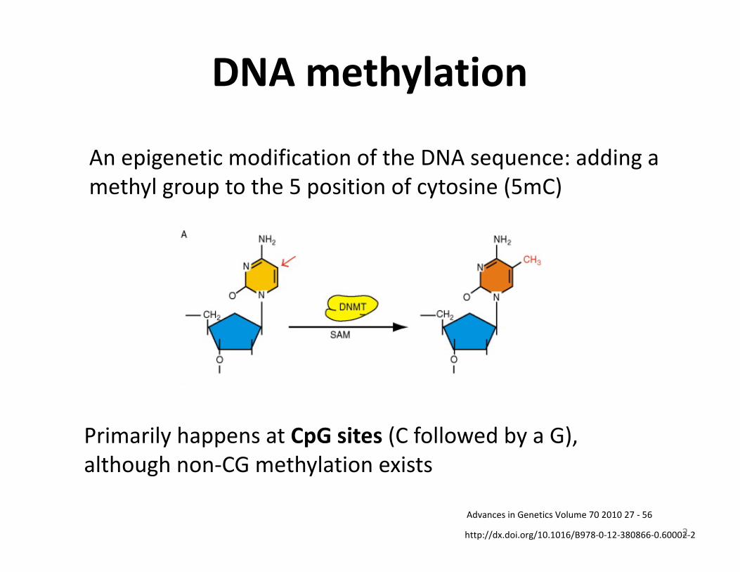
AnepigeneticmodificationoftheDNAsequence:addingamethylgrouptothe5positionofcytosine(5mC)

PrimarilyhappensatCpGsites(CfollowedbyaG),althoughnon-CGmethylationexists

DNAmethylation

2

Varley K E et al. Genome Res. 2013;23:555-567

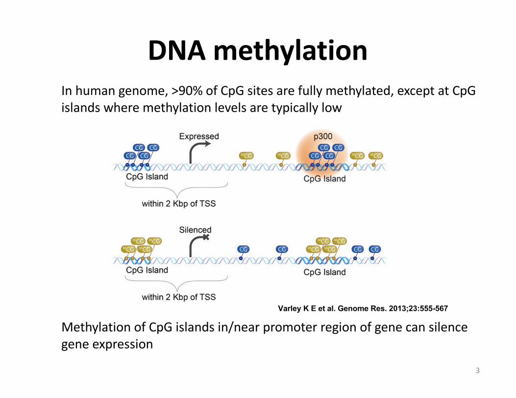
Inhumangenome,>90%ofCpGsitesarefullymethylated,exceptatCpGislandswheremethylationlevelsaretypicallylow

MethylationofCpGislandsin/nearpromoterregionofgenecansilencegeneexpression

DNAmethylation

3

• Importantingeneregulation– Methylationofpromoterregionscansuppressgeneexpression

• Playscrucialroleindevelopment– Heritableduringcelldivision

– Helpscellsestablishidentityduringcell/tissuedifferentiation

• Canbeinfluencedbyenvironment– GoodcandidatetomediateGxE interactions

FunctionofDNAmethylation

4

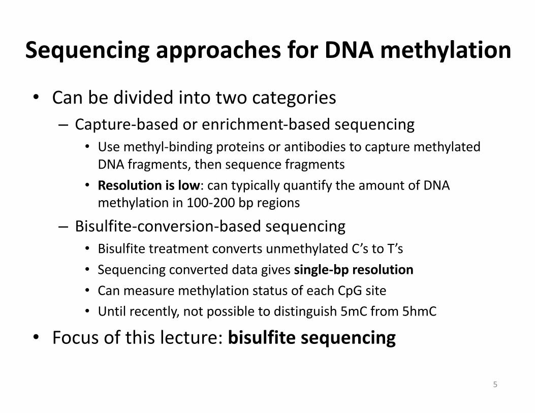
SequencingapproachesforDNAmethylation

• Canbedividedintotwocategories– Capture-basedorenrichment-basedsequencing

• Usemethyl-bindingproteinsorantibodiestocapturemethylatedDNAfragments,thensequencefragments

• Resolutionislow:cantypicallyquantifytheamountofDNAmethylationin100-200bp regions

– Bisulfite-conversion-basedsequencing• Bisulfitetreatmentconvertsunmethylated C’stoT’s• Sequencingconverteddatagivessingle-bp resolution• CanmeasuremethylationstatusofeachCpG site• Untilrecently,notpossibletodistinguish5mCfrom5hmC

• Focusofthislecture:bisulfitesequencing

5

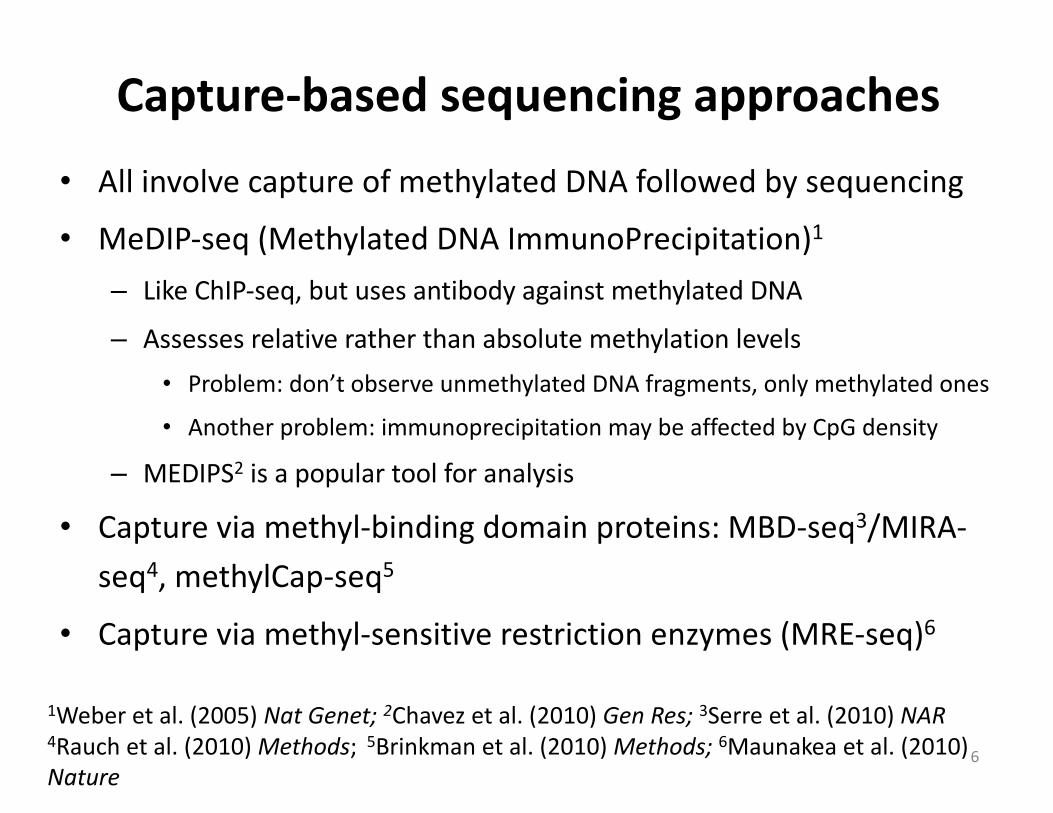
Capture-basedsequencingapproaches• AllinvolvecaptureofmethylatedDNAfollowedbysequencing

• MeDIP-seq (MethylatedDNAImmunoPrecipitation)1

– LikeChIP-seq,butusesantibodyagainstmethylatedDNA

– Assessesrelativeratherthanabsolutemethylationlevels• Problem:don’tobserveunmethylated DNAfragments,onlymethylatedones

• Anotherproblem:immunoprecipitation maybeaffectedbyCpG density

– MEDIPS2 isapopulartoolforanalysis

• Captureviamethyl-bindingdomainproteins:MBD-seq3/MIRA-seq4,methylCap-seq5

• Captureviamethyl-sensitiverestrictionenzymes(MRE-seq)6

6

1Weberetal.(2005)NatGenet;2Chavezetal.(2010)GenRes;3Serreetal.(2010)NAR4Rauchetal.(2010)Methods; 5Brinkmanetal.(2010)Methods; 6Maunakeaetal.(2010)Nature

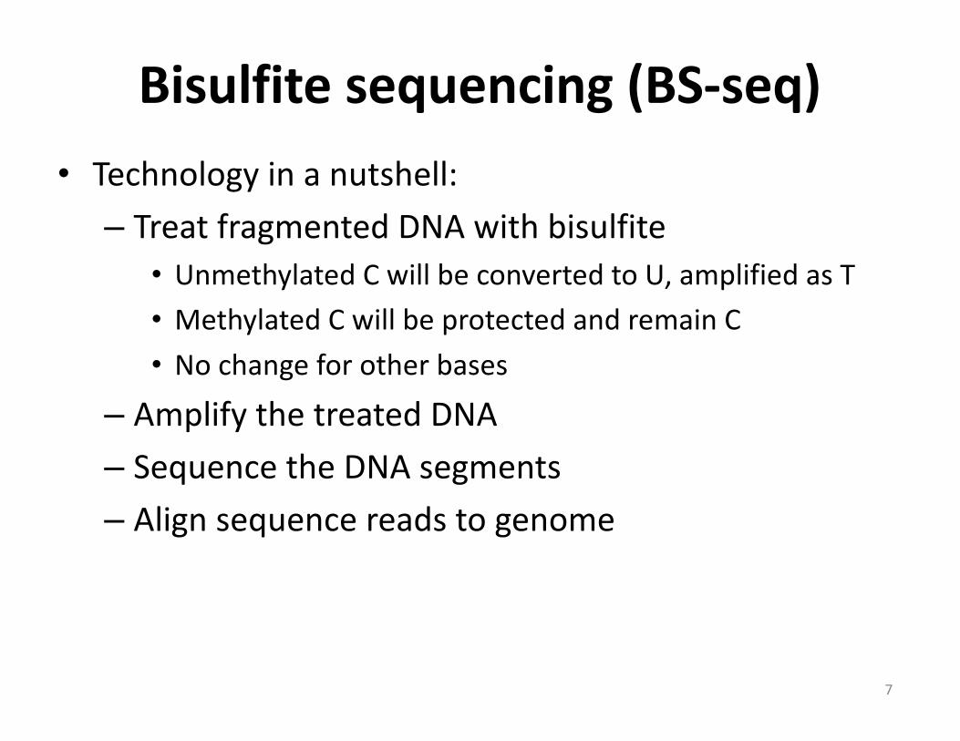
Bisulfitesequencing(BS-seq)• Technologyinanutshell:– TreatfragmentedDNAwithbisulfite

• Unmethylated CwillbeconvertedtoU,amplifiedasT• MethylatedCwillbeprotectedandremainC• Nochangeforotherbases

– AmplifythetreatedDNA– SequencetheDNAsegments– Alignsequencereadstogenome

7

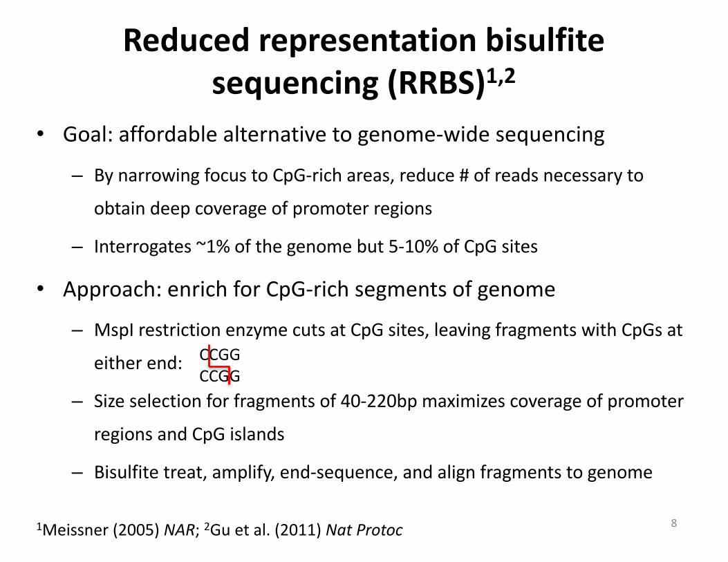
Reducedrepresentationbisulfitesequencing(RRBS)1,2

• Goal:affordablealternativetogenome-widesequencing

– BynarrowingfocustoCpG-richareas,reduce#ofreadsnecessaryto

obtaindeepcoverageofpromoterregions

– Interrogates~1%ofthegenomebut5-10%ofCpG sites

• Approach:enrichforCpG-richsegmentsofgenome

– MspI restrictionenzyme cutsatCpG sites,leavingfragmentswithCpGs at

eitherend:

– Sizeselectionforfragmentsof40-220bpmaximizescoverageofpromoter

regionsandCpG islands

– Bisulfitetreat,amplify,end-sequence,andalignfragmentstogenome

81Meissner(2005)NAR;2Guetal.(2011)NatProtoc

CCGGCCGG

IllustrationofbisulfiteconversionBMC Bioinformatics 2009, 10:232 http://www.biomedcentral.com/1471-2105/10/232

Page 2 of 9(page number not for citation purposes)

detect the methylation pattern of every C in the genome.Nevertheless, the mapping of millions of bisulfite reads tothe reference genome remains a computational challenge.

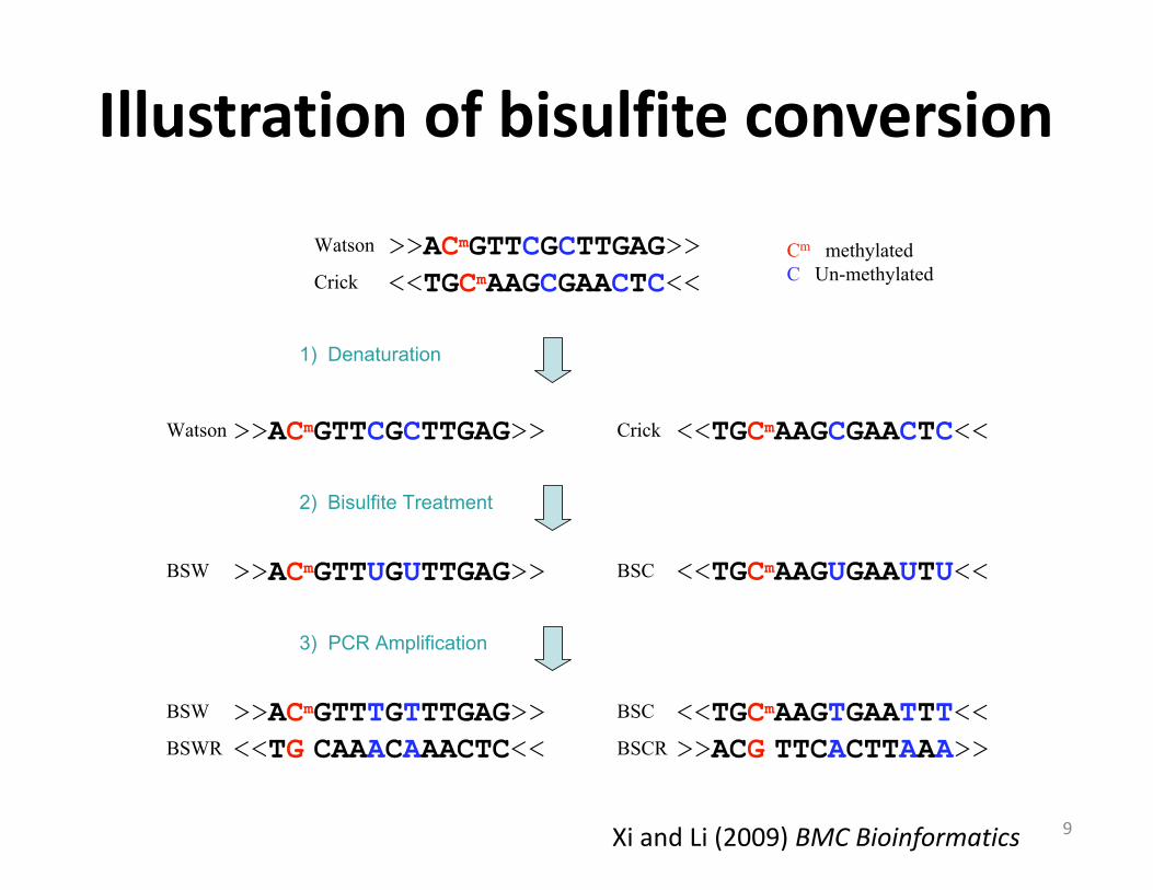
ProblemsFirst, the searching space is significantly increased relativeto the original reference sequence. Unlike normalsequencing, the Watson and Crick strands of bisulfite-treated sequences are not complementary to each otherbecause the bisulfite conversion only occurs on Cs. As aresult, there will be four distinct strands after PCR ampli-fication: BSW (bisulfite Watson), BSWR (reverse comple-ment of BSW), BSC (bisulfite Crick), and BSCR (reversecomplement of BSC) (Figure 1). During shotgun sequenc-ing, a bisulfite read is almost equally likely to be derivedfrom any of the four strands.

Second, sequence complexity is reduced. In the mamma-lian genome, although ~19% of the bases are Cs and

another 19% are Gs, only ~1.8% of dinucleotides are CpGdinucleotides. Because C methylation occurs almostexclusively at CpG dinucleotide, the vast majority of Cs inBSW and BSC strands will be converted to Ts. Therefore,most reads from the above two strands will be C-poor.However, PCR amplification will transcribe all Gs as Cs inBSWR and BSCR strands, so reads from those two strandsare typically G-poor and have a normal C content. As aresult, we expect the overall C content of bisulfite reads tobe reduced by ~50%.

Third, C to T mapping is asymmetric. The T in the bisulfitereads could be mapped to either C or T in the referencebut not vice versa. This phenomenon not only increasesthe search space for mapping but also complicates thematching process (Figure 2). Efficient implementation ofsuch asymmetric C/T matching is critical for mappinghigh-throughput bisulfite reads to the reference genome

Pipeline of bisulfite sequencingFigure 1Pipeline of bisulfite sequencing. 1) Denaturation: separating Watson and Crick strands; 2) Bisulfite treatment: converting un-methylated cytosines (blue) to uracils; methylated cytosines (red) remain unchanged; 3) PCR amplification of bisulfite-treated sequences resulting in four distinct strands: Bisulfite Watson (BSW), bisulfite Crick (BSC), reverse complement of BSW (BSWR), and reverse complement of BSC (BSCR).

>>ACmGTTCGCTTGAG>> <<TGCmAAGCGAACTC<<

Watson

Crick

Watson Crick

>>ACmGTTUGUTTGAG>> <<TGCmAAGUGAAUTU<<

<<TGCmAAGTGAATTT<<

>>ACG TTCACTTAAA>><<TG CAAACAAACTC<<

>>ACmGTTTGTTTGAG>>BSW

BSWR

BSW

BSC

BSCR

BSC

Cm methylatedC Un-methylated

1) Denaturation

2) Bisulfite Treatment

3) PCR Amplification

>>ACmGTTCGCTTGAG>>

<<TGCmAAGCGAACTC<<

XiandLi(2009)BMCBioinformatics 9

AlignmentofBS-seq• Problem:readscannotbedirectlyalignedtothereferencegenome.– FourdifferentstrandsafterbisulfitetreatmentandPCR– C-Tmismatcheswillmeanunmethylated readscan’tbealignedtothecorrectposition• Unmethylated CpGs willalignwithTpGs orlikelynotatall• Willleadtoastrongbiasinfavorofmethylatedreads

• Onepossiblesolutioninsilico bisulfiteconversion– SwitchallC’stoT’sinbothreadsandreferencesample– Usethisforalignment,thenchangebacktooriginal

10

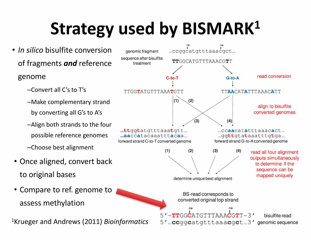
• Insilico bisulfiteconversionoffragmentsand referencegenome–ConvertallC’stoT’s

–MakecomplementarystrandbyconvertingallG’stoA’s

–Alignbothstrandstothefourpossiblereferencegenomes

–Choosebestalignment

• Oncealigned,convertbacktooriginalbases

• Comparetoref.genometoassessmethylation

StrategyusedbyBISMARK1

111KruegerandAndrews(2011)Bioinformatics

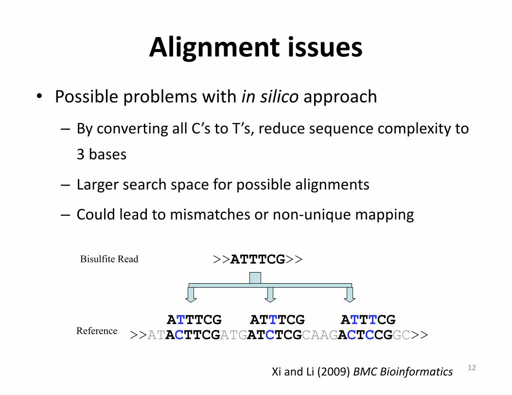
• Possibleproblemswithinsilico approach

– ByconvertingallC’stoT’s,reducesequencecomplexityto3bases

– Largersearchspaceforpossiblealignments

– Couldleadtomismatchesornon-uniquemapping

Alignmentissues

12

BMC Bioinformatics 2009, 10:232 http://www.biomedcentral.com/1471-2105/10/232

Page 3 of 9(page number not for citation purposes)

and is still lacking in current short read alignment soft-ware.

A common approach to overcome these issues is to con-vert all Cs to Ts and map the converted reads to the con-verted reference; then, the alignment results are post-processed to count false-positive bisulfite C/T alignmentsas mismatches, where a C in the BS-read is aligned to a Tin the reference [2]. Although this all-inclusive C/T con-version is effective for reads derived from the C-poorstrands, it is not appropriate for reads derived from the G-poor strands, where all the Cs are actually transcribedfrom Gs by PCR amplification and thus could not be con-verted to Ts during bisulfite treatment. During shotgunsequencing, however, a bisulfite read is almost equallylikely to be derived from either the C-poor or the G-poorstrands. There is no precise way to determine the original

strand a bisulfite read is derived from. Furthermore, byignoring the C/T mapping asymmetry, this strategy gener-ates a large number of false-positive bisulfite mappingsand greatly increases the computational load in a quad-ratic manner with an increase in the size of the referencesequence. In order to accurately extract the true bisulfitemappings in the post-processing stage, all mapping loca-tions have to be recorded, even the non-unique map-pings. Therefore, this approach is only practical for smallreference sequences, where only the C-poor strands aresequenced. For example, Meissner et al. used this map-ping strategy for reduced representation bisulfite sequenc-ing (RRBS) [2], where the genomic DNA was digested bythe Mspl restriction enzyme and 40–220 bp segmentswere selected for sequencing. The reference sequence (~27M nt) is only about 1% of the whole mouse genome, cov-ering 4.8% of the total CpG dinucleotides.

Mapping of bisulfite readsFigure 2Mapping of bisulfite reads. 1) Increased search space due to the cytosine-thymine conversion in the bisulfite treatment. 2) Mapping asymmetry: thymines in bisulfite reads can be aligned with cytosines in the reference (illustrated in blue) but not the reverse.

>>ATTTCG>>

>>ATACTTCGATGATCTCGCAAGACTCCGGC>>

ATTTCG ATTTCGATTTCG

Bisulfite Read

Reference

Bisulfite Read Reference

C

T

C

T

1) Multiple Mapping

2) Mapping AsymmetryXiandLi(2009)BMCBioinformatics

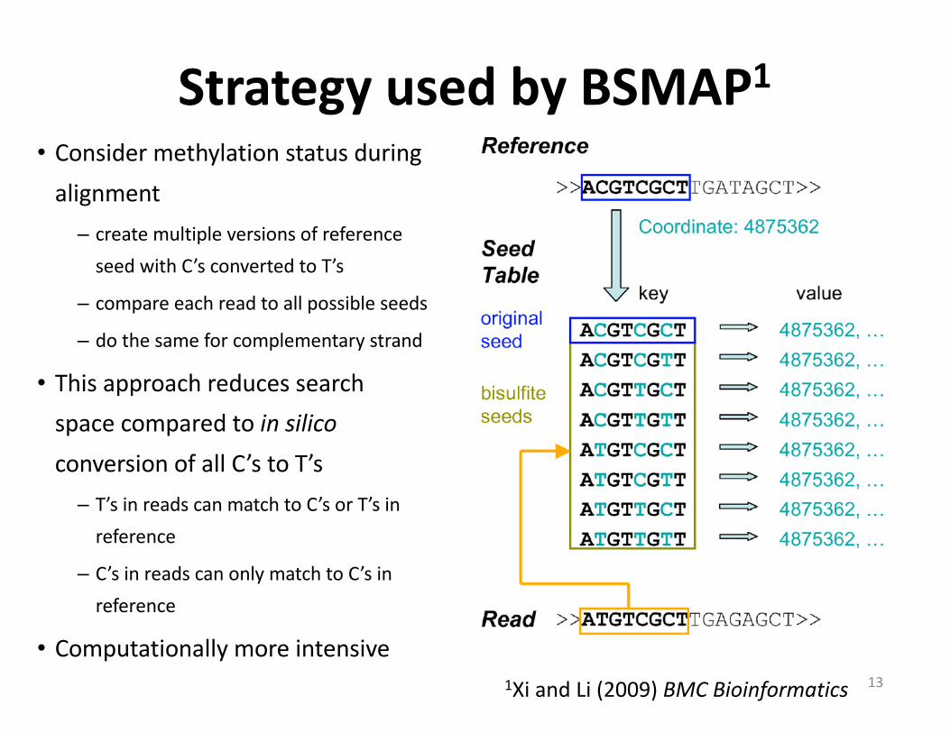
• Considermethylationstatusduringalignment– createmultipleversionsofreferenceseedwithC’sconvertedtoT’s

– compareeachreadtoallpossibleseeds

– dothesameforcomplementarystrand

• ThisapproachreducessearchspacecomparedtoinsilicoconversionofallC’stoT’s– T’sinreadscanmatchtoC’sorT’sinreference

– C’sinreadscanonlymatchtoC’sinreference

• Computationallymoreintensive

StrategyusedbyBSMAP1

131XiandLi(2009)BMCBioinformatics

Whichalignmentsoftwareisbest?

14

• AdvantagesofBSMAP:– reducessearchspacebyeliminatingmappingofC’stoT’s

– greaterproportionofuniquelymappingreads1

• AdvantagesofBISMARK:– muchfasterthanBSMAPandotherprograms1

– uniquenessofmappingindependentofmethylationstatus1

– moreuser-friendlyintermsofextractingdata,interfacingwithothersoftware1

• Ingeneral,BISMARKseemstobethepopularchoice

1Chatterjeeetal.(2012)NAR

Otheraligners

15

• AlignmentofRRBSdata

– Chatterjee etal.notesitismuchfasterifweuseinformationonMspI cutpoints to“reduce”referencegenomeinsilico1

– RRBSMAP:aversionofBSMAPthatdoesexactlythat2

– Hasoptiontoworkwithdifferentrestrictionenzymes

• Manyotheralignersforbisulfitesequencingdata

– OneusefulreviewoftheseisHackenberg etal.3

1Chatterjeeetal.(2012)NAR;2Xietal.(2012)Bioinformatics;3Hackenbergetal.(2012):Chapter2in“DNAMethylation– FromGenomicstoTechnology”Tatarinova (Ed.)http://www.intechopen.com/books

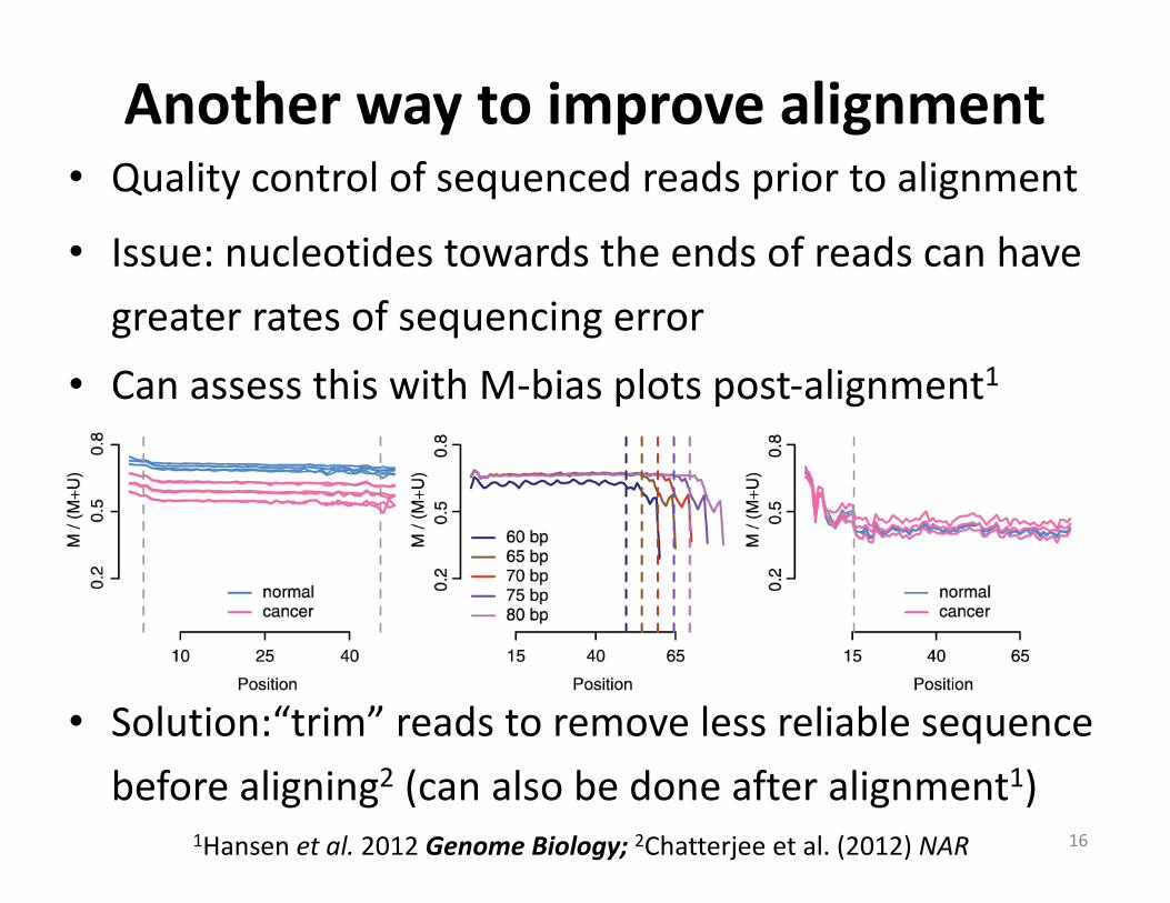
Anotherwaytoimprovealignment

16

• Qualitycontrolofsequencedreadspriortoalignment

• Issue:nucleotidestowardstheendsofreadscanhavegreaterratesofsequencingerror

• CanassessthiswithM-biasplotspost-alignment1

• Solution:“trim”readstoremovelessreliablesequencebeforealigning2 (canalsobedoneafteralignment1)

1Hansenetal.2012GenomeBiology;2Chatterjeeetal.(2012)NAR

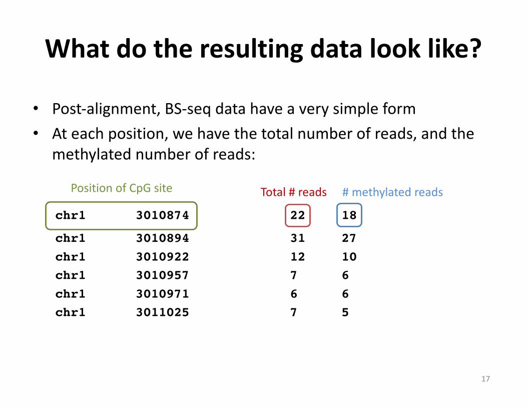
• Post-alignment,BS-seq datahaveaverysimpleform• Ateachposition,wehavethetotalnumberofreads,andthe

methylatednumberofreads:

chr1 3010874 22 18

chr1 3010894 31 27chr1 3010922 12 10chr1 3010957 7 6chr1 3010971 6 6chr1 3011025 7 5

Total#reads #methylatedreadsPositionofCpG site

Whatdotheresultingdatalooklike?

17

StudydesignforBS-seq studies• Highcostsà fewsamplestypicallyanalyzed• Twocommonstudydesigns– Analysisofasinglesample:

• Goal:observemethylationpatternsacrossgenome• Commonlydonetocharacterizemethylome foraparticularcelltypeorspecies

– Comparisonofseveralsamples:• Typicalgoal:comparemethylationlevelsbetweengroups• Differentialmethylationanalysis• ComparedwithChIP-seq andRNA-seq,methodsarestillinearlystage,andareoftenadhoc

18

StudydesignforBS-seq studies• Becausesofewsamplesareinvolvedinmoststudies,itiscrucialtoavoidallformsofheterogeneity– Inlargestudieswecanadjustfordifferencesviacovariates– WithsmallNmodelsoftencannotaccommodatecovariates

• Heterogeneity=differencesbetweensamplesotherthanvariableofinterest– Inadvertentdifferencesintissuesampled– Differencesincelltypemixingproportions– Geneticdifferencesbetweenindividuals– Agedifferencesbetweensamples– Different#ofpassagesforcelllines

19

Avoidingheterogeneity• Canavoidheterogeneitywithcarefulstudydesign

– Stringentcontroloftissuedissectionfortissuesampling

– Analysisofhomogeneouscelltypeswheneverpossible

– Useofwithin-individualcomparisonstoavoidgeneticand

demographicdifferences

• Example:pairedtumorandnormalsamplesfromsamepatients

• Ifnotpossible,matchcarefullyforethnicity,age,gender

– Carefulcontrolofcelllineexperiments

20

QualitycontrolofalignedBS-seq data

21

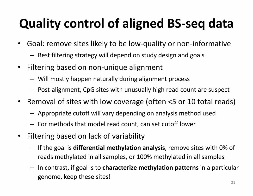
• Goal:removesiteslikelytobelow-qualityornon-informative– Bestfilteringstrategywilldependonstudydesignandgoals

• Filteringbasedonnon-uniquealignment– Willmostlyhappennaturallyduringalignmentprocess– Post-alignment,CpG siteswithunusuallyhighreadcountaresuspect

• Removalofsiteswithlowcoverage(often<5or10totalreads)– Appropriatecutoffwillvarydependingonanalysismethodused– Formethodsthatmodelreadcount,cansetcutofflower

• Filteringbasedonlackofvariability– Ifthegoalisdifferentialmethylationanalysis,removesiteswith0%of

readsmethylatedinallsamples,or100%methylatedinallsamples– Incontrast,ifgoalistocharacterizemethylationpatternsinaparticular

genome,keepthesesites!

Differentialmethylationanalysis• Typicalgoal:comparemethylationlevelsbetweentwogroups– Example:tumorvs.normaltissuesamples

– Important:dogroupscontainbiologicalreplicates?

– Somestudiesmaycompare1tumorto1normalsample

– Otherstudieswillinclude2ormorereplicatesofeach

• PopularadhocapproachesforthiscomparisonareFisher’sexacttestandtwo-groupt-test

• Wewillshowwhythesecanbeproblematic

22

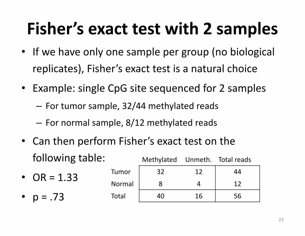
Fisher’sexacttestwith2samples• Ifwehaveonlyonesamplepergroup(nobiologicalreplicates),Fisher’sexacttestisanaturalchoice

• Example:singleCpG sitesequencedfor2samples– Fortumorsample,32/44methylatedreads

– Fornormalsample,8/12methylatedreads

• CanthenperformFisher’sexacttestonthefollowingtable:

• OR=1.33

• p=.73

Methylated Unmeth. Totalreads

Tumor 32 12 44

Normal 8 4 12

Total 40 16 56

23

Fisher’sexacttestinmethylKit• Forcomparisonsbetweentwosamples,Fisher’sexacttestisareasonablechoice– EasytocarryoutinRusingfisher.test()function

– Alternatively,methylKit1 isasuiteofRfunctionsthatfacilitatesanalysisofgenome-widemethylationdata

– Differentialmethylationanalysisviaeither• Fisher’sexacttest(forcomparisonsbetweentwosamples)

• Logisticregressionbasedonmethylationproportions– Analogoustotwo-groupt-test,butwithcovariates

• Canperformanalysisinuser-definedtilingwindows– However,basedonsimplecollapsingofinformationacrosssitesratherthan

smoothing241Akalinetal.2012GenomeBiology

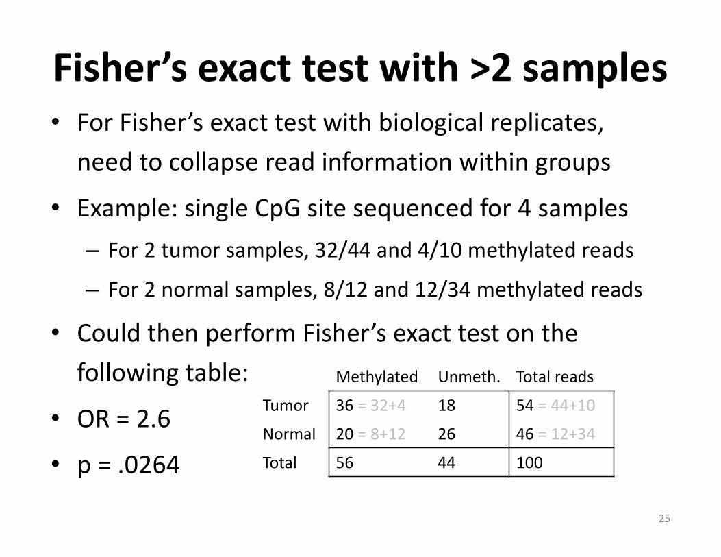
Fisher’sexacttestwith>2samples• ForFisher’sexacttestwithbiologicalreplicates,needtocollapsereadinformationwithingroups

• Example:singleCpG sitesequencedfor4samples– For2tumorsamples,32/44and4/10methylatedreads

– For2normalsamples,8/12and12/34methylatedreads

• CouldthenperformFisher’sexacttestonthefollowingtable:

• OR=2.6

• p=.0264

Methylated Unmeth. Totalreads

Tumor 36=32+4 18 54 =44+10

Normal 20= 8+12 26 46 =12+34

Total 56 44 100

25

ProblemwithFisher’sexacttest• ToperformFisher’sexacttestfor>2samples,wehaveto

collapsereadinformationacrosssampleswithineachgroup

• Bydoingthis,weareignoringinformationonbiologicalvariationbetweensamples– Biologicalvariation:naturalvariationinunderlyingfractionofDNA

methylatedbetweensamplesinthesamecondition

– Technicalvariation:variationinestimationofmethylationlevelsduetorandomsamplingofDNAduringsequencing1

• Bycollapsing,weareassumingthat:– sampleswithinagroupinherentlyhavethesameunderlying

fractionofDNAmethylated

– anyvariationbetweensamplesisduetotechnicalvariation

261Hansenetal.2012GenomeBiology

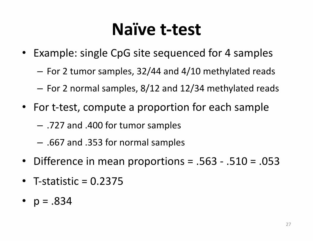
Naïvet-test• Example:singleCpGsitesequencedfor4samples

– For2tumorsamples,32/44and4/10methylatedreads

– For2normalsamples,8/12and12/34methylatedreads

• Fort-test,computeaproportionforeachsample– .727and.400fortumorsamples

– .667and.353fornormalsamples

• Differenceinmeanproportions=.563- .510=.053

• T-statistic=0.2375

• p=.834

27

Problemwitht-test• Toperformt-test,computedaproportionforeachsample

– Testinherentlygivesequalweighttoeachsample

– Doesnotaccountfortechnicalvariationinproportionestimates

– Recall:Technicalvariation=variationinestimationofmethylationlevelsduetorandomsamplingofDNA

– Canexpectthisvariationtobelowerforsampleswithmorereads

• Onepossiblesolutionwouldbetoincorporateweightsbasedonreadcount

• However,anotherissuewiththisapproachisthesmallnumberofsamples– WithN=4,thet-testhasverylittlepowerduetolowdf

28

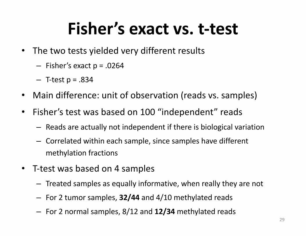
Fisher’sexactvs.t-test• Thetwotestsyieldedverydifferentresults

– Fisher’sexactp=.0264

– T-testp=.834

• Maindifference:unitofobservation(readsvs.samples)

• Fisher’stestwasbasedon100“independent”reads– Readsareactuallynotindependentifthereisbiologicalvariation

– Correlatedwithineachsample,sincesampleshavedifferentmethylationfractions

• T-testwasbasedon4samples– Treatedsamplesasequallyinformative,whenreallytheyarenot

– For2tumorsamples,32/44and4/10methylatedreads

– For2normalsamples,8/12and12/34methylatedreads29

Needbetterapproaches• Problem:wanttotestmanysiteswithfewsamples

– Limitedinformationavailableateachsiteduetolow#ofsamples

• Solution:approachesthatborrowinformationacrosssites

– Smoothingapproachesthatshareinformationacrossnearbysites

• Usefulinsinglesampleanalysesthataimtocharacterizethegenome

• Usefulfordetectingdifferentialmethylatedregions(DMRs)ofthegenome

– Bayesianhierarchicalmodelthatborrowsinformationacrossthe

genome

• Usefulfordetectingdifferentiallymethylatedloci(DMLs)

30

Smoothingapproaches

• Firstconsideranalysisofasinglesample

• Goalhereistoidentifymethylatedregionsorloci:– CanestimateproportionofreadsthataremethylatedateachCposition,but:

• Variabilityinestimationneedstobeconsidered

• SpatialcorrelationamongnearbyCpG sitescanbeutilizedtoimproveestimation

– Methylatedregions(orstates)canbedeterminedbysmoothingbasedmethodsusingtheestimatedmethylationproportionasinput

31

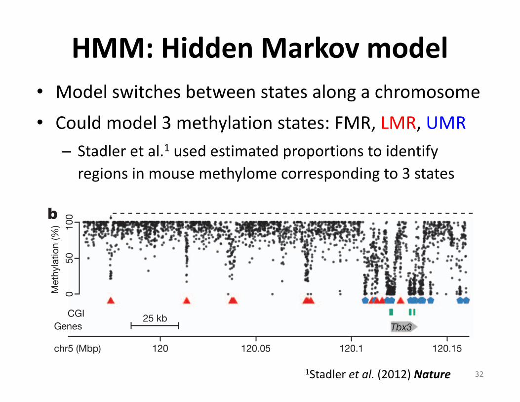
HMM:HiddenMarkovmodel• Modelswitchesbetweenstatesalongachromosome• Couldmodel3methylationstates:FMR,LMR,UMR

– Stadleretal.1 usedestimatedproportionstoidentifyregionsinmousemethylomecorrespondingto3states

DNase-I-hypersensitive sites (DHS), a unique chromatin state thatdepends on DNA-binding factors10–12. In fact, at least 80% of LMRsand 90% of UMRs overlap with DHS (Fig. 2 and SupplementaryFig. 2). LMRs are unlikely novel promoters as we find only weak signalfor RNA polymerase II (Fig. 2 and Supplementary Fig. 3) and no RNAsignal abovewhat we observe atmethylated regions evenwhen using astrand-specific protocol that does not require polyadenylation (Sup-plementary Fig. 3). Next, we explored if LMRs could represent distalregulatory regions, such as enhancers. Indeed, LMRs are stronglyenriched for chromatin features such as highH3K4monomethylation(H3K4me1) signal relative to H3K4 trimethylation (H3K4me3) andthe presence of p300 histone acetyltransferase, which are predictivefeatures of enhancers13 (Fig. 2). This indicates that a subset of LMRsare enhancers that, in light of the absence of H3K27me3 and thepresence of H3K27ac, are presumably active14 (Fig. 2b). Transgenicassays further show that individual LMRs increase the activity of alinked promoter and experimentally function as enhancers (Sup-plementary Fig. 4). We thus conclude that many LMRs, identifiedsolely by their DNA methylation pattern, represent active regulatoryregions.To investigate LMR features further, we combined newly generated

and published data sets for several DNA-binding factors and addi-tional histone modifications (Supplementary Table 1, Fig. 2b andSupplementary Figs 5 and 6). LMRs and UMRs are depleted for theheterochromatic histone modification H3K9me2 in agreement withthe absence of this mark at active chromatin6. Most DNA-bindingfactors show enrichment not only at UMRs, which are mostly pro-moters, but also at LMRs. Factors enriched at LMRs in stem cellsinclude pluripotency transcription factors such as Nanog, Oct4 andKlf4, but also structural DNA-binding factors such as the insulator

protein CTCF15 and members of the cohesin complex (Fig. 2b andSupplementary Fig. 5), both of which bind promoters and distalregulatory regions16. Notably, not all factors occupy distal andproximal regulatory regions with equal preferences. Smad1 binds toneither LMRs nor UMRs, whereas some bind primarily at UMRs, suchas KDM2A and Zfx, and others such as Nanog and Esrrb show higherenrichment at LMRs (Fig. 2b and Supplementary Fig. 5). In summary,several lines of evidence including genomic position, conservation,chromatin state, regulatory activity and transcription factor occupancysupport the hypothesis that LMRs are indeed active distal regulatoryregions.InterestinglyLMRsshowastrongpresenceof5-hydroxymethylcytosine

(5hmC), consistent with recent reports of 5hmC presence at enhancerregions17–19. One candidate protein responsible for catalysing 5hmC,Tet1 (refs 20, 21), is enriched at both UMRs and LMRs (Fig. 2b).To ask if LMRs are also present in other mammals we performed

HMM segmentation of a human stem cell methylome3, which alsoidentifies LMRswith similar features, indicating that these are a generalcharacteristic of mammalian methylomes (Supplementary Fig. 7).

Transcription factor binding creates LMRsTodetermine howLMRs are formed,we investigated theDNA-bindingprotein CTCF, which binds to regulatory regions including promoters,enhancers and insulators22,23.Wedetermined the genome-wide bindingof CTCF by chromatin immunoprecipitation followed by sequencing(ChIP-seq) (Supplementary Fig. 8), revealing high occupancy at bothUMRs and LMRs (Fig. 2b and Supplementary Fig. 5). A composite viewof DNA methylation shows an average methylation of 20% at CTCFbinding sites with increasing methylation adjacent to it (Supplemen-tary Fig. 9), in line with a previous report in primates24. If reducedmethylation is a general feature of CTCF-occupied sites, inclusion ofDNA methylation data should improve prediction of CTCF binding.

020

4060

8010

0M

ethy

latio

n (%

)

01

23

Enric

hmen

t

FMR UMR LMR

Tet15hmC.GLIB5hmC.CMSSmad1STAT3n-MycZfxKDM2AE2f1EsrrbKlf4NanogOct4Smc3Smc1NipblCTCFH3K27acH3K27me3H3K9me2p300Pol IIH3K4me3H3K4me2H3K4me1DNase IMethylation

a

b

UMRLMR

FMR

Mea

n co

nser

vatio

n Conservation

0 3–3 3–3 3–3

3–3 3–3 3–3

0.1

0.2

0.3

Enric

hmen

t (lo

g 2)

0

DNase I

0.0

0.5

1.0

1.5

Position around segment middle (kb)

Enric

hmen

t (lo

g 2)

00

00

H3K4me3 Pol II

H3K4me1 p300

0.0

0.5

1.0

0.0

1.0

2.0 1.

50.

00.

51.

01.

5

0.0

0.3

0.6

0.9

Figure 2 | General features of LMRs. Composite profiles 3 kb aroundsegment midpoints. a, Evolutionary conservation based on multi-speciesalignments (upper left). Enrichment of DNase I tags (lower left). Chromatinfeatures that predict enhancer function are enriched at LMRs (middle andright). b, Heat map of methylation levels, histone modifications and proteinbinding (H3K4me1 signal rescaled for visibility).

a c d

e f

b

025

5075

100

Met

hyla

tion

(%)

FMRLMRUMR

−3 0 3

Position around middle (kb)

0 5 10 15 20

0.00

0.10

Distance to TSS (log2 nt)

Den

sity

FMRLMRUMR

12

22

44

32

FMR(2,485.0 Mbp)

57

3

13 7

20

UMR(27.9 Mbp)

34

25

34

33

LMR(12.0 Mbp)

Promoter Exon Intron Repeat Intergenic

89 (1)

2 (1)9 (98)

CpG islands

FMR UMR LMR

(n = 15,974)

Methylation (%)

Frac

tion

of C

pGs

0.0

0.25

0.5

0−10

10−2

0

20−3

0

30−4

0

40−5

0

50−6

0

60−7

0

70−8

0

80−9

0

90−1

00

6.5% 4.1% 89.4%0

5010

0M

ethy

latio

n (%

)

CGITbx3

120 120.05 120.1 120.15chr5 (Mbp)

Genes

LMR

25 kb

Figure 1 | Features of the mouse ES cell methylome. a, Distribution of CpGmethylation frequency for all CpGs with at least tenfold coverage. Of allcytosines, 4.1% show intermediate methylation levels. b, Representativegenomic region. Computational segmentation identifies UMRs (bluepentagons), LMRs (red triangles) and FMRs (unmarked). Each dot representsone CpG (CpG islandsmarked in green). Included is an independently verifiedLMR upstream of Tbx3. Mbp, million base pairs. c, Composite profile of CpGmethylation for all three groups. kb, kilobases. d, Distances to TSS.e, f, Distribution of all three classes among genome features. e, A smallpercentage of LMRs overlap with CpG islands. Numbers indicate observedpercentage of overlaps per group (expected percentage in parentheses).f, Distribution of the regions throughout the genome.

ARTICLE RESEARCH

2 2 / 2 9 D E C E M B E R 2 0 1 1 | V O L 4 8 0 | N A T U R E | 4 9 1

Macmillan Publishers Limited. All rights reserved©2012

321Stadleretal.(2012)Nature

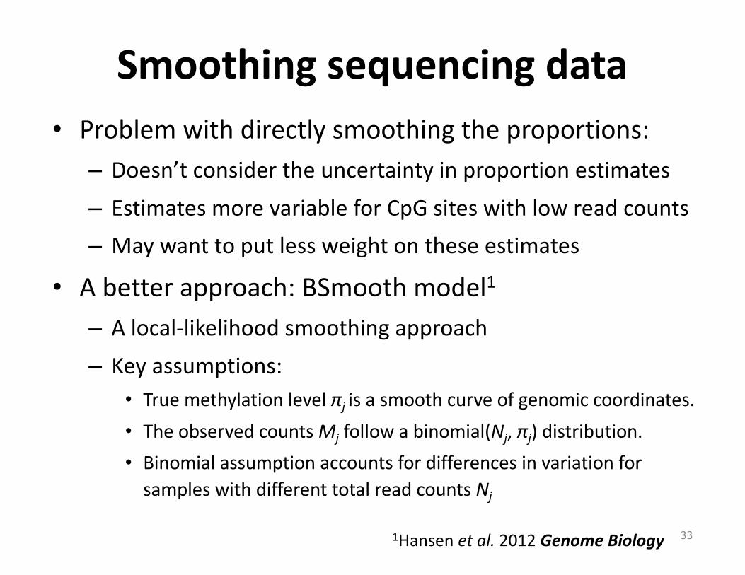
Smoothingsequencingdata• Problemwithdirectlysmoothingtheproportions:

– Doesn’tconsidertheuncertaintyinproportionestimates– EstimatesmorevariableforCpG siteswithlowreadcounts– Maywanttoputlessweightontheseestimates

• Abetterapproach:BSmooth model1

– Alocal-likelihoodsmoothingapproach– Keyassumptions:

• Truemethylationlevelπjisasmoothcurveofgenomiccoordinates.• TheobservedcountsMj followabinomial(Nj,πj)distribution.• BinomialassumptionaccountsfordifferencesinvariationforsampleswithdifferenttotalreadcountsNj


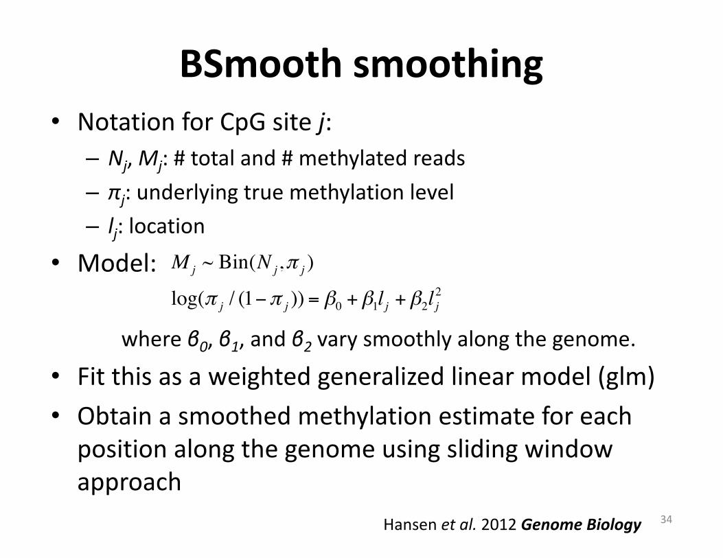
BSmoothsmoothing• NotationforCpG sitej:

– Nj,Mj:#totaland#methylatedreads– πj:underlyingtruemethylationlevel– lj:location

• Model:

whereβ0,β1,andβ2 varysmoothlyalongthegenome.

• Fitthisasaweightedgeneralizedlinearmodel(glm)• Obtainasmoothedmethylationestimateforeachpositionalongthegenomeusingslidingwindowapproach

M j ~ Bin(N j,π j )

log(π j / (1−π j )) = β0 +β1l j +β2l j2


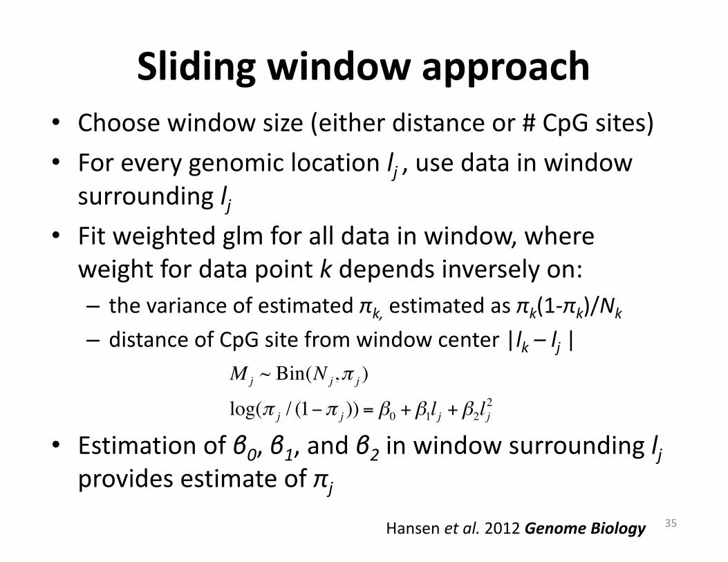
Slidingwindowapproach• Choosewindowsize(eitherdistanceor#CpGsites)• Foreverygenomiclocationlj,usedatainwindowsurroundinglj

• Fitweightedglmforalldatainwindow,whereweightfordatapointk dependsinverselyon:– thevarianceofestimatedπk, estimatedasπk(1-πk)/Nk

– distanceofCpGsitefromwindowcenter|lk – lj |

• Estimationofβ0,β1,andβ2 inwindowsurroundingljprovidesestimateofπj

M j ~ Bin(N j,π j )

log(π j / (1−π j )) = β0 +β1l j +β2l j2


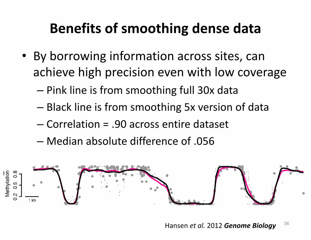
Benefitsofsmoothingdensedata

• Byborrowinginformationacrosssites,canachievehighprecisionevenwithlowcoverage– Pinklineisfromsmoothingfull30xdata– Blacklineisfromsmoothing5xversionofdata– Correlation=.90acrossentiredataset–Medianabsolutedifferenceof.056


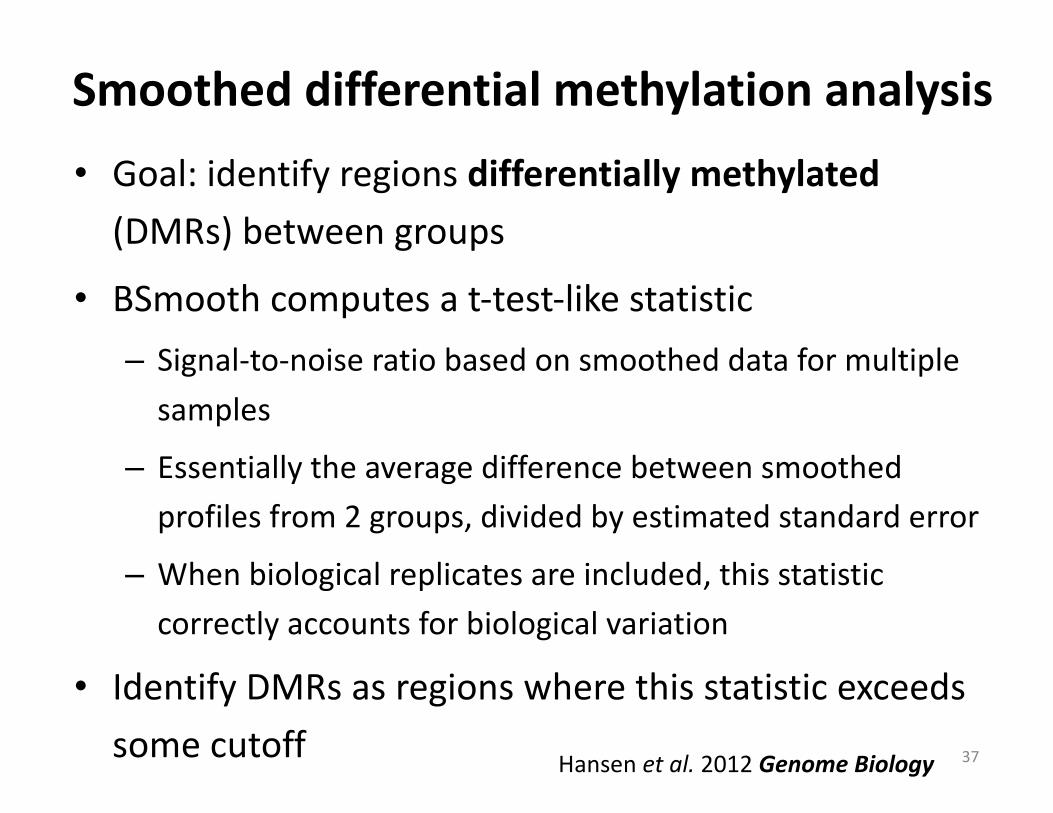
Smootheddifferentialmethylationanalysis• Goal:identifyregionsdifferentiallymethylated(DMRs)betweengroups

• BSmooth computesat-test-likestatistic– Signal-to-noiseratiobasedonsmootheddataformultiplesamples

– Essentiallytheaveragedifferencebetweensmoothedprofilesfrom2groups,dividedbyestimatedstandarderror

– Whenbiologicalreplicatesareincluded,thisstatisticcorrectlyaccountsforbiologicalvariation

• IdentifyDMRsasregionswherethisstatisticexceedssomecutoff 37Hansenetal.2012GenomeBiology

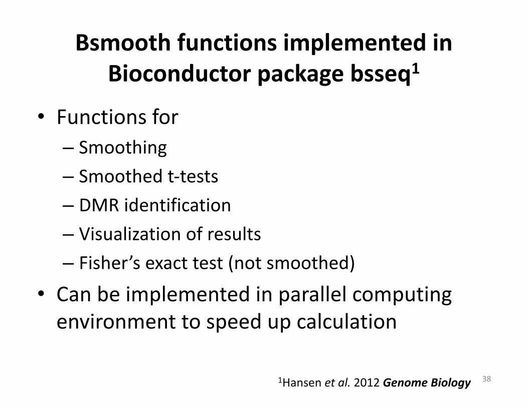
BsmoothfunctionsimplementedinBioconductorpackagebsseq1

• Functionsfor– Smoothing– Smoothedt-tests– DMRidentification– Visualizationofresults– Fisher’sexacttest(notsmoothed)

• Canbeimplementedinparallelcomputingenvironmenttospeedupcalculation


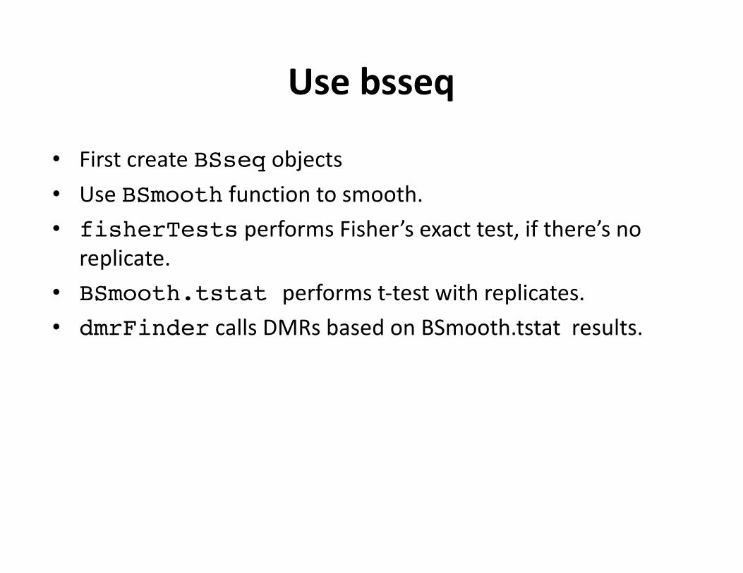
Usebsseq

• FirstcreateBSseq objects• UseBSmooth functiontosmooth.• fisherTests performsFisher’sexacttest,ifthere’sno

replicate.• BSmooth.tstat performst-testwithreplicates.• dmrFinder callsDMRsbasedonBSmooth.tstat results.

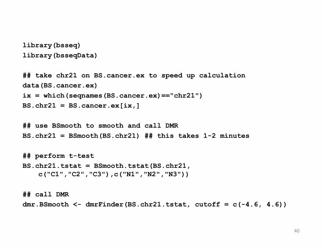
library(bsseq)library(bsseqData)

## take chr21 on BS.cancer.ex to speed up calculationdata(BS.cancer.ex)ix = which(seqnames(BS.cancer.ex)=="chr21")BS.chr21 = BS.cancer.ex[ix,]

## use BSmooth to smooth and call DMRBS.chr21 = BSmooth(BS.chr21) ## this takes 1-2 minutes

## perform t-testBS.chr21.tstat = BSmooth.tstat(BS.chr21,

c("C1","C2","C3"),c("N1","N2","N3"))

## call DMRdmr.BSmooth <- dmrFinder(BS.chr21.tstat, cutoff = c(-4.6, 4.6))

40

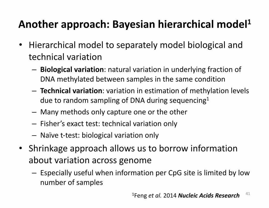
Anotherapproach:Bayesianhierarchicalmodel1

• Hierarchicalmodeltoseparatelymodelbiologicalandtechnicalvariation– Biologicalvariation:naturalvariationinunderlyingfractionof

DNAmethylatedbetweensamplesinthesamecondition– Technicalvariation:variationinestimationofmethylationlevels

duetorandomsamplingofDNAduringsequencing1

– Manymethodsonlycaptureoneortheother– Fisher’sexacttest:technicalvariationonly– Naïvet-test:biologicalvariationonly

• Shrinkageapproachallowsustoborrowinformationaboutvariationacrossgenome– EspeciallyusefulwheninformationperCpG siteislimitedbylow

numberofsamples411Fengetal.2014NucleicAcidsResearch

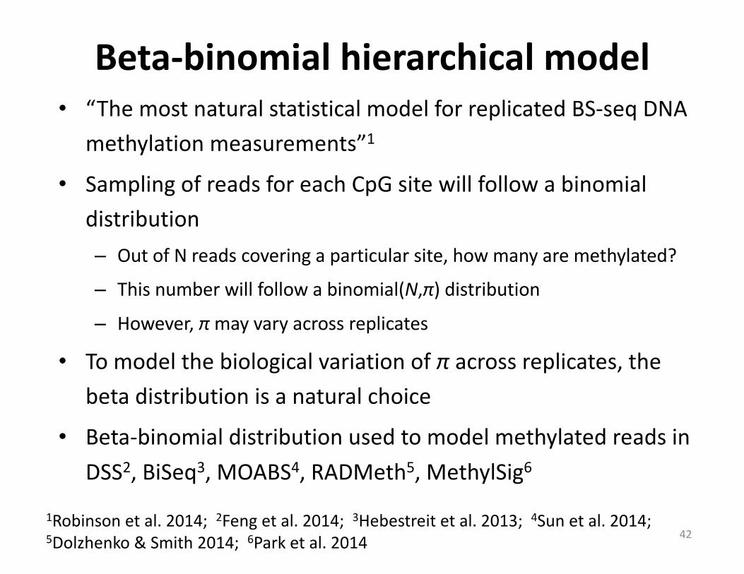
Beta-binomialhierarchicalmodel• “ThemostnaturalstatisticalmodelforreplicatedBS-seq DNA

methylationmeasurements”1

• SamplingofreadsforeachCpG sitewillfollowabinomialdistribution– OutofNreadscoveringaparticularsite,howmanyaremethylated?

– Thisnumberwillfollowabinomial(N,π)distribution

– However,πmayvaryacrossreplicates

• Tomodelthebiologicalvariationofπacrossreplicates,thebetadistributionisanaturalchoice

• Beta-binomialdistributionusedtomodelmethylatedreadsinDSS2,BiSeq3,MOABS4,RADMeth5,MethylSig6

421Robinsonetal.2014;2Fengetal.2014;3Hebestreitetal.2013;4Sunetal.2014;5Dolzhenko&Smith2014;6Parketal.2014

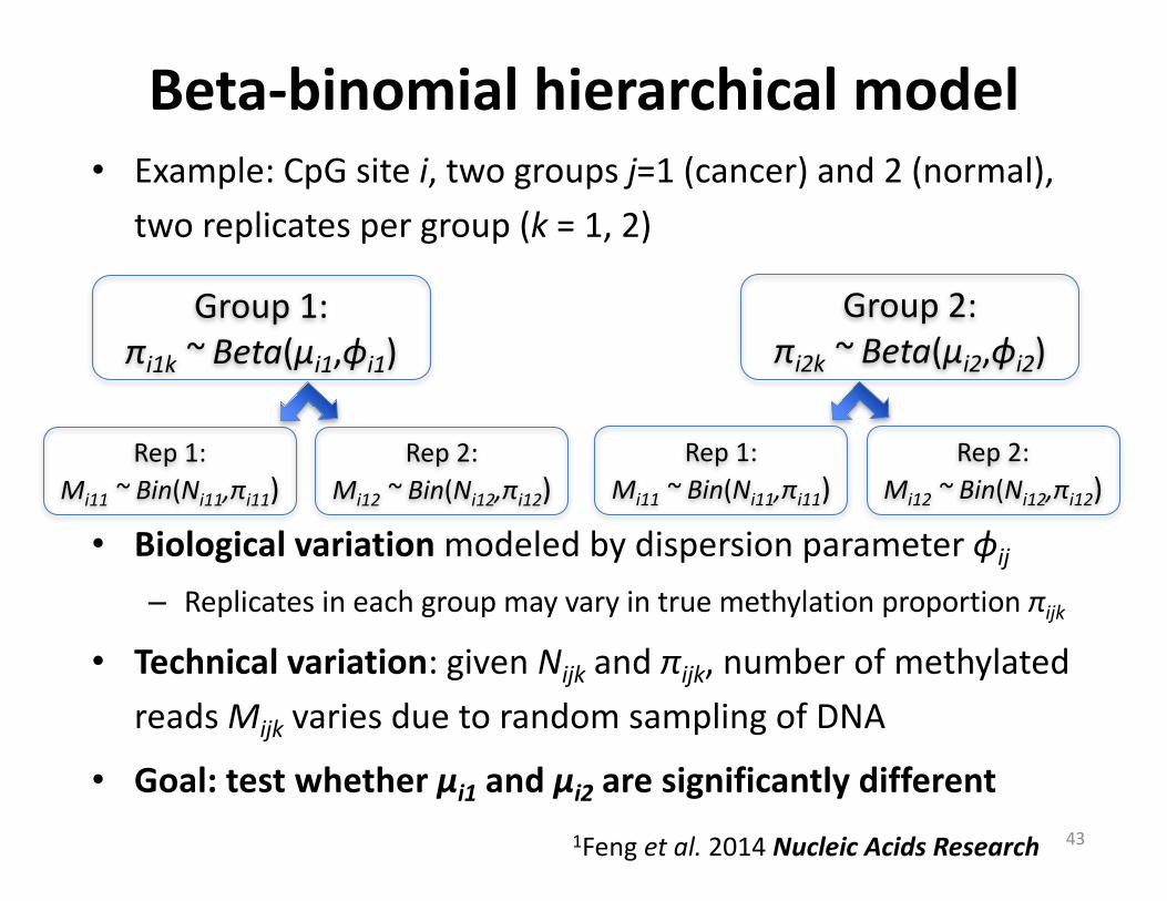
Beta-binomialhierarchicalmodel• Example:CpG sitei,twogroupsj=1(cancer)and2(normal),

tworeplicatespergroup(k =1,2)

• Biologicalvariationmodeledbydispersionparameterϕij

– Replicatesineachgroupmayvaryintruemethylationproportionπijk

• Technicalvariation:givenNijk andπijk,numberofmethylatedreadsMijk variesduetorandomsamplingofDNA

• Goal:testwhetherμi1 andμi2 aresignificantlydifferent43

Group1:πi1k ~Beta(μi1,ϕi1)

Group2:πi2k ~Beta(μi2,ϕi2)

Rep1:Mi11 ~Bin(Ni11,πi11)




1Fengetal.2014NucleicAcidsResearch

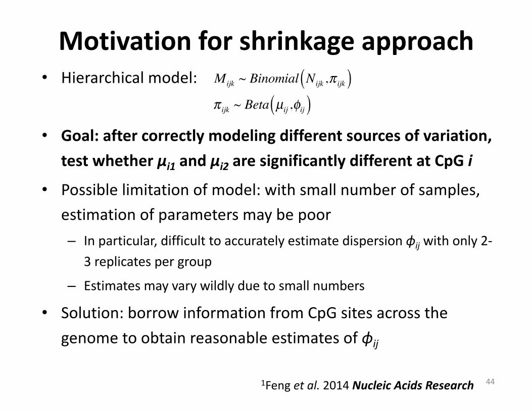
Motivationforshrinkageapproach• Hierarchicalmodel:

• Goal:aftercorrectlymodelingdifferentsourcesofvariation,testwhetherμi1 andμi2 aresignificantlydifferentatCpG i

• Possiblelimitationofmodel:withsmallnumberofsamples,estimationofparametersmaybepoor– Inparticular,difficulttoaccuratelyestimatedispersionϕij withonly2-

3replicatespergroup

– Estimatesmayvarywildlyduetosmallnumbers

• Solution:borrowinformationfromCpG sitesacrossthegenometoobtainreasonableestimatesofϕij

44

Mijk ~ Binomial Nijk ,π ijk( )π ijk ~ Beta µij ,φij( )


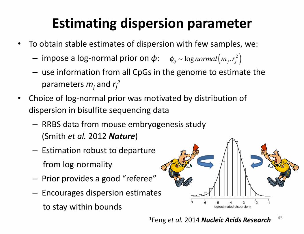
• Toobtainstableestimatesofdispersionwithfewsamples,we:– imposealog-normalprioronϕ:– useinformationfromallCpGs inthegenometoestimatethe

parametersmj andrj2

• Choiceoflog-normalpriorwasmotivatedbydistributionofdispersioninbisulfitesequencingdata– RRBSdatafrommouseembryogenesisstudy

(Smithetal.2012Nature)– Estimationrobusttodeparture

fromlog-normality– Priorprovidesagood“referee”– Encouragesdispersionestimates

tostaywithinbounds45

Smith et al. data

log(estimated dispersion)−7 −6 −5 −4 −3 −2 −1

Estimatingdispersionparameter

φij ~ lognormal mj ,rj2( )


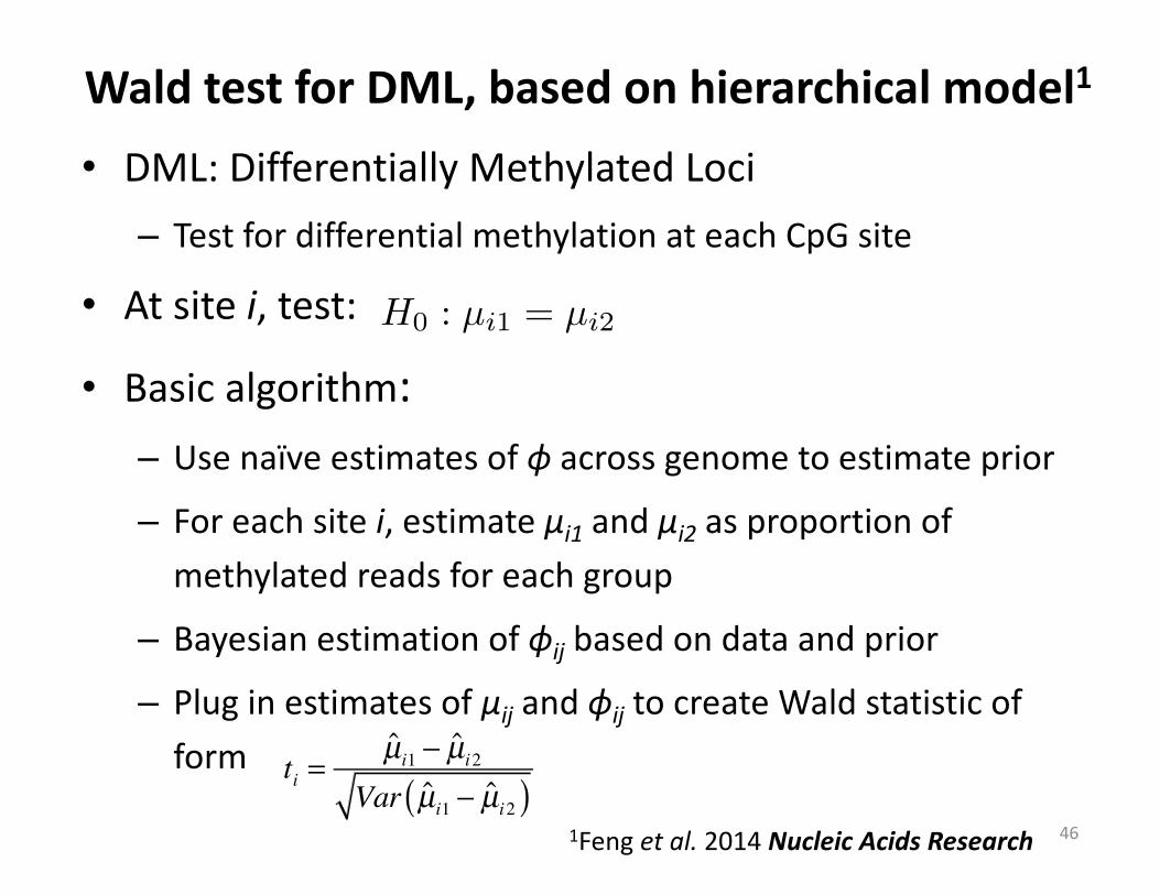
WaldtestforDML,basedonhierarchicalmodel1

• DML:DifferentiallyMethylatedLoci– TestfordifferentialmethylationateachCpG site

• Atsitei,test:

• Basicalgorithm:– Usenaïveestimatesofϕ acrossgenometoestimateprior

– Foreachsitei,estimateμi1 andμi2 asproportionofmethylatedreadsforeachgroup

– Bayesianestimationofϕij basedondataandprior

– Pluginestimatesofμij andϕij tocreateWaldstatisticofform

Xijk|Nijk, pijk ⇠ Bin(Nijk, pijk)

pijk ⇠ Beta(µik,�i)

H0 : µi1 = µi2

In beta distribution

E(X) =↵

↵+ �⌘ µ; V (X) =

↵�

(↵+ �)2(↵+ � + 1)⌘ �

2

�2 = µ ⇤ (1� µ) ⇤ 1

↵+�+1

� ⌘ 1↵+�+1

In beta-binomial

E(X) =N↵

↵�⌘ Nµ

V (X) =N↵�(↵+ � +N)

(↵+ �)2(↵+ � + 1)⌘ �

2

�2 = Nµ ⇤ (1� µ)⇤

1

46

ti =µi1 − µi2

Var µi1 − µi2( )1Fengetal.2014NucleicAcidsResearch

UsingDSS tocallDMLandDMRs• DSScanidentifydifferentiallymethylatedloci (DML)andregions (DMRs)– DMLidentifiedviaWaldtest,basedonp-valuethreshold– DMRscalledfromDMLbasedonuser-specifiedcriteria(regionlength,p-valueandeffectsizethresholds)

• NewfeaturesinDSS– Accommodatessingle-replicatestudiesbysmoothingdatafromnearbyCpG sitestoform“pseudo-replicates”1

– Inclusionofdesignmatrixtoallowcovariatesandamoregeneralexperimentaldesign2

47

1Wuetal.NucleicAcidsResearch2015.2Parketal.Bioinformatics 2016.

BS-seqexperimentundergeneraldesign

• Generalexperimentaldesign:– Multiplegroups.– Multiplefactors,crossed/nested.– Continuouscovariates.

• Limiteddataanalysismethodswithnotsogoodproperties:– BiSeq andRADMeth,bothbasedongeneralizedlinearmodel(GLM).

– Computationallydemanding.– Numericallyunstable.

DSS-general

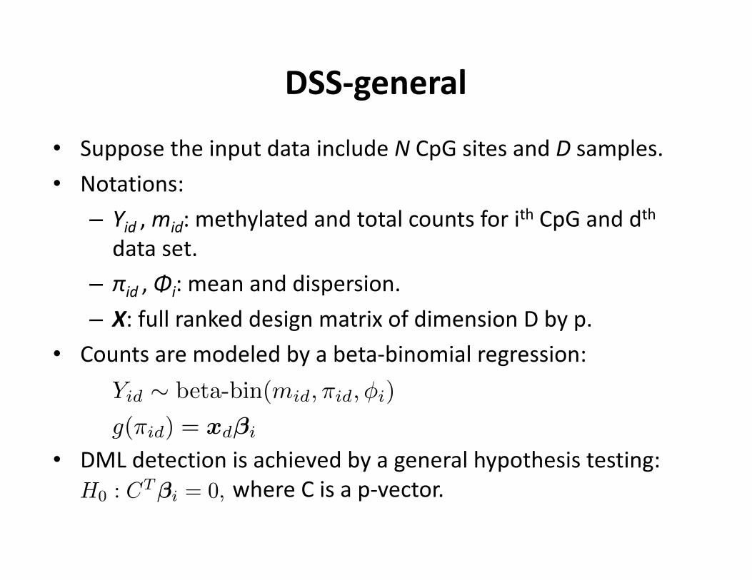
• SupposetheinputdataincludeN CpGsitesandD samples.• Notations:

– Yid,mid:methylatedandtotalcountsforith CpGanddthdataset.

– πid,Φi:meananddispersion.– X:fullrankeddesignmatrixofdimensionDbyp.

• Countsaremodeledbyabeta-binomialregression:

• DMLdetectionisachievedbyageneralhypothesistesting:whereCisap-vector.

This is for slides

Yid ⇠ beta-bin(mid,⇡id,�i)

g(⇡id) = xd�i

1

This is for slides


g(⇡id) = xd�i

H0 : CT�i = 0, where C is a p-vector.

1

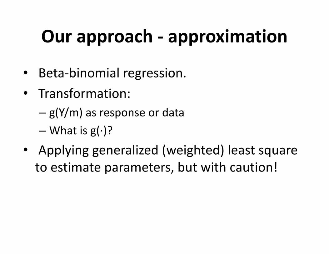
Ourapproach- approximation

• Beta-binomialregression.• Transformation:– g(Y/m)asresponseordata–Whatisg(·)?

• Applyinggeneralized(weighted)leastsquaretoestimateparameters,butwithcaution!

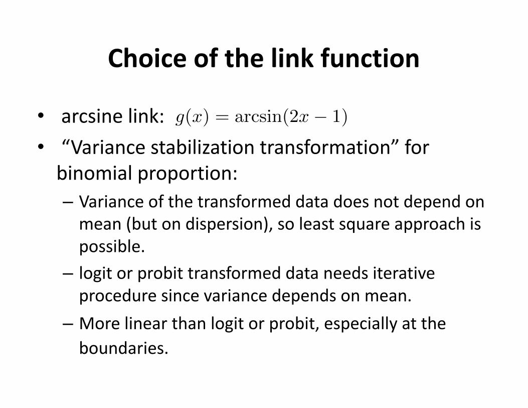
Choiceofthelinkfunction

• arcsinelink:• “Variancestabilizationtransformation”forbinomialproportion:– Varianceofthetransformeddatadoesnotdependonmean(butondispersion),soleastsquareapproachispossible.

– logitorprobit transformeddataneedsiterativeproceduresincevariancedependsonmean.

– Morelinearthanlogit orprobit,especiallyattheboundaries.

This is for slides


g(⇡id) = xd�i


g(x) = arcsin(2x� 1).

1

Parameterestimation

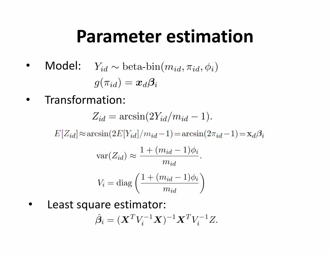
Considering a transformation Zid = arcsin(2Yid/mid � 1). We have:

E[Zid] ⇡ arcsin(2E[Yid]/mid � 1) = arcsin(2⇡id � 1) = xd�i.

The variance of Zid can be obtained as follows (refer to Supplementary Materials for more details)

var(Zid) ⇡1 + (mid � 1)�i

mid. (2)

Given dispersion parameter �i, a GLS method can be applied to estimate the regression

coe�cients �i. To be specific, define the following covariance matrix:

Vi = diag

✓1 + (mid � 1)�i

mid

◆,

then

�i = (XTV

�1i X)�1XT

V�1i Z.

For beta-binomial model, there are several ways to estimate dispersion parameter such as

maximizing likelihood, and using Pearson �2 or deviance statistics. Here we propose to use

Pearson �2 statistics based on transformed linear model to estimate �i because it is less

computationally demanding and has relatively good property. We first let �i = 0 and the initial

covariance matrix is Vi0 = diag(1/mid). Then the parameter estimator from GLS with covariance

matrix V0 is: �(0)i = (XT

V�1i0 X)�1XT

V�1i0 Z.

Consider Pearson chi-square statistics �2i =

Pdmid(Zid � xd�0

i )2. Let �2

i = �2i /(D � p), an

estimator for �i is obtained as below (detailed derivations provided in Supplementary Materials):

�i =D(�2

i � 1)Pd(mid � 1)

. (3)

Note that our model is based on beta-binomial distribution and hence 0 < �i < 1, which requires

1 < �2i <

Pd(mid�1)

D + 1. However, because of random variation and approximation bias, it is

possible that �2i does not satisfy the constraints. To avoid this, we take an ad hoc procedure to

force �i to be bounded by 0.001 and 0.999. This procedure achieves some “shrinkage” e↵ects,

which helps stabilize the result.

Given estimated dispersion, the estimate of variance structure is

Vi = diag

1 + (mid � 1)�i

mid

!.

18





mid. (2)



Vi = diag

✓1 + (mid � 1)�i

mid

◆,

then

�i = (XTV

�1i X)�1XT

V�1i Z.







V�1i0 X)�1XT

V�1i0 Z.



i )2. Let �2

i = �2i /(D � p), an


�i =D(�2

i � 1)Pd(mid � 1)

. (3)


1 < �2i <

Pd(mid�1)






Vi = diag

1 + (mid � 1)�i

mid

!.

18





mid. (2)



Vi = diag

✓1 + (mid � 1)�i

mid

◆,

then

�i = (XTV

�1i X)�1XT

V�1i Z.







V�1i0 X)�1XT

V�1i0 Z.



i )2. Let �2

i = �2i /(D � p), an


�i =D(�2

i � 1)Pd(mid � 1)

. (3)


1 < �2i <

Pd(mid�1)






Vi = diag

1 + (mid � 1)�i

mid

!.

18





mid. (2)



Vi = diag

✓1 + (mid � 1)�i

mid

◆,

then

�i = (XTV

�1i X)�1XT

V�1i Z.







V�1i0 X)�1XT

V�1i0 Z.



i )2. Let �2

i = �2i /(D � p), an


�i =D(�2

i � 1)Pd(mid � 1)

. (3)


1 < �2i <

Pd(mid�1)






Vi = diag

1 + (mid � 1)�i

mid

!.

18

This is for slides


g(⇡id) = xd�i

1

• Model:

• Transformation:

• Leastsquareestimator:

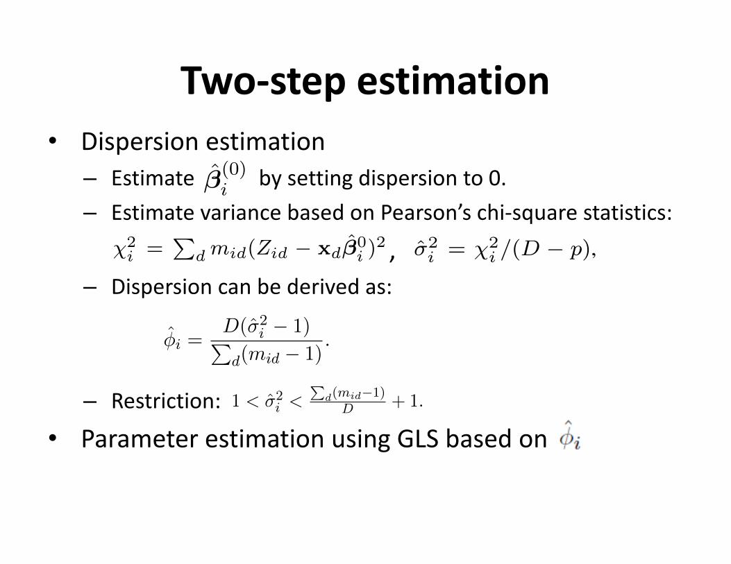
Two-stepestimation• Dispersionestimation

– Estimatebysettingdispersionto0.– EstimatevariancebasedonPearson’schi-squarestatistics:

,– Dispersioncanbederivedas:

– Restriction:

• ParameterestimationusingGLSbasedon





mid. (2)



Vi = diag

✓1 + (mid � 1)�i

mid

◆,

then

�i = (XTV

�1i X)�1XT

V�1i Z.







V�1i0 X)�1XT

V�1i0 Z.



i )2. Let �2

i = �2i /(D � p), an


�i =D(�2

i � 1)Pd(mid � 1)

. (3)


1 < �2i <

Pd(mid�1)






Vi = diag

1 + (mid � 1)�i

mid

!.

18





mid. (2)



Vi = diag

✓1 + (mid � 1)�i

mid

◆,

then

�i = (XTV

�1i X)�1XT

V�1i Z.







V�1i0 X)�1XT

V�1i0 Z.



i )2. Let �2

i = �2i /(D � p), an


�i =D(�2

i � 1)Pd(mid � 1)

. (3)


1 < �2i <

Pd(mid�1)






Vi = diag

1 + (mid � 1)�i

mid

!.

18





mid. (2)



Vi = diag

✓1 + (mid � 1)�i

mid

◆,

then

�i = (XTV

�1i X)�1XT

V�1i Z.







V�1i0 X)�1XT

V�1i0 Z.



i )2. Let �2

i = �2i /(D � p), an


�i =D(�2

i � 1)Pd(mid � 1)

. (3)


1 < �2i <

Pd(mid�1)






Vi = diag

1 + (mid � 1)�i

mid

!.

18

DSS-general

then�i = (XTV �1

i X)�1XTV �1i Z.

For beta-binomial model, there are several ways to estimate dispersionparameter such as maximizing likelihood, and using Pearson �

2 or deviancestatistics. Here we propose to use Pearson �

2 statistics based on transformedlinear model to estimate �i because it is less computationally demanding andhas relatively good property. We first let �i = 0 and the initial covariancematrix is Vi0 = diag(1/mid). The parameter estimator from GLS withcovariance matrix Vi0 is: �(0)

i = (XTV �1i0 X)�1XTV �1

i0 Z.


Pd mid(Zid � xd�0

i )2.

Let �2i = �

2i /(D � p), an estimator for �i is obtained as below (detailed

derivations provided in Supplementary Materials):

�i =D(�2

i � 1)P

d(mid � 1). (3)

Our model is based on beta-binomial distribution and hence 0 < �i < 1,which requires 1 < �

2i <

Pd(mid�1)

D + 1. However, because of randomvariation and approximation bias, it is possible that �2

i does not satisfy theconstraints. To avoid this, we restrict �i to be bounded by 0.001 and 0.999.

Given estimated dispersion, the estimate of variance structure is now

Vi = diag

1 + (mid � 1)�i

mid

!.

GLS procedure is applied once more based on Vi, and the updated estimatesfor regression coefficients and covariance matrix are obtained as

�i = (XT V �1i X)�1XT V �1

i Z,

and⌃i ⌘ \var(�i) = (XT V �1

i X)�1.

The estimation procedure utilizes two GLS for each CpG site withoutrelying on intensive iterative algorithm. It has profound connection witha beta-binomial GLM, in which the initial regression coefficients areestimated from logistic regression and using Pearson �

2 statistics to estimatedispersion parameter similar to equation (3) (Hinde and Demetrio, 1998).The covariance structure Vi is diagonal matrix. Thus our GLS procedure isalso a wighted least square, where weight for sample d is V �1/2

id .

2.4 Hypothesis testing

Hypothesis testing for differential methylation at CpG site i can beformulated as: H0 : CT�i = 0. Here C is a p-vector. The procedure isvery general and can test any linear combination of the effects. For example,to test the effect of factor k, C will be a vector having 1 at the k

th elementand 0’s in all others. With point estimation and estimated covariance matrix,the null hypothesis is tested through a standard Wald test procedure. TheWald test statistics is calculated as:

ti =CT �iqCT ⌃iC

.

The Wald test statistics approximately follow normal distribution, andthe p-values can be obtained accordingly. False discovery rate (FDR) willbe estimated using established procedures such as Benjamini-Hochberg’smethod (Benjamini and Hochberg, 1995).

2.5 Simulation settings

In all simulations, data are generated semi-parametrically. The countsare generated from the data model described in Equation (1) with modelparameters estimated from the human lung adenocarcinoma dataset. Themodel is 2 ⇥ 2 factorial design with 20,000 CpG sites for 3 replicatesin each condition group (12 datasets in total). For each factor, 5% of theCpG sites are DML, and the DM status for two factors are independentlygenerated. The regression coefficients �g (g = 0, 1, 2) are simulated in

the following way: (1) �0 (the intercept) is randomly sampled from theestimated intercepts from real data; (2) �1 and �2 are set to be 0 if the CpGsite is not DML, and sampled from N(0, 1) if the CpG site is DML; (3)The dispersion parameter �i’s are independently generated from log-normaldistribution with mean -3 and standard deviation 0.7, which are similar tothe real data estimates.

We also perform simulations when data are generated from a GLM with“logit” link to assess the robustness of our method. In this case, since thescales of the coefficients under “logit” link are greater than those from“arcsine” link for the same data (by a ratio of approximately 2.3), wemultiply 2.3 for �g’s for all simulations using “logit” link.

3 RESULTS3.1 Simulation

Comprehensive simulation studies are conducted to evaluate theperformance of DSS-general from several different aspects.

3.1.1 Dispersion estimation Dispersion parameter is an importantcomponent in various types of differential analysis for sequencingdata. Improved dispersion estimation from RNA-seq and BS-seqin two-group comparison has been shown to lead to better resultsin differential expression and differential methylation analyses(Robinson and Smyth, 2007; Wu et al., 2013; Feng et al., 2014;Love et al., 2014).

The estimated dispersions from DSS-general are compared tothe true ones in this simulation. Overall, the Pearson correlationbetween estimated and true dispersions is moderate at around 0.4.Data exploration indicates that large differences of estimated andtrue dispersions are mostly comes from the following two types ofCpG sites: (1) those with average methylation levels very close to0 or 1 and (2) those with low sequencing depth. For those CpGsites, it is not surprising to see estimates with large variation dueto low in-data information. The correlation indeed improves to 0.55when restricted to those with average methylation levels between0.3 and 0.7, and to 0.74 when further restricted to those with averagesequencing depth of at least 30. Figure ?? shows a plot for estimatedvs true dispersions for CpG sites with methylation levels between0.3 and 0.7. Sites with different levels of sequencing depth arerepresented by different colors. It shows reasonably good dispersionestimation.

3.1.2 DML detection accuracy We next compare the DMLdetection accuracies from several methods, including DSS-general,RADMeth, BiSeq and a binomial GLM with “logit” link incomparison. Here, the proportion of true positives among a givennumber of top-ranked CpGs is used as criterion. This refers to truediscovery rate (TDR) hereafter. Higher TDR is expected from bettermethod. This criterion is also referred to precision–recall analysis.Because the proportion of true positives is usually very low in DManalysis (5% in simulation setting), TDR is a better measurementof the accuracy for genome-wide differential analysis than receiveroperating characteristic (ROC) (Davis and Goadrich, 2006).

Each simulation is repeated 50 times to obtain the averageTDR estimates. Figure 1(A) shows the TDR curves up to top1,000 (5% of total) CpG sites when data are simulated using“arcsine” link function. It can be seen that DSS-general outperformsother methods for all top ranked CpG sites. For example, amongtop 200 ranked CpGs from DSS-general, 99.8% are true DML,whereas the percentages are 93.6%, 82.4%, and 38.4% from

3

DSS-general

then�i = (XTV �1

i X)�1XTV �1i Z.

For beta-binomial model, there are several ways to estimate dispersionparameter such as maximizing likelihood, and using Pearson �

2 or deviancestatistics. Here we propose to use Pearson �

2 statistics based on transformedlinear model to estimate �i because it is less computationally demanding andhas relatively good property. We first let �i = 0 and the initial covariancematrix is Vi0 = diag(1/mid). The parameter estimator from GLS withcovariance matrix Vi0 is: �(0)

i = (XTV �1i0 X)�1XTV �1

i0 Z.


Pd mid(Zid � xd�0

i )2.

Let �2i = �

2i /(D � p), an estimator for �i is obtained as below (detailed

derivations provided in Supplementary Materials):

�i =D(�2

i � 1)P

d(mid � 1). (3)

Our model is based on beta-binomial distribution and hence 0 < �i < 1,which requires 1 < �

2i <

Pd(mid�1)

D + 1. However, because of randomvariation and approximation bias, it is possible that �2

i does not satisfy theconstraints. To avoid this, we restrict �i to be bounded by 0.001 and 0.999.

Given estimated dispersion, the estimate of variance structure is now

Vi = diag

1 + (mid � 1)�i

mid

!.

GLS procedure is applied once more based on Vi, and the updated estimatesfor regression coefficients and covariance matrix are obtained as

�i = (XT V �1i X)�1XT V �1

i Z,

and⌃i ⌘ \var(�i) = (XT V �1

i X)�1.

The estimation procedure utilizes two GLS for each CpG site withoutrelying on intensive iterative algorithm. It has profound connection witha beta-binomial GLM, in which the initial regression coefficients areestimated from logistic regression and using Pearson �

2 statistics to estimatedispersion parameter similar to equation (3) (Hinde and Demetrio, 1998).The covariance structure Vi is diagonal matrix. Thus our GLS procedure isalso a wighted least square, where weight for sample d is V �1/2

id .

2.4 Hypothesis testing

Hypothesis testing for differential methylation at CpG site i can beformulated as: H0 : CT�i = 0. Here C is a p-vector. The procedure isvery general and can test any linear combination of the effects. For example,to test the effect of factor k, C will be a vector having 1 at the k

th elementand 0’s in all others. With point estimation and estimated covariance matrix,the null hypothesis is tested through a standard Wald test procedure. TheWald test statistics is calculated as:

ti =CT �iqCT ⌃iC

.

The Wald test statistics approximately follow normal distribution, andthe p-values can be obtained accordingly. False discovery rate (FDR) willbe estimated using established procedures such as Benjamini-Hochberg’smethod (Benjamini and Hochberg, 1995).


In all simulations, data are generated semi-parametrically. The countsare generated from the data model described in Equation (1) with modelparameters estimated from the human lung adenocarcinoma dataset. Themodel is 2 ⇥ 2 factorial design with 20,000 CpG sites for 3 replicatesin each condition group (12 datasets in total). For each factor, 5% of theCpG sites are DML, and the DM status for two factors are independentlygenerated. The regression coefficients �g (g = 0, 1, 2) are simulated in

the following way: (1) �0 (the intercept) is randomly sampled from theestimated intercepts from real data; (2) �1 and �2 are set to be 0 if the CpGsite is not DML, and sampled from N(0, 1) if the CpG site is DML; (3)The dispersion parameter �i’s are independently generated from log-normaldistribution with mean -3 and standard deviation 0.7, which are similar tothe real data estimates.

We also perform simulations when data are generated from a GLM with“logit” link to assess the robustness of our method. In this case, since thescales of the coefficients under “logit” link are greater than those from“arcsine” link for the same data (by a ratio of approximately 2.3), wemultiply 2.3 for �g’s for all simulations using “logit” link.

3 RESULTS3.1 Simulation

Comprehensive simulation studies are conducted to evaluate theperformance of DSS-general from several different aspects.

3.1.1 Dispersion estimation Dispersion parameter is an importantcomponent in various types of differential analysis for sequencingdata. Improved dispersion estimation from RNA-seq and BS-seqin two-group comparison has been shown to lead to better resultsin differential expression and differential methylation analyses(Robinson and Smyth, 2007; Wu et al., 2013; Feng et al., 2014;Love et al., 2014).

The estimated dispersions from DSS-general are compared tothe true ones in this simulation. Overall, the Pearson correlationbetween estimated and true dispersions is moderate at around 0.4.Data exploration indicates that large differences of estimated andtrue dispersions are mostly comes from the following two types ofCpG sites: (1) those with average methylation levels very close to0 or 1 and (2) those with low sequencing depth. For those CpGsites, it is not surprising to see estimates with large variation dueto low in-data information. The correlation indeed improves to 0.55when restricted to those with average methylation levels between0.3 and 0.7, and to 0.74 when further restricted to those with averagesequencing depth of at least 30. Figure ?? shows a plot for estimatedvs true dispersions for CpG sites with methylation levels between0.3 and 0.7. Sites with different levels of sequencing depth arerepresented by different colors. It shows reasonably good dispersionestimation.

3.1.2 DML detection accuracy We next compare the DMLdetection accuracies from several methods, including DSS-general,RADMeth, BiSeq and a binomial GLM with “logit” link incomparison. Here, the proportion of true positives among a givennumber of top-ranked CpGs is used as criterion. This refers to truediscovery rate (TDR) hereafter. Higher TDR is expected from bettermethod. This criterion is also referred to precision–recall analysis.Because the proportion of true positives is usually very low in DManalysis (5% in simulation setting), TDR is a better measurementof the accuracy for genome-wide differential analysis than receiveroperating characteristic (ROC) (Davis and Goadrich, 2006).

Each simulation is repeated 50 times to obtain the averageTDR estimates. Figure 1(A) shows the TDR curves up to top1,000 (5% of total) CpG sites when data are simulated using“arcsine” link function. It can be seen that DSS-general outperformsother methods for all top ranked CpG sites. For example, amongtop 200 ranked CpGs from DSS-general, 99.8% are true DML,whereas the percentages are 93.6%, 82.4%, and 38.4% from

3

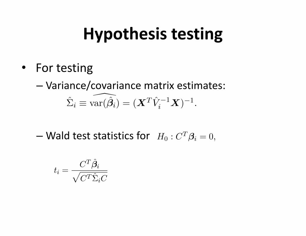
Hypothesistesting

• Fortesting– Variance/covariancematrixestimates:

–Waldteststatisticsfor

This is for slides


g(⇡id) = xd�i


1

Then the coe�cient estimate is: �i = (XTV

�1i X)�1XT

V�1i Z, and the estimated covariance

matrix of the parameter estimates is ⌃i ⌘ \var(�i) = (XTV

�1i X)�1.

This estimation procedure utilizes two GLS estimations for each CpG site, which is

computationally very e�cient without relying on any iterative algorithm. The above procedure

has profound connection with a beta-binomial GLM, in which the initial regression coe�cients are

estimated from logistic regression and using Pearson �2 statistics to estimate dispersion

parameter in the similar way as equation (3) [44].

4.3.1 Hypothesis testing

Hypothesis testing for di↵erential methylation at CpG site i can be formulated as: H0 : CT�i = 0.

Here C is a p-vector. The procedure is very general and can test any linear combination of the

e↵ects. For example, to test the e↵ect of factor k, C will be a vector having 1 at the kth element

and 0’s in all others. With point estimates and estimated covariance matrix, the null hypothesis

is tested through a standard Wald test procedure. The Wald test statistics is calculated as:

ti =C

T �ipCT ⌃iC

The Wald test statistics approximately follow normal distribution, so that the p-values can be

obtained accordingly. False discovery rate (FDR) will be estimated using established procedures

such as Benjamini-Hochberg’s method [45].


For all simulations, the data are generated semi-parametrically, i.e., the counts are generated from

the data model described in Equation (1) with model parameters estimated from the human lung

adenocarcinoma dataset. In all simulations, data are generated for a 2⇥ 2 factorial design, with

20,000 CpG sites and 3 replicates in each condition (12 datasets in total). For each factor, we

assume 5% of the CpG sites are DML, and the DM status for two factors are independent. The

regression coe�cients �g (g = 0, 1, 2) are simulated in the following way. �0 (the intercept) is

randomly sampled from the estimated intercept of real data. �1 and �2 are set to be 0 if the CpG

19

Then the coe�cient estimate is: �i = (XTV

�1i X)�1XT

V�1i Z, and the estimated covariance

matrix of the parameter estimates is ⌃i ⌘ \var(�i) = (XTV

�1i X)�1.

This estimation procedure utilizes two GLS estimations for each CpG site, which is

computationally very e�cient without relying on any iterative algorithm. The above procedure

has profound connection with a beta-binomial GLM, in which the initial regression coe�cients are

estimated from logistic regression and using Pearson �2 statistics to estimate dispersion

parameter in the similar way as equation (3) [44].

4.3.1 Hypothesis testing

Hypothesis testing for di↵erential methylation at CpG site i can be formulated as: H0 : CT�i = 0.

Here C is a p-vector. The procedure is very general and can test any linear combination of the

e↵ects. For example, to test the e↵ect of factor k, C will be a vector having 1 at the kth element

and 0’s in all others. With point estimates and estimated covariance matrix, the null hypothesis

is tested through a standard Wald test procedure. The Wald test statistics is calculated as:

ti =C

T �ipCT ⌃iC

The Wald test statistics approximately follow normal distribution, so that the p-values can be

obtained accordingly. False discovery rate (FDR) will be estimated using established procedures

such as Benjamini-Hochberg’s method [45].


For all simulations, the data are generated semi-parametrically, i.e., the counts are generated from

the data model described in Equation (1) with model parameters estimated from the human lung

adenocarcinoma dataset. In all simulations, data are generated for a 2⇥ 2 factorial design, with

20,000 CpG sites and 3 replicates in each condition (12 datasets in total). For each factor, we

assume 5% of the CpG sites are DML, and the DM status for two factors are independent. The

regression coe�cients �g (g = 0, 1, 2) are simulated in the following way. �0 (the intercept) is

randomly sampled from the estimated intercept of real data. �1 and �2 are set to be 0 if the CpG

19

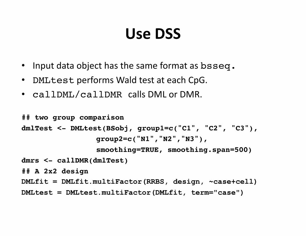
UseDSS

• Inputdataobjecthasthesameformatasbsseq.• DMLtest performsWaldtestateachCpG.• callDML/callDMR callsDMLorDMR.

## two group comparisondmlTest <- DMLtest(BSobj, group1=c("C1", "C2", "C3"),

group2=c("N1","N2","N3"),smoothing=TRUE, smoothing.span=500)

dmrs <- callDMR(dmlTest)## A 2x2 designDMLfit = DMLfit.multiFactor(RRBS, design, ~case+cell) DMLtest = DMLtest.multiFactor(DMLfit, term="case")

Conclusions• Analysisofgenome-widebisulfitesequencingdatapresentssomeuniquechallenges– Alignmentofreadscanbecomplicated– Manyteststobeperformed,butnumberofsamplessequencedislimitedbycostsinmostexperiments

– Beta-binomialmodeliswidelyused.

56

Forsoftware/analysis• Akalin etal.2012GenomeBiology13:R87.MethylKit paper.• Chatterjee etal.(2012)NucleicAcidsResearch.40(10):e79.Comparesaligners.• Chavezetal.(2010)GenomeResearch20:1441-50.MEDIPSsoftware.• Dolzhenko andSmith(2014)BMCBioinformatics 15:215.RADMeth.• Feng,Conneely,andWu(2014)NucleicAcidsResearch42(8):e69,DSSfortwo-group.• Hansenetal.(2012)GenomeBiology 13:R83. Bsmooth paper.• Hebestreit,Dugas,andKlein(2013)Bioinformatics 29:1647-53.BiSeq.• KruegerandAndrews(2011)Bioinformatics27(11):1571-2.BISMARKaligner.• Parketal.(2014)Bioinformatics 30:2414-22.MethylSig.• Robinsonetal.(2014)FrontiersinGenetics5:324.ReviewofmethodsforDMLandDMR• Stadler etal.(2012)Nature480:490-6.Mousemethylome paperthatusedHMM.• Sunetal.(2014)GenomeBiology 15:R38.MOABS.• Wuetal.(2015)NucleicAcidsResearch.43(21):e141.DSS-singleforsinglereplicates.• ParkandWu(2016)Bioinformatics32(10),1446-1453. DSS-generalforgeneraldesign.• XiandLi(2009)BMCBioinformatics 10:232.BSMAPaligner.• Xietal.(2012)Bioinformatics 28(3):430-2.RRBSMAPaligner.

57

References

Fordifferentsequencingtechnologies• Bocketal.(2010)NatBiotech 28(10):1106-16.ComparesRRBS,MeDIP-seq,others• Brinkmanetal.(2010)Methods52:232-236.MethylCap-seq.• Gu etal.(2011)NatProtoc 6(4):468-81.Genome-wideRRBSprotocol.• Maunakea etal.(2010)Nature466:253-7.MRE-seq.• Meissner (2005)NucleicAcidsResearch.33:5868-77.OriginalRRBSpaper.• Rauchetal.(2010)Methods52:213-7.MIRA-seq.• Serre etal.(2010)NucleicAcidsResearch.38:391-9.MBD-seq.• Weberetal.(2005)NatGenet 37:853-62.OriginalMeDIP paper.

58

References

bisulfite sequencing - haowulab.org · varleyk e et al. genome res. 2013;23:555-567 in human...

Documents