bis working papers · samuelson effect for these countries is therefore of particular interest....

BIS Working Papers No 270

Catching-up and inflation in transition economies: the Balassa-Samuelson effect revisited by Dubravko Mihaljek and Marc Klau

Monetary and Economic Department

December 2008

JEL codes: E31, F36, O11, P20

Keywords: Balassa-Samuelson effect, productivity, inflation, transition, convergence, European monetary union, Maastricht criteria

BIS Working Papers are written by members of the Monetary and Economic Department of the Bank for International Settlements, and from time to time by other economists, and are published by the Bank. The views expressed in them are those of their authors and not necessarily the views of the BIS.

Copies of publications are available from:

Bank for International Settlements Press & Communications CH-4002 Basel, Switzerland E-mail: [email protected]

Fax: +41 61 280 9100 and +41 61 280 8100

This publication is available on the BIS website (www.bis.org).

© Bank for International Settlements 2008. All rights reserved. Limited extracts may be reproduced

or translated provided the source is stated.

ISSN 1020-0959 (print)

ISSN 1682-7678 (online)

mailto:[email protected]

http://www.bis.org/

Catching-up and inflation in transition economies: the Balassa-Samuelson effect revisited

Dubravko Mihaljek and Marc Klau1

Abstract

This paper estimates the Balassa-Samuelson effects for 11 countries in central and eastern Europe on a disaggregated set of quarterly data covering the period from the mid-1990s to the first quarter of 2008. The Balassa-Samuelson effects are clearly present and explain around 24% of inflation differentials vis-à-vis the euro area (about 1.2 percentage points on average); and around 84% of domestic relative price differentials between non-tradables and tradables; or about 16% of total domestic inflation (about 1.1 percentage points on average). The paper presents mixed evidence on whether the Balassa-Samuelson effects have declined since 2001 compared with the second half of the 1990s.

JEL Classification Numbers: E31, F36, O11, P20

Keywords: Balassa-Samuelson effect, productivity, inflation, transition, convergence, European monetary union, Maastricht criteria

1 Senior Economist and Head of Departmental Research Assistance, respectively, Monetary and Economic

Department, Bank for International Settlements, CH-4002 Basel, Switzerland. Corresponding author: [email protected] The views expressed in this paper are those of the authors and do not necessarily represent those of the BIS. Helpful comments from Claudio Borio, Lina Bukeviciute, Andy Filardo, Roman Horvath, Richhild Moessner and participants of a BIS seminar and the European Commission DG ECFIN workshop “What drives inflation in the new EU member states?” (October 2008) are gratefully acknowledged.

Catching-up and inflation in transition economies 1

mailto:[email protected]

1. Introduction

The purpose of this paper is to assess, as precisely and transparently as possible, the degree to which faster productivity growth in tradable versus non-tradable sectors of countries in central and eastern Europe (CEE) contributes to domestic inflation and to inflation differentials that these countries exhibit vis-à-vis the euro area. These two effects – the domestic and international versions of the Balassa-Samuelson effect – are part of the structural inflation phenomenon and as such are of key importance for economic policy. As observed by Padoa-Schioppa (2003), not all inflation in the catching-up economies is “pathological” – faster productivity growth in industries producing tradable goods and services is part of the “physiology” of economic development. If labour and capital markets are unencumbered, there is not much that economic policy could or should do to control this source of inflation.

The magnitude of the Balassa-Samuelson effect is therefore of considerable interest for policymakers in EMU candidate countries and relevant EU institutions. If the productivity growth differential between the traded and non-traded goods sectors is larger in an EMU candidate country than the euro area, the overall inflation will be higher in the candidate country. Under a fixed exchange rate regime, this will result in real exchange rate appreciation. Under a flexible exchange rate regime, it will result in some combination of nominal appreciation and CPI inflation. Both scenarios might create problems with the fulfilment of the Maastricht criteria for inflation and exchange rate stability.

Consider countries with a fixed exchange rate regime. If monetary policy were to keep inflation around the benchmark – average of three EU countries with lowest inflation – but the Balassa-Samuelson effect was greater than the 1½ percentage point margin allowed by the Maastricht treaty, the inflation criterion might be missed.2 The authorities might therefore feel compelled to maintain, at least temporarily, relatively restrictive monetary and fiscal policies in order to meet the inflation criterion. This might dampen economic growth and job creation. In such circumstances, it might be difficult to explain to the public why the economy needs to slow down in order to adopt the common currency – reasonable observers might argue that the country is being “punished” for catching up too fast.

In countries with flexible exchange rate regimes, the policy dilemma resulting from the Balassa-Samuelson effect is somewhat less pronounced. If monetary policy were to keep inflation below the Maastricht ceiling but the Balassa-Samuelson effect was greater than 1½ percentage points, the optimal response would be to allow the exchange rate to appreciate. The resulting appreciation is not likely to be a major obstacle for the fulfilment of the exchange rate stability criterion: the Balassa-Samuelson effect would have to be truly large to exhaust the 15% band of the ERM II in two years, assuming that the exchange rate starts in the middle of the band.3 However, rapid exchange rate appreciation might attract

2 According to the Maastricht inflation criterion, EMU candidates have to show a price stability performance that

is sustainable and an average rate of inflation (observed over a period of one year before the examination) that does not exceed by more than 1½ percentage points that of, at most, the three EU member states with the best price stability performance.

3 The Maastricht exchange rate stability criterion requires EMU candidates to spend at least two years “without severe tensions” – in particular without devaluing against the euro – in the exchange rate mechanism of the European Monetary System, the so-called ERM II. ERM II is an exchange rate arrangement with fixed but adjustable central parities against the euro and a normal fluctuation band of ±15% around these parities. The assessment of exchange rate stability against the euro focuses on the exchange rate being close to the central rate while also taking into account factors that may have led to an appreciation. The width of the fluctuation band within ERM II does not prejudice the assessment of the exchange rate stability criterion.

2 Catching-up and inflation in transition economies

large and volatile capital inflows and through this channel negatively affect financial stability and external competitiveness (see Mihaljek, 2008).

Not surprisingly, there has been much discussion in the literature on the existence, size and policy implications of the Balassa-Samuelson effect in CEE, so much so that the first literature reviews have been published (see eg Égert, 2003; Égert et al, 2006). The early empirical literature (Golinelli and Orsi, 2002; Halpern and Wyplosz, 2001; Kovács and Simon, 1998; Rother, 2000) argued that the Balassa-Samuelson effect was relatively large. If inflation is structurally out of line with the benchmark value in the EU because of strong catching-up effects, the proposition to relax the inflation criterion becomes empirically plausible. Consequently, there have been calls both by academics (Begg et al, 2003; Buiter and Grafe, 2002; Buiter and Siebert, 2006; Darvas and Szapáry, 2008) and policy makers (Szapáry, 2000) to relax the Maastricht inflation criterion.4

However, more recent empirical studies found the Balassa-Samuelson effect to be relatively small. For instance, in our earlier paper (Mihaljek and Klau, 2004) we found that the Balassa-Samuelson effect in central European countries explained on average only between 0.2 and 2.0 percentage points of annual inflation differentials vis-à-vis the euro area. We also argued that, as the pace of catching-up decelerates, these effects were likely to decrease and hence should not become a determining factor in the ability of these countries to satisfy the Maastricht inflation criterion. Other studies (including Cipriani, 2001; Coricelli and Jazbec, 2001; Égert, 2002a and 2002b; Égert et al, 2003; Flek et al, 2002; Kovács, 2002; Lojschova, 2003) similarly found these effects to be small.

The literature has also identified some puzzles related to the operation of the Balassa-Samuelson effect (see Égert and Podpiera, 2008). On the one hand, the evidence suggests that this effect is not the main driving force of the observed relatively high inflation rates of 3–6% per annum in most CEE countries. On the other hand, although productivity growth in the tradable sectors has indeed been high, it has not led to correspondingly high inflation rates. Several explanations of these puzzles have been elaborated, including a trend increase in tradable prices related, inter alia, to steady quality improvements (Cincibuch and Podpiera, 2006); the role of regulated price adjustments in overall inflation (MacDonald and Wojcik, 2004); a disconnection between productivity growth and real wages in the manufacturing sector (Égert, 2007); incomplete wage equalisation and substantial productivity gains in market non-tradables (Alberola-Ila and Tyrväinen, 1998); and the low share of market non-tradables in consumer price indices of CEE countries (Égert et al, 2006).

Any addition to this burgeoning literature therefore has to be justified. The main contribution of the present paper is the size and up-to-dateness of the sample – we analyse quarterly data from eleven CEE countries from the mid-1990s through the first quarter of 2008. For more than half of the countries in our sample – Bulgaria, Croatia, Estonia, Latvia, Lithuania and Romania – there are only a handful of empirical studies of the Balassa-Samuelson effect.5 For these six countries as well as the remaining new member states from CEE included in our sample – the Czech Republic, Hungary, Poland, Slovakia and Slovenia – there have been hardly any estimates of the Balassa-Samuelson effect covering the period since 2004.6 This period is relevant because, with the exception of Croatia, all countries in the sample have since joined the European Union. Several of them (including the Baltic states) have entered the exchange rate mechanism ERM II, and two of these – Slovenia and

4 For overviews, see eg Deroose and Baras (2005); and Mihaljek (2006). 5 See Burgess et al (2003); Chukalev (2002); Égert (2005a) and (2005b); Égert et al (2003); Funda et al (2007);

Mihaljek and Klau (2004) and (2007); Nenovsky and Dimitrova (2002); and Wagner and Hlouskova (2004). 6 In Mihaljek and Klau (2007) we cover the period through 2005:Q1 for six central European countries.


Slovakia – have already passed the Maastricht tests. Assessing the size of the Balassa-Samuelson effect for these countries is therefore of particular interest.

Another contribution of the present paper is greater precision of our estimates than in the past (eg, compared with Mihaljek and Klau, 2004). One reason is the much better quality of the data that have been released over the past few years by national statistical authorities and Eurostat, in particular for Poland, Slovakia, the Baltic states, Bulgaria and Romania. This has enabled us to extend the coverage of tradable sectors to agriculture, forestry and fishing, which are major sources of exports of several countries in the region; and to directly include one additional key variable, the share of non-tradables, in regression equations that are being estimated. We also examine whether productivity growth and the Balassa-Samuelson effects have diminished in recent years, an issue that has not been addressed systematically in the literature so far.

Finally, one advantage of our approach is the simple, transparent estimating framework that can be easily interpreted by policymakers and replicated by researchers with access to more disaggregated data.

Section 2 discusses the analytical framework and some relevant data issues. Section 3 reviews historical developments in productivity and inflation differentials within CEE countries and between those countries and the euro area over the sample period. Section 4 discusses our econometric estimates of the Balassa-Samuelson effects. Section 5 summarises the main results and briefly notes some of their policy implications.

2. Analytical framework

Using the distinction introduced in our 2004 paper, we discuss two versions of the Balassa-Samuelson effect, the “international” effect (equation 1) and the “domestic” effect (equation 2):7

]ˆˆ)[1(]ˆˆ)[1(ˆˆˆ ***

*** NT

tTtt

NTt

Tttttt aaaaeconstpp −⎟⎟

⎠

⎞⎜⎜⎝

⎛−−−⎟⎟

⎠

⎞⎜⎜⎝

⎛−++=−

γδα

γδα (1)

NT

t

T

t

T

t

NT

t aapp ˆˆˆˆ −⎟⎟⎠

⎞⎜⎜⎝

⎛=−

γδ

(2)

where circumflexes (^) stand for the growth rates; “*” denotes variables in the euro area; is the difference*ˆˆ tt pp − in consumer price inflation between a given CEE country and the

euro area; represents the difference in domestic inflation rates of non-tradables and tradables, ie the growth rate of the relative price of non-tradables; is the rate of nominal exchange rate depreciation (units of domestic currency vis-à-vis the euro); α

T

t

NT

t pp ˆˆ −

tet is the

share of traded goods in the consumption basket; and are the growth rates of average labour productivity in tradable and non-tradable sectors, respectively; γ and δ are production function coefficients (labour intensities in traded and non-traded sectors); and const is a term containing coefficients α, γ and δ.

Tta NT

ta

Equation (1) states that the difference in rates of inflation between two countries can be expressed as the sum of changes in the exchange rate (of the home country’s currency vis-

7 The two equations are derived in Mihaljek and Klau (2004); see also Égert (2003) and Égert et al (2006).


à-vis the foreign currency) and productivity growth differentials between traded and non-traded industries at home and abroad, weighted by the respective non-tradables’ shares.

Equation (2) states that the growth rate of the relative price of non-tradable goods can be expressed as the difference in average labour productivity growth between tradable and non-tradable sectors.

Both versions of the Balassa-Samuelson effect are thus hypotheses about the structural origins of inflation: in the international version, about the tendency for inflation in the catching-up economies to be higher than in the economies they are converging to; and in the domestic version, about the tendency for the domestic prices of non-tradables to rise faster than those of tradables.

The structural factor that explains the tendency in both cases is the relative productivity growth differential. Historically, productivity growth in the traded goods sector has been faster than in the non-traded goods sector. If the law of one price holds, the prices of tradables tend to get equalised across countries, while the prices of non-tradables do not. Higher productivity in the tradable goods sector will bid up wages in that sector and, with labour being mobile, wages in the entire economy will rise. Producers of non-tradables will be able to pay the higher wages only if the relative price of non-tradables rises. This will in general lead to an increase in overall inflation in the economy.

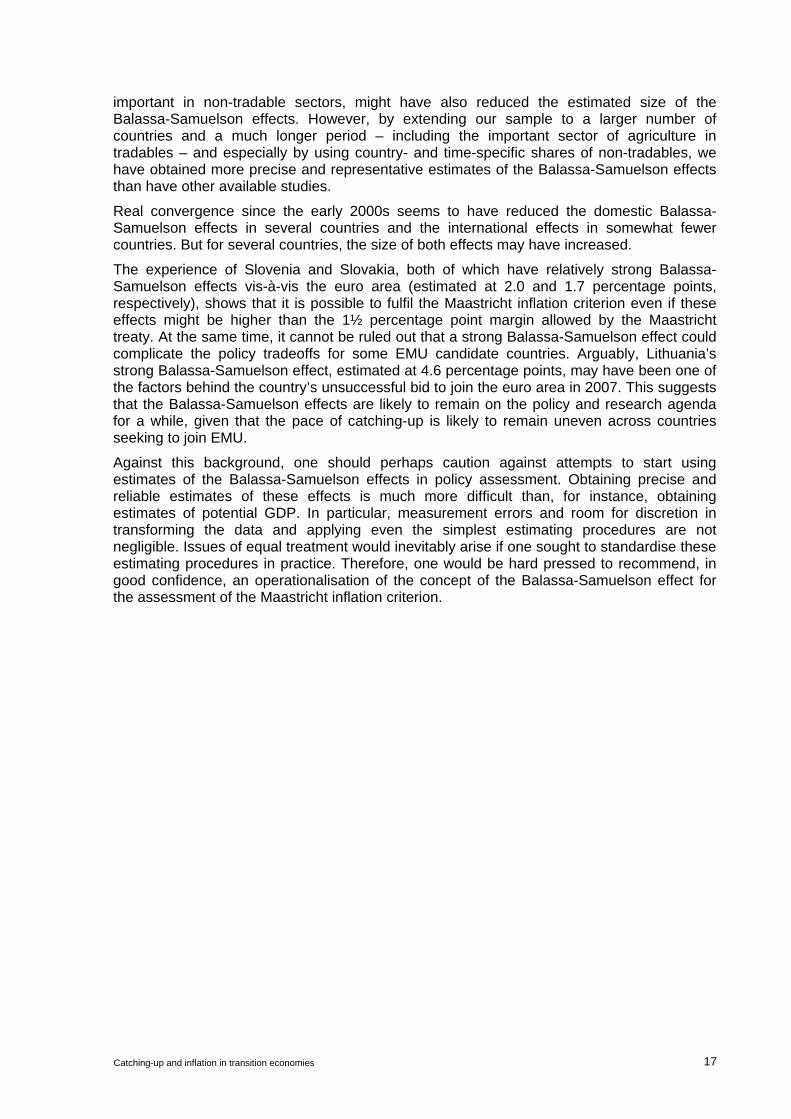
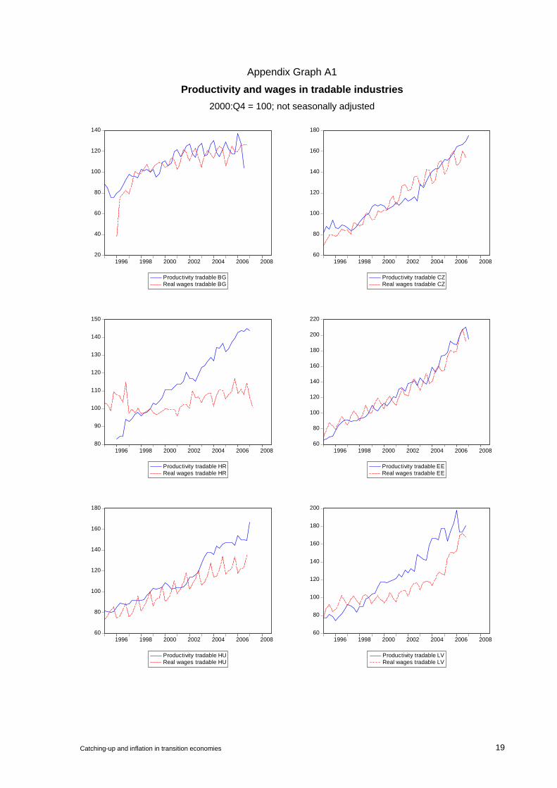
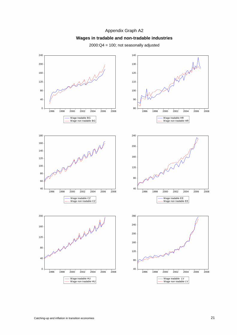
Graphs A1 and A2 in the Appendix verify two key assumptions of the Balassa-Samuelson hypothesis: first, that productivity growth in the tradable sector bids up wages in that sector; and second, that wage growth in the tradable sector spreads to the non-tradable sector. As shown in Graph A1, real wage growth in tradable industries generally closely follows productivity growth in tradables over the sample period. In some cases (Croatia, Latvia, Lithuania, Slovakia, Slovenia), strong productivity gains in tradables are not entirely passed onto real wages in that sector. Graph A2 provides clear evidence of wage equalisation between tradables and non-tradables in CEE countries – it is remarkable how closely together wages in the two sectors have moved over longer periods in virtually all the countries in the region.

Several analytical points about this model are worth noting. First, the size of the Balassa-Samuelson effect depends on the relative rather than the absolute productivity growth differential. For instance, let aT = 3%, aNT = 1%, aT* = 4%, aNT* = 3%.8 Then productivity growth in both tradables and non-tradables is higher abroad, but with (aT–aNT) > (aT*–aNT*), higher inflation at home would still be an equilibrium phenomenon. Similar to the theory of comparative advantage in international trade, the importance of the relative instead of the absolute productivity differential is often ignored in empirical studies, which assume that productivity growth in non-tradables is the same across countries or equal to zero. If this were the case, the Balassa-Samuelson effect in the above example would be negative (–1 percentage point).

Second, the size of the Balassa-Samuelson effect depends on the relative shares of non-traded goods (1–αt) at home and abroad. This is also typically ignored in empirical studies by assuming not only that αt = αt*, but also that the shares are constant over time. These assumptions, however, may lead to large overestimates of the effect.9 We avoid this bias by calculating different shares of non-traded goods for different countries for each quarterly observation in the sample. This allows a much greater precision of the estimates because

8 For ease of notation, circumflexes will be omitted in the text, graphs and tables and used only in equations. 9 For instance, data in Tables 1 and 2 imply (using the average for CEE) that (1–α)(aT–aNT) – (1–α)(aT*–aNT*) =

0.635x3.9 – 0.687x2.4 = 0.83. With α = α* = 0.635, the Balassa-Samuelson effect would be equal to 1.03, ie about 25% higher.


the shares of non-tradables range over the sample from under 40% to over 80%. On average, the non-tradables’ share in CEE increased from 58% in the mid-1990s to 69% in 2007–08.

One should also note that we derive the non-tradables’ shares from national income accounts in constant prices rather than the weight of non-tradables in consumer price indices (usually proxied by the weight of services in the CPI). While the latter is analytically correct – equation (1) is derived from the expression for the CPI as a weighted average of tradables and non-tradables – the former is preferable in empirical work because of the downward bias in the CPI weights of services in CEE countries. For instance, market-based non-tradables account for only around 20–30% of the CPI basket in the Baltic states and south-eastern Europe, although they represent on average around two-thirds of the value added in the economy. Using the CPI weights for non-tradables would therefore seriously underestimate the “true” Balassa-Samuelson effects.

Third, the Balassa-Samuelson effect is sensitive to the classification of tradable and non-tradable sectors. There is no accepted criterion for this classification, and data do not always allow one to make a clear distinction. Consider for instance an often used benchmark for tradables proposed by De Gregorio et al (1994): tradable industries are those with a share of exports in value added of 10% or more. To take an extreme example, housing is usually considered a quintessential non-tradable. But much of the housing in coastal areas of Bulgaria, Croatia and some Baltic states has been constructed and sold to non-residents in recent years. Data on such sales are generally unavailable, so a substantial part of “exports” of the construction industry might be underreported. Business services are another example of an industry typically classified as non-tradable, even though many companies in this sector are providing their services to (ie, are outsourcing for) foreign companies.

The classification used in this paper nonetheless follows the traditional approach: agriculture, hunting and forestry; fishing; mining and quarrying; and manufacturing are classified as tradables (NACE branches A–D); while electricity, gas and water supply; construction; wholesale and retail trade; hotels and restaurants; transport, storage and communication; financial intermediation; and real estate, renting and business activities (NACE branches E–K) are classified as non-tradables.10 Not considered because of their largely non-market content are public administration, defence and compulsory social security; education; health and social work; other community, social and personal services; and activities of households (NACE branches L–P).

We also estimated regressions with hotels and restaurants, and wholesale and retail trade, classified as tradables, but decided not to report these estimates because data for the euro area could not be disaggregated in the same fashion.11 In other words, the classification used in this paper has a fairly generous share of non-tradables, and our estimates of the Balassa-Samuelson effect are probably upward-biased – first, because some ex ante low-productivity sectors are not among the tradables; and second, because the share of non-tradables (which, as noted above, has a big impact on the size of the effect) is higher than in the studies that derive this share from the weights of goods and services in the CPI basket.

Fourth, the Balassa-Samuelson effect is sensitive to the assumption about factor intensities in non-traded and traded sectors (δ and γ). Like the rest of the literature, we assume that δ/γ = δ*/γ* = 1, ie, that factor intensities in tradable and non-tradable sectors are the same and do not differ across countries. The reason is practical: very few countries publish income-based GDP data disaggregated for different sectors of the economy. We verified this

10 The Appendix provides a detailed description of all data used in the paper. 11 It is not clear why Eurostat does not make available on its website the breakdown of all 16 branches of NACE

for the euro area; currently, only a six-branch breakdown is available (A–B, C–E, F, G–I, J–K, and L–P).


assumption only for the case of Hungary –the assumption that factor intensities can be approximated by factor shares seems to hold there. In general, however, the labour share in non-tradable industries is higher and, moreover, the ratio of labour shares should be higher in the euro area because tradable industries in CEE are probably more labour-intensive than in the euro area. This effect would tend to reduce the contribution of productivity differentials to inflation differentials. In other words, it is likely that the “true” Balassa-Samuelson effects are lower than those estimated here under the assumption of equal factor intensities.

Finally, like other studies of the Balassa-Samuelson effect, this paper uses data on average labour productivity (ALP) rather than total factor productivity (TFP).12 The reason is the lack of data on capital stocks for central European economies. While, in theory, one could construct these data from statistical series on capital investment, data on initial capital stocks are either unavailable (in particular at industry level) or so unreliable as to make the exercise of questionable empirical value. One consequence of using APL rather than TFP is that labour productivity differences exaggerate true differences in total factor productivity, since average labour productivity growth is a sum of TFP growth and capital deepening weighted by the share of non-tradables.13 Therefore, the growth rate of labour productivity might be systematically higher or lower than total factor productivity, with capital intensity working as a sort of leverage. In particular, extra capital raises output, holding other factor inputs constant, and therefore raises measured output per worker. The resulting bias is likely to be greater for relatively capital-intensive tradables than for non-tradables as well as for economies with a relatively higher endowment of capital (ie the euro area).

3. Productivity and inflation in tradable and non-tradable sectors

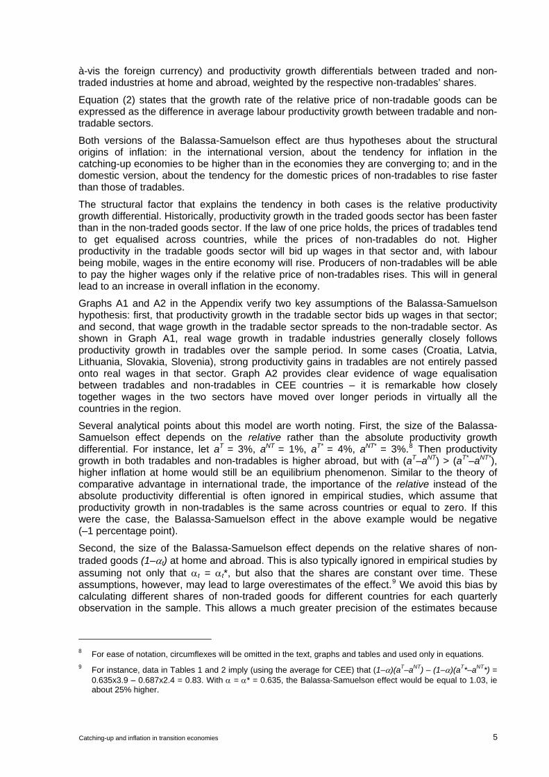
Table 1 summarises developments in productivity growth and inflation in 11 CEE countries and the euro area from an initial observation in the 1996–98 period to the first quarter of 2008. In line with the Balassa-Samuelson hypothesis, productivity growth was higher in tradable sectors, and relative prices increased faster in non-tradable sectors, in all 12 economies considered.14 However, no clear pattern between productivity differentials and relative price differentials seems to emerge at first sight: Slovakia, for instance, had the highest productivity differential and one of the lowest relative price differentials; while Bulgaria had the lowest productivity differential and one of the highest relative price differentials (Graph 1).

Yet when one looks at country averages, there seems to be strong support for the domestic Balassa-Samuelson hypothesis. More specifically, data in Table 1 suggest that the average productivity differential (aT – aNT) for 11 CEE countries (3.7 percentage points), corrected for the share of non-tradables (64%, shown in Table 2), was exactly equal to the sectoral price differential (pNT – pT) of 2.3 percentage points.

12 See, however, Égert et al (2006), pp. 12–13, for a version of equation (1) that allows the use of ALP in its own

right rather than as a proxy for total factor productivity. That version, however, can be used only in regressions with the real exchange rate as the dependent variable.

13 Using the Cobb-Douglas production function, (dY/Y) / (dL/L) = (dA/A) + (1–α) (dK/K) / (dL/L). 14 In the euro area, inflation of non-tradables was only marginally higher than that of tradables.


Table 1

Productivity growth and inflation in CEE1

Productivity growth Inflation Country (t0)

aT aNT aT – aNT2 P pNT – pT4P

3 pT pNT

Bulgaria (1998:Q2) 3.3 2.9 0.4 6.8 4.7 7.6 2.9

Croatia (1997:Q1) 5.2 2.3 2.9 3.4 2.8 5.9 3.1

Czech Rep. (1996:Q1) 6.3 2.8 3.5 3.6 1.6 4.0 2.4

Estonia (1997:Q1) 9.0 5.9 3.1 5.1 4.2 6.1 1.9

Hungary (1996:Q1) 6.0 2.1 3.9 8.4 8.0 8.1 0.1

Latvia (1998:Q2) 8.8 5.3 3.5 5.0 5.1 5.5 0.4

Lithuania (1996:Q1) 9.6 5.2 4.4 3.3 2.1 4.8 2.7

Poland (1997:Q1) 6.2 2.5 3.7 5.6 4.0 6.6 2.5

Romania (1997:Q1) 9.3 5.5 3.8 23.3 17.4 23.6 6.2

Slovakia (1996:Q1) 9.5 2.0 7.5 6.4 3.9 5.7 1.8

Slovenia (1996:Q3) 6.7 2.2 4.5 6.0 4.0 6.3 1.4

Average 7.3 3.5 3.7 7.0 5.3 7.7 2.3

Euro area (1997:Q1) 2.8 0.4 2.4 2.0 1.9 1.9 0.0 1 Four-quarter percentage changes, period averages (initial observation t0 shown in parentheses after the country name). T = tradables; NT = non-tradables. For the composition of tradable and non-tradable industries and price indices see the Appendix. 2 Difference between productivity growth in tradable and non-tradable sectors, in percentage points. 3 Overall CPI inflation. 4 Difference between inflation of non-tradable and tradable components of the CPI, in percentage points.

Graph 1

Domestic productivity growth and relative price differentials In percentage points, period average

7.5

4.5 4.43.9 3.8 3.7 3.5 3.5

3.1 2.92.4

0.4

1.81.4

2.7

0.1

6.2

2.5 2.4

0.4

1.9

3.1

0.0

2.9

0.0

2.0

4.0

6.0

8.0

SK SI LT HU RO PL CZ LV EE HR XM BG

d(aT – aNT)

d(pNT – pT)

Source: Authors’ calculations, based on the data described in the Appendix.


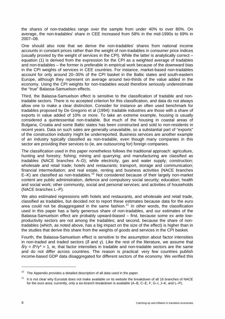
Table 2 summarises developments in productivity and inflation differentials of CEE countries vis-à-vis the euro area. All CEE countries recorded higher average annual inflation than the euro area over this period, with the differential ranging from around 1.3 percentage points in Croatia and Lithuania to more than 20 percentage points in Romania. All CEE countries (with the exception of Bulgaria) also achieved faster productivity growth in tradables vs. non-tradables than did the euro area. The sectoral productivity differential was on average equal to 1.6 percentage points, or 0.8 point when corrected for the share of non-tradables. This suggests that productivity differentials could explain only around 16% of the CEE countries’ average 5 percentage points inflation differential vis-à-vis the euro area. On this preliminary evidence, the international Balassa-Samuelson effect appears to be weaker than the domestic effect, which is in line with previous findings in the literature.

Table 2

Productivity and inflation differentials in CEE vis-à-vis the euro area1

Inflation differential

Change in nominal

exchange rate2

Sectoral productivity differential

Share of non-

tradables (%)

Balassa-Samuelson

effect3Country (t0)

p – p* e (aT – aNT)–(aT* – aNT*) (1 – α) (1–α)(aT–aNT)–

(1–α*)(aT*–aNT*)

Bulgaria (1998:Q2) 4.8 0.0 –2.0 62.7 –1.4

Croatia (1997:Q1) 1.4 0.6 0.5 56.5 –0.1

Czech R. (1996:Q1) 1.6 –2.3 1.1 62.2 0.5

Estonia (1997:Q1) 3.1 0.2 0.7 71.0 0.6

Hungary (1996:Q1) 6.4 2.5 1.5 59.6 0.7

Latvia (1998:Q2) 2.9 0.9 1.1 76.9 1.0

Lithuania (1996:Q1) 1.3 –3.2 4.4 66.4 1.3

Poland (1997:Q1) 3.6 1.4 1.3 67.5 0.8

Romania (1998:Q2) 21.3 14.4 1.4 53.6 0.2

Slovakia (1996:Q1) 4.4 –1.2 5.1 60.9 2.9

Slovenia (1996:Q3) 4.0 3.1 2.1 61.7 1.1

Average 5.0 1.5 1.6 63.5 0.8

Euro area (1997:Q1) … … 2.4 68.7 … 1 Four-quarter percentage changes, period averages (initial observation t0 shown in parentheses after the country name). 2 Negative sign denotes appreciation (fewer units of domestic currency per euro), positive depreciation. 3 Contribution of sectoral productivity differentials to the inflation differential vis-à-vis the euro area.

Changes in nominal exchange rates against the euro (a 1½ percentage point annual depreciation on average) explain around 30% of the CEE countries’ inflation differential vis-à-vis the euro area. It is quite surprising how stable, on average, nominal exchange rates have been over the past 10–12 years, including in the Czech Republic, Hungary and Poland, which had adopted inflation targeting and flexible exchange rate regimes. Because of this stability, even with a full pass-through of import prices to domestic inflation, the impact of exchange rate changes on domestic inflation – and hence on inflation differential vis-à-vis the euro area – seems to have been modest.


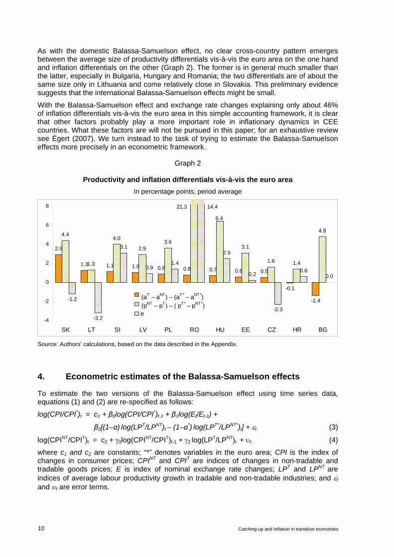
As with the domestic Balassa-Samuelson effect, no clear cross-country pattern emerges between the average size of productivity differentials vis-à-vis the euro area on the one hand and inflation differentials on the other (Graph 2). The former is in general much smaller than the latter, especially in Bulgaria, Hungary and Romania; the two differentials are of about the same size only in Lithuania and come relatively close in Slovakia. This preliminary evidence suggests that the international Balassa-Samuelson effects might be small.

With the Balassa-Samuelson effect and exchange rate changes explaining only about 46% of inflation differentials vis-à-vis the euro area in this simple accounting framework, it is clear that other factors probably play a more important role in inflationary dynamics in CEE countries. What these factors are will not be pursued in this paper; for an exhaustive review see Égert (2007). We turn instead to the task of trying to estimate the Balassa-Samuelson effects more precisely in an econometric framework.

Graph 2

Productivity and inflation differentials vis-à-vis the euro area In percentage points, period average

2.9

1.3 1.1 1.0 0.8 0.8 0.7 0.6 0.5

-0.1

-1.4

4.4

1.3

4.0

2.93.6

3.1

1.6 1.4

4.8

-1.2

-3.2

3.1

0.91.4

2.5

0.2

-2.3

0.60.0

6.4

-4

-2

0

2

4

6

8

SK LT SI LV PL RO HU EE CZ HR BG

e

(aT – aNT) – (aT* – aNT*) (pNT – pT) – ( pT* – pNT*)

21.3 14.4


4. Econometric estimates of the Balassa-Samuelson effects

To estimate the two versions of the Balassa-Samuelson effect using time series data, equations (1) and (2) are re-specified as follows:

log(CPI/CPI*)t = c1 + β0log(CPI/CPI*)t-1 + β1log(Et/Et-1) +

β2[(1–α) log(LPT/LPNT)t – (1–α*) log(LPT*/LPNT*)t] + εt (3)

log(CPINT/CPIT)t = c2 + γ0log(CPINT/CPIT)t-1 + γ2 log(LPT/LPNT)t

+ υt (4)

where c1 and c2 are constants; “*” denotes variables in the euro area; CPI is the index of changes in consumer prices; CPINT and CPIT are indices of changes in non-tradable and tradable goods prices; E is index of nominal exchange rate changes; LPT and LPNT

are indices of average labour productivity growth in tradable and non-tradable industries; and εt

and υt are error terms.


These two equations are estimated separately for each CEE country because we are interested in whether these effects might be a determining factor in the ability of each of these countries to meet the Maastricht inflation criterion. Admittedly, from an econometric perspective, pooling of the data for all countries or for groups of countries based on exchange rate regimes (eg, fixed vs floating regimes) or other criteria (eg, geographical region, size of the economy) and estimating panel regressions seems highly attractive. However, in the assessment of the Maastricht criteria, convergence reports are prepared for individual countries, not groups of countries. Moreover, as the results below will show, there is considerable heterogeneity among the countries in our sample, so pooling of the data might bias the estimates and make the interpretation of the results tenuous.

By construction, all regression variables are differenced – all productivity and price indices in equations (3) and (4) show seasonally adjusted, four-quarter percentage changes, and the exchange rate enters the regressions in the form (Et/Et-1). The stationarity of all time series was tested using the augmented Dickey-Fuller test. The results are not shown because of the large volume of test output.15 The vast majority of time series proved to be stationary in difference form with constant and/or with constant and trend, making it possible to use ordinary least squares to estimate the regression equations. This has significantly simplified the estimation procedure.

A lagged dependent variable is included on the right-hand side in both regressions. One reason is that the Breusch-Godfrey tests pointed to serial correlation of residuals in many regressions. Another is that we wanted to capture persistence in inflation differentials and, at the same time, allow the possibility of partial adjustment of inflation differentials to the changes in explanatory variables. The short-run Balassa-Samuelson elasticity is thus given by the coefficient β2, and long-run elasticity by β2/(1–β0).

Standard regression statistics are not reported. The fit of regressions is generally very good (adjusted R2 of 0.95 or higher), and standard test statistics are for the most part satisfactory. Many regressions of equation (4), and some of equation (3), initially had serially correlated residuals, but after applying standard transformations of lagged dependent variables, serial correlation was eliminated from most (though not all) regressions. As with the small number of non-stationary time series, it is highly unlikely that the presence of serial correlation in such a small number of cases could contaminate the estimates.

The estimates of the international Balassa-Samuelson effects are shown in Table 3. With few exceptions, all estimated parameters have the expected positive sign and are statistically significant at the 5% (or higher) test level. The estimates of the short-run Balassa-Samuelson coefficient β2 range from –0.10 (Croatia) to +0.19 (Hungary), and of the long-run coefficient from –1.3 (Croatia) to around 2.5 (Hungary, Lithuania and Romania). On average, the short-run Balassa-Samuelson coefficient is about 0.08 and the long-run coefficient is about 1.1.

15 There would be well over 400 test results to report: 12 different time series for 12 countries, each for 3 cases

(with constant, trend, constant and trend).


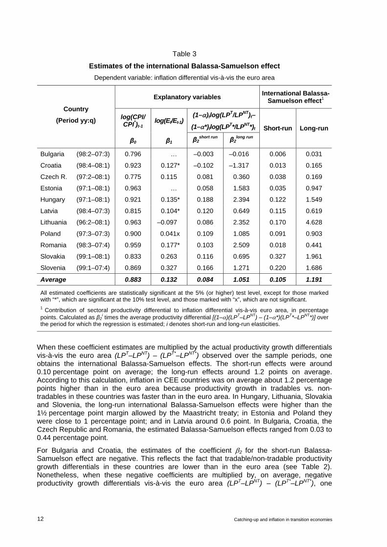
Table 3

Estimates of the international Balassa-Samuelson effectDependent variable: inflation differential vis-à-vis the euro area

International Balassa-Samuelson effect1Explanatory variables

log(CPI/CPI*)t-1

log(Et/Et-1)(1–α)tlog(LPT/LPNT)t–

(1–α*)tlog(LPT*/LPNT*)t

Country

(Period yy:q)

β0 β1 β2short run β2

long run

Short-run Long-run

Bulgaria (98:2–07:3) 0.796 … –0.003 –0.016 0.006 0.031

Croatia (98:4–08:1) 0.923 0.127* –0.102 –1.317 0.013 0.165

Czech R. (97:2–08:1) 0.775 0.115 0.081 0.360 0.038 0.169

Estonia (97:1–08:1) 0.963 … 0.058 1.583 0.035 0.947

Hungary (97:1–08:1) 0.921 0.135* 0.188 2.394 0.122 1.549

Latvia (98:4–07:3) 0.815 0.104* 0.120 0.649 0.115 0.619

Lithuania (96:2–08:1) 0.963 –0.097 0.086 2.352 0.170 4.628

Poland (97:3–07:3) 0.900 0.041x 0.109 1.085 0.091 0.903

Romania (98:3–07:4) 0.959 0.177* 0.103 2.509 0.018 0.441

Slovakia (99:1–08:1) 0.833 0.263 0.116 0.695 0.327 1.961

Slovenia (99:1–07:4) 0.869 0.327 0.166 1.271 0.220 1.686

Average 0.883 0.132 0.084 1.051 0.105 1.191

All estimated coefficients are statistically significant at the 5% (or higher) test level, except for those marked with “*”, which are significant at the 10% test level, and those marked with “x”, which are not significant. 1 Contribution of sectoral productivity differential to inflation differential vis-à-vis euro area, in percentage points. Calculated as β2

i times the average productivity differential [(1–α)(LPT–LPNT) – (1–α*)(LPT*–LPNT*)] over the period for which the regression is estimated; i denotes short-run and long-run elasticities.

When these coefficient estimates are multiplied by the actual productivity growth differentials vis-à-vis the euro area (LPT–LPNT) – (LPT*–LPNT*) observed over the sample periods, one obtains the international Balassa-Samuelson effects. The short-run effects were around 0.10 percentage point on average; the long-run effects around 1.2 points on average. According to this calculation, inflation in CEE countries was on average about 1.2 percentage points higher than in the euro area because productivity growth in tradables vs. non-tradables in these countries was faster than in the euro area. In Hungary, Lithuania, Slovakia and Slovenia, the long-run international Balassa-Samuelson effects were higher than the 1½ percentage point margin allowed by the Maastricht treaty; in Estonia and Poland they were close to 1 percentage point; and in Latvia around 0.6 point. In Bulgaria, Croatia, the Czech Republic and Romania, the estimated Balassa-Samuelson effects ranged from 0.03 to 0.44 percentage point.

For Bulgaria and Croatia, the estimates of the coefficient β2 for the short-run Balassa-Samuelson effect are negative. This reflects the fact that tradable/non-tradable productivity growth differentials in these countries are lower than in the euro area (see Table 2). Nonetheless, when these negative coefficients are multiplied by, on average, negative productivity growth differentials vis-à-vis the euro area (LPT–LPNT) – (LPT*–LPNT*), one


obtains positive international Balassa-Samuelson effects for both countries (Table 3, last two columns).

All CEE countries exhibit a fairly high persistence of inflation differentials vis-à-vis the euro area: estimates of the coefficient β0 range from around 0.80 in Bulgaria, the Czech Republic and Latvia to around 0.96 in Estonia, Lithuania and Romania, and all of them had the lowest standard errors.

Estimates of the pass-through of exchange rate changes to inflation differentials are less satisfactory. For Poland, no statistically significant estimate of the coefficient β1 could be obtained; for Lithuania the estimated coefficient was negative and highly significant; and for Hungary, Latvia and Romania it was significant at the 10% level only. Bulgaria and Estonia have kept fixed exchange rates against the euro over the sample period, so exchange rates were not included in their regressions. Latvia and Lithuania switched from their pegs to the SDR and the dollar, respectively, closer to 2004, when they joined the EU, so the results for these countries – in particular the negative exchange rate pass-through for Lithuania – are not entirely surprising. Interestingly, the highest pass-through of exchange rate changes to inflation differentials was observed in Slovenia and Slovakia, the only two countries in the sample that have fulfilled the Maastricht inflation criterion so far.

While these results on the whole suggest that the long-run Balassa-Samuelson effects in CEE might be fairly large, one should not jump to the conclusion that they support claims that the Maastricht inflation criterion needs to be reconsidered. The only countries for which the above regression estimates are very robust to small changes in specifications are the Czech Republic, Lithuania and Slovakia. For all other countries, small changes in initial or final observations, or in the lag structure of explanatory variables, often affected the size and statistical significance of the estimates.

Estimates of the domestic Balassa-Samuelson effects are shown in Table 4. All estimates of the coefficient γ2

s except one are statistically highly significant. However, the sign of the short-run Balassa-Samuelson coefficient for Hungary, Latvia and Lithuania is negative, although the size of the coefficient in each case is relatively small. In these three countries, faster productivity growth in tradable vs. non-tradable industries has been associated with a small decline in the relative price of non-tradables, contradicting the Balassa-Samuelson hypothesis. In all other countries, the coefficient on relative productivity growth has the expected positive sign; its size ranges from 0.05 (Poland) to 0.24 (Bulgaria).

Estimates of the coefficient γ0 on lagged relative price changes have the expected positive sign and are statistically highly significant. Their fairly large size indicates strong persistence of past relative price changes and also leads to high estimates of the long-run effects of differential productivity growth γ2

l.

The contribution of changes in relative productivity differentials (LPT–LPNT) to changes in relative price differentials (CPINT/CPIT) is obtained by multiplying the short-run and long-run coefficients γ2 with the respective average values of productivity differentials over the sample periods. These contributions amount on average to 0.22 percentage point in the short run and 1.94 points in the long run. Over the long run and on average, the domestic Balassa-Samuelson effects thus account for about 84% of the observed relative price differential of 2.3 percentage points.


Table 4

Estimates of the domestic Balassa-Samuelson effect Dependent variable: domestic relative price differential PNT/PT

Explanatory variables

log(CPINT/ CPIT)t-1

Log(LPT/LPNT)t

Contribution of (LPT/LPNT) to (CPINT/CPIT)

Domestic Balassa-Samuelson effect2Country

(Period yy:q)

γ0 γ2s γ2

l Short-run Long-run Short-run Long-run

Bulgaria (98:2–07:3) 0.873 0.244 1.924 0.103 0.811 0.065 0.509

Croatia (98:4–08:1) 0.794 0.121 0.584 0.320 1.552 0.181 0.877

Czech R. (97:2–08:1) 0.944 0.080 1.433 0.284 5.079 0.176 3.143

Estonia (97:1–08:1) 0.877 0.077* 0.628 0.315 2.561 0.223 1.814

Hungary (97:1–08:1) 0.878 –0.038 –0.308 –0.132 –1.079 –0.078 –0.640

Latvia (98:4–07:3) 0.897 –0.039 –0.377 –0.128 –1.248 –0.099 –0.963

Lithuania (96:2–08:1) 0.965 –0.036 –1.023 –0.156 –4.481 –0.103 –2.975

Poland (97:3–07:3) 0.950 0.045 0.890 0.165 3.290 0.111 2.221

Romania (98:3–07:4) 0.954 0.097 2.139 0.422 9.269 0.217 4.758

Slovakia (99:1–08:1) 0.740 0.109 0.418 0.880 3.383 0.531 2.044

Slovenia (99:1–07:4) 0.839 0.074 0.457 0.355 2.201 0.219 1.357

Average 0.883 0.067 0.615 0.221 1.940 0.131 1.104

All estimated coefficients are significant at the 1% test level, except the one for Estonia marked with “*”, which is significant at the 10% test level. 1 Contribution of the sectoral productivity differential (LPT–LP P

NT) to non-tradable/tradable goods inflation, in percentage points. Calculated as γ2

i times the average productivity differential observed over the sample period, where i denotes short-run and long-run elasticities. 2 Contribution of sectoral productivity differential (LPT–LPNT) to (CPINT/CPIT) adjusted for the share of non-tradables (1–α); in percentage points. This is a proxy for the contribution of (LPT–LPNT

P ) to overall inflation.

The contribution of relative productivity differentials to relative price differentials can be translated into the contribution to overall inflation as follows. Starting from the definition of consumer price inflation as a weighted average of tradable and non-tradable goods price inflation (equation 5):

NTt

Ttt ppp ˆ)1(ˆˆ αα −+= (5)

where α is the share of traded goods in the CPI basket, and using the expression for the relative price of non-tradables from equation (2) one obtains equation (6):

)ˆˆ)(1(ˆˆ NTt

Tt

Ttt aapp −−+= α (6)

Ie, the contribution of relative productivity differentials to overall inflation is proportionate to the share of non-tradables (1–α) multiplied by the contribution of relative productivity differentials to relative price differentials. This expression gives estimates of the domestic Balassa-Samuelson effect shown in the last two columns of Table 4. On average, the short-run effect amounts to 0.13 percentage point, and the long-run effect to 1.10 points. Faster growth of relative prices of non-tradables, resulting from faster growth of productivity in tradable relative to non-tradable industries, may thus have contributed on average around


1.10 percentage points to inflation in CEE countries over the long run. In other words, the domestic Balassa-Samuelson effect may on average explain only around 16% of overall domestic CPI inflation of 7% in CEE countries.

What is the evidence on the size of the Balassa-Samuelson effect over time?

In the simple accounting framework presented in Tables 1 and 2, the results are mixed. If we take the last quarter of 2001 as the mid-point of the sample, the international and domestic Balassa-Samuelson effects declined in the more recent sub-period (from 2002 to Q1:2008) in Bulgaria, Croatia, Hungary, Latvia and Slovakia; but increased in the Czech Republic, Estonia, Lithuania, Poland and Slovenia (Table 5).

Table 5

Balassa-Samuelson effect over time

Change in econometric estimates2Accounting framework1

International BSE Domestic BSE Country

t0–2001:Q4 2002:Q1– 2008:Q1 t0–2001:Q4 2002:Q1–

2008:Q1

Inter-national

BSE Domestic

BSE

Bulgaria 0.7 –2.8 0.7 –2.8 no Δ ↓

Croatia 0.8 –0.5 4.7 1.7 ↓ ↓

Czech Republic –0.3 1.1 2.6 4.2 no Δ ↑

Estonia –1.4 1.9 4.2 4.7 no Δ ↓

Hungary 0.7 0.6 4.3 3.6 no Δ ↓

Lithuania –0.5 2.7 2.1 6.2 ↓ ↑

Latvia 2.3 0.5 4.2 2.6 no Δ no Δ

Poland –0.5 2.0 2.0 5.1 no Δ ↓

Romania –1.0 1.1 2.3 5.0 ↓ ↓

Slovakia 3.4 2.3 8.2 7.7 ↑ no Δ

Slovenia 1.1 1.6 3.8 5.0 no Δ no Δ 1 Based on the historical data summarised in Tables 1 and 2. 2 Based on the estimates of regression equations (3) and (4) for two sub-periods of the main mid-1990s–2008:Q1 period (determined for each country by Chow breakpoint tests). The entries indicate no change (no Δ), increase (↑) or decrease (↓) in the estimated Balassa-Samuelson coefficient between the earlier and later periods.

The results of econometric estimates are also mixed. For the international effect, the Chow breakpoint test indicated the presence of a structural breakpoint in the series for differential productivity growth (LPT–LPNT)–(LPT*–LPNT*) for only four countries: Croatia (at 2004:Q1), Lithuania (2000:Q1), Romania (2001:Q2) and Slovakia (2002:Q1). Evidence on changes in the size of the short-run Balassa-Samuelson coefficient β2

s in the respective sub-periods was mixed. The size of the coefficient declined in the second sub-period (ie, from the breakpoint through 2008:Q1) in Croatia, Lithuania and Romania, but increased substantially in Slovakia. These estimates are unreliable, however, because of the short length of the time series and – in the case of Croatia, Romania and Slovakia – the long time lags (7–10 quarters) with which differential productivity growth affects inflation differentials vis-à-vis the euro area.


For the domestic Balassa-Samuelson effect, the Chow breakpoint test indicated the presence of a structural breakpoint in the (LPT/LPNT) series for all the countries except Latvia, Slovenia and Slovakia. The breakpoints were at 2002:Q1 for Bulgaria, Croatia and Romania; 2003:Q1 for the Czech Republic, Estonia, Hungary and Poland; and 2001:Q1 for Lithuania. The size of the short-run coefficient γ2

s declined in the second, more-recent sub-period in Bulgaria, Croatia, Estonia, Hungary, Poland and Romania, reflecting the slowing of productivity growth in tradables vs. non-tradables in recent years compared with the second half of the 1990s. The coefficient γ2

s increased in the more recent sub-period only in the Czech Republic and Lithuania. Because of the short length of the time series, these sub-period estimates of the domestic Balassa-Samuelson effects are less reliable than the estimates shown in Table 4, though on the whole they are somewhat better than those for the international effect by sub-periods.

5. Concluding remarks

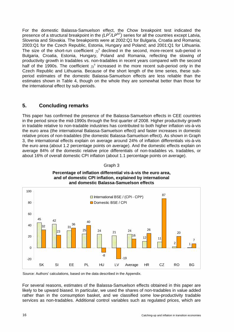
This paper has confirmed the presence of the Balassa-Samuelson effects in CEE countries in the period since the mid-1990s through the first quarter of 2008. Higher productivity growth in tradable relative to non-tradable industries has contributed to both higher inflation vis-à-vis the euro area (the international Balassa-Samuelson effect) and faster increases in domestic relative prices of non-tradables (the domestic Balassa-Samuelson effect). As shown in Graph 3, the international effects explain on average around 24% of inflation differentials vis-à-vis the euro area (about 1.2 percentage points on average). And the domestic effects explain on average 84% of the domestic relative price differentials of non-tradables vs. tradables, or about 16% of overall domestic CPI inflation (about 1.1 percentage points on average).

Graph 3

Percentage of inflation differential vis-à-vis the euro area, and of domestic CPI inflation, explained by international

and domestic Balassa-Samuelson effects

45 42

3125 24 21 24

12 112 1

3223

3640

-8

16

26

87

20

7

-19-20

0

20

40

60

80

100

SK SI EE PL HU LV Average HR CZ RO BG

International BSE / (CPI - CPI*) Domestic BSE / CPI


For several reasons, estimates of the Balassa-Samuelson effects obtained in this paper are likely to be upward biased. In particular, we used the shares of non-tradables in value added rather than in the consumption basket, and we classified some low-productivity tradable services as non-tradables. Additional control variables such as regulated prices, which are


important in non-tradable sectors, might have also reduced the estimated size of the Balassa-Samuelson effects. However, by extending our sample to a larger number of countries and a much longer period – including the important sector of agriculture in tradables – and especially by using country- and time-specific shares of non-tradables, we have obtained more precise and representative estimates of the Balassa-Samuelson effects than have other available studies.

Real convergence since the early 2000s seems to have reduced the domestic Balassa-Samuelson effects in several countries and the international effects in somewhat fewer countries. But for several countries, the size of both effects may have increased.

The experience of Slovenia and Slovakia, both of which have relatively strong Balassa-Samuelson effects vis-à-vis the euro area (estimated at 2.0 and 1.7 percentage points, respectively), shows that it is possible to fulfil the Maastricht inflation criterion even if these effects might be higher than the 1½ percentage point margin allowed by the Maastricht treaty. At the same time, it cannot be ruled out that a strong Balassa-Samuelson effect could complicate the policy tradeoffs for some EMU candidate countries. Arguably, Lithuania’s strong Balassa-Samuelson effect, estimated at 4.6 percentage points, may have been one of the factors behind the country’s unsuccessful bid to join the euro area in 2007. This suggests that the Balassa-Samuelson effects are likely to remain on the policy and research agenda for a while, given that the pace of catching-up is likely to remain uneven across countries seeking to join EMU.

Against this background, one should perhaps caution against attempts to start using estimates of the Balassa-Samuelson effects in policy assessment. Obtaining precise and reliable estimates of these effects is much more difficult than, for instance, obtaining estimates of potential GDP. In particular, measurement errors and room for discretion in transforming the data and applying even the simplest estimating procedures are not negligible. Issues of equal treatment would inevitably arise if one sought to standardise these estimating procedures in practice. Therefore, one would be hard pressed to recommend, in good confidence, an operationalisation of the concept of the Balassa-Samuelson effect for the assessment of the Maastricht inflation criterion.


Appendix

Data description Traded and non-traded sectors

Traded goods and services: agriculture, forestry and hunting; fishing; mining and quarrying; manufacturing.

Non-traded goods and services: electricity, gas and water supply; construction; wholesale and retail trade, repair of motor vehicles, personal and household goods; transport, storage and communication; financial intermediation; real estate, renting and business activities.

Not included are public administration, defence and compulsory social security; education; health and social work; other community, social and personal services; and activities of household.

Description of variables

• Quarterly indices of value added growth (in constant prices) from the production-side estimates of GDP. Sectors are aggregated into traded and non-traded using industries’ shares in total value added in a given quarter.

• CPI rates of inflation with subcomponents (quarterly averages of monthly rates). The breakdown into traded and non-traded goods and services followed the production-side classification as closely as possible. However, the complete matching of sectors with price indices was not always possible. The subcomponents are aggregated into traded and non-traded goods inflation using their weights in the CPI basket.

• Nominal exchange rates of domestic currency against the euro (quarterly averages of daily rates).

• Employment (total number of workers, quarterly averages of monthly figures) in traded and non-traded goods industries following the above classification. Employment in traded and non-traded sectors obtained from industries’ shares in total employment (quarterly averages).

Data transformations

• All variables entering regressions are first expressed in terms of chain indices showing four-quarter percentage changes, with 1999:Q4 = 100.

• For some initial observations in the mid-1990s (sectoral breakdown of value added and employment), quarterly data were linearly interpolated from annual data.

• All indices are then seasonally adjusted using the X-12 procedure.

• Finally, natural logarithms of seasonally adjusted indices are taken.

• These time series are tested for stationarity using the augmented Dickey-Fuller unit root test.

Data sources Eurostat; national central banks and statistical offices; European Central Bank; BIS Data Bank; BIS staff estimates.


Appendix Graph A1

Productivity and wages in tradable industries 2000:Q4 = 100; not seasonally adjusted

20

40

60

80

100

120

140

1996 1998 2000 2002 2004 2006 2008

Productivity tradable BGReal wages tradable BG

60

80

100

120

140

160

180

1996 1998 2000 2002 2004 2006 2008

Productivity tradable CZReal wages tradable CZ

80

90

100

110

120

130

140

150

1996 1998 2000 2002 2004 2006 2008

Productivity tradable HRReal wages tradable HR

60

80

100

120

140

160

180

200

220

1996 1998 2000 2002 2004 2006 2008

Productivity tradable EEReal wages tradable EE

60

80

100

120

140

160

180

1996 1998 2000 2002 2004 2006 2008

Productivity tradable HUReal wages tradable HU

60

80

100

120

140

160

180

200

1996 1998 2000 2002 2004 2006 2008

Productivity tradable LVReal wages tradable LV


Appendix Graph A1 (cont)

Productivity and wages in tradable industries 2000:Q4 = 100; not seasonally adjusted

40

80

120

160

200

240

280

1996 1998 2000 2002 2004 2006 2008

Productivity tradable LTReal wages tradable LT

60

80

100

120

140

160

180

1996 1998 2000 2002 2004 2006 2008

Productivity tradable PLReal wages tradable PL

50

75

100

125

150

175

200

225

250

1996 1998 2000 2002 2004 2006 2008

Productivity tradable ROReal wages tradable RO

60

80

100

120

140

160

180

200

220

1996 1998 2000 2002 2004 2006 2008

Productivity tradable SKReal wages tradable SK

60

80

100

120

140

160

180

1996 1998 2000 2002 2004 2006 2008

Productivity tradable SIReal wages tradable SI


Appendix Graph A2

Wages in tradable and non-tradable industries 2000:Q4 = 100; not seasonally adjusted

0

40

80

120

160

200

240

1996 1998 2000 2002 2004 2006 2008

Wage tradable BGWage non tradable BG

80

90

100

110

120

130

140

1996 1998 2000 2002 2004 2006 2008

Wage tradable HRWage non tradable HR

40

60

80

100

120

140

160

180

1996 1998 2000 2002 2004 2006 2008

Wage tradable CZWage non tradable CZ

40

80

120

160

200

240

1996 1998 2000 2002 2004 2006 2008

Wage tradable EEWage non tradable EE

0

40

80

120

160

200

1996 1998 2000 2002 2004 2006 2008

Wage tradable HUWage non tradable HU

40

80

120

160

200

240

280

1996 1998 2000 2002 2004 2006 2008

Wage tradable LVWage non tradable LV


Appendix Graph A2 (cont)

Wages in tradable and non-tradable industries 2000:Q4 = 100; not seasonally adjusted

40

60

80

100

120

140

160

180

200

1996 1998 2000 2002 2004 2006 2008

Wage tradable LTWage non tradable LT

20

40

60

80

100

120

140

160

180

1996 1998 2000 2002 2004 2006 2008

Wage tradable PLWage non tradable PL

0

100

200

300

400

500

1996 1998 2000 2002 2004 2006 2008

Wage tradable ROWage non tradable RO

40

60

80

100

120

140

160

180

200

1996 1998 2000 2002 2004 2006 2008

Wage tradable SKWage non tradable SK

40

60

80

100

120

140

160

180

1996 1998 2000 2002 2004 2006 2008

Wage tradable SIWage non tradable SI


References

Alberola-Ila E and T Tyrväinen (1998): “Is there scope for inflation differentials in EMU? An empirical evaluation of the Balassa-Samuelson model in EMU”, Banco de España Working Paper no 9823.

Begg, D, B Eichengreen, L Halpern, J von Hagen and C Wyplosz (2003): “Sustainable Regimes of Capital Movements in Accession Countries”, CEPR Policy Paper no 10.

Buiter, W and A Siebert (2006): “The inflation criterion for Eurozone membership: what to do when you fail to meet it?” paper prepared for the Annual Meeting of the Turkish Economic Association, Ankara, 11 September.

Buiter W and C Grafe (2002): “Anchor, Float or Abandon Ship: Exchange Rate Regimes for the Accession Countries”, European Investment Bank Papers, 7(2), 51–71.

Burgess R, S Fabrizio and Y Xiao (2003): “Competitiveness in the Baltics in the run-up to EU accession”, IMF Country Report no 03/114. www.imf.org.

Chukalev, G (2002): “The Balassa-Samuelson effect in the Bulgarian economy”, Working Paper of the Bulgarian Agency for Economic Analysis and Forecasting.

Cincibuch, M and J Podpiera (2006): “Beyond Balassa-Samuelson: real appreciation in tradables and transition countries”, Economics of Transition, vol 14, no 3, 547-573.

Cipriani, M (2001): The Balassa-Samuelson effect in transition economies, unpublished manuscript, IMF, Washington, September.

Coricelli, F and B Jazbec (2001): “Real exchange rate dynamics in transition economies”, Structural Change and Economic Dynamics, vol 15, 83–100.

Darvas, Z and G Szapáry (2008): “Euro area enlargement and euro adoption strategies”, European Commission, Economic Papers No. 304, February.

De Gregorio, J, A Giovannini and H Wolf (1994): “International evidence on tradables and nontradables inflation”, European Economic Review, 38, 1225–44.

Deroose, S and J Baras (2005): “The Maastricht criteria on price and exchange rate stability and ERM II”, in S Schadler (ed), Euro adoption in central and eastern Europe: opportunities and challenges, IMF, Washington, 128–41.

Égert, B (2007): “Real convergence, price convergence and inflation differentials in Europe”, CESifo Working Paper No 2127, October.

——— (2005a): “Balassa-Samuelson meets south-eastern Europe, the CIS and Turkey: a close encounter of the third kind?” European Journal of Comparative Economics, Vol 2 no 2, 221–234.

——— (2005b): “The Balassa-Samuelson hypothesis in Estonia: oil shale, tradable goods, regulated prices and other culprits”, World Economy, vol 28, no 2, 259–286.

——— (2003): “Assessing equilibrium exchange rates in CEE acceding countries: can we have DEER with BEER without FEER? A critical survey of the literature”, Focus on Transition, no 2, 38–106.

——— (2002a): “Estimating the Balassa-Samuelson effect on inflation and the real exchange rate during the transition”, Economic Systems, 26, 1–16.

——— (2002b): “Investigating the Balassa-Samuelson hypothesis in transition: do we understand what we see? A panel study”, Economics of Transition, vol 10, 273–309.

Égert, B and J Podpiera (2008): “Structural inflation and real exchange rate appreciation in Visegrad-4 countries: Balassa-Samuelson or something else?” CEPR Policy Insight no 20, April. www.cepr.org.


http://www.imf.org/

http://www.cepr.org/

Égert, B, I Drine, K Lommatzsch and C Rault (2003): “The Balassa-Samuelson effect in central and eastern Europe: myth or reality”, Journal of Comparative Economics, Vol 31, 552–572.

Égert, B, L Halpern and R MacDonald (2006): “Equilibrium exchange rates in transition economies: taking stock of the issues”, Journal of Economic Surveys, Vol 20, no 2, 257–324.

Flek, V, L Marková and J Podpiera (2002): “Sectoral productivity and real exchange rate appreciation: much ado about nothing?” Czech National Bank Working Paper, no 4.

Funda, J, G Lukinić and I Ljubaj (2007): “Assessment of the Balassa-Samuelson effect in Croatia”, Financial Theory and Practice, vol 31, no 4, 321–351. www.ijf.hr.

Golinelli, R and R Orsi (2002): “Modelling inflation in EU accession countries: the case of the Czech Republic, Hungary and Poland”, in W Charmeza and K Strzala (eds) East European transition and EU enlargement: a quantitative approach, Berlin: Springer, 267–290.

Halpern, L and C Wyplosz (2001): “Economic transformation and real exchange rates in the 2000s: the Balassa-Samuelson connection”, Economic Survey of Europe, no 1, Geneva, United Nations Economic Commission for Europe.

Kovács, M (ed) (2002): “On the estimated size of the Balassa-Samuelson effect in five central and eastern European countries”, MNB Working Paper, no 5/2002. www.mnb.hu.

Kovács, M and A Simon (1998): “Components of the real exchange rate in Hungary”, National Bank of Hungary Working Paper, no 1998/3.

Lojschova, A (2003): “Estimating the impact of the Balassa-Samuelson effect in transition economies”, Institute for Advanced Studies (Vienna), Working Paper no 140.

MacDonald, R and C Wojcik (2004): “Catching-up: the role of demand, supply and regulated price effects on the real exchange rates of four accession countries”, Economics of Transition, vol 12, 153–179.

Mihaljek, D (2008): “The financial stability implications of increased capital inflows for emerging market economies”, forthcoming in BIS Papers.

——— (2006): “Are the Maastricht criteria appropriate for central and eastern Europe?” in S Motamen-Samadian (ed), Economic Transition in Central and Eastern European Countries, Cheltenham: Palgrave.

Mihaljek, D and M Klau (2007): “The Balassa-Samuelson effect and the Maastricht criteria: revisiting the debate”, in N Batini (ed), Monetary Policy in Emerging Markets and Other Developing Countries, New York: Nova Science Publishers.

——— (2004): “The Balassa-Samuelson effect in central Europe: a disaggregated analysis”, Comparative Economic Studies, vol 46, March, 63–94.

Nenovsky N and K Dimitrova (2002): “Dual inflation under the currency board: the challenges of Bulgarian EU accession”, William Davidson Institute Working Paper no 487.

Padoa-Schioppa, T (2003): “Trajectories towards the euro and the role of ERM II”, in Gertrude Tumpel-Gugerell and Peter Mooslechner (eds), Structural Challenges for Europe, Edward Elgar, 405–412.

Rother, P (2000): “The impact of productivity differentials on inflation and the real exchange rate: an estimation of the Balassa-Samuelson effect in Slovenia”, in Republic of Slovenia: Selected issues, IMF Staff Country Report no 00/56.

Szapáry, G (2000): “Maastricht and the choice of the exchange rate regime in the transition countries during the run-up to EMU”, National Bank of Hungary Working Paper no 2000/7.

Wagner M and J Hlouskova (2004): “What is really the story with the Balassa-Samuelson effect in the CEECs”, University of Bern, Economics Department Discussion Paper no 04/16.


http://www.ijf.hr/

http://www.mbb.hu/

bis working papers · samuelson effect for these countries is therefore of particular interest....

Documents