BIOLOGICAL - ENVIRONMENTAL CLASSIFICATION (BEC) SYSTEM AND

SUPPORTING FLOW – BIOLOGY RELATIONSHIPS IN NORTH CAROLINA –

PROJECT UPDATE

Conducted by: RTI and USGS

Funded by: Environmental Defense Fund, North Carolina Division of Water Resources, North Carolina Wildlife Resources Commission

BACKGROUND

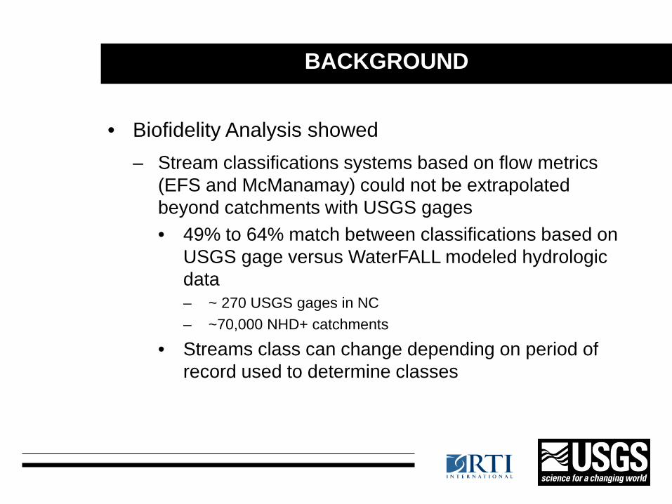
• Biofidelity Analysis showed – Stream classifications systems based on flow metrics

(EFS and McManamay) could not be extrapolated beyond catchments with USGS gages • 49% to 64% match between classifications based on

USGS gage versus WaterFALL modeled hydrologic data – ~ 270 USGS gages in NC – ~70,000 NHD+ catchments

• Streams class can change depending on period of record used to determine classes

BACKGROUND

• Conclusion – Need a classification system that

• Is not based on sensitive threshold values • Is consistent and reproducible using USGS stream

gage and modeled data • Is easy to understand and implement • Can be applied throughout state • Captures the distribution of aquatic biota in North

Carolina

3

OBJECTIVES OF BEC PROJECT

1. Develop a classification system based on geographical assemblages of aquatic biota (fish and benthos) and associated environmental (physiographic and hydrologic) attributes – Biological-Environmental Classification (BEC) system

2. Determine flow–biology response relationships for each BEC class

3. Link significant flow metrics (and associated flow–biology relationships) to each BEC class to support ecological flow determinations

Step 1 – Determine BEC classes based on aquatic biota assemblages and environmental characteristics

Step 2 – Determine flow-biology relationships for each BEC class

Step 3 – Link significant flow metrics to each BEC class to support determination of ecological flows

CLASSIFICATION BASED ON ENVIRONMENTAL ATTRIBUTES

CLUSTERING OF ENVIRONMENTAL FACTORS

1. NHD drainage area

2. Cumulative drainage area

3. NHD slope

4. Slope

5. Elevation

6. Minimum elevation

7. Relief (max−min elev)

8. % flat land (<1% slope)

9. % flat low land

10. % flat uplands

11. Precipitation

12. Evapotranspiration

13. Precip-Evapotransp.

14. Temperature

15. Sinuosity

16. Aquifer permeability

17. % sand in soils

CORRELATIONS (SPEARMAN) AMONG ENVIRONMENTAL VARIABLES

CumDA Precip

NHD Slope

Sinuosity Elev % SAND DA Temp

AQUIFER PERM SLOPE PET PMPE MINELE RELIEF

% FLAT TOT

% FLAT LOW

% FLAT UP

CumDA Precip -0.129 NHDSlope -0.478 0.192 Sinu -0.091 0.072 0.083 Elev -0.159 0.284 0.497 -0.024 SAND -0.034 0.336 -0.101 0.027 -0.337 DA -0.006 0.069 -0.029 0.869 -0.111 0.066 Temp 0.107 -0.185 -0.457 0.064 -0.894 0.327 0.156 AQIFER PERM 0.038 0.108 -0.344 0.039 -0.756 0.701 0.125 0.717 SLOPE -0.081 0.304 0.505 -0.049 0.930 -0.292 -0.144 -0.855 -0.719 PET 0.074 -0.199 -0.439 0.064 -0.897 0.334 0.159 0.964 0.739 -0.865 PMPE -0.089 0.791 0.302 0.019 0.614 0.108 -0.021 -0.571 -0.215 0.614 -0.607 MINELE -0.078 0.268 0.460 -0.045 0.983 -0.350 -0.133 -0.889 -0.770 0.930 -0.904 0.615 RELIEF -0.080 0.308 0.499 -0.053 0.899 -0.245 -0.144 -0.828 -0.668 0.953 -0.839 0.584 0.882 % FLAT TOT 0.081 -0.330 -0.489 0.048 -0.923 0.305 0.134 0.854 0.712 -0.978 0.868 -0.636 -0.921 -0.937 %F LAT LOW 0.096 -0.445 -0.432 0.025 -0.765 0.142 0.091 0.698 0.504 -0.806 0.705 -0.663 -0.758 -0.750 0.821 % FLAT UP 0.059 -0.350 -0.392 0.033 -0.777 0.168 0.102 0.760 0.537 -0.808 0.787 -0.639 -0.785 -0.814 0.819 0.478

Environmental variables selected for cluster analysis: Cumulative drainage area Sinuosity Precipitation % Sand in soil Elevation NHD slope

|r|≥ 0.7

ENVIR VAR: FULL VS. REDUCED MATRIX

Environmental variables: Full vs. Reduced MatrixRELATE analysis

-0.1 0 0.1 0.2 0.3 0.4 0.5 0.6 0.7 0.8Rho

0

211

Freq

uenc

y

Distributions of correlation base on permutations

Correlation between full and reduced similarity metrics

RELATE Analysis

Rho

Freq

uenc

y

CLUSTER ANALYSIS: ENVIRONMENTAL VARIABLES

• Partitioning around medoids (PAM) • Standardized data (mean = 0, sd = 1) • Euclidean distance • Examined 2-60 clusters • Average silhouette used to determine “best”

clustering • Box plots of variables in “best” clustering

0 5 10 15 20 25 30

0.00

0.05

0.10

0.15

0.20

0.25

0.30

0.35

pam() clustering assessment

k (# clusters)

aver

age

silh

ouet

te w

idth

best7

“BEST” CLUSTERING OF ENVIR. VARIABLES

Number of Clusters

Aver

age

Silh

ouet

te W

idth

0.71-1.00: Strong structure 0.51-0.70: Reasonable structure 0.26-0.50: Weak structure <0.25: No structure

1 2 3 4 5 6 7

050

010

0015

00Elevation

Cluster

% E

lev

ELEVATION

Cluster

Elev

atio

n (m

)

1 2 3 4 5 6 7

050

100

150

NHD Drainage Area

Cluster

Dra

inag

e ar

ea

NHD DRAINAGE AREA

Cluster

Elev

atio

n (m

)

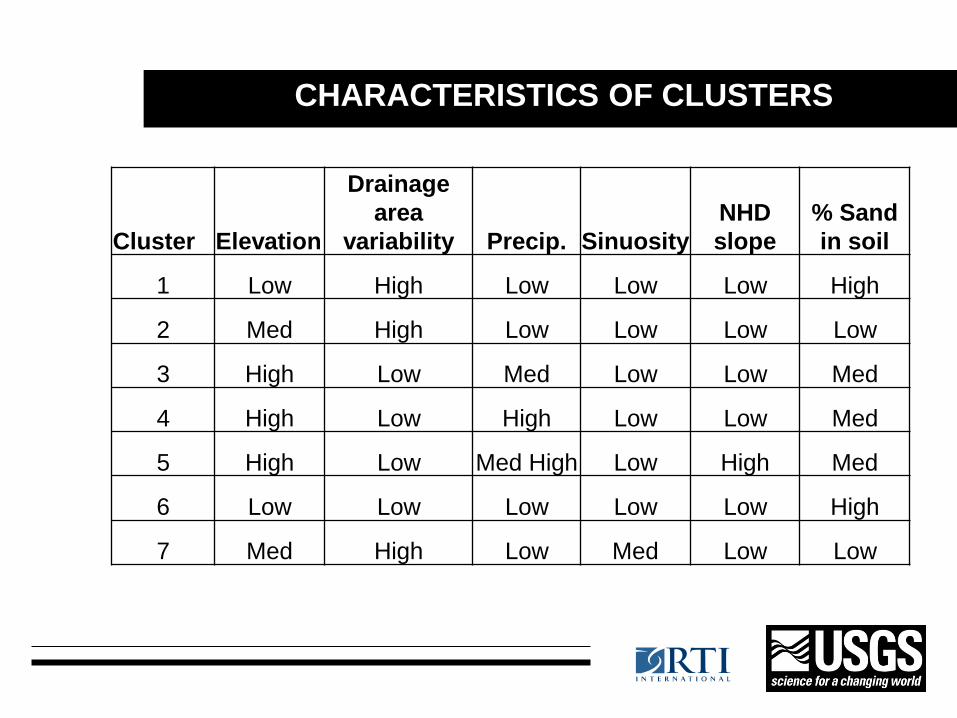
CHARACTERISTICS OF CLUSTERS

Cluster Elevation

Drainage area

variability Precip. Sinuosity NHD slope

% Sand in soil

1 Low High Low Low Low High

2 Med High Low Low Low Low

3 High Low Med Low Low Med

4 High Low High Low Low Med

5 High Low Med High Low High Med

6 Low Low Low Low Low High

7 Med High Low Med Low Low

ENVIRONMENTAL CLUSTERS

1 2 3 4 5 6 7

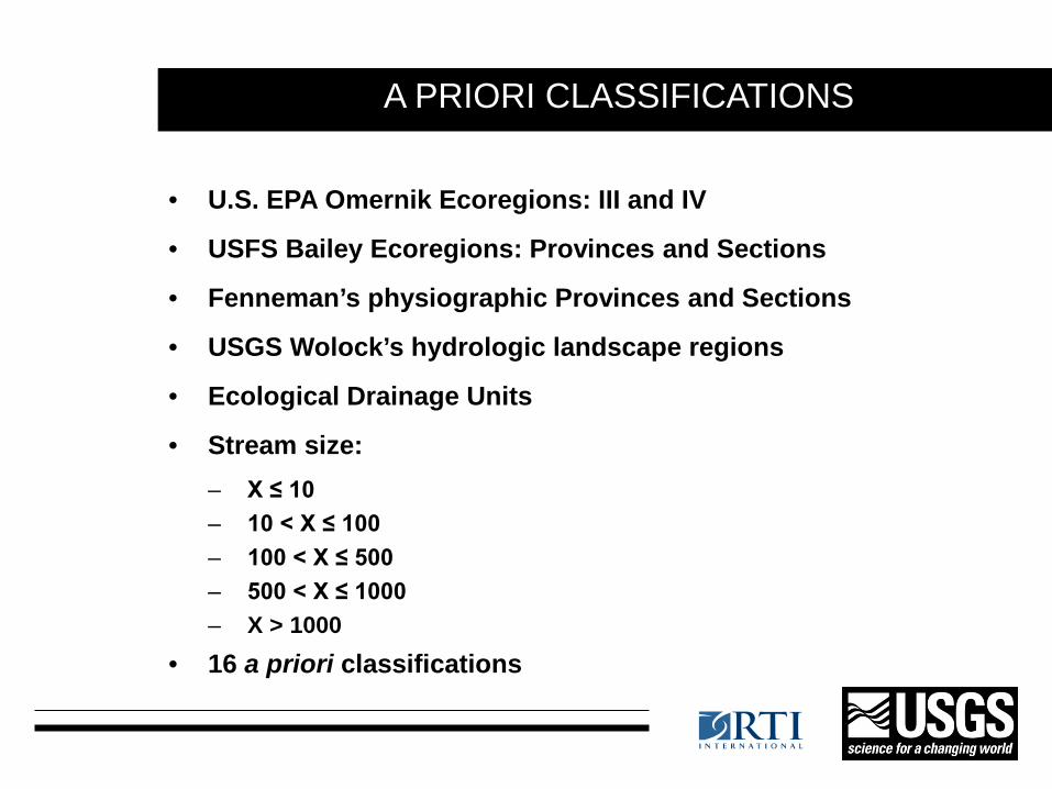
A PRIORI CLASSIFICATIONS

• U.S. EPA Omernik Ecoregions: III and IV

• USFS Bailey Ecoregions: Provinces and Sections

• Fenneman’s physiographic Provinces and Sections

• USGS Wolock’s hydrologic landscape regions

• Ecological Drainage Units

• Stream size: – X ≤ 10 – 10 < X ≤ 100 – 100 < X ≤ 500 – 500 < X ≤ 1000 – X > 1000

• 16 a priori classifications

0.30

0.40

0.50

0.60

0.70

0.80

ER II

I

ER II

I DA

ER IV

ER IV

DA

FEN

PR

OV

FEN

PR

OV

DA

FEN

SEC

FEN

SEC

DA

BA

ILEY

PR

OV

BA

ILEY

PR

OV

DA

BA

ILEY

SEC

BA

ILEY

SEC

DA

WO

LOC

K

WO

LOC

K D

A

EDU

EDU

DA

PAM

Clu

s7

r-st

atis

tic

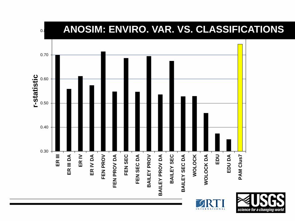
ANOSIM: environmental variables vs. a priori and "best" PAM cluster

ANOSIM: ENVIRO. VAR. VS. CLASSIFICATIONS

CLASSIFICATION BASED ON INVERTEBRATE BIOTA

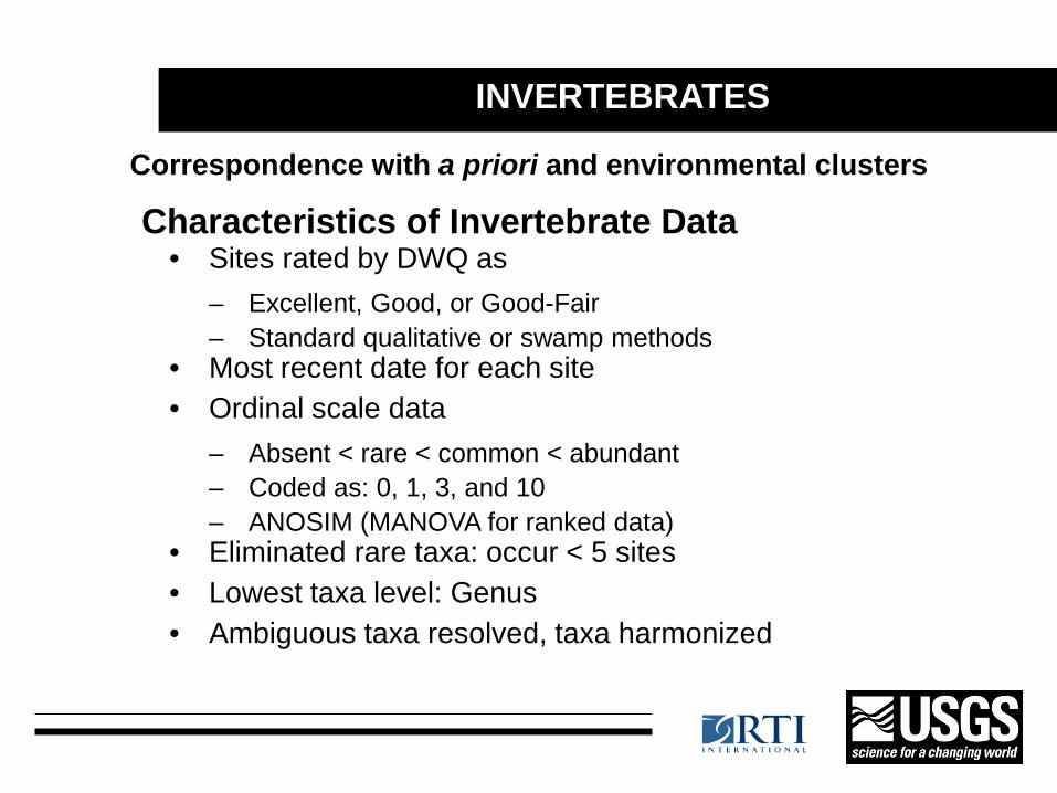
INVERTEBRATES

• Sites rated by DWQ as – Excellent, Good, or Good-Fair – Standard qualitative or swamp methods

• Most recent date for each site • Ordinal scale data

– Absent < rare < common < abundant – Coded as: 0, 1, 3, and 10 – ANOSIM (MANOVA for ranked data)

• Eliminated rare taxa: occur < 5 sites • Lowest taxa level: Genus • Ambiguous taxa resolved, taxa harmonized

Correspondence with a priori and environmental clusters

Characteristics of Invertebrate Data

0.25

0.27

0.29

0.31

0.33

0.35

0.37

0.39

2 4 6 8 10 12 14 16 18 20 22 24 26 28 30 32 34 36 38 40 42 44 46 48 50 52 54 56 58 60

r-st

atis

tic

Number of Clusters

ANOSIM: Envir. clusters (PAM) applied to invertebrate community

ANOSIM: PAM CLUSTERS VS. INVERTEBRATES

0.25

0.27

0.29

0.31

0.33

0.35

0.37

0.39

0.41

0.43

0.45

ER II

I

ER II

I DA

ER IV

ER IV

DA

FEN

PR

OV

FEN

PR

OV

DA

FEN

SEC

FEN

SEC

DA

BA

ILEY

PR

OV

BA

ILEY

PR

OV

DA

BA

ILEY

SEC

BA

ILEY

SEC

DA

WO

LOC

K

WO

LOC

K D

A

EDU

EDU

DA

Pam

Clu

s7

r-st

atis

tic

s vs. a priori classifications ANOSIM: A PRIORI CLASSIFICATIONS AND INVERTS

INVERTEBRATE: CLUSTERING

• Evaluated multiple clustering methods – K-means: uses Euclidean distance – PAM: Bray-Curtis, very low silhouette values – Hierarchical clustering (Bray-Curtis):

• Agglomerative: many small clusters • Divisive hierarchical clustering: “best” clustering?

• Examined 2-60 clusters

• ANOSIM to assess correspondence between clusters

and invert data (similarity matrix)

INVERTS: PAM CLUSTERING

0.00

0.02

0.04

0.06

0.08

0.10

0.12

0 10 20 30 40 50 60

Avg.

Silh

ouet

te W

idth

Number of Clusters

0.71-1.00: Strong structure 0.51-0.70: Reasonable structure 0.26-0.50: Weak structure <0.25: No structure

ANOSIM: ENV CLUSTERED BY INVERTEBRATES

0.00

0.05

0.10

0.15

0.20

0.25

0.30

0.35

0.40

0 10 20 30 40 50 60

r-st

atis

tic

Number of Invertebrate Clusters

Inverts: Divisive hierarchical clustering Envir: Euclidean similarity matrix

LINKING INVERTS AND ENV: CART ANALYSIS ELEV < 242.9

MINELE < 58.8 NHDSlope < 0.008255

ANOSIM: A PRIORI & NMDS CART CLUSTERS

0.2

0.25

0.3

0.35

0.4

0.45

0.5

Eco

Reg

III

Eco

Reg

III D

A

Eco

Reg

IV

Eco

Reg

IV D

A

FEN

PRO

V

FEN

PRO

V D

A

FEN

SEC

FEN

SEC

DA

WO

LOCK

WO

LOCK

DA

ECO

DRA

IN U

NIT

S

ECO

DRA

IN U

NIT

S DA

BAIL

EY P

ROV

BAIL

EY P

ROV

DA

BAIL

EY S

EC

BAIL

EY S

EC D

A

CART

2

CART

3a

CART

3b

CART

4

CART

8

CART

9

ANO

SIM

r-st

atis

tic

NUMBER CLASSES

0

10

20

30

40

50

60

70

80

Eco

Reg

III

Eco

Reg

III D

A

Eco

Reg

IV

Eco

Reg

IV D

A

FEN

PRO

V

FEN

PRO

V D

A

FEN

SEC

FEN

SEC

DA

WO

LOCK

WO

LOCK

DA

ECO

DRA

IN U

NIT

S

ECO

DRA

IN U

NIT

S DA

BAIL

EY P

ROV

BAIL

EY P

ROV

DA

BAIL

EY S

EC

BAIL

EY S

EC D

A

CART

2

CART

3a

CART

3b

CART

4

CART

8

CART

9

No.

cla

sses

NON-SIGNIFICANT PAIRWISE CLASSES

0.0

10.0

20.0

30.0

40.0

50.0

60.0

Eco

Reg

III

Eco

Reg

III D

A

Eco

Reg

IV

Eco

Reg

IV D

A

FEN

PRO

V

FEN

PRO

V D

A

FEN

SEC

FEN

SEC

DA

WO

LOCK

WO

LOCK

DA

ECO

DRA

IN U

NIT

S

ECO

DRA

IN U

NIT

S DA

BAIL

EY P

ROV

BAIL

EY P

ROV

DA

BAIL

EY S

EC

BAIL

EY S

EC D

A

CART

2

CART

3a

CART

3b

CART

4

CART

8

CART

9

% n

on-s

igni

fican

t (p,

0.05

)

NEXT STEPS FOR INVERT ANALYSES

• Derive invertebrate metrics (aggregations of species attributes) with emphasis on those sensitive to flow (e.g., filter-feeders, collector-gatherers)

• Directly related invertebrate metrics to environmental variables (CART) to develop integrated classifications

• Relate invertebrate metrics to flow variables: – Flow surplus/deficit and IHA metrics – CART analysis (identify important flow variables) – Analyses (e.g., quantile regression)

• Within classes • State-wide

• Repeat analyses at species level

CLASSIFICATION BASED ON FISH

STREAM FISH COMMUNITY DATA

Data Description and Formatting Most recent sample at 858 unique XY

coordinate locations Count data at species level Data was log transformed Species observed at <5 sites were removed Sample locations with no fish were removed Bray-Curtis method used to calculate

dissimilarity matrix

ANALYTICAL APPROACH

Environmental Classifications – Associate sample locations and community data with

eco-region level, drainage class, and USGS-derived environmental clusters

– Test explanatory power of each classification (PERMANOVA)

Biological Classification – Use community data to create biology-based groups

with PAM and hierarchical agglomerative techniques – Test significance and explanatory power (Silhouette

width, multi-scale bootstrap re-sampling, PERMANOVA)

ENVIRONMENTAL CLASSIFICATIONS

BIOLOGICAL CLUSTERS: PAM

BIOLOGICAL CLUSTERS: HIERARCHICAL

Bootstrap Sampling alpha=0.5 n=62 clusters

BIOLOGICAL CLUSTERS: HIERARCHICAL

k=8

Cluster Freq Elev Slope Drain 1 86 2555 3.93 23 2 166 107 0.14 72 3 82 1235 0.93 45 4 205 522 0.24 77 5 82 386 0.24 118 6 51 1101 2.75 61 7 77 812 0.43 68 8 108 2094 0.91 77

Cluster Freq Elev Slope Drain 1 86 2593 1.85 14 2 166 58 0.10 47 3 82 1127 0.49 40 4 205 541 0.16 58 5 82 335 0.17 64 6 51 468 0.27 58 7 77 830 0.27 55 8 108 2072 0.65 51

Mean Values

Median Values

GEOGRAPHIC DISTRIBUTION; HIER K=8

CLUSTER/CLASS SIZE COMPARISON

NEXT STEPS FOR FISH

Cluster Analysis – Incorporate select environmental variables into biological

clustering process – Assess cluster p-values in terms of centers and

multivariate spread

NEXT STEPS FOR FISH

Classification – Classify ‘best’ cluster results in terms of environmental

variables; assess predictive power using 80/20 training/test regime

1 2 3 4 5 6 7 8 1 24 0 1 0 0 3 0 8 2 0 47 0 12 7 5 0 0 3 0 0 16 4 2 0 9 0 4 0 1 3 34 1 4 8 0 5 0 0 0 4 13 2 0 0 6 1 0 0 0 0 2 0 0 7 0 0 1 9 2 0 3 0 8 1 0 6 0 0 0 0 18

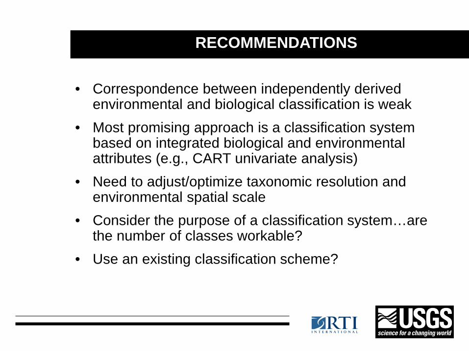
RECOMMENDATIONS

• Correspondence between independently derived environmental and biological classification is weak

• Most promising approach is a classification system based on integrated biological and environmental attributes (e.g., CART univariate analysis)

• Need to adjust/optimize taxonomic resolution and environmental spatial scale

• Consider the purpose of a classification system…are the number of classes workable?

• Use an existing classification scheme?