bidirectional seiching in a rectangular, open channel

22ème

Congrès Français de Mécanique Lyon, 24 au 28 Août 2015

Bidirectional seiching in a rectangular, open

channel, lateral cavity

E. MIGNOTa, M. POZET

a, N. RIVIERE

a, S. CHESNE

b

a. Université de Lyon, LMFA, INSA, Bat. Jacquard, 20 av. A. Einstein, 69621 Villeurbanne,

France – [email protected]

b. Université de Lyon, CNRS INSA-Lyon, LaMCoS UMR5259, F-69621, Villeurbanne,

France

Résumé :

Le travail présenté ici s’intéresse aux oscillations de surface libre de cavités latérales, c’est à dire des

cavités horizontales à surface libre connectées sur un de leur côté à un écoulement permanent. Ce

phénomène d’oscillation, appelé Seiching, est étudié expérimentalement, tout d’abord pour une cavité

carrée, puis pour une cavité rectangulaire. Les oscillations de surface libre sont mesurées et, pour la

cavité carrée, deux ondes stationnaires coexistantes apparaissent et sont chacune reconstruites en

utilisant des méthodes d’analyse de signal. De plus, il apparaît que les fréquences d’oscillation

correspondantes sont en bon accord avec les pics de fréquence du spectre de vitesse mesuré dans la

couche de mélange. Finalement, pour la cavité rectangulaire l’onde stationnaire d’axe

perpendiculaire à l’écoulement principal disparaît et une nouvelle onde d’axe longitudinal apparait

dans la cavité.

Abstract :

The present work is dedicated to the free-surface oscillation of lateral cavities, i.e. horizontal cavities

with free surface connected along one of their sides to a steady main flow. This oscillation

phenomenon, named seiching, is studied experimentally, first for a square cavity and then for a

rectangular one. Water surface oscillations are recorded and, for the square cavity, two standing

waves of perpendicular axes appear to co-exist and are reconstructed individually using usual signal

processing tools. Moreover, the corresponding oscillation frequencies appear to be well correlated

with the peak frequencies of the velocity spectrum in the mixing layer. Finally, for the rectangular

cavity, the standing wave of axis perpendicular to the mainstream axis disappears and an additional

standing wave of streamwise axis appears.

Mots clefs : Seiching; free-surface oscillation; lateral cavity; mixing layer;

peak frequency

22ème


1 Introduction and theoretical background Present work is dedicated to open-channel lateral cavities, i.e. horizontal cavities with free surface

connected along one of their sides to a main free-surface flow. Such cavities are encountered in

various natural (oxbows, cut-off meanders) or artificial (harbors connected to a river) open-channel

hydrodynamic situations.

1.1 Flow pattern in the cavity The flow in the mainstream is permanent while the cavity is initially at rest. Nevertheless, the transfer

of momentum from the mainstream towards the cavity creates a flow in the cavity: one or several

recirculation cells occurs in the cavity depending on the width to length aspect ratio of the cavity (see

Riviere et al., 2010). For a square cavity where the width (W) and length (L) of the cavity (see Fig.2)

are equal, several authors reveal that a single horizontal cell occupies most of the available space in

the cavity, with a typical velocity about 1/8 of the main stream cavity (see Cai et al., 2014). This

strong velocity gradient between the main stream and the cavity leads to a mixing layer aligned along

the interface between the two regions, that is along the segment joining the upstream and downstream

corners of the cavity (see Fig.2).

1.2 Coherent structures in the mixing layer As expressed by several authors in simple mixing layers (Loucks and Wallace, 2012) or in mixing

layers at the interface of an open-channel lateral cavity (Sanjou et al., 2012; Sanjou and Nezu, 2013),

coherent turbulent structures (named eddies in the present text) are generated near the upstream corner

of the mixing layer and are advected along the mixing layer towards the downstream corner. These

eddies cause an alternation of rapid and slow streamwise velocity components. Thus, as when

impacting on the downstream corner the kinetic energy of the flow is transferred to potential energy

and causes a water depth rise at the stagnatuion point,the streamwise velocity fluctuation at the

downstream corner creates a fluctuating local water depth. As a consequence, small waves propagate

in all directions, including within the cavity.

1.3 Frequency of the passing eddies The frequency at which the eddies are created and impact the downstream corner and generate small

waves is a function of the geometry of the mixing layer and the velocity gradient across the mixing

layer, which is itself a function of the velocity of the recirculation cell in the cavity, itself a function of

the momentum transfer from the main stream towards the cavity which depends on the characteristics

of the mixing layer. The system is then strongly interdependent, and to our knowledge, no method

exist to predict the frequency of the passing eddies .

1.4 Seiching phenomenon If the natural frequency of the cavity is in agreement with the eddies passing frequency, the oscillation

of the free-surface amplifies and the so-called seiching takes place, with free-surface oscillations that

can reach 1.5 meter on the field (Refmar, 2014). The natural frequency of a cavity is computed as

follows. For a cavity with a simplified rectangular shape, Wüest and Farmer (2003) or Sorensen and

Thompson (2006) explain that Merian formula relates the width of the cavity W (or its length L, see

Fig.2), the water depth in the cavity h and the possible seiche frequency fnat (equal to the natural

frequency of the cavity) as:

22ème


W

ghnfnat

2 (1)

That is the wave length nat equals:

n

Wnat

2 (2)

with n being an integer.

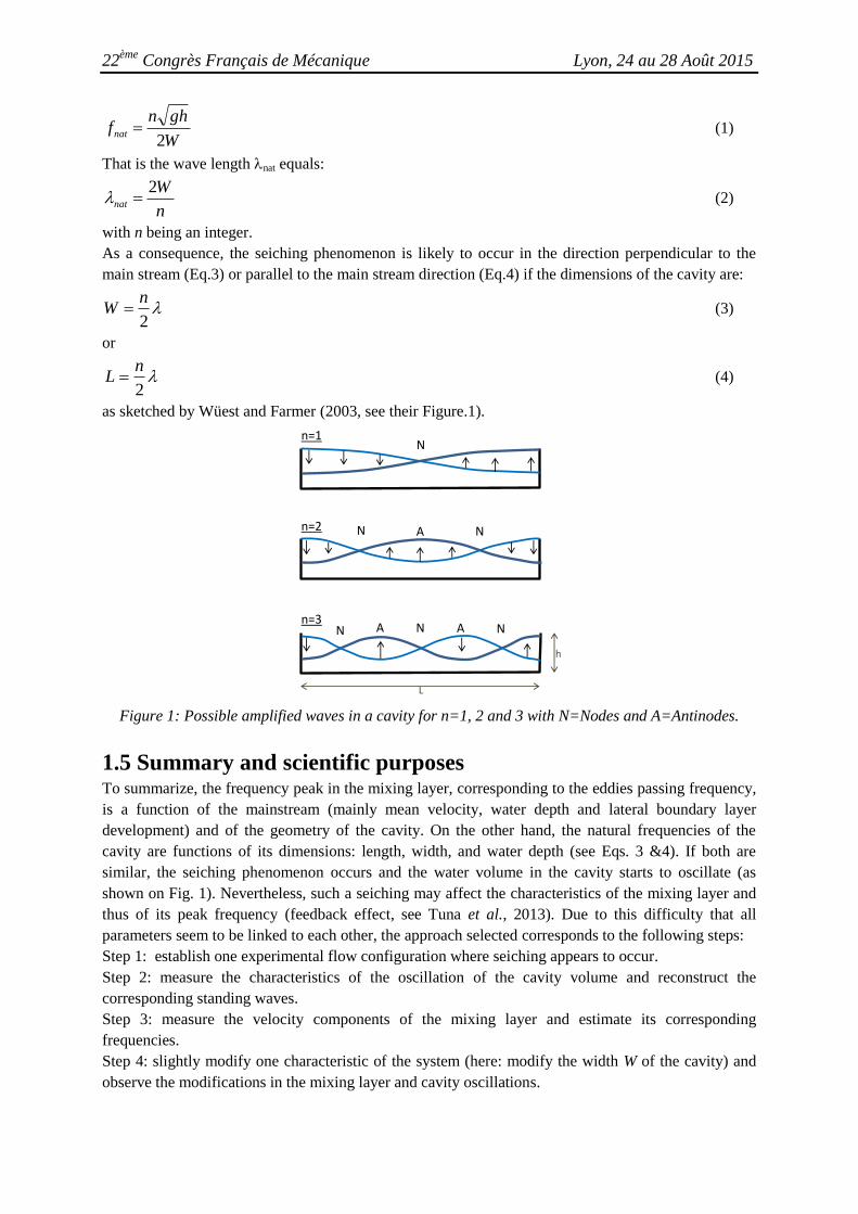
As a consequence, the seiching phenomenon is likely to occur in the direction perpendicular to the

main stream (Eq.3) or parallel to the main stream direction (Eq.4) if the dimensions of the cavity are:

2

nW (3)

or

2

nL (4)

as sketched by Wüest and Farmer (2003, see their Figure.1).

n=1N

n=2 N NA

n=3N NA AN

L

h

Figure 1: Possible amplified waves in a cavity for n=1, 2 and 3 with N=Nodes and A=Antinodes.

1.5 Summary and scientific purposes To summarize, the frequency peak in the mixing layer, corresponding to the eddies passing frequency,

is a function of the mainstream (mainly mean velocity, water depth and lateral boundary layer

development) and of the geometry of the cavity. On the other hand, the natural frequencies of the

cavity are functions of its dimensions: length, width, and water depth (see Eqs. 3 &4). If both are

similar, the seiching phenomenon occurs and the water volume in the cavity starts to oscillate (as

shown on Fig. 1). Nevertheless, such a seiching may affect the characteristics of the mixing layer and

thus of its peak frequency (feedback effect, see Tuna et al., 2013). Due to this difficulty that all

parameters seem to be linked to each other, the approach selected corresponds to the following steps:

Step 1: establish one experimental flow configuration where seiching appears to occur.

Step 2: measure the characteristics of the oscillation of the cavity volume and reconstruct the

corresponding standing waves.

Step 3: measure the velocity components of the mixing layer and estimate its corresponding

frequencies.

Step 4: slightly modify one characteristic of the system (here: modify the width W of the cavity) and

observe the modifications in the mixing layer and cavity oscillations.

22ème


2. Experimental set-up

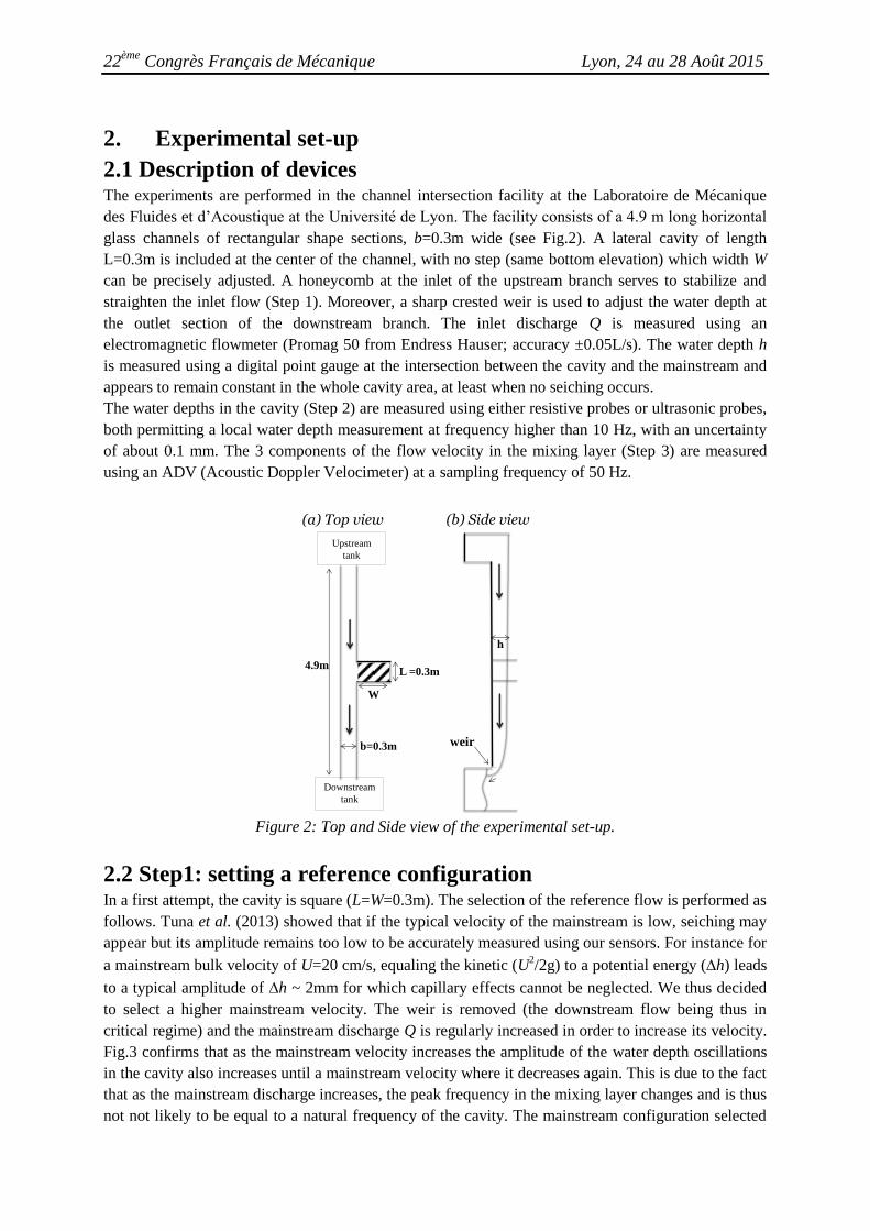
2.1 Description of devices The experiments are performed in the channel intersection facility at the Laboratoire de Mécanique

des Fluides et d’Acoustique at the Université de Lyon. The facility consists of a 4.9 m long horizontal

glass channels of rectangular shape sections, b=0.3m wide (see Fig.2). A lateral cavity of length

L=0.3m is included at the center of the channel, with no step (same bottom elevation) which width W

can be precisely adjusted. A honeycomb at the inlet of the upstream branch serves to stabilize and

straighten the inlet flow (Step 1). Moreover, a sharp crested weir is used to adjust the water depth at

the outlet section of the downstream branch. The inlet discharge Q is measured using an

electromagnetic flowmeter (Promag 50 from Endress Hauser; accuracy ±0.05L/s). The water depth h

is measured using a digital point gauge at the intersection between the cavity and the mainstream and

appears to remain constant in the whole cavity area, at least when no seiching occurs.

The water depths in the cavity (Step 2) are measured using either resistive probes or ultrasonic probes,

both permitting a local water depth measurement at frequency higher than 10 Hz, with an uncertainty

of about 0.1 mm. The 3 components of the flow velocity in the mixing layer (Step 3) are measured

using an ADV (Acoustic Doppler Velocimeter) at a sampling frequency of 50 Hz.

(a) Top view (b) Side view

weir

h

Upstream

tank

Downstream

tank

4.9m

b=0.3m

W

L =0.3m

Figure 2: Top and Side view of the experimental set-up.

2.2 Step1: setting a reference configuration In a first attempt, the cavity is square (L=W=0.3m). The selection of the reference flow is performed as

follows. Tuna et al. (2013) showed that if the typical velocity of the mainstream is low, seiching may

appear but its amplitude remains too low to be accurately measured using our sensors. For instance for

a mainstream bulk velocity of U=20 cm/s, equaling the kinetic (U2/2g) to a potential energy (h) leads

to a typical amplitude of h ~ 2mm for which capillary effects cannot be neglected. We thus decided

to select a higher mainstream velocity. The weir is removed (the downstream flow being thus in

critical regime) and the mainstream discharge Q is regularly increased in order to increase its velocity.

Fig.3 confirms that as the mainstream velocity increases the amplitude of the water depth oscillations

in the cavity also increases until a mainstream velocity where it decreases again. This is due to the fact

that as the mainstream discharge increases, the peak frequency in the mixing layer changes and is thus

not not likely to be equal to a natural frequency of the cavity. The mainstream configuration selected

22ème


as reference configuration is finally the one within the red circle. The reference configuration is thus

L=W=0.3m, U=47cm/s, h=6cm, and the gravity waves celerity smghc /77.0 .

1

2

L

W 1

1,5

2

2,5

3

3,5

4

4,5

5

5,5

6

0,35 0,4 0,45 0,5

Am

plit

ud

e o

f o

scill

atio

ns

(mm

)

Mainstream velocity (m/s)

Capteur 1

Capteur 2

Sensor 1

Sensor 2

Figure 3: Amplitude of the square cavity oscillation measured at two locations 1 and 2 for an

increasing mainstream velocity.

3. Results for the reference configuration

3.1 Step 2: measurement of the water depth oscillation in the

cavity Once the reference configuration is set, a seiching phenomenon is observed and the aim of the present

section is to identify all characteristics of the oscillation pattern. To do so, a preliminary work consists

of locating a water depth sensor measuring the water depth oscillation during about a minute near the

upstream-extremity corner of the cavity as sketched on Fig.4a. The corresponding power spectral

density, plotted on Fig.4b reveals two peak frequencies f1=0.5859Hz and f2=1.27Hz, which should

then correspond to two standing waves. Application of Eq.1 reveals that the natural frequencies of the

cavity for the reference configuration are:

- for a length L=0.3m, n=1 (half a wavelength, see Fig.1) leads to fnat-1=1.279Hz quite similar to f2,

corresponding to wave 1 in Fig.4c

- for a length b+W=2W=0.6m, n=2 (one wavelength) leads to fnat-2=1.279Hz, quite similar to f2

corresponding to wave 2 in Fig.4c.

- for a length b+W=2W=0.6m, n=1 (half a wavelength) leads to fnat-3=0.639Hz quite similar to f1

corresponding to wave 3 in Fig.4c.

The measured frequency f2 could then correspond to the waves 1 or 2 sketched on Fig.4c. Indeed

waves 1 and 2 present the same wavelength due to particular dimension of the set up (2L=b+w).

Frequency f1 seems to correspond to wave 3.

L

W

Po

wer

sp

ectr

al d

ensi

ty

Frequency (Hz) b=0,3m

L=0,3m

W=0,3m

12

3

(a) (b) (c)

Figure 4: Location of the sensor (a) and corresponding water depth power spectrum (b); possible

sketch of the possible standing wave following these results

22ème


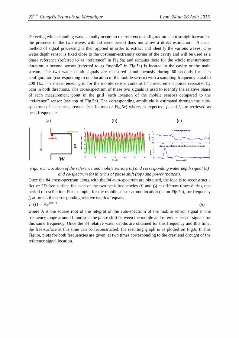
Detecting which standing wave actually occurs in the reference configuration is not straightforward as

the presence of the two waves with different period does not allow a direct estimation. A usual

method of signal processing is then applied in order to extract and identify the various waves. One

water depth sensor is fixed close to the upstream-extremity corner of the cavity and will be used as a

phase reference (referred to as “reference” in Fig.5a) and remains there for the whole measurement

duration; a second sensor (referred to as “mobile” in Fig.5a) is located in the cavity or the main

stream. The two water depth signals are measured simultaneously during 60 seconds for each

configuration (corresponding to one location of the mobile sensor) with a sampling frequency equal to

200 Hz. The measurement grid for the mobile sensor contains 84 measurement points separated by

5cm in both directions. The cross-spectrum of these two signals is used to identify the relative phase

of each measurement point in the grid (each location of the mobile sensor) compared to the

“reference” sensor (see top of Fig.5c). The corresponding amplitude is estimated through the auto-

spectrum of each measurement (see bottom of Fig.5c) where, as expected, f1 and f2 are retrieved as

peak frequencies.

L

W

Cross-spectrumreference

mobile

Time (s)

Wat

er d

epth

(m

m)

Frequency (Hz)

Ph

ase

( )

Po

wer

(a) (b) (c)

Auto-spectrum of mobile sensor signal

Figure 5: Location of the reference and mobile sensors (a) and corresponding water depth signal (b)

and co-spectrum (c) in terms of phase shift (top) and power (bottom).

Once the 84 cross-spectrum along with the 84 auto-spectrum are obtained, the idea is to reconstruct a

fictive 2D free-surface for each of the two peak frequencies (f1 and f2) at different times during one

period of oscillation. For example, for the mobile sensor at one location (as on Fig.5a), for frequency

f1 at time t, the corresponding relative depth h’ equals: tiAeth )(' (5)

where A is the square root of the integral of the auto-spectrum of the mobile sensor signal in the

frequency range around f1 and is the phase shift between the mobile and reference sensor signals for

this same frequency. Once the 84 relative water depths are obtained for this frequency and this time,

the free-surface at this time can be reconstructed; the resulting graph is as plotted on Fig.6. In this

Figure, plots for both frequencies are given, at two times corresponding to the crest and drought of the

reference signal location.

22ème


a

b

c

d

3

2

1

0

-1

-2

-3

dh (mm)

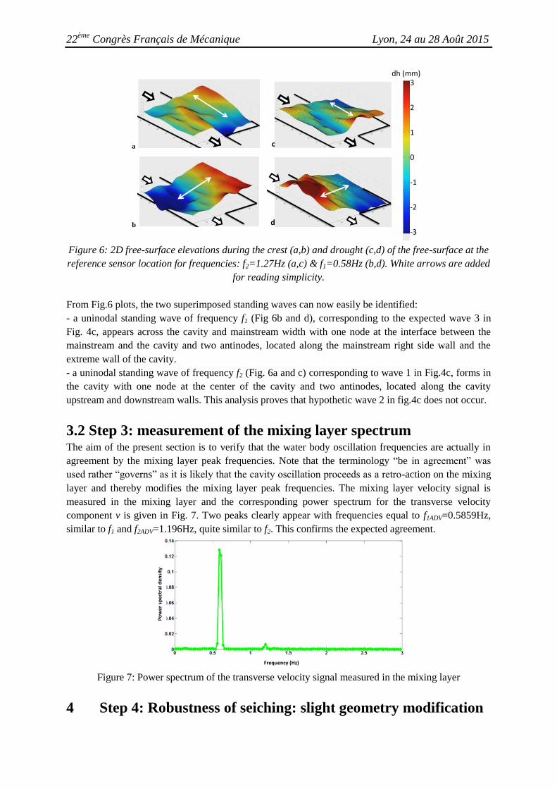
Figure 6: 2D free-surface elevations during the crest (a,b) and drought (c,d) of the free-surface at the

reference sensor location for frequencies: f2=1.27Hz (a,c) & f1=0.58Hz (b,d). White arrows are added

for reading simplicity.

From Fig.6 plots, the two superimposed standing waves can now easily be identified:

- a uninodal standing wave of frequency f1 (Fig 6b and d), corresponding to the expected wave 3 in

Fig. 4c, appears across the cavity and mainstream width with one node at the interface between the

mainstream and the cavity and two antinodes, located along the mainstream right side wall and the

extreme wall of the cavity.

- a uninodal standing wave of frequency f2 (Fig. 6a and c) corresponding to wave 1 in Fig.4c, forms in

the cavity with one node at the center of the cavity and two antinodes, located along the cavity

upstream and downstream walls. This analysis proves that hypothetic wave 2 in fig.4c does not occur.

3.2 Step 3: measurement of the mixing layer spectrum The aim of the present section is to verify that the water body oscillation frequencies are actually in

agreement by the mixing layer peak frequencies. Note that the terminology “be in agreement” was

used rather “governs” as it is likely that the cavity oscillation proceeds as a retro-action on the mixing

layer and thereby modifies the mixing layer peak frequencies. The mixing layer velocity signal is

measured in the mixing layer and the corresponding power spectrum for the transverse velocity

component v is given in Fig. 7. Two peaks clearly appear with frequencies equal to f1ADV=0.5859Hz,

similar to f1 and f2ADV=1.196Hz, quite similar to f2. This confirms the expected agreement.

Po

wer

sp

ectr

al d

ensi

ty

Frequency (Hz)

Figure 7: Power spectrum of the transverse velocity signal measured in the mixing layer

4 Step 4: Robustness of seiching: slight geometry modification

22ème


The aim of the present section (step 4) is to measure the influence of a slight modification of the cavity

width W on the cavity oscillation: the cavity width is increased to W’=0.35m, all other parameters

remaining fixed. The consequences in terms of mixing-layer oscillations compared to the square cavity

configuration are that:

- the frequency peak near f1ADV (~0.6Hz) almost completely disappeared (see Fig. 8a) so as the

corresponding transverse standing wave 3 in the cavity (not shown here).

- the velocity frequency peak f2ADV remains high (see Fig. 8a), so as the corresponding

transverse standing wave 1 in the cavity (not shown here).

- a new peak at frequency f3ADV=2.59Hz appears, which equals to the natural frequency

fnat=2.56Hz of the cavity corresponding to the length L=0.3m and n=2. This new standing wave is thus

binodal and occurs along the same direction as the uninodal one of frequency f2 (see Fig. 8b, c).

1.27 Hz

2.59Hz0.59Hz

(a) (b) (c)

Po

we

r sp

ect

ral d

en

sity

Frequency (Hz) Figure 8: Increased width cavity: transverse velocity power spectrum measured in the mixing layer

(a) and reconstruction of the 2D free-surface for the new frequency f3 during the crest (b) and drought

(c) at the reference sensor location.

Conclusions The seiching phenomenon, i.e. sustained oscillations of the free surface, was studied experimentally in

a lateral, open-channel cavity with adjustable dimensions. Water surface oscillations were recorded

and correlated with velocity measurements in the mixing layer and their corresponding frequency

spectra.

- To the authors’ knowledge, cavities investigated in the literature have dimensions (w+b) and L that

are not multiples of each other. Hence, natural frequencies are different in the streamwise and

crosswise directions and seiches form in only one direction. The present study, with a cavity such as

(w+b)=2L in steps 1, 2 and 3 proves that seiching can develop simultaneously in streamwise and

crosswise directions.

- The use of usual signal processing tools allows isolating the different waves constituting the water

body oscillation, which frequencies correspond to the natural frequencies of the cavity

- The robustness of the phenomenon was tested. A modification so small as (w+b)=2.17L makes the

crosswise wave disappear. It is replaced by a second streamwise wave, binodal, that adds to the first,

uninodal one.

Future work must be devoted to the interaction phenomena observed. First one is the interaction of

waves of different frequencies, where the largest amplitude can pass from one wave to another.

Second is the feedback phenomenon from the seiche to the mixing layer, where two frequency peaks

are clearly visible.

References Cai W., Brosset M., Mignot E., & Riviere N., 2014. Measurement of mass exchange between a main

flow and an adjacent lateral cavity. In International Conference on Fluvial Hydraulics (River Flow

2014), Lausanne, Switzerland.

22ème


Loucks R.B., & Wallace J.M., 2012. Velocity and velocity gradient based properties of a turbulent

plane mixing-layer. J. of Fluid Mech. 699, 280–319.

Refmar (Réseaux de référence des observations marégraphiques). Seiche. 2014. Available at:

http://refmar.shom.fr/fr/applications_maregraphiques/etudes-meteo-oceaniques/seiche

Riviere N., Garcia M., Mignot E., & Travin G., 2010. Characteristics of the recirculation cell pattern

in a lateral cavity. In International Conference on Fluvial Hydraulics (River Flow 2010),

Braunschweig, Germany, p. 673 .

Sanjou M., Akimoto T., & Okamoto T., 2012. Three-dimensional turbulence structure of rectangular

side-cavity zone in open channel streams. Int. J. River Basin Management 10 (4), 293–305.

Sanjou M., & Nezu I., 2013 Hydrodynamic characteristics and related mass-transfer properties in

open-channel flows with rectangular embayment zone. Environ Fluid Mech. 13 (6), 527–555.

Sorensen R., & Thompson E., 2006. Harbor hydrodynamics. Chapter 7.

Tuna B.A., Tinar E., & Rockwell, D., 2013. Shallow flow past a cavity: globally coupled oscillations

as a function of depth. Exp. in Fluids 54, 1586.

Wüest A., & Farmer D.M., 2003. Seiches. McGraw-Hill encyclopedia of science & technology.

bidirectional seiching in a rectangular, open channel

Documents