1

Best Practices for SSD Performance Measurement

Overview The performance of solid state drives (SSDs) can vary over time. SSDs are sensitive to their write-history, to how full their capacity is and to system variations, which means that SSDs have unique requirements to accurately measure performance in a repeatable and meaningful way. In this technical marketing brief we’ll highlight best practices for measuring Enterprise SSD performance, with an emphasis on the following points:

• Main goals of performance measurement (accuracy, consistency, and repeatability)

• Key assumptions about Enterprise SSD use and requirements

• Definitions of common terms

• Tools • Metrics of primary interest

• Test mechanics, including: o Preconditioning o Common measurement tools used to construct a write-

saturation plot o How system configurations can affect measured

performance

We’ll show an example of how different results can be achieved on the same drive depending on the order in which the stimuli are applied.

Lastly, we’ll explain how to set up and test a single stimulus saturation plot as noted in SNIA’s Performance Test Specification. We’ll provide the details on our precondition and measurement techniques, which document the effect system configuration has on IOPS performance.

Note that in this document we use “IOPS performance” and “performance” interchangeably.

Fast Facts

- SSDs require unique performance measurement techniques

- SSD performance can change as the drive is written

- Accurate, consistent and repeatable measurements are essential

- System configuration differences may impact measured performance

- Adherence to the Storage Networking Industry Association (SNIA) measurement standard is a best practice

2

Main Goals of Enterprise SSD Performance Measurement Micron’s enterprise SSD performance measurement is concerned primarily with three goals:

• Accuracy: Reported performance should always be as accurate as possible.

• Consistency: Reported performance should always be as consistent as possible.

• Repeatability: Given the same set of inputs, the results should always be within the expected run-to-run variance.

Our test process is based on some key assumptions about Enterprise SSDs and the Enterprise market — specifically:

• Drive fill state: The drive is always full. • Access and I/O traffic patterns: The drive is always being accessed and gets little to no interface idle time.

• Decision criteria for purchase and deployment: Decisions are made based on a drive’s long term performance.

Accuracy, Consistency, Repeatability

Our testing is designed to minimize the impact of external elements. We minimize the influence of the operating system, host configuration and target variables to enable reliable, repeatable, relative comparisons. To do this, we use an invariant, server-grade operating system and apply only predetermined service packs and hotfixes. We disable automatic patch installation, set the target cache options manually (in accordance with the target’s design), and ensure all host components have the same BIOS settings, firmware version and drivers installed across all test runs.

We put a drive in the same state at the beginning of each test, precondition it the same way for each test and stimulate it to steady state performance.

These procedures ensure consistent run-to-run, host-to-host and drive-to-drive measurements.

Assumptions

When we measure performance for Enterprise SSDs, we assume that the requirements are very different from those of Client SSDs.

Enterprise SSD Performance Measurement

• Drive fill state: The drive is always 100% full.

• Accesses: It is being accessed 100% of the time (the drive sees no interface idle time).

• Decisions: The Enterprise market is more interested with long term (steady state) performance. Steady state, full drive, and worst case performance are not the same thing.

• Consequences of failure: Failure, including reduced performance, is catastrophic for multiple users.

Client SSD Performance Measurement

• Drive fill state: The drive is not 100% full.

3

• Accesses: It is accessed a maximum of 8 hours a day, 5 days a week (but typically is written much, much less frequently).

• Decisions: The Client market chooses SSDs based on their performance in FOB state.

• Consequences of failure: Failure is catastrophic for a single user.

Performance States

Because SSD performance can change as the drive is being written, our Enterprise performance measurement focuses on the steady state performance region. We use the following definitions in our measurements (see the Micron white paper “SSD Performance States” for detailed descriptions).

Steady State

We use the steady sate performance definition from the SNIA Solid State Storage Initiative’s Performance Test Specification, Enterprise:

• Max(y) – Min(y) within the measurement window is no more than 20% of the Ave(y) within the measurement window, AND

• [Max(y) as defined by the linear curve fit of the data with the measurement window] - [Max(y) as defined by the linear curve fit of the data with the measurement window] is within 10% of the average within the measurement window.

Stated simply, when an SSD is in the steady state performance region, its performance does not vary significantly with time. Again, for additional background, see the Micron white paper “SSD Performance States” on our website.

Full Drive

The definition of a full drive is straightforward: A full drive has all of its user-accessible LBA space written with data.

Worst Case

The definition of worst case performance is also straightforward:

• The drive has been stimulated over some fixed time with a workload intentionally designed to demonstrate the drive’s worst possible performance.

The worst case may vary with the drive, it’s capacity or intended use. For example, small transfers mixed with large transfers (the pattern of which does not approximate any known use), or intentionally misaligned writes.

Test Sequence

The test sequence is executed in the order listed.

1. Purge: Regardless of what has been done previously to the SSD, a purge puts the drive in a known, fixed state that emulates the state in which the drive would be received from the manufacturer, the fresh-out-of-box (FOB) state. Purge is not a protocol-specific command, but an SNIA-defined step to restore the drive to FOB by whatever means the drive supports. Micron uses the secure erase or sanitize commands with SATA SSDs for example. For other protocols/interfaces, we use the protocol-/interface-specific equivalent command(s) to

4

place the sample SSD in an FOB state. Note that this method may differ between protocols or it may be vendor-specific. Note too that secure erase or sanitize is not the same as format (format may or may not restore the SSD to the FOB state).

2. Precondition: Following SNIA’s Performance Test Specification for workload-independent precondition, we write the drive with 128KB sequential transfers aligned to 4K boundaries over 2X the drive’s advertised capacity.

3. Test: For any single metric of interest, we test only that one metric at a time, and we test into steady state. Note that it is possible to test multiple metrics using a similar method – additional details on this appear later in this document.

4. Record results: At the end of the test run, we compile the results from FOB to steady state, analyze the data and record steady state performance values. Refer to Figure 1.

Setting Up the Test Platform This section shows an example of host configuration using Microsoft Windows Server; adjustments for other operating systems should be made as needed.

Service Packs and Automatic Updates/Installation

To ensure run-to-run consistency, we fix a service pack and patch level, then disable the operating system from installing updates (automatic installation may cause an automatic system restart, without regard to a test that may be running, which can result in run-to-run variance). See Figure 2 for an example (other operating systems may vary).

Note: This setting may not be in accordance with your personal or corporate security policy. Micron assumes no responsibility for any consequences of this setting or its adjustment. This information is provided for reference only. Because most SSD performance measurement is done on an isolated system, this may be less of an issue, but you should know and understand your corporate security policy.

Figure 1: Test flow sequence

Figure 2: Change operating system settings

5

Ensure the SSD is Recognized

1. Open the Disk Manager, locate the SSD to be tested, and then check that the drive does not contain a partition.

2. Although the disk number assigned to the SSD may vary, ensure that the SSD is visible, as shown in Figure 3.

3. You may have to manually mark the SSD as online, and you may also have to initialize the SSD.

Note: Initializing the SSD is not the same as formatting it and does not restore the SSD to FOB. You should see a prompt for initializing the disk. Click Yes.

Set the SSD’s Cache Option

If the SSD being tested does not support a power loss protection solution, we disable the drive’s write cache option, as shown in Figure 4.

Test Setup and Execution – Benchmark Configuration

This section shows an example of host configuration using IOMeter as the benchmark. Other standard benchmarks may be used (see the SNIA Performance Test Specification for desired benchmark characteristics). If a different benchmark is used, make adjustments accordingly.

Launch IOMeter

IOMeter is typically launched from the Start menu, but you may have to browse to the folder where it is stored and launch it using its icon.

Figure 3: Disk number

Figure 4: Disable write caching

6

Set Up the Precondition Test Specification in IOMeter

We use the SNIA PTSe workload-independent precondition (128K sequential write aligned on 4K boundaries over twice the advertised user capacity of the drive). Figure 5 shows the setting we use to apply the same precondition to all devices tested.

1. Set the transfer size to 128K.

2. Set the percent random/sequential distribution to 100% sequential.

3. Set the percent read/write distribution to 100% write.

4. Align the I/O on 4K boundaries.

Set the Run Time, Cycling Options and Queue Depth

As a general rule, we set the run time to five minutes per iteration, giving a time-axis granularity of five minutes. In addition, the queue depth is always set to the maximum supported by the SSD to ensure that it is written at the fastest rate possible. We set the Cycling Options section to fix the queue depth (no cycling) as shown in Figure 6.

This completes the 128K sequential write precondition access specification.

Determining the Precondition Time IOMeter tests are based on time, not the number of GB written. The SNIA precondition is based on GB (2X the advertised capacity). This requires a conversion factor.

Setting the Precondition Duration Test Access Specification

Because SSD performance varies substantially, we do not fix a time to run the precondition. Instead, we derive the time needed to fill the drive 2X the rated user capacity via the following test process (shown in Figure 7):

1. Add the precondition access specification to the test run 25 (or more) times. This is a starting point. Additional test runs may be needed (see below).

Figure 4: Disable write caching

Figure 5: Edit access specification

Figure 6: Set run time, cycling options, and queue depth

7

2. Note that the precondition access specification dwell time is set to five minutes, and the queue depth to the maximum that the device supports. This example drive supports a maximum of 32. The value will vary based on drive.

3. Execute the precondition test.

4. This test shows the SSD 128K sequential I/O write performance (in MB/s) from FOB to steady state for the precondition access specification. We then examine the results to determine the steady state write rate for the precondition test. If the drive is not in steady state by the end of the test, purge the drive and go back to step 1 adding the precondition access specification addition times (twice as many as last tested is a good start).

5. Divide the drive user capacity by the steady state write rate to determine the time necessary to write the drive once (with 128K sequential traffic).

6. Double the time in step 5 to determine the time necessary to write the drive twice (with 128K sequential traffic).

7. Use the duration from step 6 for all future preconditioning for this drive.

Note: The time to precondition a drive may be unique and may vary from model to model, between capacities or from manufacturer to manufacturer. After the duration of the precondition has been determined for a specific drive make, model and capacity, it remains constant—but only for that make, model and capacity. The precondition duration must be determined for every drive to be tested and must be applied identically for all tests on that drive.

Note: The number of times that the precondition access specification is added to the precondition run determines the number of values that can be shown on the time axis of a performance-vs.-time plot; the duration of the precondition access specification determines the time between those time axis values.

8

Execute the Precondition Run

After the precondition access specification is added to the test run 25 (or more) times, execute the run and save the results.

Establishing Preconditioning Time

This section shows how we use the data collected in the benchmark configuration process to determine the preconditioning time.

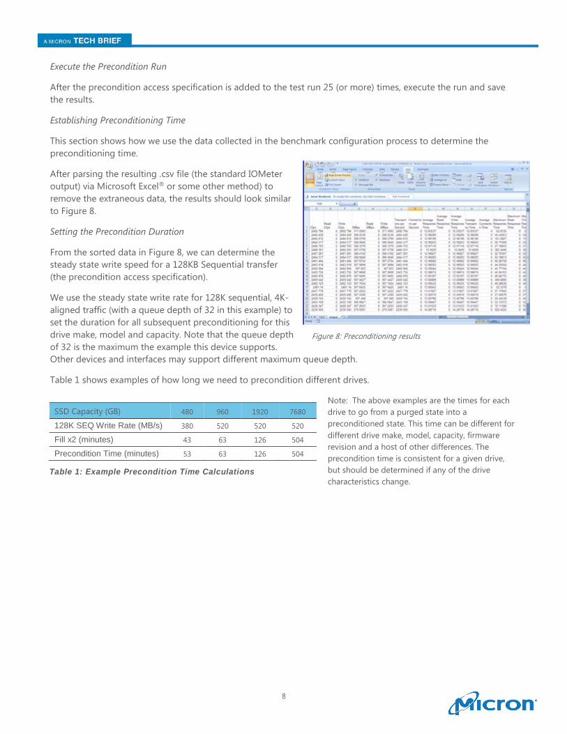
After parsing the resulting .csv file (the standard IOMeter output) via Microsoft Excel® or some other method) to remove the extraneous data, the results should look similar to Figure 8.

Setting the Precondition Duration

From the sorted data in Figure 8, we can determine the steady state write speed for a 128KB Sequential transfer (the precondition access specification).

We use the steady state write rate for 128K sequential, 4K-aligned traffic (with a queue depth of 32 in this example) to set the duration for all subsequent preconditioning for this drive make, model and capacity. Note that the queue depth of 32 is the maximum the example this device supports. Other devices and interfaces may support different maximum queue depth.

Table 1 shows examples of how long we need to precondition different drives.

Note: The above examples are the times for each drive to go from a purged state into a preconditioned state. This time can be different for different drive make, model, capacity, firmware revision and a host of other differences. The precondition time is consistent for a given drive, but should be determined if any of the drive characteristics change.

Figure 8: Preconditioning results

SSD Capacity (GB) 480 960 1920 7680

128K SEQ Write Rate (MB/s) 380 520 520 520

Fill x2 (minutes) 43 63 126 504

Precondition Time (minutes) 53 63 126 504

Table 1: Example Precondition Time Calculations

9

Set Up the Test Metric of Interest

With the precondition access specification and duration established, we can now set up the access specification for each metric of interest. Note that the test flow is similar to previous steps, with only a few differences. For example, supposed we want to measure 4KiB random, 100% write performance. We need to set up an access specification to measure this. As before, we’ll use an example SSD with a maximum queue depth of 32 (see Figures 9, 10 and 11).

1. Set the transfer size to 4K and the percent random/sequential to 100% random.

2. Set the percent read/write distribution slider to 100% write.

3. Align all I/Os to 4K.

4. Set the run time to five minutes and the queue depth to the desired value for the test. (We typically do not vary the queue depth for single-stimulus saturation testing. It is possible to configure a test to vary the queue depth, but IOMeter requires the use of an external scripting tool the use of which is beyond the scope of this document).

Figure 9: Set access specifications for selected metric

Figure 10: Set run time queue depth

10

Note: The total time to reach steady state performance for small block random write traffic may vary. Larger, slower drives may reach steady state more slowly while smaller, faster drives may do so more quickly.

We execute the test, parse the results and plot them as shown in Figure 12. In our example, steady state is achieved after about 50 minutes of run time.

The best way to determine how many times to add the access specification is by testing. The next section shows how to use test data to determine whether the test specification was run enough times for the drive to reach steady state.

Host Configuration May Affect Results

When testing SSD performance, the system configuration on which the test is run may affect results. This section describes two different SSD/host configurations and shows an example of different performance results obtained from each.

We will use the same Enterprise SSD whose 4K random write IOPS are shown in Figure 12.

When we test any SSD, we have several options for system configuration and SSD attachment. We can, for example, use a single or dual processor platform (populating one or both processors), different platform designs and different SSD-to-host connections. We can connect our example SSD to an integrated port or an accessory controller, which could then be connected to a port expander. There are a myriad of choices.

5 30 55 80 105 130 155 180 205 230

IOPS

Test Time (minutes)

4K Random Write

Figure 12: 4K random write Enterprise SSD sample

11

To examine how system configuration can affect performance results, we configured two test systems and measured several IOPS and MB/s performance metrics using the same SSD:

• 4K random 100% write

• 8K random 67% read/33% write

• 64K sequential write

These I/O profiles are used for illustration purposes. Other I/O profiles should show similar results but, as with any performance measurement, each should be validated.

We used two different systems. We connected the same SSD directly to an integrated controller port on one and to an accessory HBA on the other.

In Figure 13, we’ve added a second set of IOPS performance data to what was shown in Figure 12. In Figure 13 (and the other figures in this section), IOPS are shown on the vertical axis and test time along the horizontal axis. Configuration A is in blue; Configuration B is in orange.

The test process we used to generate the data shown in Figure 13 was identical for both configurations and followed the process documented in this paper.

The most obvious difference is that Configuration B is incapable of generating the IOPS performance data of which Configuration A is capable (using the same SSD and the same test process).

Note that IOPS vs. time for Configuration A shows a familiar falloff (as the SSD is written), but the same plot for Configuration B shows none. Further, the IOPS performance for Configuration A is much higher than B at all points during the test.

5 30 55 80 105 130 155 180 205 230

IOPS

Test Time (minutes)

4K Random Write

Configuration A Configuration B

Figure 13: 4K random write Enterprise SSD two configuration sample

5 30 55 80 105 130 155 180 205 230

IOPS

Test Time (minutes)

8K Random 67% Read / 33% WriteConfiguration A Configuration B

Figure 14: 8K Random IOPS Configuration Differences

12

This suggests that Configuration B is incapable of generating enough I/O traffic to show the SSD’s maximum IOPS performance. Configuration A, on the other hand, is capable of doing so. In this case, the performance of Configuration B is being bottlenecked by the system.

Small random 100% read IOPS traffic isn’t the only test metric that may show the differences in host configurations. We also measured 8K random 67% read/33% write and show the results in Figure 14.

Here we see a similar trend: Configuration A measured consistently higher IOPS and showed the expected shape of its IOPS vs. time plot. Configuration B is flat and consistently lower during the test.

As we saw in Figure 13, these results indicate that Configuration B may be incapable of generating enough I/O traffic to show the SSD’s maximum IOPS performance.

Finally, we see a similar pattern for sequential I/O as well.

In Figure 15, Configuration B again is consistently lower than Configuration A, suggesting that Configuration B may not be capable of generating enough I/O traffic to show the SSD’s maximum MB/s (we expect to see flat MB/s vs. time plots for large sequential write traffic, so both lines are the expected shape). Test time for the sequential I/O is shorter, which is also expected because SSDs tend to reach steady state more quickly with a sequential I/O test.

5 20 35 50 65 80 95 110 125

MB/

s

Test Time (minutes)

64K Sequential Write

Configuration A Configuration B

Figure 15: 64K Sequential IOPS Configuration Differences

13

Workflow Review

We can use this same test process to measure single-stimulus performance for any metric of interest. When we want to measure several different stimuli, it is imperative that we follow the same workflow shown in Figure 16.

Why Return the SSD to FOB? Stimulus-Sequence Variant Performance Throughout this brief, we’ve asserted that returning the SSD to the FOB state for each test is key to precise, consistent performance measurement. In this section we will show an example where not doing this (and simply changing the order in which the stimuli are applied) can give vastly different results.

We’ll see how the test sequence: 4K random write, 128K sequential write, 4K random write produces very different results than the reverse sequence of 128K sequential write, 4K random write, 128K sequential write.

The plot in Figure 15 shows steady state performance for an example SSD when we apply the stimulus sequence (each stimulus is applied until the drive reaches steady state). The IOPS performance for each is shown on the y-axis for each sequence.

First sequence 1. 4K random 100% write 2. 128K sequential 100% write 3. 4K random 100% write

Second sequence 1. 128K sequential 100% write 2. 4K random 100% write 4. 128K sequential 100% write

Figure 16: Test process for multiple stimuli

14

First sequence: As expected, the IOPS performance for the 128K sequential write is lower than the IOPS for the 4K random write in both test sequences (because each I/O is much larger, there will be fewer intervals). Note that the IOPS performance for each 4K random write interval is consistent. Figure 17 shows the results.

Second sequence: We secure erased the same drive to FOB and applied the second sequence of stimuli (the I/O patterns are simply reversed). Figure 18 shows the results.

Note also that the drive was NOT returned to the FOB state during at any point during either test — each stimulus was applied immediately following the completion of the previous stimulus.

If we assume that we do not need to restore an SSD to FOB before changing stimuli, we would expect that the IOPS performance of the two 128K sequential write intervals in Figure 18 would be the same. However, Figure 18 shows that this is not the case. The IOPS performance of the second 128K sequential write interval, despite being written into steady state, is lower than the first 128K write interval.

In this example, the order in which the stimuli were applied was the only variable, but the measured performance was quite different—this drive clearly demonstrates the write-history sensitivity mentioned at the beginning of this brief. If the drive had been returned to FOB between these tests, this variance would not have been observed, and the accuracy of the test results would have increased.

The Bottom Line Micron’s Enterprise SSD performance measurement technique ensures consistent, repeatable performance measurements relevant to the Enterprise customer. Through a combination of preconditioning and single stimulus testing into steady state, we remove run-to-run and write-history-based performance fluctuation.

Differences in host configuration may affect performance (IOPS, MB/s or latency) results. Some hosts may not be capable of generating sufficient I/O traffic to show the SSD’s maximum IOPS, MB/s or lowest latency. The test method is in alignment with current industry test methods and provides a level playing field for all drives measured.

micron.com This technical marketing brief is published by Micron and has not been authorized, sponsored, or otherwise approved by any other company. Products are warranted only to meet Micron’s production data sheet specifications. Products and specifications are subject to change without notice. ©2011 Micron Technology, Inc. Micron and the Micron logo are trademarks of Micron Technology, Inc. All other trademarks are the property of their respective owners. All rights reserved. Rev. B 4/17, CCMMD-676576390-1721

Figure 17: Random/Sequential/Random stimulus sequence

Figure 18: Sequential/Random/Sequential Stimulus sequence