best practices for oracle spatial on oracle exadata database machine
TRANSCRIPT
May 2011 Oracle Spatial User Conference

Oracle Spatial User Conference!
May 19, 2011 Ronald Reagan Building and International Trade Center
Washington, DC USA

Daniel Geringer Senior Software Development Manager Oracle’s Spatial Technologies
May 2011 Oracle Spatial User Conference

Best Practices for Oracle Spatial on Oracle Exadata Database Machine
May 2011 Oracle Spatial User Conference

What Is Exadata?

What Is the Oracle Exadata Database Machine?
• Oracle SUN hardware uniquely engineered to work together with Oracle database software
• Key features: • Database Grid – Up to 128 Intel cores connected by 40 Gb/second
InfiniBand fabric, for massive parallel query processing. • Raw Disk – Up to 336 TB of uncompressed storage (high
performance or high capacity) • Memory – Up to 2 TB • Exadata Hybrid Columnar Compression (EHCC) – Query and
archive modes available. 10x-30x compression. • Storage Servers – Up to 14 storage servers (168 Intel cores) that
can perform massive parallel smart scans. Smart scans offloads SQL predicate filtering to the raw data blocks. Results in much less data transferred, and dramatically improved performance.
• Storage flash cache – Up to 5.3 TB with I/O resource management
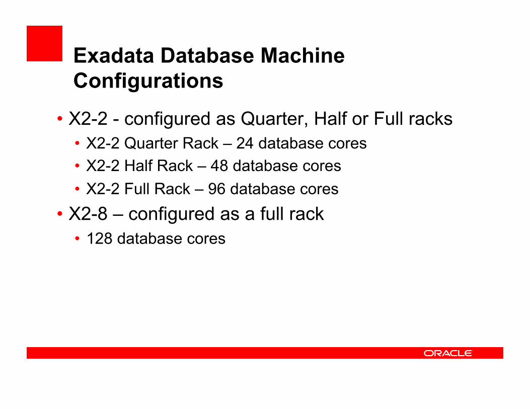
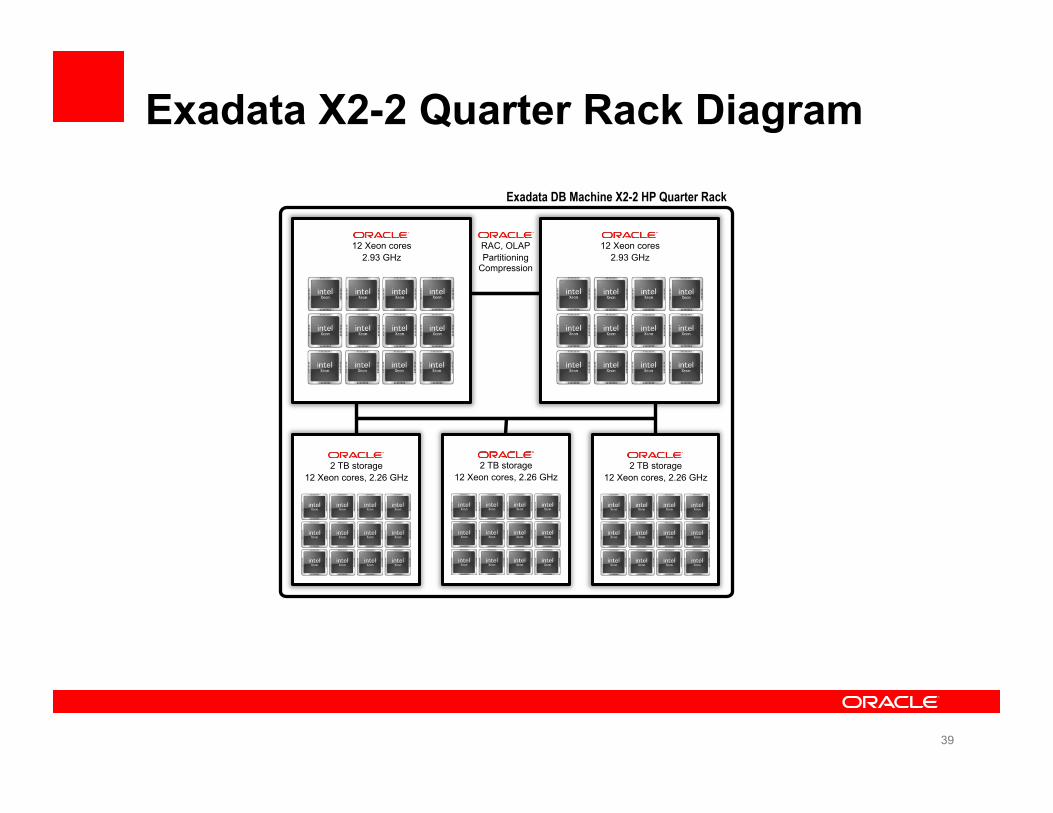
Exadata Database Machine Configurations
• X2-2 - configured as Quarter, Half or Full racks • X2-2 Quarter Rack – 24 database cores • X2-2 Half Rack – 48 database cores • X2-2 Full Rack – 96 database cores
• X2-8 – configured as a full rack • 128 database cores

8
12 Xeon cores 2.93 GHz
12 Xeon cores 2.93 GHz
2 TB storage 12 Xeon cores, 2.26 GHz
2 TB storage 12 Xeon cores, 2.26 GHz
2 TB storage 12 Xeon cores, 2.26 GHz
RAC, OLAP Partitioning
Compression
Exadata DB Machine X2-2 HP Quarter Rack
Exadata X2-2 Quarter Rack Diagram
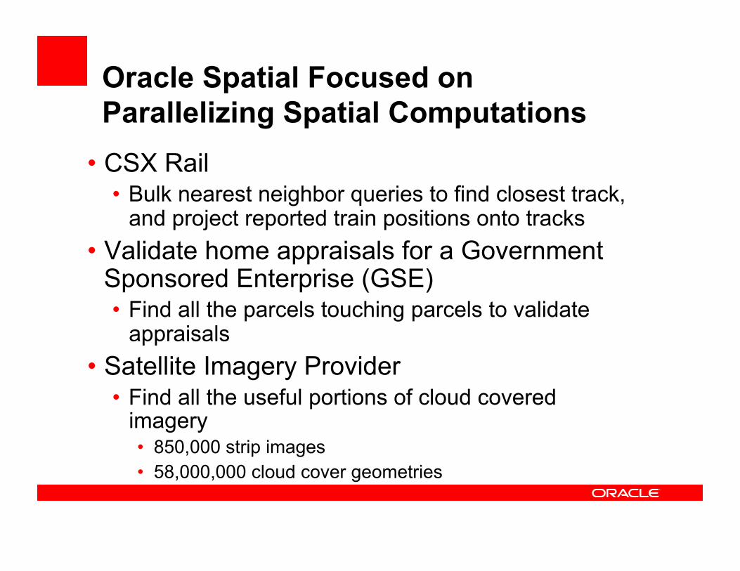
Oracle Spatial Focused on Parallelizing Spatial Computations
• CSX Rail • Bulk nearest neighbor queries to find closest track,
and project reported train positions onto tracks • Validate home appraisals for a Government
Sponsored Enterprise (GSE) • Find all the parcels touching parcels to validate
appraisals • Satellite Imagery Provider
• Find all the useful portions of cloud covered imagery • 850,000 strip images • 58,000,000 cloud cover geometries
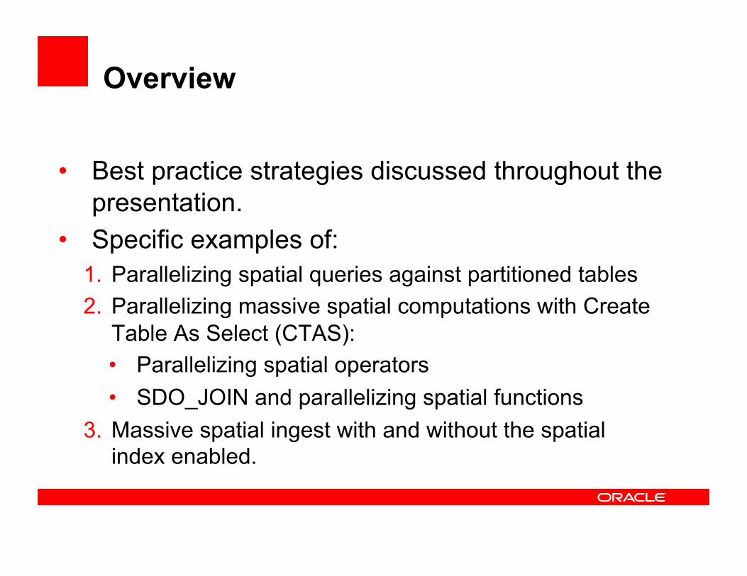
Overview
• Best practice strategies discussed throughout the presentation.
• Specific examples of: 1. Parallelizing spatial queries against partitioned tables 2. Parallelizing massive spatial computations with Create
Table As Select (CTAS): • Parallelizing spatial operators • SDO_JOIN and parallelizing spatial functions
3. Massive spatial ingest with and without the spatial index enabled.

Parallelizing Spatial Queries Against Partitioned Tables
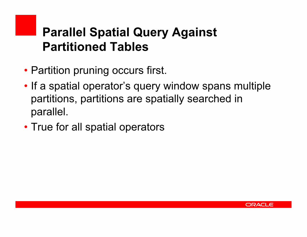
Parallel Spatial Query Against Partitioned Tables
• Partition pruning occurs first. • If a spatial operator’s query window spans multiple
partitions, partitions are spatially searched in parallel.
• True for all spatial operators
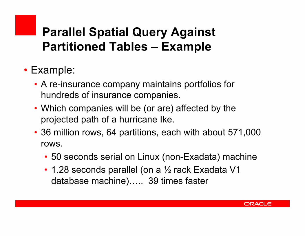
Parallel Spatial Query Against Partitioned Tables – Example
• Example: • A re-insurance company maintains portfolios for
hundreds of insurance companies. • Which companies will be (or are) affected by the
projected path of a hurricane Ike. • 36 million rows, 64 partitions, each with about 571,000
rows. • 50 seconds serial on Linux (non-Exadata) machine • 1.28 seconds parallel (on a ½ rack Exadata V1
database machine)….. 39 times faster

Spatial Operators Can Parallelize with Create Table As Select (CTAS)
Parallel and CTAS With Spatial Operators
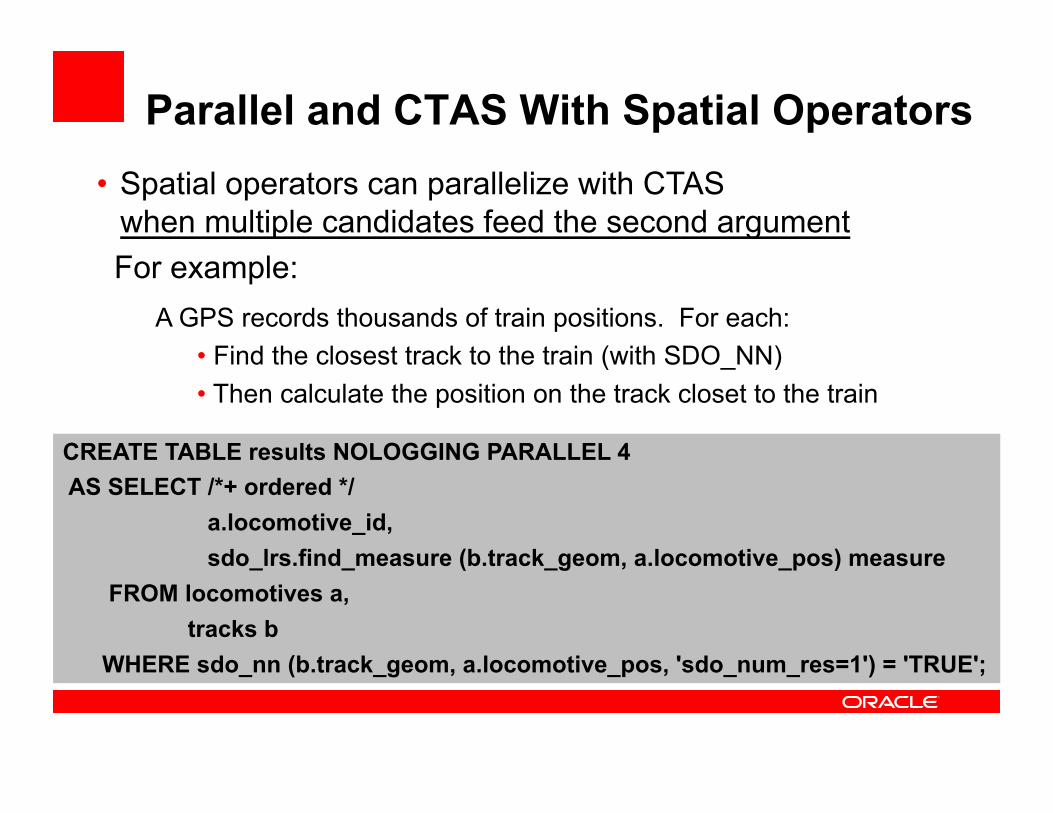
CREATE TABLE results NOLOGGING PARALLEL 4 AS SELECT /*+ ordered */ a.locomotive_id, sdo_lrs.find_measure (b.track_geom, a.locomotive_pos) measure FROM locomotives a, tracks b WHERE sdo_nn (b.track_geom, a.locomotive_pos, 'sdo_num_res=1') = 'TRUE';
• Spatial operators can parallelize with CTAS when multiple candidates feed the second argument
For example: A GPS records thousands of train positions. For each:
• Find the closest track to the train (with SDO_NN) • Then calculate the position on the track closet to the train
Parallel and CTAS With Spatial Operators
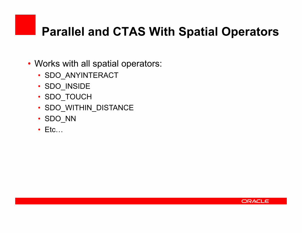
• Works with all spatial operators: • SDO_ANYINTERACT • SDO_INSIDE • SDO_TOUCH • SDO_WITHIN_DISTANCE • SDO_NN • Etc…
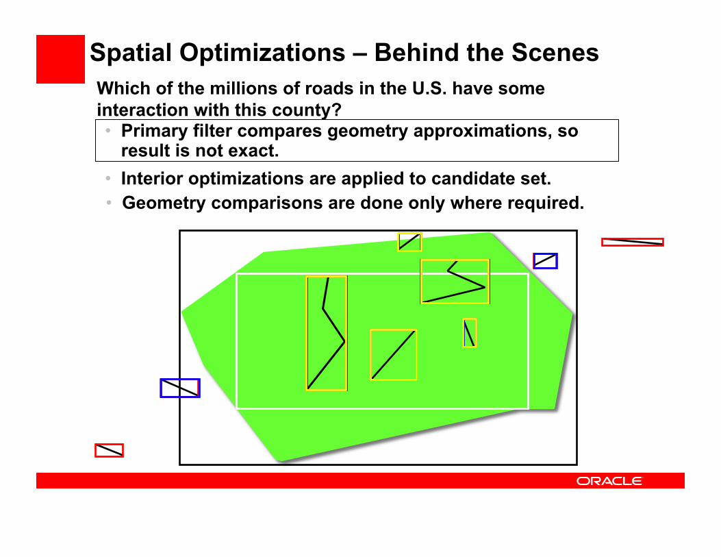
Spatial Optimizations – Behind the Scenes Which of the millions of roads in the U.S. have some interaction with this county? • Primary filter compares geometry approximations, so
result is not exact. • Interior optimizations are applied to candidate set. • Geometry comparisons are done only where required.

Spatial Operators
When possible make the query window a polygon.
The SDO_JOIN Operation
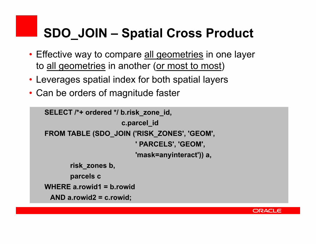
SDO_JOIN – Spatial Cross Product
SELECT /*+ ordered */ b.risk_zone_id, c.parcel_id FROM TABLE (SDO_JOIN ('RISK_ZONES', 'GEOM', ' PARCELS', 'GEOM', 'mask=anyinteract')) a, risk_zones b, parcels c WHERE a.rowid1 = b.rowid AND a.rowid2 = c.rowid;
• Effective way to compare all geometries in one layer to all geometries in another (or most to most)
• Leverages spatial index for both spatial layers • Can be orders of magnitude faster

SDO_JOIN – When is it Most Effective? • If one of the layers is a polygon layer:
• When not many geometries are associated with each polygon, SDO_JOIN may be much more effective
• When many geometries are associated with each polygon, SDO_ANYINTERACT may be more effective
• SDO_ANYINTERACT performs interior optimization

SDO_JOIN – One More Strategy - Parallel
ALTER SESSION ENABLE PARALLEL DDL; ALTER SESSION ENABLE PARALLEL DML; ALTER SESSION ENABLE PARALLEL QUERY;
CREATE TABLE result1 NOLOGGING PARALLEL 4 AS SELECT a.rowid1 AS risk_zones_rowid, a.rowid2 AS parcels_rowid FROM TABLE ( SDO_JOIN ('RISK_ZONES', 'GEOM', ' PARCELS', 'GEOM') );
• First parallelize SDO_JOIN, primary filter only
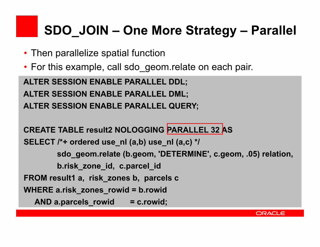
SDO_JOIN – One More Strategy – Parallel
ALTER SESSION ENABLE PARALLEL DDL; ALTER SESSION ENABLE PARALLEL DML; ALTER SESSION ENABLE PARALLEL QUERY;
CREATE TABLE result2 NOLOGGING PARALLEL 32 AS SELECT /*+ ordered use_nl (a,b) use_nl (a,c) */ sdo_geom.relate (b.geom, 'DETERMINE', c.geom, .05) relation, b.risk_zone_id, c.parcel_id FROM result1 a, risk_zones b, parcels c WHERE a.risk_zones_rowid = b.rowid AND a.parcels_rowid = c.rowid;
• Then parallelize spatial function • For this example, call sdo_geom.relate on each pair.
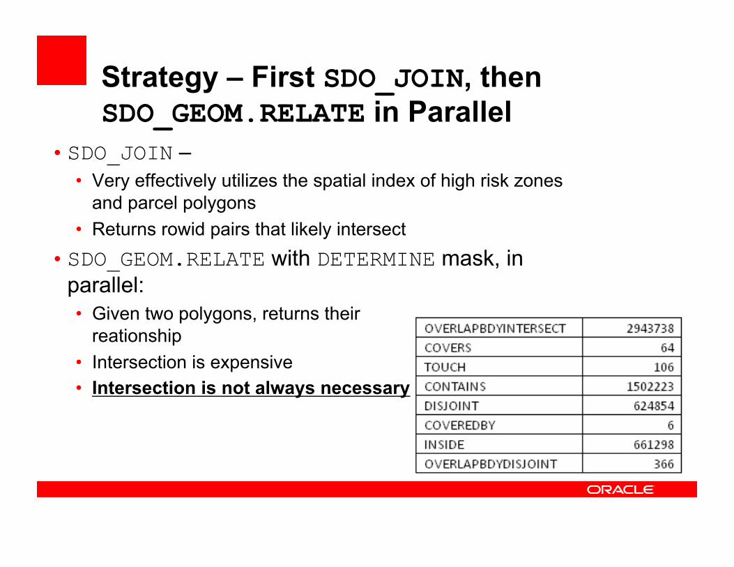
Strategy – First SDO_JOIN, then SDO_GEOM.RELATE in Parallel
• SDO_JOIN – • Very effectively utilizes the spatial index of high risk zones
and parcel polygons • Returns rowid pairs that likely intersect
• SDO_GEOM.RELATE with DETERMINE mask, in parallel: • Given two polygons, returns their
reationship • Intersection is expensive • Intersection is not always necessary

Further Optimizations
• High risk zone INSIDE parcel polygon
• Parcel CONTAINS high risk zone polygon
Strategy – First SDO_JOIN, then SDO_GEOM.RELATE in Parallel
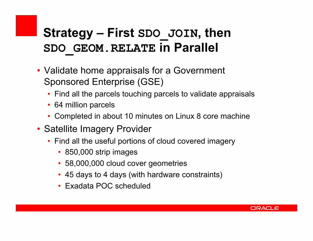
• Validate home appraisals for a Government Sponsored Enterprise (GSE) • Find all the parcels touching parcels to validate appraisals • 64 million parcels • Completed in about 10 minutes on Linux 8 core machine
• Satellite Imagery Provider • Find all the useful portions of cloud covered imagery
• 850,000 strip images • 58,000,000 cloud cover geometries • 45 days to 4 days (with hardware constraints) • Exadata POC scheduled

Massive Spatial Ingest
Local Partitioned Spatial Indexes
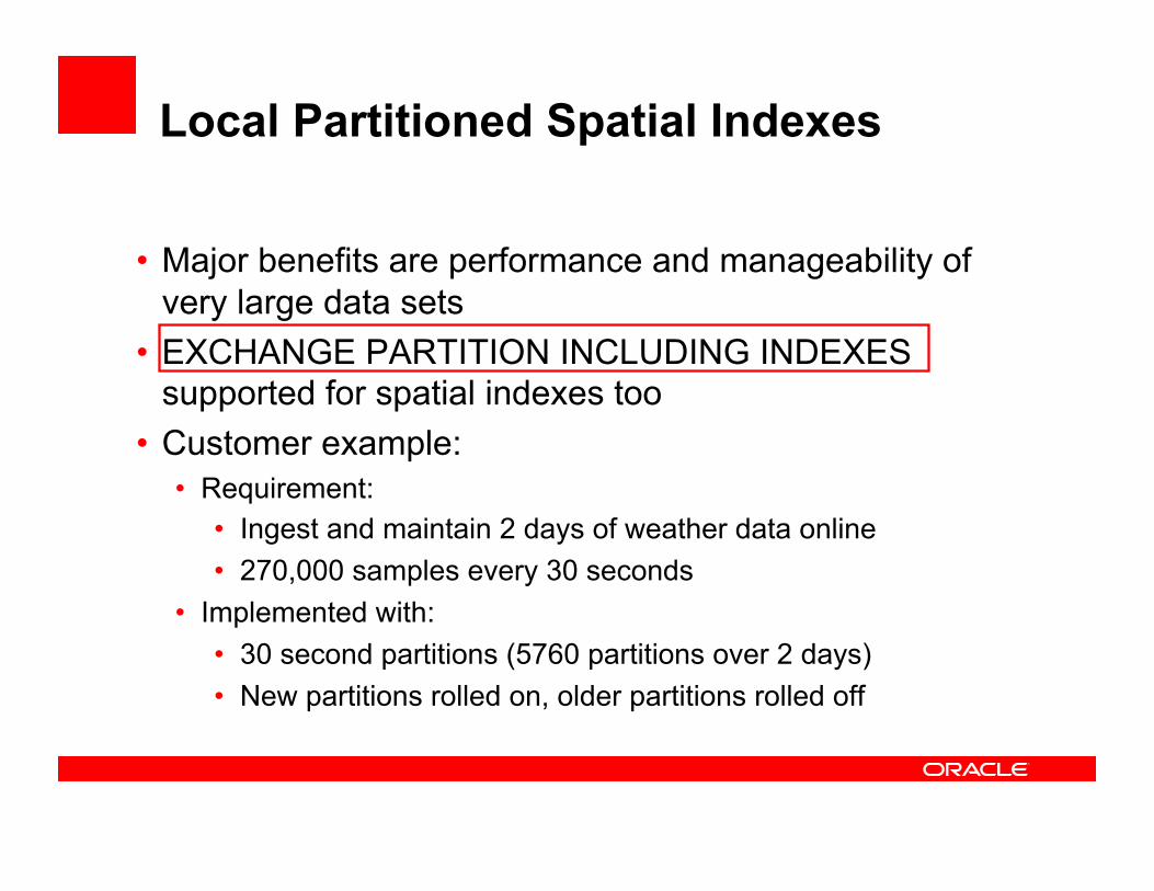
• Major benefits are performance and manageability of very large data sets
• EXCHANGE PARTITION INCLUDING INDEXES supported for spatial indexes too
• Customer example: • Requirement:
• Ingest and maintain 2 days of weather data online • 270,000 samples every 30 seconds
• Implemented with: • 30 second partitions (5760 partitions over 2 days) • New partitions rolled on, older partitions rolled off

Alter Partition Exchange Including Indexes (Spatial Indexes too)
ALTER TABLE weather_data_part EXCHANGE PARTITION p1 WITH TABLE new_weather_data INCLUDING INDEXES WITHOUT VALIDATION;
• Parallel create index (spatial index too) on new_weather_data • Partition P1 is an empty leading partition • Update partitioned table with new weather data in a fraction of a
second. • No need to maintain an index on INSERT.
Alter Partition Exchange With UPDATE GLOBAL INDEXES
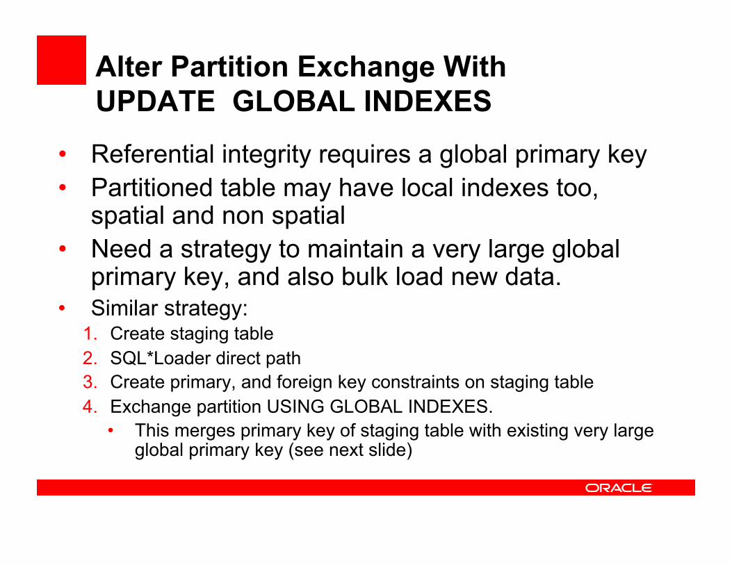
• Referential integrity requires a global primary key • Partitioned table may have local indexes too,
spatial and non spatial • Need a strategy to maintain a very large global
primary key, and also bulk load new data. • Similar strategy:
1. Create staging table 2. SQL*Loader direct path 3. Create primary, and foreign key constraints on staging table 4. Exchange partition USING GLOBAL INDEXES.
• This merges primary key of staging table with existing very large global primary key (see next slide)

Alter Partition Exchange With UPDATE GLOBAL INDEXES (continued)
ALTER TABLE weather_data_part EXCHANGE PARTITION p1 WITH TABLE new_weather_data WITHOUT VALIDATION UPDATE GLOBAL INDEXES ;
Then rebuild unusable local indexes (spatial and non spatial) for the exchanged partition

Recent Exadata POC (X2-2 Half RAC) • Customer had an 8 year back log of spatial data • Referential integrity required (global primary key)
• One month partitions • Disable constraints (including primary key) • Load historical data with SQL*Loader PARALLEL DIRECT
PATH directly into the partitions • Enable constraints
• Need to process new data coming (daily partitions) • Exchange partition USING GLOBAL INDEXES. • This merges primary key of staging table with existing very
large global primary key • 2 week sample – 8 hours vs 5 minutes on Exadata

Massive Spatial Ingest With Spatial Index Enabled

High Ingest Rates – Another Strategy
• For OLTP applications that need to insert into tables with the spatial index enabled
• Eliminate spatial index contention. Not always necessary, but really helps if ingest rate is very high
• To eliminate spatial index contention, partition table by time and process id (composite partition key) • Assign process id’s to Java pool connections • Each connection only writes to the partition with the same process id
• Partitioning is transparent to the SQL developer. • Queries are written against 1 table. • Oracle manages which partitions to search. • Example continued on next slide…
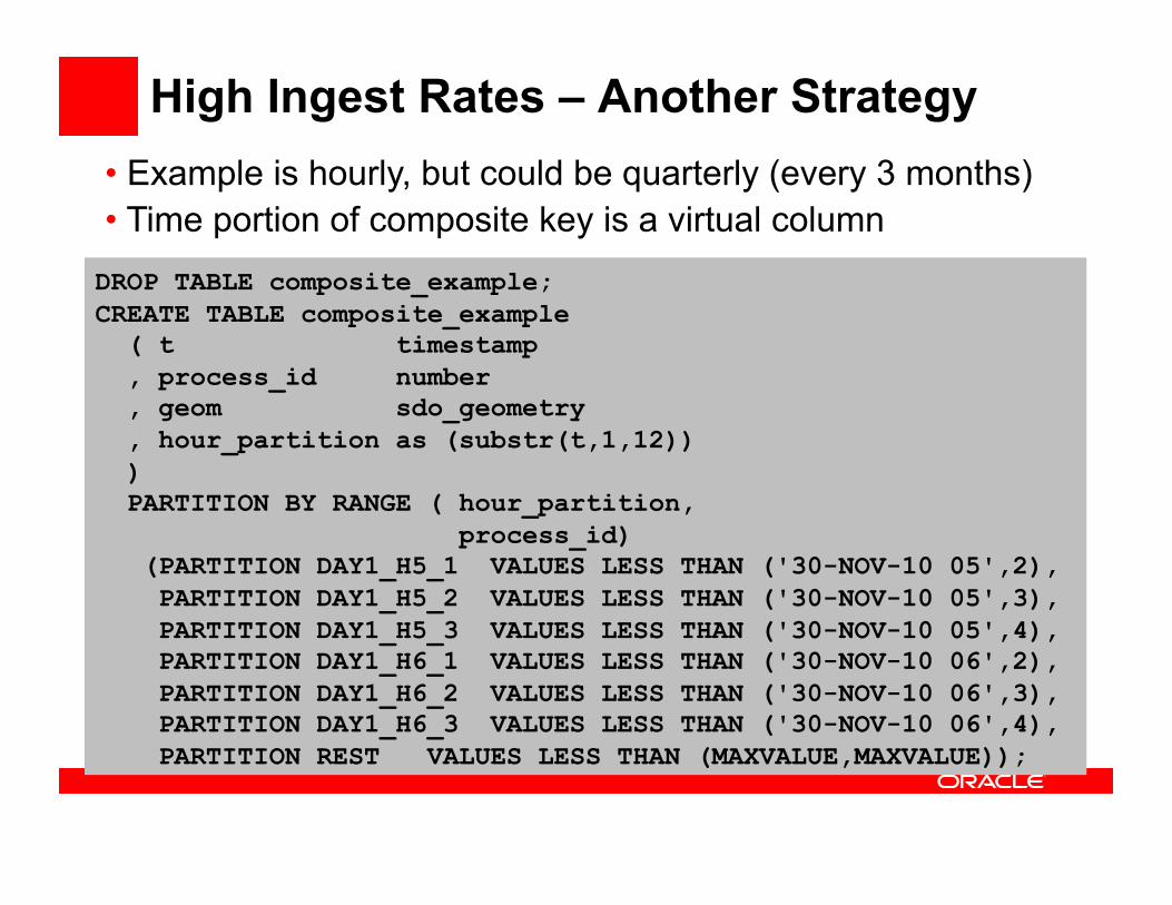
DROP TABLE composite_example; CREATE TABLE composite_example ( t timestamp , process_id number , geom sdo_geometry , hour_partition as (substr(t,1,12)) ) PARTITION BY RANGE ( hour_partition, process_id) (PARTITION DAY1_H5_1 VALUES LESS THAN ('30-NOV-10 05',2), PARTITION DAY1_H5_2 VALUES LESS THAN ('30-NOV-10 05',3), PARTITION DAY1_H5_3 VALUES LESS THAN ('30-NOV-10 05',4), PARTITION DAY1_H6_1 VALUES LESS THAN ('30-NOV-10 06',2), PARTITION DAY1_H6_2 VALUES LESS THAN ('30-NOV-10 06',3), PARTITION DAY1_H6_3 VALUES LESS THAN ('30-NOV-10 06',4), PARTITION REST VALUES LESS THAN (MAXVALUE,MAXVALUE));
High Ingest Rates – Another Strategy • Example is hourly, but could be quarterly (every 3 months) • Time portion of composite key is a virtual column

<Insert Picture Here>
What We Tested

Inserting With Spatial Index Enabled (Implemented These Recommendations)
• For fastest ingest, each partition should be written to by only one writer.
• Batch inserts are critical to performance: • FORALL bulk inserts (if PL/SQL) … benchmark does this • JDBC Update Batching (if Java)
• Set sdo_dml_batch_size = 15000 (this really helps) • Benchmark commits every 15000 inserts
• Increase SGA and Log file sizes • May not be necessary, if resources are not saturated • For benchmark, SGA set to 32 Gb, and each log file to 16 Gb.

How the Benchmark Works
• Data is generated dynamically in PL/SQL • You control the number of parallel processes to run • All processes are clones of each other • Each process gets passed a process id • Each process insets into an exclusive table
(simulating an exclusive partition), for example: • Process 1 inserts into tracks_1 (spatial index enabled) • Process 2 inserts into tracks_2 (spatial index enabled) • Etc.. • All tables start empty with a spatial index enabled
• You can specify on which node in the RAC to run the process, or use the scan listener to decide.
39
12 Xeon cores 2.93 GHz
12 Xeon cores 2.93 GHz
2 TB storage 12 Xeon cores, 2.26 GHz
2 TB storage 12 Xeon cores, 2.26 GHz
2 TB storage 12 Xeon cores, 2.26 GHz
RAC, OLAP Partitioning
Compression
Exadata DB Machine X2-2 HP Quarter Rack
Exadata X2-2 Quarter Rack Diagram

Exadata ¼ RAC Results With Spatial Index Enabled
• Parallel Degree - how many processes are running in parallel • Each process writes to an exclusive table. • 1m/15k means each process inserts 1,000,000 rows and commits every
15000 (with sdo_dml_batch_size=15000) • 8x2 means 16 processes, 8 running on node 1 and 8 on node 2

Exadata ¼ RAC Results
Some Patch Recommendations

Spatial Patch Recommendations • It is always recommended to install the most
recent patch set and check for the latest Oracle Spatial patch information at support.oracle.com
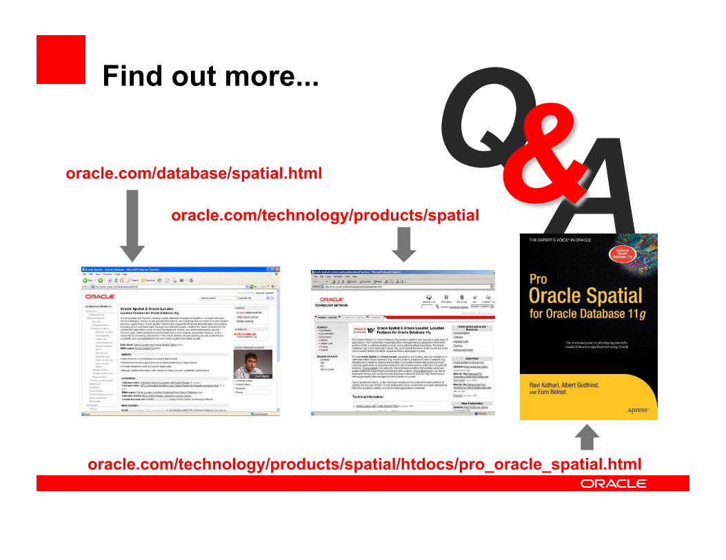
Find out more...
oracle.com/database/spatial.html
oracle.com/technology/products/spatial
oracle.com/technology/products/spatial/htdocs/pro_oracle_spatial.html
AQ

