best practices for a data warehouse on oracle database … · best practices for a data warehouse...

Best practices for a Data Warehouse on Oracle Database 11g

An Oracle White Paper

September 2008

Best Practices for a Data Warehouse on Oracle Database 11g

NOTE:

The following is intended to outline our general product direction. It is intended

for information purposes only, and may not be incorporated into any contract. It is

not a commitment to deliver any material, code, or functionality, and should not be

relied upon in making purchasing decisions. The development, release, and timing

of any features or functionality described for Oracle’s products remains at the sole

discretion of Oracle.



Note:.................................................................................................................... 2 Executive Summary .......................................................................................... 4 Introduction ....................................................................................................... 4 Balanced Configuration.................................................................................... 5

Interconnect .................................................................................................. 6 Disk Layout ................................................................................................... 7

Logical Model .................................................................................................... 9 Physical Model ................................................................................................. 10

Staging layer ................................................................................................. 10 Efficient Data Loading.......................................................................... 11

Foundation layer - Third Normal Form ................................................. 14 Optimizing 3NF ..................................................................................... 15

Access layer - Star Schema ........................................................................ 19 Optimizing Star Queries........................................................................ 20

System Management ....................................................................................... 22 Workload Management.............................................................................. 22 Workload Monitoring ................................................................................ 26 Resource Manager ...................................................................................... 31 Optimizer Statistics Management ............................................................ 32 Initialization Parameter .............................................................................. 34

Memory allocation ................................................................................. 34 Controlling Parallel Execution ............................................................. 36 Enabling efficient IO throughput........................................................ 36 Star Query ............................................................................................... 37

Conclusion........................................................................................................ 37


Best practices for a Data Warehouse on Oracle Database 11g

EXECUTIVE SUMMARY

Increasingly companies are recognizing the value of an enterprise data warehouse

(EDW). A true EDW provides a single 360-degree view of the business and a

powerful platform for a wide spectrum of business intelligence tasks ranging from

predictive analysis to near real-time strategic and tactical decision support

throughout the organization. In order to ensuring the EDW will get the optimal

performance and will scale as your data set grows you need to get three

fundamental things correct, the hardware configuration, the data model and the

data loading process. By designing these three corner stones correctly you can

seamlessly scale out your EDW without having to constantly tune or tweak the

system.

INTRODUCTION

Today’s information architecture is much more dynamic than it was just a few years

ago. Businesses now demand more information sooner and they are delivering

analytics from their EDW to an every-widening set of users and applications than

ever before. In order to keep up with this increase in demand the EDW must now

be near real-time and be highly available. How do you know if your data warehouse

is getting the best possible performance? Or whether you've made the right

decisions to keep your multi-TB system highly available?

Based on over a decade of successful customer data warehouse implementations

this white paper provides a set of best practices and “how-to” examples for

deploying a data warehouse on Oracle Database 11g and leveraging it’s best-of-

breed functionality. The paper is divided into four sections:

The first section deals with the key aspects of configuring your hardware

platform of choice to ensure optimal performance.

The second briefly describes the two fundamental logical models used for

database warehouses.

The third outlines how to implement the physical model for these logical models

in the most optimal manner in an Oracle database.

Finally the fourth section covers system management techniques including

workload management and database configuration.


This paper is by no means a complete guide for Data Warehousing with Oracle.

You should refer to the Oracle Database’s documentation, especially the Oracle

Data Warehouse Guide and the VLDB and Partitioning Guide, for complete

details on all of Oracle’s warehousing features.

BALANCED CONFIGURATION

Regardless of the design or implementation of a data warehouse the initial key to

good performance lies in the hardware configuration used. This has never been

more evident than with the recent increase in the number of Data Warehouse

appliances in the market. Many data warehouse operations are based upon large

tables scans and other IO-intensive operations, which perform vast quantities of

random IOs. In order to achieve optimal performance the hardware configuration

must be sized end to end to sustain this level of throughput. This type of hardware

configuration is called a balanced system. In a balanced system all components -

from the CPU to the disks - are orchestrated to work together to guarantee the

maximum possible IO throughput.

But how do you go about sizing such a system? You must first understand how

much throughput capacity is required for your system and how much throughput

each individual CPU or core in your configuration can drive. Both pieces of

information can be determined from an existing system. However, if no

environment specific values are available, a value of approximately 200MB/sec IO

throughput per core is a good planning number for designing a balanced system.

All subsequent critical components on the IO path - the Host Bus Adapters, fiber

channel connections, the switch, the controller, and the disks – have to be sized

appropriately.

DiskArray 1

DiskArray 2

DiskArray 3

DiskArray 4

DiskArray 5

DiskArray 6

DiskArray 7

DiskArray 8

FC-Switch1 FC-Switch2

HB

A1

HB

A2

HB

A1

HB

A2

HB

A1

HB

A2

HB

A1

HB

A2

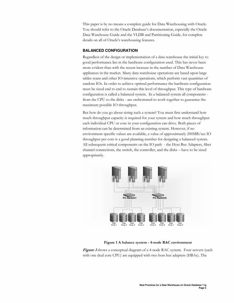
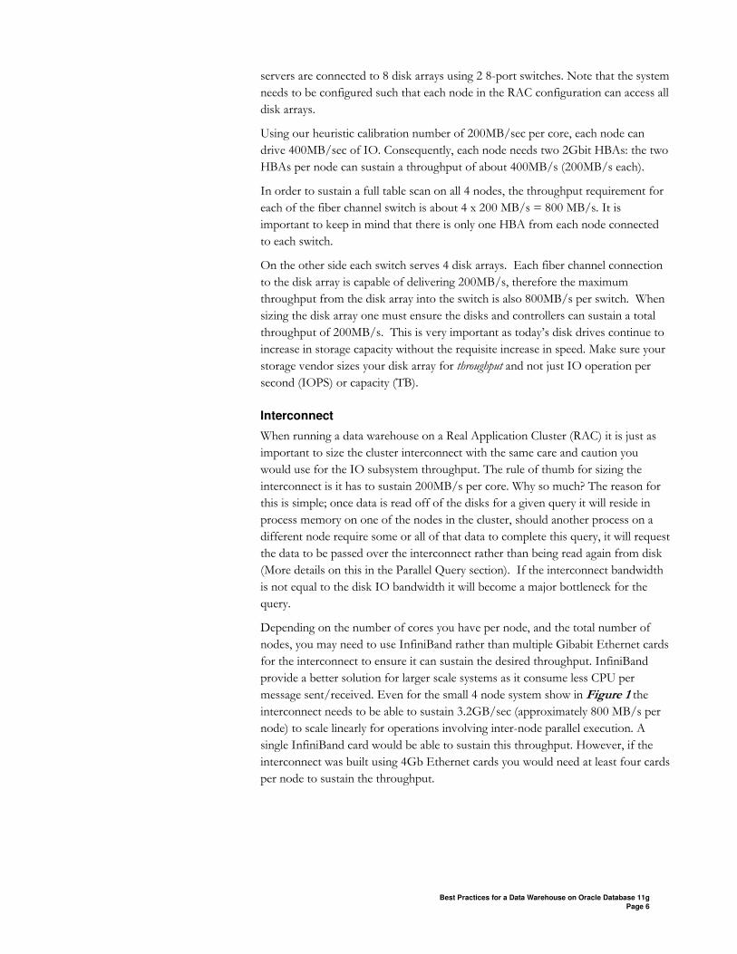
Figure 1 A balance system - 4-node RAC environment

Figure 1 shows a conceptual diagram of a 4-node RAC system. Four servers (each

with one dual core CPU) are equipped with two host bus adapters (HBAs). The


servers are connected to 8 disk arrays using 2 8-port switches. Note that the system

needs to be configured such that each node in the RAC configuration can access all

disk arrays.

Using our heuristic calibration number of 200MB/sec per core, each node can

drive 400MB/sec of IO. Consequently, each node needs two 2Gbit HBAs: the two

HBAs per node can sustain a throughput of about 400MB/s (200MB/s each).

In order to sustain a full table scan on all 4 nodes, the throughput requirement for

each of the fiber channel switch is about 4 x 200 MB/s = 800 MB/s. It is

important to keep in mind that there is only one HBA from each node connected

to each switch.

On the other side each switch serves 4 disk arrays. Each fiber channel connection

to the disk array is capable of delivering 200MB/s, therefore the maximum

throughput from the disk array into the switch is also 800MB/s per switch. When

sizing the disk array one must ensure the disks and controllers can sustain a total

throughput of 200MB/s. This is very important as today’s disk drives continue to

increase in storage capacity without the requisite increase in speed. Make sure your

storage vendor sizes your disk array for throughput and not just IO operation per

second (IOPS) or capacity (TB).

Interconnect

When running a data warehouse on a Real Application Cluster (RAC) it is just as

important to size the cluster interconnect with the same care and caution you

would use for the IO subsystem throughput. The rule of thumb for sizing the

interconnect is it has to sustain 200MB/s per core. Why so much? The reason for

this is simple; once data is read off of the disks for a given query it will reside in

process memory on one of the nodes in the cluster, should another process on a

different node require some or all of that data to complete this query, it will request

the data to be passed over the interconnect rather than being read again from disk

(More details on this in the Parallel Query section). If the interconnect bandwidth

is not equal to the disk IO bandwidth it will become a major bottleneck for the

query.

Depending on the number of cores you have per node, and the total number of

nodes, you may need to use InfiniBand rather than multiple Gibabit Ethernet cards

for the interconnect to ensure it can sustain the desired throughput. InfiniBand

provide a better solution for larger scale systems as it consume less CPU per

message sent/received. Even for the small 4 node system show in Figure 1 the

interconnect needs to be able to sustain 3.2GB/sec (approximately 800 MB/s per

node) to scale linearly for operations involving inter-node parallel execution. A

single InfiniBand card would be able to sustain this throughput. However, if the

interconnect was built using 4Gb Ethernet cards you would need at least four cards

per node to sustain the throughput.


Disk Layout

Once you have confirmed the hardware configuration has been set up as a balanced

system that can sustain your required throughput you need to focus on your disk

layout. One of the key problems we see with existing data warehouse

implementations today is poor disk design. Often times we will see a large

Enterprise Data Warehouse (EDW) residing on the same disk array as one or more

other applications. This is often done because the EDW does not generate the

number of IOPS to saturate the disk array. What is not taken into consideration in

these situations is the fact that the EDW will do fewer, larger IOs, which will easily

exceed the disk arrays throughput capabilities in terms of gigabytes per second.

Ideally you want your data warehouse to reside on its own storage array(s).

When configuring the storage subsystem for a data warehouse it should be simple,

efficient, highly available and very scalable. It should not be complicated or hard to

scale out. One of the easiest ways to achieve this is to apply the S.A.M.E.

methodology (Stripe and Mirror Everything). S.A.M.E. can be implemented at the

hardware level or by using ASM (Automatic Storage Management – a capability 1st

introduced in Oracle Database 10g) or by using a combination of both. This paper

will only deal with implementing S.A.M.E using a combination of hardware and

ASM features.

From the hardware perspective, build redundancy in by implementing mirroring at

the storage subsystem level using RAID 1. Once the RAID groups have been

create you can turn them over to ASM. ASM provides filesystem and volume

manager capabilities, built into the Oracle Database kernel. To use ASM for

database storage, you must first create an ASM instance. Once the ASM instance is

started, you can create your ASM disk groups. A disk group is a set of disk devices,

which ASM manages as a single unit. A disk group is comparable to a LVM’s

(Logical Volume Manager) volume group or a storage group. Each disk in the disk

group should have the same physical characteristics including size and speed, as

ASM spreads data evenly across all of the devices in the disk group to optimize

performance and utilization. If the devices of a single disk group have different

physical characteristic it is possible to create artificial hotspots or bottlenecks, so it

is important to always use similar devices in a disk group. ASM uses a 1MB stripe

size by default.

ASM increases database availability by providing the ability to add or remove disk

devices from disk groups without shutting down the ASM instance or the database

that uses it. ASM automatically rebalances the data (files) across the disk group

after disks have been added or removed. This capability allows you to seamlessly

scale out your data warehouse.

For a data warehouse environment a minimum of two ASM diskgroups are

recommend, one for data (DATA) and one for the Flash Recover Area (FRA). For

the sake of simplicity the following example will only focus on creating the DATA

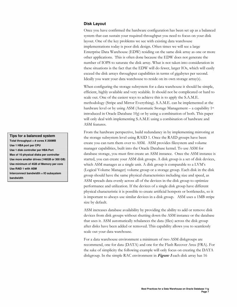
diskgroup. In the simple RAC environment in Figure 1 each disk array has 16

Tips for a balanced system

Total throughput = # cores X 200MB

Use 1 HBA port per CPU

Use 1 disk controller per HBA Port

Max of 10 physical disks per controller

Use more smaller drives (146GB or 300 GB)

Use minimum of 4GB of Memory per core

Use RAID 1 with ASM

Interconnect bandwidth = IO subsystem

bandwidth


physical disks. From these 16 disks, eight RAID 1 groups will be created (see

Figure 2).

LUN A1 LUN A2 LUN A3 LUN A4

LUN A5 LUN A6 LUN A7 LUN A8

Disk12

Disk8

Disk16

Disk4

Disk11

Disk7

Disk15

Disk3

Disk10

Disk6

Disk14

Disk2

Disk9

Disk5

Disk13

Disk1

Figure 2 Eight Raid 1 groups are created from the 16 rawdisks

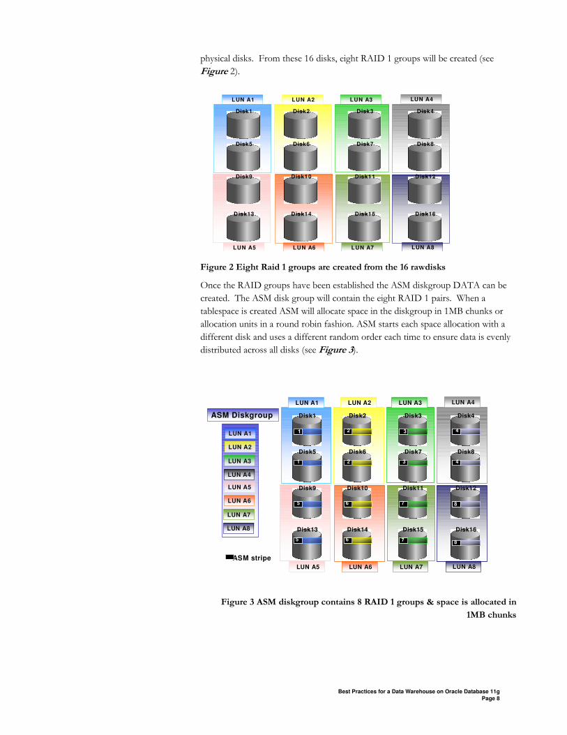
Once the RAID groups have been established the ASM diskgroup DATA can be

created. The ASM disk group will contain the eight RAID 1 pairs. When a

tablespace is created ASM will allocate space in the diskgroup in 1MB chunks or

allocation units in a round robin fashion. ASM starts each space allocation with a

different disk and uses a different random order each time to ensure data is evenly

distributed across all disks (see Figure 3).

LUN A1 LUN A2LUN A2 LUN A3LUN A3 LUN A4LUN A4

LUN A5LUN A5 LUN A6LUN A6 LUN A7LUN A7 LUN A8LUN A8

Disk12Disk12

Disk8Disk8

Disk16Disk16

Disk4Disk4

Disk11Disk11

Disk7Disk7

Disk15Disk15

Disk3Disk3

Disk10Disk10

Disk6Disk6

Disk14Disk14

Disk2Disk2

Disk9Disk9

Disk5Disk5

Disk13Disk13

Disk1Disk1

ASM stripe

11 2 3 4

5 6 7 8

8

1 2 3 4

5 6 77

ASM Diskgroup

LUN A1LUN A1

LUN A2LUN A2

LUN A3LUN A3

LUN A4LUN A4

LUN A5LUN A5

LUN A6LUN A6

LUN A7LUN A7

LUN A8LUN A8

Figure 3 ASM diskgroup contains 8 RAID 1 groups & space is allocated in

1MB chunks


LOGICAL MODEL

The distinction between a logical model and a physical model is sometimes

confusing. In this paper a logical model for a data warehouse will be treated more

as a conceptual or abstract model, a more ideological view of what the data

warehouse should be. The physical model will describe how the data warehouse is

actually built in an Oracle database.

A logical model is an essential part of the development process for a data

warehouse. It allows you to define the types of information needed in the data

warehouse to answer the business questions and the logical relationships between

different parts of the information. It should be simple, easily understood and have

no regard for the physical database, the hardware that will be used to run the

system or the tools that end users will use to access it.

There are two classic models used for data warehouse, Third Normal Form and

dimensional or Star Schema.

Third Normal Form (3NF) is a classical relational-database modelling technique

that minimizes data redundancy through normalization. A 3NF schema is a neutral

schema design independent of any application, and typically has a large number of

tables. It preserves a detailed record of each transaction without any data

redundancy and allows for rich encoding of attributes and all relationships between

data elements. Users typically require a solid understanding of the data in order to

navigate the more elaborate structure reliably.

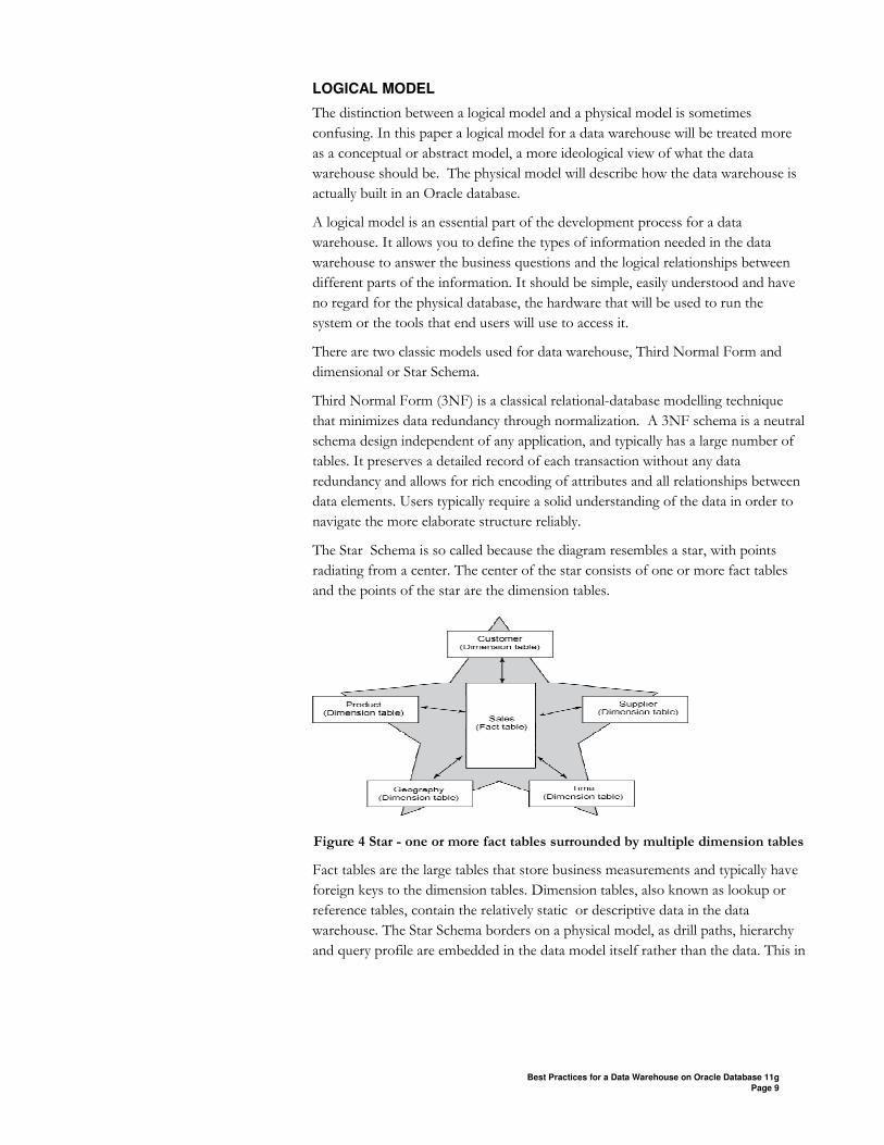
The Star Schema is so called because the diagram resembles a star, with points

radiating from a center. The center of the star consists of one or more fact tables

and the points of the star are the dimension tables.

Figure 4 Star - one or more fact tables surrounded by multiple dimension tables

Fact tables are the large tables that store business measurements and typically have

foreign keys to the dimension tables. Dimension tables, also known as lookup or

reference tables, contain the relatively static or descriptive data in the data

warehouse. The Star Schema borders on a physical model, as drill paths, hierarchy

and query profile are embedded in the data model itself rather than the data. This in


part at least, this is what makes navigation of the model so straightforward for end

users.

There is often much discussion regarding the ‘best’ modeling approach to take for

any given Data Warehouse with each style, classic 3NF or dimensional having their

own strengths and weaknesses. It is likely that Next Generation Data Warehouses

will need to do more to embrace the benefits of each model type rather than rely on

just one - this is the approach that Oracle adopt in our Data Warehouse Reference

Architecture. This is also true of the majority of our customers who use a mixture

of both model forms. Most important is for you to design your model according to

your specific business needs.

PHYSICAL MODEL

The starting point for the physical model is the logical model. The physical model

should mirror the logical model as much as possible, although some changes in the

structure of the tables and / or columns may be necessary. In addition the physical

model will include staging or maintance tables that are usually not included in the

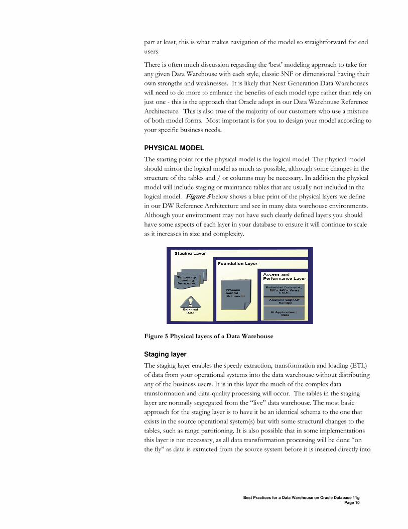
logical model. Figure 5 below shows a blue print of the physical layers we define

in our DW Reference Architecture and see in many data warehouse environments.

Although your environment may not have such clearly defined layers you should

have some aspects of each layer in your database to ensure it will continue to scale

as it increases in size and complexity.

Figure 5 Physical layers of a Data Warehouse

Staging layer

The staging layer enables the speedy extraction, transformation and loading (ETL)

of data from your operational systems into the data warehouse without distributing

any of the business users. It is in this layer the much of the complex data

transformation and data-quality processing will occur. The tables in the staging

layer are normally segregated from the “live” data warehouse. The most basic

approach for the staging layer is to have it be an identical schema to the one that

exists in the source operational system(s) but with some structural changes to the

tables, such as range partitioning. It is also possible that in some implementations

this layer is not necessary, as all data transformation processing will be done “on

the fly” as data is extracted from the source system before it is inserted directly into


the Foundation Layer. Either way you will still have to load data into the

warehouse.

Efficient Data Loading

Whether you are loading into a stage layer or directly into the foundation layer the

goal should be the same, get the data into the warehouse in the most efficient and

expedient manner. Oracle offers several data loading options

• External table or SQL*Loader

• Oracle Data Pump (import & export)

• Change Data Capture or Oracle streams for trickle feeds

• Oracle Transparent Gateways

Which approach should you take? Obviously this will depend on the source and

format of the data you receive. In this paper we will deal with the loading of data

from flat files. If you are loading from flat files into Oracle you have two options,

SQL*Loader or external tables. We strongly recommend that you load using

external tables rather than SQL*Loader. When SQL*Loader is used to load data in

parallel, the data is loaded into temporary extents, only when the transaction is

committed are the temporary extents merged into the actual table. Any existing

space in partially full extents in the table will be skipped. For highly partitioned

tables this could potentially lead to a lot of wasted space.

External Tables

Oracle’s most sophisticated approach to loading flat files is through the use of

external tables. An external table allows you to access data in external sources (flat

file) as if it were in a table in the database. This means that external files can be

queried directly and in parallel using the full power of SQL, PL/SQL, and Java. An

external table is created using the standard create table syntax except it requires an

additional clause. The following SQL command creates an external table for the flat

file ‘sales_data_for_january.dat’.

CREATE TABLE ext_tab_for_sales_data (

Price NUMBER(6),

Quantity NUMBER(6),

Time_id DATE,

Cust_id NUMBER(12),

Prod_id NUMBER(12))

ORGANIZATION EXTERNAL

(TYPE oracle_loader

DEFAULT DIRECTORY admin

ACCESS PARAMETERS


( RECORDS DELIMITED BY newline

BADFILE 'ulcase1.bad'

LOGFILE 'ulcase1.log'

FIELDS TERMINATED BY ","

(Price INTEGER EXTERNAL(6),

Qunantity INTEGER EXTERNAL(6),

Time_id DATE)

LOCATION (sales_data_for_january.dat))

REJECT LIMIT UNLIMITED;

The most common approach when loading data from an external table is to do a

Create Table As Select (CTAS) statement or an Insert As Select (IAS) statement

into an existing table. For example the simple SQL statement below will insert all of

the rows in a flat file into partition p2 of the Sales fact table.

Insert into Sales partition(p2)

Select * From ext_tab_for_sales_data;

Direct Path Load

The key to good load performance is to use direct path load wherever possible. A

direct path load parses the input data according to the description given in the

external table definition, converts the data for each input field to its corresponding

Oracle column data type, and builds a column array structure. These column array

structures are then used to format Oracle data blocks and build index keys. The

newly formatted database blocks are then written directly to the database (multiple

blocks per I/O request using asynchronous writes if the host platform supports

asynchronous I/O) bypassing the database buffer cache.

A CTAS will always use direct path load but an IAS statement will not. In order to

achieve direct path load with an IAS you must add the APPEND hint to the

command.

Insert /*+ APPEND */ into Sales partition(p2)

Select * From ext_tab_for_sales_data;

Direct path loads can also run in parallel. You can set the parallel degree for a

direct path load either by adding the PARALLEL hint to the CTAS or IAS

statement or by setting the PARALLEL clause on both the external table and the

table into which the data will be loaded. Once the parallel degree has been set a

CTAS will automatically do direct path load in parallel but an IAS will not. In

order to enable an IAS to do direct path load in parallel you must alter the session

to enable parallel DML.

ALTER SESSION ENABLE PARALLEL DML;


Insert /*+ APPEND */ into Sales partition(p2)

Select * from ext_tab_for_sales_data;

Partition exchange loads

It is strongly recommended that the larger tables or fact tables in a data warehouse

should be partitioned. One of the great features about partitioning is the ability to

load data quickly and easily with minimal impact on the business users by using the

exchange partition command. The exchange partition command allows you to swap

the data in a non-partitioned table into a particular partition in your partitioned

table. The command does not physically move data it simply updates the data

dictionary to reset a pointer from the partition to the table and vice versa. Because

there is no physical movement of data, this exchange does not generate redo and

undo, making it a sub-second operation and far less likely to impact performance

than any traditional data-movement approaches such as INSERT.

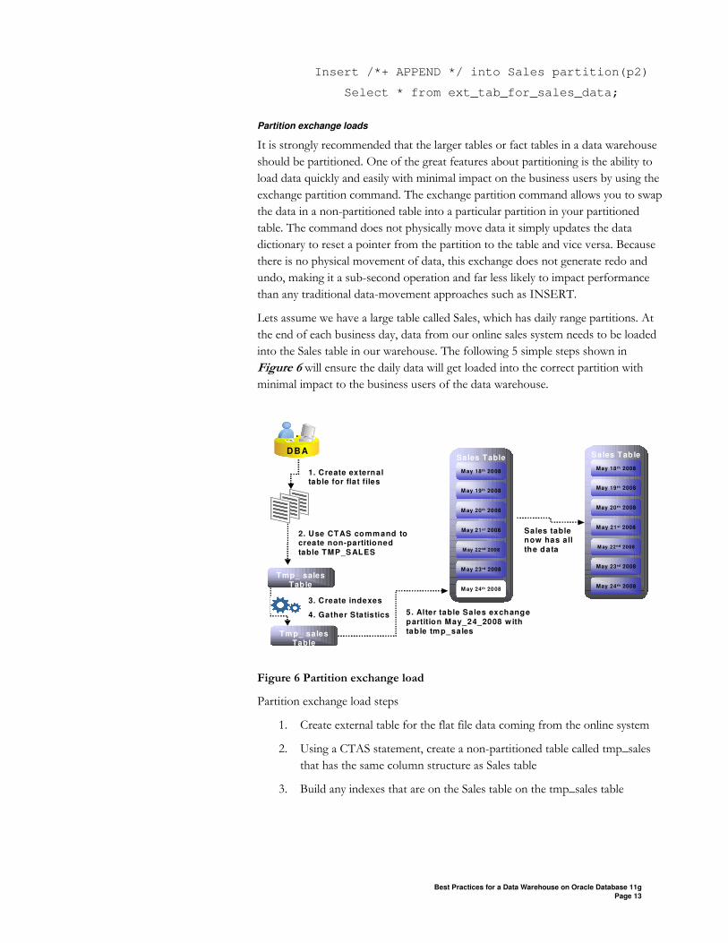
Lets assume we have a large table called Sales, which has daily range partitions. At

the end of each business day, data from our online sales system needs to be loaded

into the Sales table in our warehouse. The following 5 simple steps shown in

Figure 6 will ensure the daily data will get loaded into the correct partition with

minimal impact to the business users of the data warehouse.

Sales Table

M ay 22nd 2008

M ay 23 rd 2008

M ay 24 th 2008

M ay 18 th 2008

M ay 19 th 2008

M ay 20 th 2008

May 21st 20082. Use CTAS command to create non-partitioned

table TMP_SALES

DBA

Tmp_ sales Table

1. Create external table for flat files

3. Create indexes

4. Gather Statistics

Tmp_ sales Table

Sales Table

M ay 22nd 2008

May 23 rd 2008

May 24 th 2008

May 18 th 2008

May 19 th 2008

May 20 th 2008

M ay 21st 2008

5. Alter table Sales exchange

partition May_24_2008 w ith

table tmp_sales

Sales table now has all

the data

Figure 6 Partition exchange load

Partition exchange load steps

1. Create external table for the flat file data coming from the online system

2. Using a CTAS statement, create a non-partitioned table called tmp_sales

that has the same column structure as Sales table

3. Build any indexes that are on the Sales table on the tmp_sales table


4. Gather optimizer statistics on the tmp_sales table

5. Issue the exchange partition command

Alter table Sales exchange partition p2 with

table tmp_sales including indexes without

validation;

The exchange partition command in the final step above, swaps over the definitions

of the named partition and the tmp_sales table, so that the data instantaneously

exists in the right place in the partitioned table. Moreover, with the inclusion of the

two optional extra clauses, index definitions will be swapped and Oracle will not

check whether the data actually belongs in the partition - so the exchange is very

quick.

Data Compression

Another key decision that you need to make during the load phase is whether or

not to compress your data. Oracle compresses data by eliminating duplicate values

in a database block. Using table compression reduces disk and memory usage, often

resulting in better scale-up performance for read-only operations. Table

compression can also speed up query execution by minimizing the number of

round trips required to retrieve data from the disks.

If possible, consider sorting your data before loading it to achieve the best possible

compression rate. The easiest way to sort incoming data is to load it using an

ORDER BY clause on either your CTAS or IAS statement. You should ORDER

BY a NOT NULL column (ideally non numeric) that has a large number of distinct

values (1,000 to 10,000).

Why would you not choose to compress your data? Prior to Oracle Database 11g,

compression was not suitable for tables or partitions where the data would be

changed or updated frequently, as conventional DML would trigger the block to

become uncompressed. If this is the case, you might want to wait until the data is

stable before compressing it. From Oracle Database 11g onwards the new feature,

OLTP Table Compression allows data to be compressed during all types of data

manipulation operations, including conventional DML such as INSERT and

UPDATE. More information on the OLTP table compression features can be

found in Chapter 18 of the Oracle® Database Administrator's Guide 11g.

Finally the use of compression will add some additional CPU overheadrequires to

compress when loading and decompress during query execution, but the overall

performance gain will easily outweigh the cost of compression. The often dramatic

saving in storage costs is an obvious bonus. Oracle strongly recommends

compressing your data.

Foundation layer - Third Normal Form

From staging, the data will transition into the foundation or integration layer via

another set of ETL processes. It is in this layer data begins to take shape and it is

Tips for the Staging Layer

Use external tables

Load using parallel DML stmts CTAS or IAS

Use data compression

Considering range partitioning fact table to

enable partition exchange loads


not uncommon to have some end-user application access data from this layer

especially if they are time sensitive, as data will become available here before it is

transformed into the dimension / performance layer. Traditionally this layer is

implemented in the Third Normal Form (3NF).

Optimizing 3NF

Optimizing a 3NF schema in Oracle requires the three Ps – Power, Partitioning

and Parallel Execution. Power means that the hardware configuration must be

balanced as outlined above. The larger tables or the fact tables should be

partitioned using composite partitioning (range-hash or list-hash). There are three

reasons for this:

1. Easier manageability of terabytes of data

2. Faster accessibility to the necessary data

3. Efficient and performant table joins

Finally Parallel Execution enables a database task to be parallelized or divided into

smaller units of work, thus allowing multiple processes to work concurrently. By

using parallelism, a terabyte of data can be scanned and processed in minutes or

less, not hours or days.

Partitioning for manageability

Range partitioning will help improve the manageability and availability of large

volumes of data. Consider the case where two year's worth of sales data or 100

terabytes (TB) is stored in a table. At the end of each day a new batch of data needs

to be to loaded into the table and the oldest days worth of data needs to be

removed. If the Sales table is ranged partitioned by day the new data can be loaded

using a partition exchange load as described above. This is a sub-second operation

and should have little or no impact to end user queries. In order to remove the

oldest day of data simply issue the following command:

Alter table <table_name> drop partition <part_name>

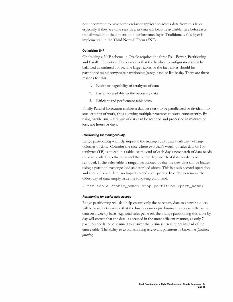
Partitioning for easier data access

Range partitioning will also help ensure only the necessary data to answer a query

will be scan. Lets assume that the business users predominately accesses the sales

data on a weekly basis, e.g. total sales per week then range partitioning this table by

day will ensure that the data is accessed in the most efficient manner, as only 7

partition needs to be scanned to answer the business users query instead of the

entire table. The ability to avoid scanning irrelevant partitions is known as partition

pruning.


S elect sum (sale s_am ount)

From SALES

W here sales_d ate betw een

to_date(‘05/20/2008’,’M M /D D/YYYY’)

A nd

to_date(‘05/23/2008’,’M M /D D/YYYY’);

Q : W hat w as the to tal sales for the

w eekend of M ay 20 - 22 2008?

O nly the 3 re levant partitions are acce sse d

Sales Tab le

M ay 22M ay 22n dn d 20082008

M ay 23M ay 23 rdrd 20 082008

M ay 24M ay 24 thth 20082 008

Ma y 18 t h 2008

M ay 19M ay 19 thth 20082 008

M ay 20M ay 20 thth 20082 008

M ay 21M ay 21stst 2 008200 8

Figure 7 Partition pruning: only the relevant partition is accessed

Partitioning for join performance

Sub-partitioning by hash is used predominately for performance reasons. Oracle

uses a linear hashing algorithm to create sub-partitions. In order to ensure that the

data gets evenly distributed among the hash partitions it is highly recommended

that the number of hash partitions is a power of 2 (for example, 2, 4, 8, etc). A

good rule of thumb to follow when deciding the number of hash partitions a table

should have is 2 X # of CPUs rounded to up to the nearest power of 2. If your

system has 12 CPUs then 32 would be a good number of hash partitions. On a

clustered system the same rules apply. If you have 3 nodes each with 4 CPUs then

32 would still be a good number of hash partitions. However, each hash partition

should be at least 16MB in size. Any small and they will not have efficient scan

rates with parallel query. If using the number of CPUs will make the size of the

hash partitions too small, use the number of RAC nodes in the environment

instead rounded to the nearest power of 2.

One of the main performance benefits of hash partitioning is partiton-wise joins.

Partition-wise joins reduce query response time by minimizing the amount of data

exchanged among parallel execution servers when joins execute in parallel. This

significantly reduces response time and improves both CPU and memory resource

usage. In a clustered data warehouse, this significantly reduces response times by

limiting the data traffic over the interconnect (IPC), which is the key to achieving

good scalability for massive join operations. Partition-wise joins can be full or

partial, depending on the partitioning scheme of the tables to be joined.

A full partition-wise join divides a join between two large tables into multiple

smaller joins. Each smaller join, performs a joins on a pair of partitions, one for

each of the tables being joined. For the optimizer to choose the full partition-wise

join method, both tables must be equi-partitioned on their join keys. That is, they

have to be partitioned on the same column with the same partitioning method.


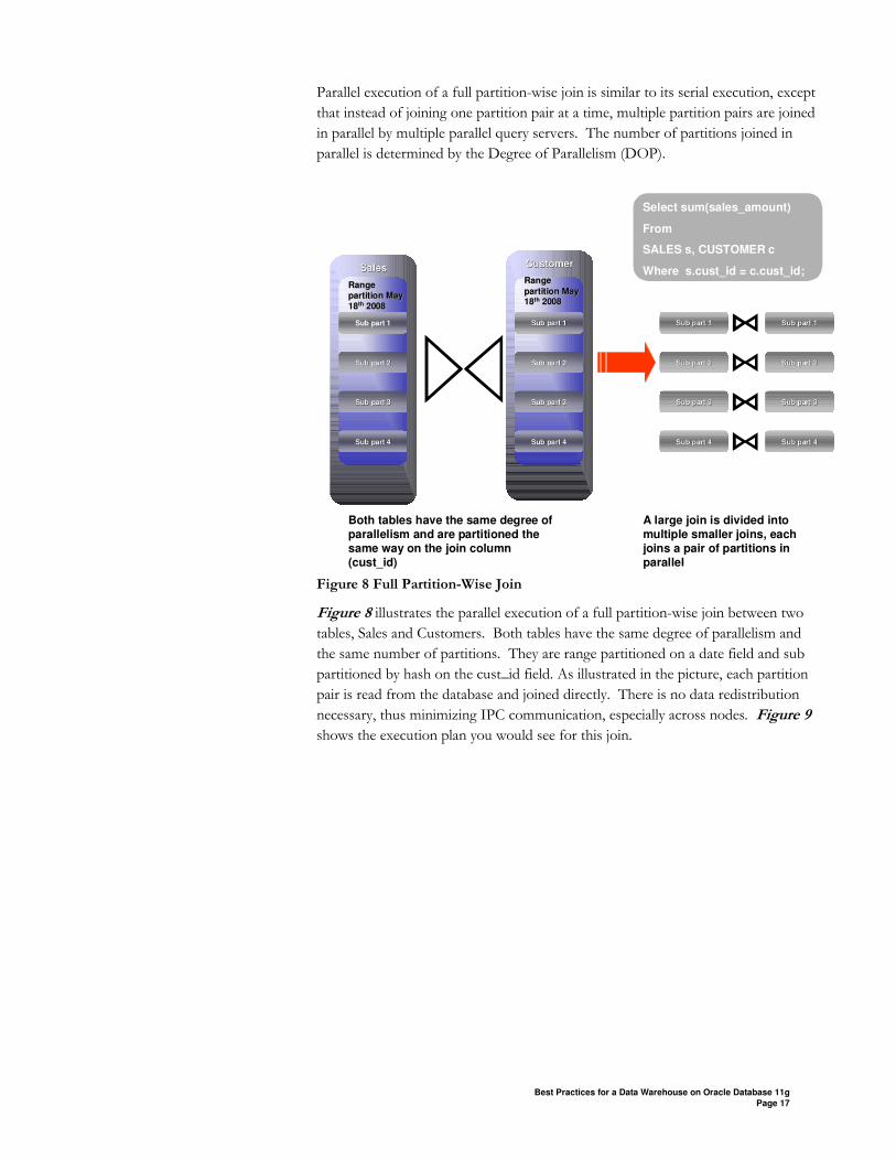
Parallel execution of a full partition-wise join is similar to its serial execution, except

that instead of joining one partition pair at a time, multiple partition pairs are joined

in parallel by multiple parallel query servers. The number of partitions joined in

parallel is determined by the Degree of Parallelism (DOP).

Select sum(sales_amount)

From

SALES s, CUSTOMER c

Where s.cust_id = c.cust_id;

Both tables have the same degree of parallelism and are partitioned the same way on the join column (cust_id)

SalesSales

Range Range

partition May partition May

1818thth 20082008

Sub part 2Sub part 2



Sub part 1

CustomerCustomer

Range Range

partition May partition May 1818thth 20082008













A large join is divided into multiple smaller joins, each joins a pair of partitions in parallel

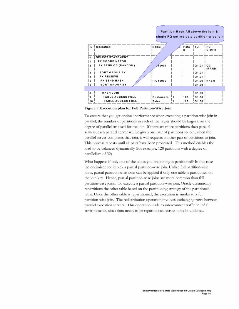
Figure 8 Full Partition-Wise Join

Figure 8 illustrates the parallel execution of a full partition-wise join between two

tables, Sales and Customers. Both tables have the same degree of parallelism and

the same number of partitions. They are range partitioned on a date field and sub

partitioned by hash on the cust_id field. As illustrated in the picture, each partition

pair is read from the database and joined directly. There is no data redistribution

necessary, thus minimizing IPC communication, especially across nodes. Figure 9

shows the execution plan you would see for this join.


H A S H

Q C

(R A N D )

P QD is tr ib

1 2 8

1 2 8

1 2 8

P stoP sto

pp

S E L E C T ST A T E M E N T0

Q 1,001S a lesT A B L E A C C E S S F U L L1 0

Q 1,001C u s to m e rsT A B L E A C C E S S F U L L9

Q 1,00H A S H JO IN 8

Q 1,001P X P A R T IT IO N H A S H A L L7

Q 1,00S O R T G R O U P B Y 6

Q 1,00:T Q 1 00 00P X S E N D H A S H 5

Q 1,01P X R E C E IV E 4

Q 1,01S O R T G R O U P B Y 3

Q 1,01:T Q 1 00 01P X S E N D Q C (R A N D O M )2

P X C O O R D IN A T O R 1

T QP sta rP sta r

ttN a m e N a m e O p e ra tio nO p e ra tio nIDID

P a rt it io n H as h A ll a b o ve th e jo in &

s in g le P Q s e t in d ic ate p a rt it io n -w is e jo in

Figure 9 Execution plan for Full Partition-Wise Join

To ensure that you get optimal performance when executing a partition-wise join in

parallel, the number of partitions in each of the tables should be larger than the

degree of parallelism used for the join. If there are more partitions than parallel

servers, each parallel server will be given one pair of partitions to join, when the

parallel server completes that join, it will requests another pair of partitions to join.

This process repeats until all pairs have been processed. This method enables the

load to be balanced dynamically (for example, 128 partitions with a degree of

parallelism of 32).

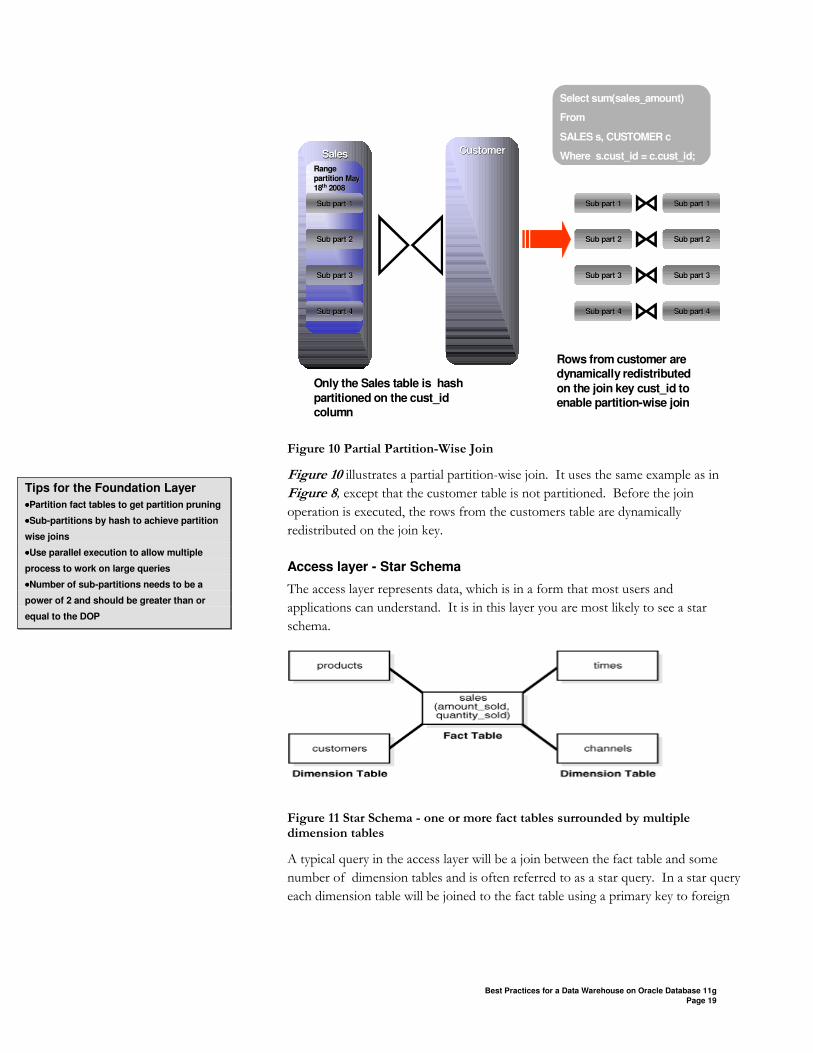
What happens if only one of the tables you are joining is partitioned? In this case

the optimizer could pick a partial partition-wise join. Unlike full partition-wise

joins, partial partition-wise joins can be applied if only one table is partitioned on

the join key. Hence, partial partition-wise joins are more common than full

partition-wise joins. To execute a partial partition-wise join, Oracle dynamically

repartitions the other table based on the partitioning strategy of the partitioned

table. Once the other table is repartitioned, the execution is similar to a full

partition-wise join. The redistribution operation involves exchanging rows between

parallel execution servers. This operation leads to interconnect traffic in RAC

environments, since data needs to be repartitioned across node boundaries.


Select sum(sales_amount)

From

SALES s, CUSTOMER c

Where s.cust_id = c.cust_id;

Only the Sales table is hash

partitioned on the cust_id

column

SalesSales

Range Range

partition May partition May

1818thth 20082008





CustomerCustomer









Rows from customer are

dynamically redistributed

on the join key cust_id to

enable partition-wise join

Figure 10 Partial Partition-Wise Join

Figure 10 illustrates a partial partition-wise join. It uses the same example as in

Figure 8, except that the customer table is not partitioned. Before the join

operation is executed, the rows from the customers table are dynamically

redistributed on the join key.

Access layer - Star Schema

The access layer represents data, which is in a form that most users and

applications can understand. It is in this layer you are most likely to see a star

schema.

Figure 11 Star Schema - one or more fact tables surrounded by multiple dimension tables

A typical query in the access layer will be a join between the fact table and some

number of dimension tables and is often referred to as a star query. In a star query

each dimension table will be joined to the fact table using a primary key to foreign

Tips for the Foundation Layer

••••Partition fact tables to get partition pruning

••••Sub-partitions by hash to achieve partition

wise joins

••••Use parallel execution to allow multiple

process to work on large queries

••••Number of sub-partitions needs to be a

power of 2 and should be greater than or

equal to the DOP


key join. Normally the dimension tables don’t join to each other. A business

question that could be asked against the star schema in Figure 11 would be “What

was the total number of umbrellas sold in Boston during the month of May 2008?”

The resulting SQL query for this question is shown in Figure 12.

Select SUM(s.quanity_sold) total, p.product, t.month

From Sales s, Customers c, Products p, Tim es t

W here s.cust_id = c.cust_id

And s.prod_id = p.prod_id

And s.time_id = t.time_id

And c.cust_city = ‘BOSTON’

And p.product = ‘UMBRELLA’

And t.month = ‘MAY’

And t.year = 2008;

Q: W hat was the total number of

umbrellas sold in Boston during

the month of May 2008 ?

Figure 12 Typical Star Query with all where clause predicates on the dimension

tables

As you can see all of the where clause predicates are on the dimension tables and

the fact table (Sales) is joined to each of the dimensions using their foreign key,

primary key relationship. So, how do you go about optimizing for this sytle of

query?

Optimizing Star Queries

Tuning a star query is very straight forward. The two most important criteria are;

• Create a bitmap index on each of the foreign key columns in the fact table or tables

• Set the initialization parameter STAR_TRANSFORMATION_ENABLED to TRUE. This will enable the optimizer feature for star queries which is off by default for backward compatibility.

If your environment meets these two criteria your star queries should use a

powerful optimization technique that will rewrite or transform you SQL called star

transformation. Star transformation executes the query in two phases, the first

phase retrieves the necessary rows from the fact table (row set) while the second

phase joins this row set to the dimension tables. The rows from the fact table are

retrieved by using bitmap joins between the bitmap indexes on all of the foreign key

columns. The end user never needs to know any of the details of

STAR_TRANSFORMATION, as the optimizer will automatically choose

STAR_TRANSFORMATION when its appropriate.


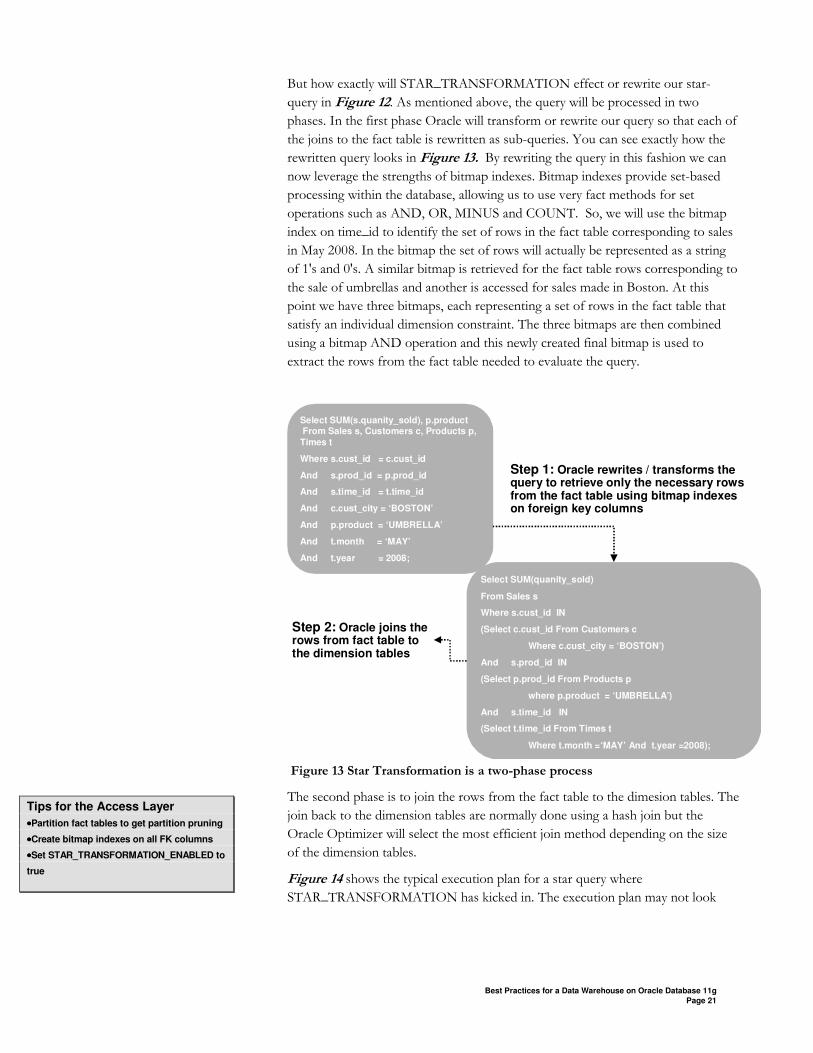
But how exactly will STAR_TRANSFORMATION effect or rewrite our star-

query in Figure 12. As mentioned above, the query will be processed in two

phases. In the first phase Oracle will transform or rewrite our query so that each of

the joins to the fact table is rewritten as sub-queries. You can see exactly how the

rewritten query looks in Figure 13. By rewriting the query in this fashion we can

now leverage the strengths of bitmap indexes. Bitmap indexes provide set-based

processing within the database, allowing us to use very fact methods for set

operations such as AND, OR, MINUS and COUNT. So, we will use the bitmap

index on time_id to identify the set of rows in the fact table corresponding to sales

in May 2008. In the bitmap the set of rows will actually be represented as a string

of 1's and 0's. A similar bitmap is retrieved for the fact table rows corresponding to

the sale of umbrellas and another is accessed for sales made in Boston. At this

point we have three bitmaps, each representing a set of rows in the fact table that

satisfy an individual dimension constraint. The three bitmaps are then combined

using a bitmap AND operation and this newly created final bitmap is used to

extract the rows from the fact table needed to evaluate the query.

Select SUM(s.quanity_sold), p.productFrom Sales s, Customers c, Products p,

Times t

Where s.cust_id = c.cust_id

And s.prod_id = p.prod_id

And s.time_id = t.time_id

And c.cust_city = ‘BOSTON’

And p.product = ‘UMBRELLA’

And t.month = ‘MAY’

And t.year = 2008;

Select SUM(quanity_sold)

From Sales s

Where s.cust_id IN

(Select c.cust_id From Customers c

Where c.cust_city = ‘BOSTON’)

And s.prod_id IN

(Select p.prod_id From Products p

where p.product = ‘UMBRELLA’)

And s.time_id IN

(Select t.time_id From Times t

Where t.month =‘MAY’ And t.year =2008);

Step 1: Oracle rewrites / transforms the query to retrieve only the necessary rows from the fact table using bitmap indexes on foreign key columns

Step 2: Oracle joins the rows from fact table to the dimension tables

Figure 13 Star Transformation is a two-phase process

The second phase is to join the rows from the fact table to the dimesion tables. The

join back to the dimension tables are normally done using a hash join but the

Oracle Optimizer will select the most efficient join method depending on the size

of the dimension tables.

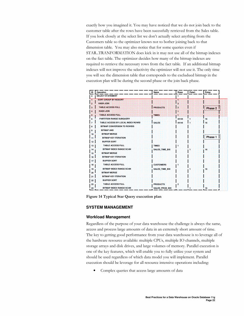
Figure 14 shows the typical execution plan for a star query where

STAR_TRANSFORMATION has kicked in. The execution plan may not look

Tips for the Access Layer

••••Partition fact tables to get partition pruning

••••Create bitmap indexes on all FK columns

••••Set STAR_TRANSFORMATION_ENABLED to

true


exactly how you imagined it. You may have noticed that we do not join back to the

customer table after the rows have been sucessfully retrieved from the Sales table.

If you look closely at the select list we don’t actually select anything from the

Customers table so the optimizer knows not to bother joining back to that

dimension table. You may also notice that for some queries even if

STAR_TRANFORMATION does kick in it may not use all of the bitmap indexes

on the fact table. The optimizer decides how many of the bitmap indexes are

required to retrieve the necessary rows from the fact table. If an additional bitmap

indexes will not improve the selectivity the optimizer will not use it. The only time

you will see the dimension table that corresponds to the excludued bitmap in the

execution plan will be during the second phase or the join back phase.

1

1

1

1

1

PstartPstart

BUFFER SORT22

2PRODUCTSTABLE ACCESS FULL23

1SELECT STATEMENT0

16SALES_PROD_BIXBITMAP INDEX RANGE SCAN24

BITMAP KEY ITERATION21

BITMAP MERGE20

16SALES_TIME_BIXBITMAP INDEX RANGE SCAN19

1CUSTOMERSTABLE ACCESS FULL18

BUFFER SORT17


BITMAP MERGE15

16SALES_TIME_BIXBITMAP INDEX RANGE SCAN14

1TIMESTABLE ACCESS FULL13

BUFFER SORT12


BITMAP MERGE10

BITMAP AND9

BITMAP CONVERSION TO ROWIDS8

1644144SALESTABLE ACCESS BY LOCAL INDEX ROWID 7

1644144PARTITION RANGE SUBQUERY6

1TIMESTABLE ACCESS FULL5

1HASH JOIN4

2PRODUCTSTABLE ACCESS FULL3

3HASH JOIN2

1SORT GROUP BY NOSORT 1

PstopPstopRowsRowsName Name OperationOperationIDID

Phase 2

Phase 1

Figure 14 Typical Star Query execution plan

SYSTEM MANAGEMENT

Workload Management

Regardless of the purpose of your data warehouse the challenge is always the same,

access and process large amounts of data in an extremely short amount of time.

The key to getting good performance from your data warehouse is to leverage all of

the hardware resource available: multiple CPUs, multiple IO channels, multiple

storage arrays and disk drives, and large volumes of memory. Parallel execution is

one of the key features, which will enable you to fully utilize your system and

should be used regardless of which data model you will implement. Parallel

execution should be leverage for all resource intensive operations including:

• Complex queries that access large amounts of data


• Building indexes on large tables

• Gathering Optimizer statistics

• Loading or manipulating large volumes of data

• Database backups

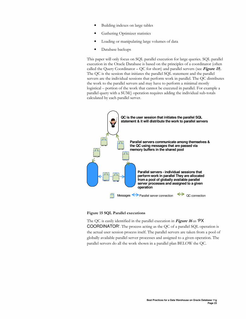
This paper will only focus on SQL parallel execution for large queries. SQL parallel execution in the Oracle Database is based on the principles of a coordinator (often called the Query Coordinator – QC for short) and parallel servers (see Figure 15). The QC is the session that initiates the parallel SQL statement and the parallel servers are the individual sessions that perform work in parallel. The QC distributes the work to the parallel servers and may have to perform a minimal mostly logistical – portion of the work that cannot be executed in parallel. For example a parallel query with a SUM() operation requires adding the individual sub-totals calculated by each parallel server.

MessagesMessages QC connectionParallel server connection

QC is the user session that initiates the parallel SQL statement & it will distribute the work to parallel servers

Parallel servers - individual sessions that perform work in parallel They are allocated from a pool of globally available parallel server processes and assigned to a given operation

Parallel servers communicate among themselves & the QC using messages that are passed via memory buffers in the shared pool

Figure 15 SQL Parallel executions

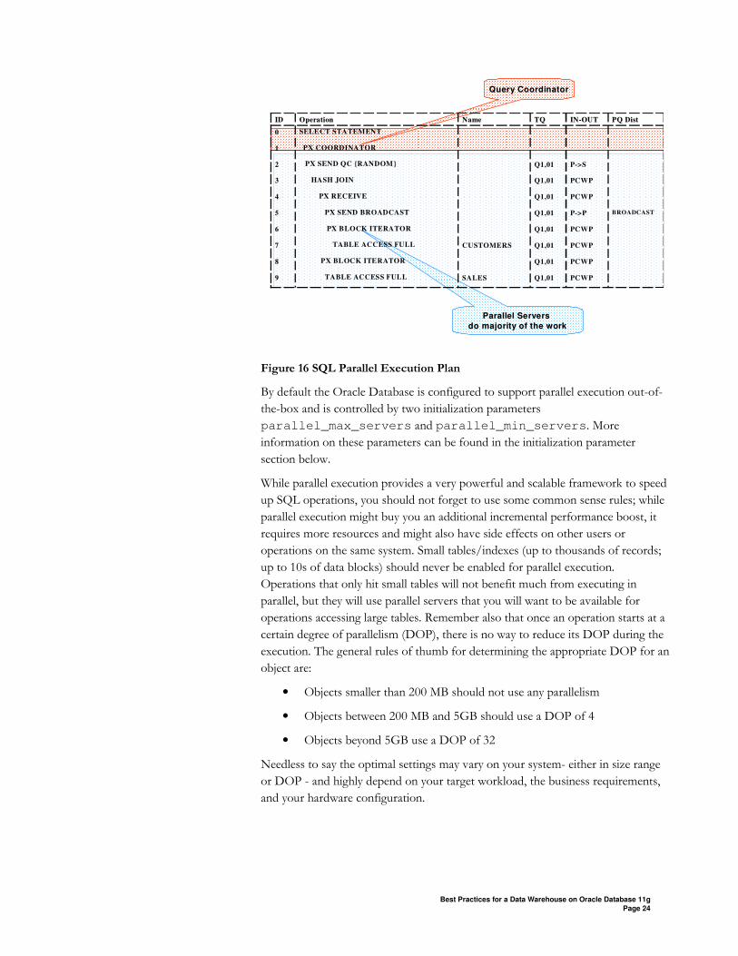
The QC is easily identified in the parallel execution in Figure 16 as 'PX

COORDINATOR'. The process acting as the QC of a parallel SQL operation is

the actual user session process itself. The parallel servers are taken from a pool of

globally available parallel server processes and assigned to a given operation. The

parallel servers do all the work shown in a parallel plan BELOW the QC.


Parallel Servers Parallel Servers

do majority of the workdo majority of the work

Query CoordinatorQuery Coordinator

BROADCASTP->PQ1,01PX SEND BROADCAST5

PCWP

PCWP

PCWP

PCWP

PCWP

PCWP

P->S

ININ--OUTOUT

SELECT STATEMENT0

Q1,01SALESTABLE ACCESS FULL 9

Q1,01PX BLOCK ITERATOR8

Q1,01CUSTOMERSTABLE ACCESS FULL 7

Q1,01PX BLOCK ITERATOR6

Q1,01PX RECEIVE4

Q1,01HASH JOIN3

Q1,01PX SEND QC {RANDOM}2

PX COORDINATOR 1

PQ DistPQ DistTQTQName Name OperationOperationIDID

Figure 16 SQL Parallel Execution Plan

By default the Oracle Database is configured to support parallel execution out-of-

the-box and is controlled by two initialization parameters

parallel_max_servers and parallel_min_servers. More

information on these parameters can be found in the initialization parameter

section below.

While parallel execution provides a very powerful and scalable framework to speed

up SQL operations, you should not forget to use some common sense rules; while

parallel execution might buy you an additional incremental performance boost, it

requires more resources and might also have side effects on other users or

operations on the same system. Small tables/indexes (up to thousands of records;

up to 10s of data blocks) should never be enabled for parallel execution.

Operations that only hit small tables will not benefit much from executing in

parallel, but they will use parallel servers that you will want to be available for

operations accessing large tables. Remember also that once an operation starts at a

certain degree of parallelism (DOP), there is no way to reduce its DOP during the

execution. The general rules of thumb for determining the appropriate DOP for an

object are:

• Objects smaller than 200 MB should not use any parallelism

• Objects between 200 MB and 5GB should use a DOP of 4

• Objects beyond 5GB use a DOP of 32

Needless to say the optimal settings may vary on your system- either in size range

or DOP - and highly depend on your target workload, the business requirements,

and your hardware configuration.


Whether or not to use cross instance parallel execution in RAC

By default the Oracle database enables inter-node parallel execution (parallel

execution of a single statement involving more than one node). As mentioned in

the balanced configuration section, the interconnect in a RAC environment must

be size appropriately as inter-node parallel execution may result in a lot of

interconnect traffic. If you are using a relatively weak interconnect in comparison to

the I/O bandwidth from the server to the storage subsystem, you may be better off

restricting parallel execution to a single node or to a limited number of nodes.

Inter-node parallel execution will not scale with an undersized interconnect. Use the

initialization parameters instance_groups and

parallel_instance_groups or database services to limit inter-node parallel

execution. It is recommended to use services beginning with Oracle database 11g.

Using Instance Groups to control Parallel Execution in RAC

The parameter instance_groups allows you to logically group different

instances together and perform inter-node parallel execution among all of the

associated instances. Instance groups can also be used to effectively partition

resources for a specific purpose, such as ETL, batch processing or ad-hoc querying.

Each active instance can be assigned to at least one or more instance groups. When

a particular instance group is activated, parallel operations will only spawn parallel

processes on instances in that group. Any instance group is made activity by setting

the parallel_instance_group parameter to one of the instance groups

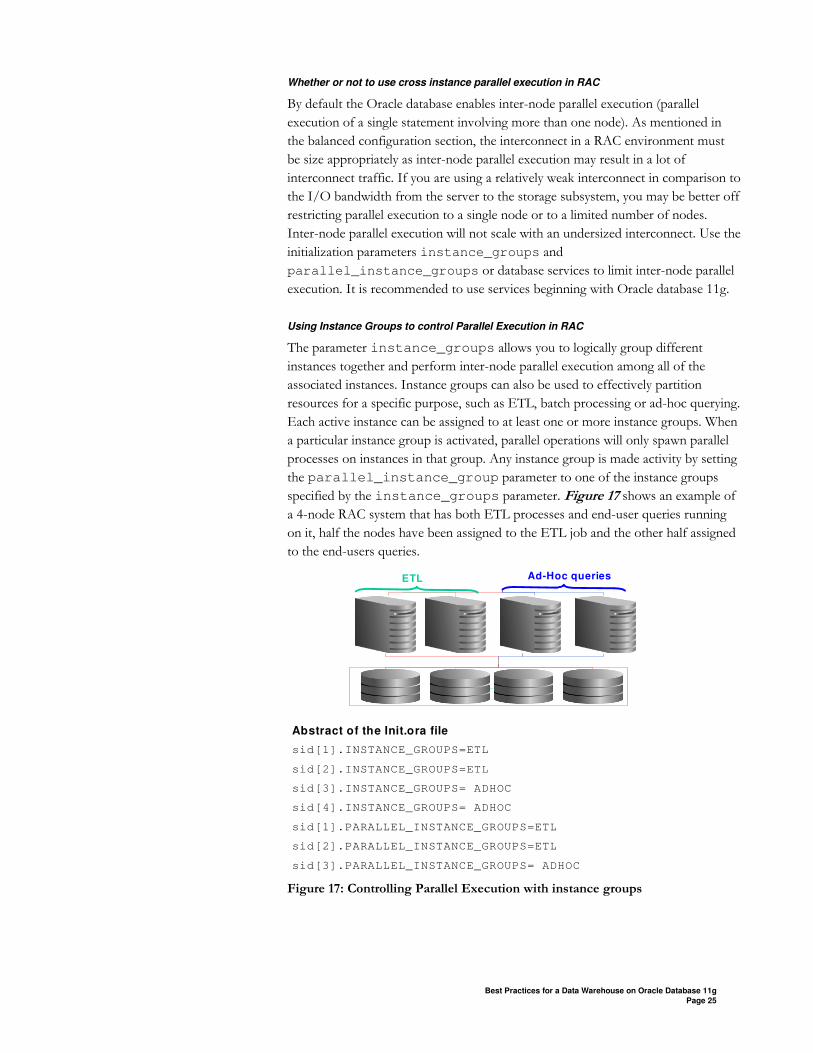
specified by the instance_groups parameter. Figure 17 shows an example of

a 4-node RAC system that has both ETL processes and end-user queries running

on it, half the nodes have been assigned to the ETL job and the other half assigned

to the end-users queries.

Abstract of the Init.ora file

sid[1].INSTANCE_GROUPS=ETL

sid[2].INSTANCE_GROUPS=ETL

sid[3].INSTANCE_GROUPS= ADHOC

sid[4].INSTANCE_GROUPS= ADHOC

sid[1].PARALLEL_INSTANCE_GROUPS=ETL

sid[2].PARALLEL_INSTANCE_GROUPS=ETL

sid[3].PARALLEL_INSTANCE_GROUPS= ADHOC

ETL Ad-Hoc queries

Figure 17: Controlling Parallel Execution with instance groups


Using services to control Parallel Execution in RAC

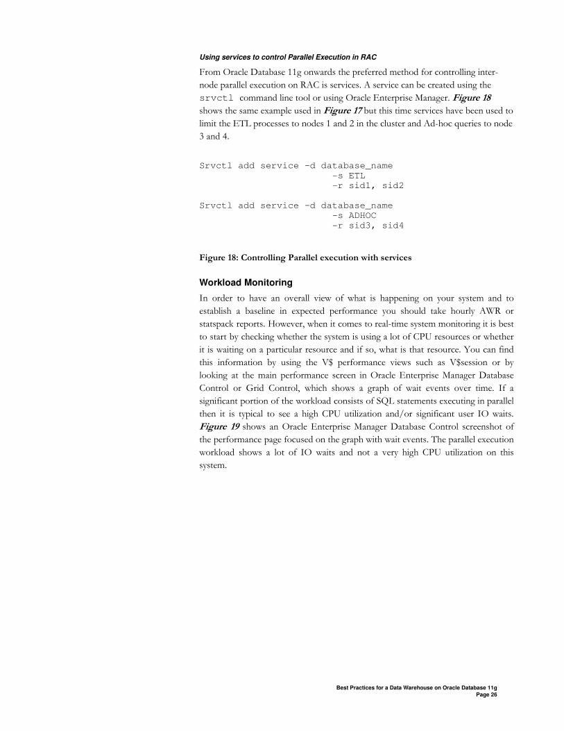
From Oracle Database 11g onwards the preferred method for controlling inter-

node parallel execution on RAC is services. A service can be created using the

srvctl command line tool or using Oracle Enterprise Manager. Figure 18

shows the same example used in Figure 17 but this time services have been used to

limit the ETL processes to nodes 1 and 2 in the cluster and Ad-hoc queries to node

3 and 4.

Srvctl add service –d database_name

-s ETL

-r sid1, sid2

Srvctl add service –d database_name

-s ADHOC

-r sid3, sid4

Figure 18: Controlling Parallel execution with services

Workload Monitoring

In order to have an overall view of what is happening on your system and to

establish a baseline in expected performance you should take hourly AWR or

statspack reports. However, when it comes to real-time system monitoring it is best

to start by checking whether the system is using a lot of CPU resources or whether

it is waiting on a particular resource and if so, what is that resource. You can find

this information by using the V$ performance views such as V$session or by

looking at the main performance screen in Oracle Enterprise Manager Database

Control or Grid Control, which shows a graph of wait events over time. If a

significant portion of the workload consists of SQL statements executing in parallel

then it is typical to see a high CPU utilization and/or significant user IO waits.

Figure 19 shows an Oracle Enterprise Manager Database Control screenshot of

the performance page focused on the graph with wait events. The parallel execution

workload shows a lot of IO waits and not a very high CPU utilization on this

system.


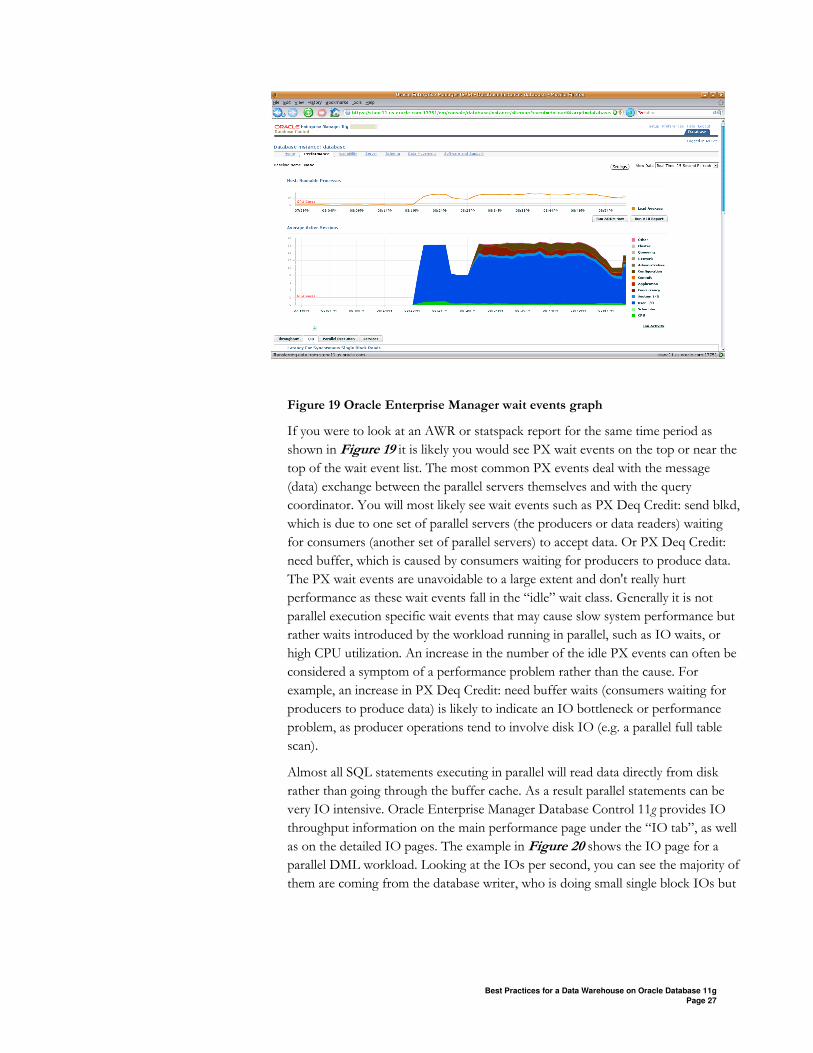
Figure 19 Oracle Enterprise Manager wait events graph

If you were to look at an AWR or statspack report for the same time period as

shown in Figure 19 it is likely you would see PX wait events on the top or near the

top of the wait event list. The most common PX events deal with the message

(data) exchange between the parallel servers themselves and with the query

coordinator. You will most likely see wait events such as PX Deq Credit: send blkd,

which is due to one set of parallel servers (the producers or data readers) waiting

for consumers (another set of parallel servers) to accept data. Or PX Deq Credit:

need buffer, which is caused by consumers waiting for producers to produce data.

The PX wait events are unavoidable to a large extent and don't really hurt

performance as these wait events fall in the “idle” wait class. Generally it is not

parallel execution specific wait events that may cause slow system performance but

rather waits introduced by the workload running in parallel, such as IO waits, or

high CPU utilization. An increase in the number of the idle PX events can often be

considered a symptom of a performance problem rather than the cause. For

example, an increase in PX Deq Credit: need buffer waits (consumers waiting for

producers to produce data) is likely to indicate an IO bottleneck or performance

problem, as producer operations tend to involve disk IO (e.g. a parallel full table

scan).

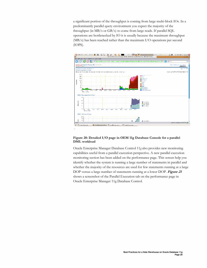
Almost all SQL statements executing in parallel will read data directly from disk

rather than going through the buffer cache. As a result parallel statements can be

very IO intensive. Oracle Enterprise Manager Database Control 11g provides IO

throughput information on the main performance page under the “IO tab”, as well

as on the detailed IO pages. The example in Figure 20 shows the IO page for a

parallel DML workload. Looking at the IOs per second, you can see the majority of

them are coming from the database writer, who is doing small single block IOs but


a significant portion of the throughput is coming from large multi-block IOs. In a

predominantly parallel query environment you expect the majority of the

throughput (in MB/s or GB/s) to come from large reads. If parallel SQL

operations are bottlenecked by IO it is usually because the maximum throughput

(MB/s) has been reached rather than the maximum I/O operations per second

(IOPS).

Figure 20: Detailed I/O page in OEM 11g Database Console for a parallel DML workload

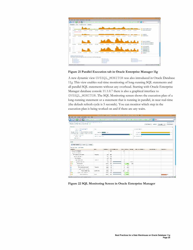
Oracle Enterprise Manager Database Control 11g also provides new monitoring

capabilities useful from a parallel execution perspective. A new parallel execution

monitoring section has been added on the performance page. This screen help you

identify whether the system is running a large number of statements in parallel and

whether the majority of the resources are used for few statements running at a large

DOP versus a large number of statements running at a lower DOP. Figure 21

shows a screenshot of the Parallel Execution tab on the performance page in

Oracle Enterprise Manager 11g Database Control.

.


Figure 21 Parallel Execution tab in Oracle Enterprise Manager 11g

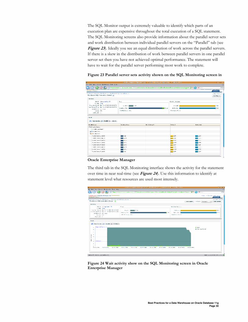
A new dynamic view GV$SQL_MONITOR was also introduced in Oracle Database

11g. This view enables real-time monitoring of long-running SQL statements and

all parallel SQL statements without any overhead. Starting with Oracle Enterprise

Manager database console 11.1.0.7 there is also a graphical interface to

GV$SQL_MONITOR. The SQL Monitoring screen shows the execution plan of a

long-running statement or a statement that is running in parallel, in near real-time

(the default refresh cycle is 5 seconds). You can monitor which step in the

execution plan is being worked on and if there are any waits.

Figure 22 SQL Monitoring Screen in Oracle Enterprise Manager


The SQL Monitor output is extremely valuable to identify which parts of an

execution plan are expensive throughout the total execution of a SQL statement.

The SQL Monitoring screens also provide information about the parallel server sets

and work distribution between individual parallel servers on the “Parallel” tab (see

Figure 23). Ideally you see an equal distribution of work across the parallel servers.

If there is a skew in the distribution of work between parallel servers in one parallel

server set then you have not achieved optimal performance. The statement will

have to wait for the parallel server performing most work to complete.

Figure 23 Parallel server sets activity shown on the SQL Monitoring screen in

Oracle Enterprise Manager

The third tab in the SQL Monitoring interface shows the activity for the statement

over time in near real-time (see Figure 24). Use this information to identify at

statement level what resources are used most intensely.

Figure 24 Wait activity show on the SQL Monitoring screen in Oracle Enterprise Manager


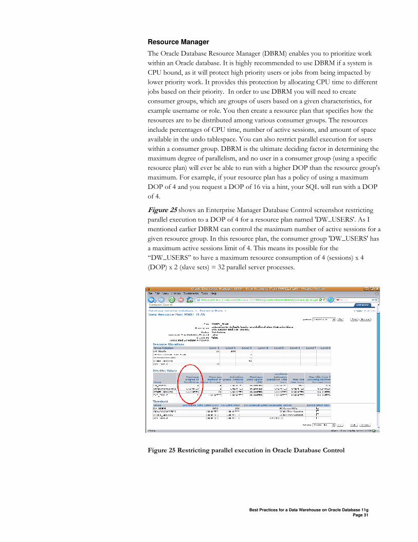
Resource Manager

The Oracle Database Resource Manager (DBRM) enables you to prioritize work

within an Oracle database. It is highly recommended to use DBRM if a system is

CPU bound, as it will protect high priority users or jobs from being impacted by

lower priority work. It provides this protection by allocating CPU time to different

jobs based on their priority. In order to use DBRM you will need to create

consumer groups, which are groups of users based on a given characteristics, for

example username or role. You then create a resource plan that specifies how the

resources are to be distributed among various consumer groups. The resources

include percentages of CPU time, number of active sessions, and amount of space

available in the undo tablespace. You can also restrict parallel execution for users

within a consumer group. DBRM is the ultimate deciding factor in determining the

maximum degree of parallelism, and no user in a consumer group (using a specific

resource plan) will ever be able to run with a higher DOP than the resource group's

maximum. For example, if your resource plan has a policy of using a maximum

DOP of 4 and you request a DOP of 16 via a hint, your SQL will run with a DOP

of 4.

Figure 25 shows an Enterprise Manager Database Control screenshot restricting

parallel execution to a DOP of 4 for a resource plan named 'DW_USERS'. As I

mentioned earlier DBRM can control the maximum number of active sessions for a

given resource group. In this resource plan, the consumer group 'DW_USERS' has

a maximum active sessions limit of 4. This means its possible for the

“DW_USERS” to have a maximum resource consumption of 4 (sessions) x 4

(DOP) x 2 (slave sets) = 32 parallel server processes.

Figure 25 Restricting parallel execution in Oracle Database Control


Optimizer Statistics Management

Knowing when and how to gather optimizer statistics has become somewhat of

dark art especially in a data warehouse environment where statistics maintenance

can be hindered by the fact that as the data set increases the time it takes to gather

statistics will also increase. By default the DBMS_STATS packages will gather

global (table level), partition level, and sub-partition statistics for each of the tables

in the database. The only exception to this is if you have hash sub-partitions. Hash

sub-partitions do not need statistics, as the optimizer can accurately derive any

necessary statistics from the partition level statistic because the hash partitions are

all approximately the same size due to linear hashing algorithm.

As mentioned above the length of time it takes to gather statistics will grow

proportionally with your data set, so you may now be wondering if the optimizer

truly need statistics at every level for a partitioned table or if time could be saved by

skipping one or more levels? The short answer is “no” as the optimizer will use

statistics from one or more of the levels in different situations.

• The optimizer will use global or table level statistics if one or more of your

queries touches two or more partitions.

• The optimizer will use partition level statistics if your queries do partition

elimination, such that only one partition is necessary to answer each query.

If your queries touch two or more partitions the optimizer will use a

combination of global and partition level statistics.

• The optimizer will user sub-partition level statistics if your queries do

partition elimination, such that only one sub-partition is necessary. If your

queries touch two more sub-partitions the optimizer will use a

combination of sub-partition and partition level statistics.

Global statistics are by far the most important statistics but they also take the

longest time to collect because a full table scan is required. However, in Oracle

Database 11g this issue has been addressed with the introduction of Incremental

Global statistics. Typically with partitioned tables, new partitions are added and

data is loaded into these new partitions. After the partition is fully loaded, partition

level statistics need to be gathered and the global statistics need to be updated to

reflect the new data. If the INCREMENTAL value for the partition table is set to

TRUE, and the DBMS_STATS GRANULARITY parameter is set to AUTO, Oracle

will gather statistics on the new partition and update the global table statistics by

scanning only those partitions that have been modified and not the entire table.

Below are the steps necessary to do use incremental global statistics

SQL> exec dbms_stats.set_table_prefs('SH', 'SALES',

'INCREMENTAL', 'TRUE');

SQL> exec dbms_stats.gather_table_stats( Owner=>'SH', Tabname=>'SALES', Partname=>’23_MAY_2008’, Granularity=>’AUTO’);


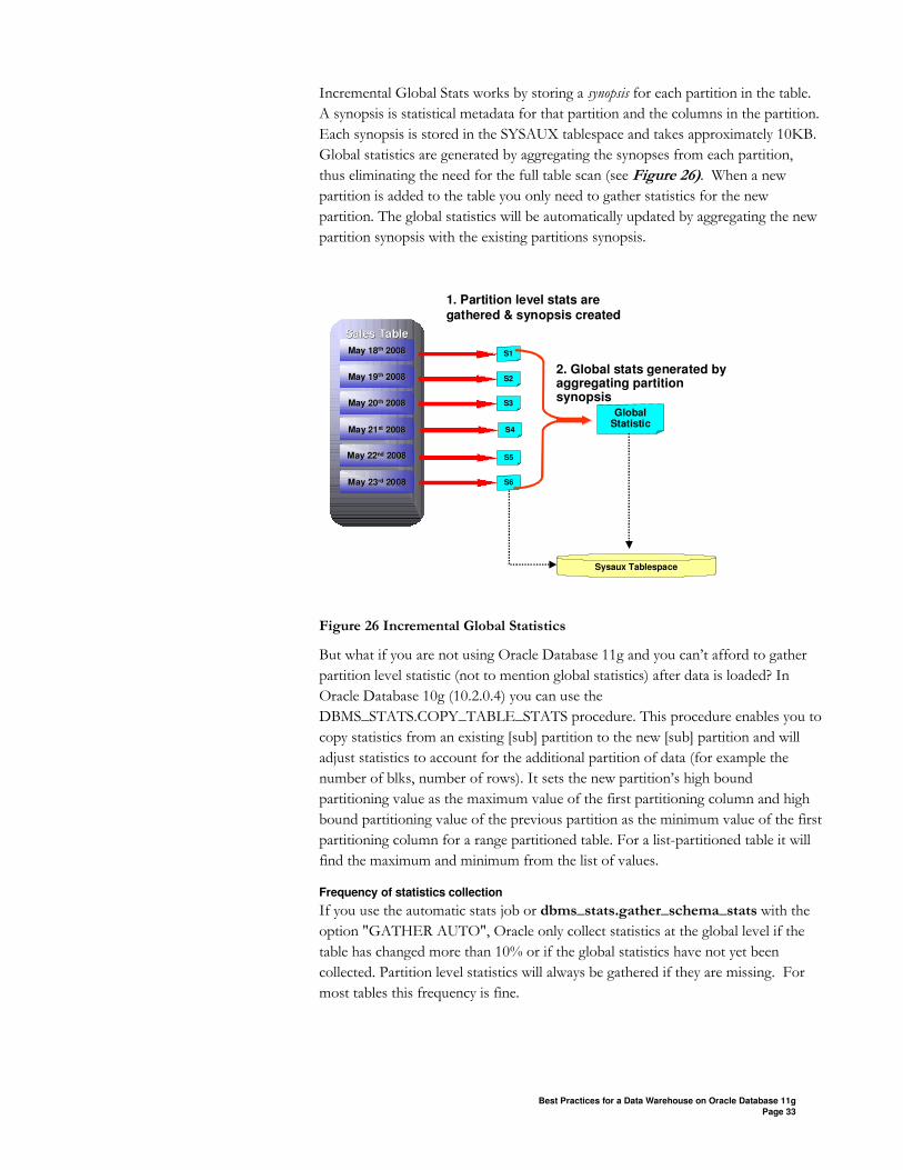
Incremental Global Stats works by storing a synopsis for each partition in the table.

A synopsis is statistical metadata for that partition and the columns in the partition.

Each synopsis is stored in the SYSAUX tablespace and takes approximately 10KB.

Global statistics are generated by aggregating the synopses from each partition,

thus eliminating the need for the full table scan (see Figure 26). When a new

partition is added to the table you only need to gather statistics for the new

partition. The global statistics will be automatically updated by aggregating the new

partition synopsis with the existing partitions synopsis.

Sales TableSales Table

May 22May 22ndnd 20082008

May 23May 23rdrd 20082008

May 18May 18thth 20082008



May 21May 21stst 20082008

Sysaux Tablespace

S1

S2

S3

S4

S5

S6

1. Partition level stats are gathered & synopsis created

Global Statistic

2. Global stats generated by aggregating partition synopsis

Figure 26 Incremental Global Statistics

But what if you are not using Oracle Database 11g and you can’t afford to gather

partition level statistic (not to mention global statistics) after data is loaded? In

Oracle Database 10g (10.2.0.4) you can use the

DBMS_STATS.COPY_TABLE_STATS procedure. This procedure enables you to

copy statistics from an existing [sub] partition to the new [sub] partition and will

adjust statistics to account for the additional partition of data (for example the

number of blks, number of rows). It sets the new partition’s high bound

partitioning value as the maximum value of the first partitioning column and high

bound partitioning value of the previous partition as the minimum value of the first

partitioning column for a range partitioned table. For a list-partitioned table it will

find the maximum and minimum from the list of values.

Frequency of statistics collection

If you use the automatic stats job or dbms_stats.gather_schema_stats with the

option "GATHER AUTO", Oracle only collect statistics at the global level if the

table has changed more than 10% or if the global statistics have not yet been

collected. Partition level statistics will always be gathered if they are missing. For

most tables this frequency is fine.


However, in a data warehouse environment there is one scenario where this is not

the case. If a partition table is constantly having new partitions added and then data

is loaded into the new partition and users instantly begin querying the new data,

then it is possible to get a situation where an end-users query will supply a value in

one of the where clause predicate that is outside the [min,max] range for the

column according to the optimizer statistics. For predicate values outside the

statistics [min,max] range the optimizer will prorates the selectivity for that

predicate based on the distance between the value the max (assuming the value is

higher than the max). This means, the farther the value is from the maximum value

the lower is the selectivity will be, which may result in sub-optimal execution plans.

You can avoid this “Out of Range” situation by using the new incremental global

statistics or the copy table statistics procedure.

Initialization Parameter

There are a few parameters that you should pay close attention to when it comes to

achieving good performance on a data warehouse environment. However, it is

strongly recommend that you leave the majority of the initialization parameter at

their default values.

Memory allocation

Large parallel operations may use a lot of execution memory, and you should take

this into account when allocating memory to the database. You should also bear in

mind that the majority of operations that execute in parallel bypass the buffer

cache. A parallel operation will only use the buffer cache if the object has been

explicitly created with the cache option or if the object size is smaller than 2% of

the buffer cache. If the object size is less than 2% of the buffer cache then the cost

of the checkpoint to start the direct read is deemed more expensive than just

reading the blocks into the cache.

shared_pool_size Parallel servers communicate among themselves and with

the Query Coordinator by passing messages. The messages are passed via memory

buffers that are allocated from the shared pool. When a parallel server is started it

will allocate buffers in the shared pool so it can communicate, if there is not

enough free space in the shared pool to allocate the buffers the parallel server will

fail to start. In order to size your shared pool appropriately you should use the

following formulas to calculate the additional overhead parallel servers will put on

the shared pool. If you are running on a single SMP machine or you are doing

inter-node parallel operations

Memory = #Of Users * DOP * (4 + 2 * DOP)*parallel_execution_message_size

The expression (4+2*DOP) in the equation comes from the number of buffers

needed for the parallel servers to communicate during a SQL execution. Typically

there will be two sets of parallel servers (a producer and a consumer) per query.

The number of parallel servers in each set will be equal to the DOP. Each parallel

server needs 2 buffers to communicate with the query coordinator (2 for each


producer + 2 for each consumer =4). While each parallel server pair (1 producer

and 1 consumer) will share a pair of buffers so they can communicate (2*DOP).

If you are using cross instance parallel operation in a RAC environment

Memory per instance = Users * (DOP / NumberOfInstances * (2 + 2 *

DOP/NumberOfInstances + 4 * (DOP – DOP/NumberOfInstances)) *

parallel_execution_message_size

When running cross instance parallel operations in a RAC environment the parallel

slaves will be spawned across all of the nodes. That is why you see the

DOP/NumberOfInstances in this equation, as it calculates the additional memory

required per instance or node.

The expression (DOP / NumberOfInstances * (2 + 2 *

DOP/NumberOfInstances + 4 * (DOP – DOP/NumberOfInstances)) again

represents the number of communication buffers needed. As with the previous

case each parallel slave on the local node needs 2 buffers to communicate with the

query coordinator. And each local parallel slave pair (one producer, one consumer)

will share a pair of buffers so they can communicate (2*DOP), thus

2+2*DOP/NumberOfInstances.

Each local parallel server must also communicate with each remote parallel server.

For each local parallel server two additional message buffers are required for each

remote parallel server (2 for the producer + 2 for the consumer=4). The number of

remote parallel servers is calculated by subtracting the number of local parallel

servers from the total number of parallel servers or the DOP (DOP –

DOP/NumberOfInstances). Thus giving 4 * (DOP – DOP/NumberOfInstances).

Note the results of both these equations are returned in bytes.

Only the memory needed for the parallel_min_servers will be pre-allocated

from the shared_pool at database startup. As additional parallel servers are needed,

their memory buffers will be allocated “on the fly” from the shared pool. These

rules apply irrespective of whether you use shared_pool_size directly, or

sga_target (10g and higher) or memory_target (starting with 11g).

pga_aggregate_target: The pga_aggregate_target parameter

controls the total amount of execution memory that can be allocated by Oracle.

Oracle attempts to keep the amount of private memory below the target you

specified by adapting the size of the work areas. When you increase the value of

this parameter, you indirectly increase the memory allotted to work areas.

Consequently, more memory-intensive operations are able to run fully in memory

and not spill over to disk. For environments that run a lot of parallel operations

you should set pga_aggregate_target as large as possible. A good rule of

thumb is to have a minimum of 100MB X parallel_max_servers.


Controlling Parallel Execution

parallel_execution_message_size: As mentioned above, the Parallel

servers communicate among themselves and with the Query Coordinator by

passing messages via memory buffers. If you execute a lot of large operations in

parallel, it’s advisable to reduce the messaging latency by increasing the

parallel_execution_message_size (the size of the buffers). By default

the message size is 2K. Ideally you should increase it to 16k (16384). However, a

larger parallel_execution_message_size will increase the memory

requirement for the shared_pool so if you increase it from 2K to 16K your parallel

server memory requirement will be 8 X more.

In order for a parallel operation to execute in an optimal fashion there has to be

enough parallel servers available. If there are no parallel servers available the

operation will actually be executed serially.

parallel_min_servers: This parameter determines the number of parallel

servers that will be started during database startup. By default the value is 0. It is

recommended that you set parallel_min_servers to

Average # of concurrent queries * maximum DOP needed by a query

This will ensure that there are ample parallel server processes available for the

majority of the queries executed on the system and queries will not suffer any

additional overhead of having to spawn extra parallel servers. However, if extra

parallel servers are required for additional queries above you average workload they

can be spawned “on the fly” up to the value of parallel_max_servers.

Bear in mind that any additional parallel server processes that are spawned above

parallel_min_servers will be killed after they have been inactive for a

certain about of time and will have to be re-spawned if they are need again in the

future.

parallel_max_servers: This parameter determines the maximum number of

parallel servers that may be started for a database instance, should there be demand

for them. The default value for Oracle Database 10g and higher is 10 *

cpu_count * parallel_threads_per_cpu. A good rule of thumb is to

ensure parallel_max_servers is set to a number greater than

Maximum # of concurrent queries * maximum DOP needed by a query

By doing this you will ensure every query gets the appropriate number of parallel

servers.

parallel_adaptive_multi_user For predictable response times on a busy

server it is better to set this parameter to false.

Enabling efficient IO throughput

db_block_size should be 8K,16K or 32K. Larger block sizes help to facilitate

data compression as Oracle does its compression at the database block level by

eliminating duplicate values within a block.


db_file_multiblock_read_count SQL parallel execution is generally used

for queries that will access a lot of data, for example when doing a full table scan.

Since parallel execution will by-pass the buffer cache and access data directly from

disk you want each I/O to be as efficient as possible, and using large I/Os is a way

to reduce latency.

Set db_file_multiblock_read_count to 1024/db_block_size. E.g. for 8K

block size, use db_file_multiblock_read_count=128.

disk_async_io For optimum performance make sure you use asynchronous

I/Os. This is the default value for the majority of platforms.

Star Query

Star_transformation_enabled controls whether or not the optimizer will use a cost-

based transformation on queries in a star schema. By default this parameter is set

too false. If you have a star schema and you have created a bitmap index on the

foreign key columns of the fact table you should set this parameter to true.

CONCLUSION

In order to guarantee you will get the optimal performance from your data

warehouse and to ensure it will scale as the data set increases you need to get three

fundamental things correct:

• The hardware configuration. It must be balanced and must achieve the

necessary IO throughput required to meet the systems peak load.,

• The data model. If it is a 3NF it should always achieve partition-wise joins

or if it’s a Star Schema it should use star transformation,

• The data loading process. It should be as fast as possible and have zero

impact on the business user.

By designing these three corner stones correctly you can seamlessly scale out your

EDW without having to constantly tune or tweak the system.

Tips for System Management

••••Use Parallel Execution where appropriate

••••Take hourly AWR or statspack report

••••Use EM to do real-time system monitoring

••••Use Resource Manager to ensure necessary

users get high priority on the system

••••Always have accurate Optimizer statistics

••••Use INCREMENTAL statistic maintenance or

copy_stats to keep large partitioned fact -

table up to date in a timely manner

••••Set only the initialization parameters that

you need to

Data Warehouse Best Practices for Oracle Database 11g

September 2008

Author: Maria Colgan

Contributing Authors: Doug Cackett, George Spears, and Andrew Bond

Oracle Corporation

World Headquarters

500 Oracle Parkway

Redwood Shores, CA 94065

U.S.A.

Worldwide Inquiries:

Phone: +1.650.506.7000

Fax: +1.650.506.7200

oracle.com

Copyright © 2008, Oracle. All rights reserved.

This document is provided for information purposes only and the

contents hereof are subject to change without notice.

This document is not warranted to be error-free, nor subject to any

other warranties or conditions, whether expressed orally or implied

in law, including implied warranties and conditions of merchantability

or fitness for a particular purpose. We specifically disclaim any

liability with respect to this document and no contractual obligations

are formed either directly or indirectly by this document. This document

may not be reproduced or transmitted in any form or by any means,

electronic or mechanical, for any purpose, without our prior written permission.

Oracle is a registered trademark of Oracle Corporation and/or its affiliates.

Other names may be trademarks of their respective owners.

best practices for a data warehouse on oracle database … · best practices for a data warehouse...

Documents