bel ventutorial hetero
TRANSCRIPT
An Introduction toRobust Estimation with
R Functions
Ruggero BellioDepartment of Statistics, University of Udine
Laura VenturaDepartment of Statistics, University of Padova
October 2005
Contents
1 Introduction 2
2 Estimation in scale and location models 72.1 The function mean for a trimmed mean . . . . . . . . . . . . . . . . . . . . 82.2 The functions median and mad . . . . . . . . . . . . . . . . . . . . . . . . . 102.3 The huber and hubers functions . . . . . . . . . . . . . . . . . . . . . . . 122.4 An introduction to the rlm function . . . . . . . . . . . . . . . . . . . . . . 14
3 Estimation in scale and regression models 173.1 M-estimators . . . . . . . . . . . . . . . . . . . . . . . . . . . . . . . . . . 183.2 The weighted likelihood . . . . . . . . . . . . . . . . . . . . . . . . . . . . 263.3 High breakdown regression . . . . . . . . . . . . . . . . . . . . . . . . . . . 293.4 Bounded-influence estimation in linear regression models . . . . . . . . . . 32
4 Bounded-influence estimation in logistic regression 444.1 Mallows-type estimation . . . . . . . . . . . . . . . . . . . . . . . . . . . . 454.2 The Bianco and Yohai estimator . . . . . . . . . . . . . . . . . . . . . . . . 46

1 Introduction
Since 1960, many theoretical e!orts have been devoted to develop statistical proceduresthat are resistant to small deviations from the assumptions, i.e. robust with respect tooutliers and stable with respect to small deviations from the assumed parametric model.In fact, it is well-known that classical optimum procedures behave quite poorly underslight violations of the strict model assumptions.
It is also well-known that to screen the data, to remove outliers and then to applyclassical inferential procedures is not a simple and good way to proceed. First of all, inmultivariate or highly structured data, it can be di"cult to single out outliers or it canbe even impossible to identify influential observations. Second, in place of rejecting anobservation, it could be better to down-weight uncertain observations, although we maywish to reject completely wrong observations. Moreover, rejecting outliers reduces thesample size, could a!ect the distribution theory, and variances could be underestimatedfrom the cleaned data. Finally, empirical evidence shows that good robust proceduresbehave quite better than techniques based on the rejection of outliers.
Robust statistical procedures focus in estimation, testing hypotheses and in regressionmodels. There exist a great variety of approaches toward the robustness problem. Amongthese, procedures based on M-estimators (and gross error sensitivity) and high breakdownpoint estimators (and breakdown point) play an important and complementary role. Thebreakdown point of an estimator is the largest fraction of the data that can be movedarbitrarily without perturbing the estimator to the boundary of the parameter space:thus the higher the breakdown point, the more robust the estimator against extremeoutliers. However, the breakdown point is not enough to assess the degree of robustnessof an estimator. Instead, the gross error sensitivity gives an exact measure of the size ofrobustness, since it is the supremum of the influence function of an estimator, and it isa measure of the maximum e!ect an observation can have on an estimator. There aresome books on robust statistics. Huber (1981) and Hampel et al. (1986) are the maintheoretical ones; see also Staudte and Sheather (1990). Rousseeuw and Leroy (1987) ismore practical.
At present, the practical application of robust methods is still limited and the proposalsconcern mainly a specific class of applications (typically estimation of scale and regressionmodels, which include location and scale models). In view of this, a considerable amountof new programming in R is requested. Two books about practical application of robustmethods with S and R functions are Marazzi (1993) and Venables and Ripley (2002).
An example: Chushny and Peebles data
The data plotted in Figure 1 concern n = 10 observations on the prolongation of sleep bymeans of two drugs (see Chushny and Peebles, 1905, and Hampel et al., 1986, chap. 2).These data have been used by Student as the first illustration of a t-test, to investigatewhether a significant di!erence existed between the observed e!ect of both drugs.
> xdat <- c(0.0,0.8,1.0,1.2,1.3,1.3,1.4,1.8,2.4,4.6)> boxplot(xdat)
The boxplot is a useful plot since it allows to identify possible outliers and to look at theoverall shape of a set of observed data, particularly for large data sets.
2

01
23
4
Figure 1: Chushny and Peebles data.
Most authors have considered these data as a normally distributed sample and forinferential purposes have applied the usual t-test. For instance, to test for a null mean orto give a confidence interval for the mean, the function t.test can be used.
> t.test(xdat)
One Sample t-test
data: xdatt = 4.0621, df = 9, p-value = 0.002833alternative hypothesis: true mean is not equal to 095 percent confidence interval:0.7001142 2.4598858sample estimates:mean of x
1.58> mean(xdat)[1] 1.58> sd(xdat)[1] 1.229995> t.test(xdat)$conf.int[1] 0.7001142 2.4598858attr(,"conf.level")[1] 0.95
However, the boxplot in Figure 1 reveals that the normality assumption could be ques-tionable, and the value 4.6 appears to be an outlier. An outlier is a sample value thatcause surprise in relation to the majority of the sample. If this value is not considered inthe analysis, the value of the arithmetic mean changes (the mean is shifted in the positivedirection of the outlier), but the relevant e!ect is mainly on the classical estimate of thescale parameter (see, for example, the 95 percent confidence interval).
> t.test(xdat[1:9])$statistict
5.658659> t.test(xdat[1:9])$p.value
3

[1] 0.0004766165> mean(xdat[1:9])[1] 1.244444> sd(xdat[1:9])[1] 0.6597558> t.test(xdat[1:9])$conf.int[1] 0.7373112 1.7515777attr(,"conf.level")[1] 0.95
In this situation, the value 4.6 is considered as an outlier for the Gaussian model, butthere is no so much information (only n = 10 observations) to assume a longer taileddistribution for the data. In this case, robust methods for estimation of the scale andlocation parameters could be useful.
An example: Regression model
Suppose that the points in Figure 2 represent the association between vacation expensesand wealth of n = 13 fictitious individuals (see Marazzi, 1993). Three di!erent models areconsidered: the first one (fit1) is based on all the observations, the second one (fit2)considers also a quadratic term in x in the linear predictor, and the last one (fit3) iswithout the leverage observation.
> xx <- c(0.7,1.1,1.2,1.7,2,2.1,2.1,2.5,1.6,3,3.2,3.5,8.5)> yy <- c(0.5,0.6,1,1.6,0.9,1.6,1.5,2,2.1,2.5,2.2,3,0.5)> plot(xx,yy,xlim=c(0,10),ylim=c(0,6))> fit1 <- lm(yy~xx)> abline(fit1$coef,lty=1)> fit2 <- lm(yy~xx+I(xx^2))> xx1 <- seq(0,10,length=50)> lines(xx1,fit2$coef[1]+fit2$coef[2]*xx1+fit2$coef[3]*I(xx1^2),lty=3)> fit3 <- lm(yy~xx,subset=c(-13))> abline(fit3$coef,lty=5)> legend(6, c("fit1", "fit2", "fit3"),lty = c(1,3,5))
The choice between the fitted models depends on many things, among which are thepurposes of the description and the degree of reliability on the leverage point: in fact,this point may be correct. Of course, the choice of the fitted model has a great impact ofthe resulting inference, such as in the estimation of predicted values based on the linearmodel.
> new <- data.frame(xx=6)> predict.lm(fit1,new,se.fit=T)$fit[1] 1.524642$se.fit[1] 0.4840506$df[1] 11
4

0 2 4 6 8 100
12
34
56
xx
yy
fit1fit2fit3
Figure 2: Fictitious data: (fit1) with all data, (fit2) with a quadratic term, and (fit3)without the leverage observation.
$residual.scale[1] 0.8404555> predict.lm(fit2,new,se.fit=T)$fit[1] 2.47998$se.fit[1] 0.2843049$df[1] 10$residual.scale[1] 0.4097049> predict.lm(fit3,new,se.fit=T)$fit[1] 4.709628$se.fit[1] 0.543763$df[1] 10$residual.scale[1] 0.3890812
In regression models, especially when the number of regressors is large, the use ofthe residuals is important for assessing the adequacy of fitted models. Some patterns inthe residuals are evidence of some form of deviation from the assumed model, such asthe presence of outliers or incorrect assumptions concerning the distribution of the errorterm. Informal graphical procedures, such as the boxplot or the normal QQ-plot of theresiduals, can be useful (see Figure 3).
> par(mfrow=c(1,3))
5

!1.5 !0.5 0.5 1.5
!3!2
!10
12
Theoretical Quantiles
Standardize
d residuals
Normal Q!Q plot
13
12
1
Fit1
!1.5 !0.5 0.5 1.5
!2!1
01
2
Theoretical Quantiles
Standardize
d residuals
Normal Q!Q plot
5
9
12
Fit2
!1.5 !0.5 0.5 1.5
!2!1
01
2
Theoretical Quantiles
Standardize
d residuals
Normal Q!Q plot
9
5
11
Fit3
Figure 3: Fictitious data: normal QQ-plots.
> plot(fit1,2)> title("Fit1")> plot(fit2,2)> title("Fit2")> plot(fit3,2)> title("Fit3")
Moreover, leverage points can be identified using the diagonal elements hii of the orthog-onal projector matrix onto the model space (or hat matrix) H = X(XTX)!1XT, whereX is a known (n ! p)-matrix of full rank. The trace of X is equal to p, the number ofregression parameters in the model, so that the average leverage is p/n: an observationwhose leverage is much in excess of this deserves attention.
> x.mat <- model.matrix(fit1)> hat(x.mat)[1] 0.15065351 0.12226880 0.11624530 0.09256387 0.08350386 0.08134200[7] 0.08134200 0.07698528 0.09644201 0.08119348 0.08588026 0.09612846[13] 0.83545118> p.over.n <- ncol(x.mat)/nrow(x.mat)> p.over.n[1] 0.1538462
The last observation is clearly a leverage point.An observation is said to be influential if it has a big e!ect on the fitted model. A direct
method for assessing influence is to see how an analysis changes when single observationsare deleted from the data. The overall influence that an observation has on the parametersestimates is usually measured by Cook’s distance, given by ci = r2
i hii/(ps2(1"hii)2), whereri is the i-th residual, i = 1, . . . , n, and s2 is the usual unbiased estimate of the scaleparameter. In practice, a large value of ci arises if an observation has high leverage orpresents a large value of the corresponding standardized residual, or both. A useful plot,in addition to the plot of the residuals, for pointing out influential observations is based onthe comparison of ci versus hii/(1" hii). In fact, this plot helps to distinguish the natureof the observations: a simple rule is that an observation with residual satisfying |ri| > 2 orwith leverage hii > 2p/n deserves attention, such as an observation with ci > 8/(n" 2p).
The Cook’s distance plot (see Figure 4) can be obtained with:
> par(mfrow=c(1,3))
6

2 4 6 8 10 12
05
1015
2025
Obs. number
Cook’s d
istance
Cook’s distance plot
13
121
Fit1
2 4 6 8 10 12
020
4060
80100
Obs. number
Cook’s d
istance
Cook’s distance plot
13
129
Fit2
2 4 6 8 10 12
0.000.05
0.100.15
0.200.25
0.300.35
Obs. number
Cook’s d
istance
Cook’s distance plot
9
5 12
Fit3
Figure 4: Fictitious data: Cook distance plot for fit1, fit2 and fit3.
> plot(fit1,4)> title("Fit1")> plot(fit2,4)> title("Fit2")> plot(fit3,4)> title("Fit3")
Since large values of ci identify observations whose deletion has the greatest influence onthe estimation of the regression parameters, we note that the last observation will meritcareful inspection in the first two models considered. Also in this case robust methodscould be useful.
In general (see e.g. Figure 2), anomalous observations may be dealt with by a prelim-inary screening of the data, but this is not possible with influential observations whichcan only be detected once the model has been fitted or when p is very large. In the lightof the amount of data available nowadays and the automated procedures used to analyzethem, robust techniques may be preferable as they automatically take possible deviationsinto account. Moreover, the diagnostic information provided by these techniques can beused by the analyst to identify deviations from the model or from the data.
2 Estimation in scale and location models
This Section describes the functions given by R for the analysis of scale and locationmodels. Consider the following framework of a scale and location model, given by
xi = µ + !"i , i = 1, . . . , n , (1)
where µ # IR is an unknown location parameter, ! > 0 a scale parameter and "i areindependent and identically distributed random variables according to a known densityfunction p0(·). If p0(x) = #(x), i.e. the standard Gaussian distribution, the classicalinferential procedures based on the arithmetic mean, standard deviation, t-test, and so on,are the most e"cient. Unfortunately, they are not robust when the Gaussian distributionis just an approximate parametric model. In this case, it may be preferable to baseinference on procedures that are more resistant (see Huber, 1981; Hampel et al., 1986).
Given a random sample x = (x1, . . . , xn), it is typically of interest to find an estimate(or to test an hypothesis) of the location parameter µ, when ! can be known or a nuisance
7

parameter. In this setting, probably the most widely used estimator (least squares) fora location parameter is the sample mean x = (1/n)
!ni=1 xi and for the scale parameter
is the standard deviation s2 = (1/(n " 1)!n
i=1(xi " µm)2)1/2. However, it is well knownthat the sample mean is not a robust estimator in the presence of deviant values in theobserved data, since can be upset completely by a single outlier. One simple step towardrobustness is to reject outliers and the trimmed mean has long been in use.
2.1 The function mean for a trimmed mean
A simple way to delete outliers in the observed data x is to compute a trimmed mean. Atrimmed mean is the mean of the central 1"2$ part of the distribution, so $n observationsare removed from each end. This is implemented by the function mean with the argumenttrim specifying $. The usage of the function mean to compute a trimmed mean is:
mean(x, trim = 0)
where the arguments are an R object x (a vector or a dataframe) and trim, which indicatesthe fraction (0 to 0.5) of observations to be trimmed from each end of x before the meanis computed. If trim is zero (the default), the arithmetic mean x of the values in xis computed. If trim is non-zero, a symmetrically trimmed mean is computed with afraction of trim observations deleted from each end before the mean is computed.
Example: Chushny and Peebles data
Consider the n = 10 observations on the prolongation of sleep by means of two drugs.
> xdat[1] 0.0 0.8 1.0 1.2 1.3 1.3 1.4 1.8 2.4 4.6> mean(xdat)[1] 1.58> mean(xdat,trim=0.1)[1] 1.4> mean(xdat,trim=0.2)[1] 1.333333> mean(xdat[1:9])[1] 1.244444
Summarizing these results, it can be noted that the robust estimates are quite di!erentboth from the arithmetic mean and from the sample mean computed without the value4.6.
Example: the USArrests data
The data set USArrests is a data frame of n = 50 observations on 4 variables, giving thenumber in arrests per 100000 residents for assault, murder, and rape in each of the 50US states in 1973. Also given is the percent of the population living in urban areas. Theboxplot of this dataset is given in Figure 5 (a). One can compute the ordinary arithmeticmeans or, for example, the 20%-trimmed means: one starts by removing the 20% largestand the 20% smallest observations, and computes the mean of the rest.
8

Murder Assault UrbanPop Rape
050
100
150
200
250
300
350
(a)
!2 !1 0 1 2
510
15
Murder
Theoretical Quantiles
Sam
ple
Qua
ntile
s
!2 !1 0 1 2
5015
030
0
Assault
Theoretical Quantiles
Sam
ple
Qua
ntile
s
!2 !1 0 1 2
3050
7090
UrbanPop
Theoretical Quantiles
Sam
ple
Qua
ntile
s
!2 !1 0 1 2
1030
Rape
Theoretical Quantiles
Sam
ple
Qua
ntile
s
(b)
Figure 5: USA arrests data.
> data(USArrests)> boxplot(USArrests)> mean(USArrests)
Murder Assault UrbanPop Rape7.788 170.760 65.540 21.232
> mean(USArrests, trim = 0.2)Murder Assault UrbanPop Rape7.42 167.60 66.20 20.16
Summarizing these results, we note that all the trimmed estimates do not leave aclearly gap up to the corresponding arithmetic means. This is not in general true, andthey can give di!erent answers. From the normal QQ-plots in Figure 5 (b) is can be notedthat in this case a robust estimator for location with respect to small deviation from theGaussian model could be preferable.
> par(mfrow=c(2,2))> qqnorm(USArrests$Murder,main="Murder")> qqline(USArrests$Murder)> qqnorm(USArrests$Assault,main="Assault")> qqline(USArrests$Assault)> qqnorm(USArrests$UrbanPop,main="UrbanPop")> qqline(USArrests$UrbanPop)> qqnorm(USArrests$Rape,main="Rape")> qqline(USArrests$Rape)
9

2.2 The functions median and mad
Two simple robust estimators of location and scale parameters are the median and theMAD (the median absolute deviation), respectively. They can be computed using themedian and mad functions. In particular, the median function computes the sample me-dian µme of the vector of values x given as its argument. It is a Fisher consistent estimator,it is resistant to gross errors and it tolerates up to 50% gross errors before it can be madearbitrarily large (the mean has breakdown point 0%). The usage of the function medianis:
median(x, na.rm = FALSE)
The na.rm argument is a logical value indicating whether NA values should be strippedbefore the computation proceeds.
In many applications, the scale parameter is often unknown and must be estimatedtoo. The are several robust estimators of !, such as the interquartile range and the MAD.The simpler but less robust estimator of scale is the interquartile range, that can becomputed with the IQR function. Also the MAD is a simple robust scale estimator, givenby !MAD = k med(|xi " µme|), where (xi " µme) denotes the i-th residual. Both are veryresistant to outliers but not very e"cient.
The mad function computes the MAD, and (by default) adjust it by a suitable constantk for asymptotically normal consistency. The usage of the mad function is:
mad(x, center = median(x), constant = 1.4826, na.rm = FALSE)
The arguments are:
• x: a numeric vector;
• center: optionally, a value for the location parameter (the default is the samplemedian, but a di!erent value can be specified if the location parameter is known);
• constant: the scale factor k (the default value k = 1 "#(3/4) $= 1.4826 makes theestimator Fisher consistent at the normal model #(x));
• na.rm: logical value indicating whether NA values should be stripped before thecomputation proceeds.
The variance of µme can be estimated by V (µme) = (%/2)(!2MAD/n) and an approximate
(1 " $) confidence interval for µ can be computed as
"µme ± z1!!/2
#V (µme)
$, where
z1!!/2 is the (1 " $/2)-quantile of the standard normal distribution.
Example: The rivers data
The rivers dataset gives the lengths (in miles) of n = 141 rivers in North America,as compiled by the US Geological Survey (McNeil, 1977). Plots and standard locationestimates can be obtained using the following functions:
10

0500
10001500
20002500
30003500
Histogram of rivers
rivers
Frequency
0 1000 3000
020
4060
80
!2 0 1 2
0500
10001500
20002500
30003500
Normal Q!Q Plot
Theoretical Quantiles
Sample Qu
antiles
Figure 6: Rivers data.
> data(rivers)> par(mfrow=c(1,3))> boxplot(rivers)> hist(rivers)> qqnorm(rivers)> qqline(rivers)> median(rivers)[1] 425> summary(rivers)
Min. 1st Qu. Median Mean 3rd Qu. Max.135.0 310.0 425.0 591.2 680.0 3710.0
The plots in Figure 6 indicate that the distribution appears asymmetric and in this caseµme is preferable to µm. Scale estimators can be computed using:
> mad(rivers)[1] 214.977> IQR(rivers)[1] 370
An approximate 0.95 confidence interval for µ can be computed and it is quite di!erentfrom the standard confidence interval based on the sample mean.
> se.med <- sqrt((pi/2)*(mad(rivers)^2/length(rivers)))> median(rivers)-qnorm(0.975)*se.med[1] 380.5276> median(rivers)+qnorm(0.975)*se.med[1] 469.4724> t.test(rivers)$conf.int[1] 508.9559 673.4129attr(,"conf.level")[1] 0.95
11

2.3 The huber and hubers functions
The median and the MAD are not very e"cient when the model is the Gaussian one, anda good compromise between robustness and e"ciency can be obtained with M-estimates.If ! is known, an M-estimate of µ is implicitly defined as a solution of the estimatingequation
n%
i=1
&k
"xi " µ
!
$= 0 , (2)
where &k(·) is a suitable function. If, however, the scale parameter ! is unknown it ispossible to estimate it by solving the equation
1
(n " 1)
n%
i=1
'
"xi " µ
!
$= k2 (3)
for ! simultaneously with (2). In (3), '(·) is another suitable bounded function and k2
a suitable constant, for consistency at the normal distribution. Alternatively, the scaleparameter ! can be estimated with !MAD simultaneously with (2). Some simulationresults have shown the superiority of M-estimators of location with initial scale estimategiven by the MAD.
The huber function finds the Huber M-estimator of a location parameter with thescale parameter estimated with the MAD (see Huber, 1981; Venables and Ripley, 2002).In this case
&k(x) = max("k, min(k, x)) , (4)
where k is a constant the user specifies, taking into account the loss of e"ciency he isprepared to accept at the Gaussian model in exchange to robustness. Its limit as k % 0is the median, and as k % & is the mean. The value k = 1.345 gives 95% e"ciency atthe Gaussian model. While the trimmed mean, the median and the MAD are estimatorsincluded in the base package of R, to compute the Huber M-estimator it is necessary toload to the library MASS (the main package of Venables and Ripley):
> library(MASS)
The usage of the huber function is:
huber(y, k = 1.5)
where the arguments are:
• y: the vector of data values;
• k: the truncation value of the Huber’s estimator.
In case the scale parameter is known or if it is of interest to use the Huber’s Proposal2 scale estimator, the function hubers can be used. In particular, the command hubersfinds the Huber M-estimator for location with scale specified, the scale with locationspecified, or both if neither is specified (see Huber, 1981; Venables and Ripley, 2002).The usage of the function hubers is:
12

510
1520
2530
Figure 7: Chem data.
hubers(y, k = 1.5, mu, s, initmu = median(y))
The arguments of the function hubers are:
• y: the vector of data values;
• k: the truncation value of the Huber’s estimator;
• mu: specified the value of the location parameter;
• s: specified the value of the scale parameter;
• initmu: an initial value for the location parameter.
The values of the functions huber and hubers are the list of the location and scaleestimated parameters. In particular:
• mu: location estimate;
• s: MAD scale estimate or Huber’s Proposal 2 scale estimate.
Example: The chem data
The chem data are a numeric vector of n = 24 determinations of copper in wholemealflour, in parts per million. Their boxplot is given in Figure 7 and we note how this plotis dominated by a single observation: the value 28.95 is clearly an outlier. The sample isclearly asymmetric with one value that appears to be out by a factor of 10. It was verifiedto be correct in the study.
> data(chem)> summary(chem)
Min. 1st Qu. Median Mean 3rd Qu. Max.2.200 2.775 3.385 4.280 3.700 28.950
> huber(chem)$mu[1] 3.206724$s[1] 0.526323> huber(chem,k=1.345)
13

$mu[1] 3.216252$s[1] 0.526323> huber(chem,k=5)$mu[1] 3.322244$s[1] 0.526323> hubers(chem)$mu[1] 3.205498$s[1] 0.673652> hubers(chem,k=1.345)$mu[1] 3.205$s[1] 0.6681223> hubers(chem,mu=3)$mu[1] 3$s[1] 0.660182> hubers(chem,s=1)$mu[1] 3.250001$s[1] 1
2.4 An introduction to the rlm function
The previous functions only allow to obtain point estimates of scale and location param-eters. However, in many situations, it is preferable to derive a confidence interval for theparameter of interest or it may be of interest to test an hypothesis about the parameter.To this end we need an estimate of the asymptotic variance of the estimators. In thesecases, it could be preferable to use the rlm function. This function, more generally, fitsa linear model by robust regression using M-estimators (see Section 3). However, if onlythe intercept of the linear model is chosen, then a scale and location model is obtained.
The usage of the function rlm is:
rlm(formula, data, psi = psi.huber, scale.est, k2 = 1.345, ...)
Several additional arguments can be passed to rlm and fitting is done by iterated re-weighted least squares (IWLS). The main arguments of the function rlm are:
• formula: a formula as in lm (see Section 3 for more details);
14

• data: (optional) the data frame from which the variables specified in formula aretaken;
• psi: the estimating function of the estimator of µ is specified by this argument;
• scale.est: the method used for scale estimation, i.e. re-scaled MAD of the residualsor Huber’s Proposal 2;
• k2: the tuning constant used for Huber’s Proposal.
Several &-functions are supplied for the Huber, Tukey’s bisquare and Hampel proposalsas psi.huber, psi.bisquare and psi.hampel. The well-known Huber proposal is givenin (4). Remember that Huber’s proposals have the drawback that large outliers are notdown weighted to zero. This can be achieved with the Tukey’s bisquare proposal, whichis a redescending estimator such that &(x) % 0 for x % &; in particular, it has
&k(x) = x(k " x2)2 , (5)
for "k ' x ' k and 0 otherwise, so that it gives extreme observations zero weights. Theusual value of k is 4.685. In general, the standard error of these estimates are slightlysmaller than in the Huber fit but the results are qualitatively similar. Also the Hampel’sproposal is a redescending estimator defined by several pieces (see e.g. Huber, 1981, Sec.4.8; Venables and Ripley, 2002, Sec. 5.5).
The function rlm gives an object of class lm. The additional components not in an lmobject are:
• s: the robust scale estimate used;
• w: the weights used in the IWLS process (see Section 3);
• psi: the &-function with parameters substituted.
Example: The chem data
Consider again the chem data.
> fit <- rlm(chem~1,k2=1.5,scale.est="proposal 2")> summary(fit)..Coefficients:
Value Std. Error t value(Intercept) 3.2050 0.1401 22.8706
Residual standard error: 0.6792 on 23 degrees of freedom
On the contrary of hubers, using the rlm function one obtains also an estimate of theasymptotic standard error of the estimator of the location parameter (see Std.Error) andthe value of the observed statistic Value/Std.Error for testing H0 : µ = 0 vs H1 : µ (= 0(see t value). To verify H0 : µ = 3 vs H1 : µ (= 3 one can compute:
15

# Testing H0: mu=3 vs H1: mu!=3> toss <- (fit$coef-3)/0.14> p.value <- 2*min(1-pnorm(toss),pnorm(toss))> p.value[1] 0.1430456
An approximate (1"$) confidence interval for µ can be computed as (Value ±z1!!/2
Std.Error), where z1!!/2 is the (1 " $/2)-quantile of the standard normal distribution.
# 0.95% Confidence Interval> ichub <- c(fit$coef-qnorm(0.975)*0.14,fit1$coef+qnorm(0.975)*0.14)> ichub(Intercept) (Intercept)
2.930641 3.479431
A natural way to assess the stability of an estimator is to make a sensitivity analysisand a simple way to do this is to compute the sensitivity curve. It consists in replacingone observation of the sample by an arbitrary value y and plotting the value of SCn(y) =n (Tn(x1, . . . , xn!1, y) " Tn!1(x1, . . . , xn!1)), where Tn(x) denotes the estimator of interestbased on the sample x of size n. The sensitivity curve SCn(y) is a translated and rescaledversion of the empirical influence function. In many situations, SCn(y) will converge tothe influence function when n % &. The supremum of the influence function is a measureof the maximum e!ect an observation can have on the estimator. It is called the grosserror sensitivity.
In Figure 8 many examples of SCn(y) for estimators of the location parameter areplotted. Small changes to y do not change the estimates much, except for the arithmeticmean that can be made arbitrarily large by large changes to y. In fact, this estimator canbreak down in the sense of becoming infinite by moving a single observation to infinity.The breakdown point of an estimator is the largest fraction of the data that can be movedarbitrarily without perturbing the estimator to the boundary of the parameter space.Thus the higher the breakdown point, the more robust the estimator against extremeoutliers.
> chem <- sort(chem)> n <- length(chem)> chem <- chem[-n]> xmu <- seq(-10,10,length=100)> mm <- hu2 <- ht <- rep(0,100)> for(i in 1:100){+ mm[i] <-n*( mean(c(chem,xmu[i]))- mean(chem) )+ hu2[i] <- n*( hubers(c(chem,xmu[i]),k=1.345)$mu - hubers(chem,k=1.345)$mu)+ ht[i] <- n*(rlm(c(chem,xmu[i])~1,psi=psi.bisquare)$coef-
rlm(chem~1,psi=psi.bisquare)$coef) }> plot(xmu,mm,ylim=c(-3,4),xlim=c(-3,10),type="l")> lines(xmu,hu2,lty=5)> lines(xmu,ht,lty=2)> legend(-2,4,c("mean","hubers","tukey"),lty =c(1,5,2))
In Figure 8 several ways of treating deviant values can be observed: no treatment at all(mean), bounding its influence (Huber) and smooth rejection (Tukey).
16

!2 0 2 4 6 8 10
!3!2
!10
12
34
xmu
mm
meanhuberstukey
Figure 8: Chem data: Sensitivity analysis.
3 Estimation in scale and regression models
The aim of this Section is to describe the procedures given in R for computing robustsolutions for scale and regression models. To this end both we extend the function rlmintroduced in the simpler case of a scale and location model and we introduce several otherR functions. The main references for the arguments discussed here are Huber (1981), Li(1985), Hampel et al. (1986) Marazzi (1993) and Venables and Ripley (2002).
A scale and regression model is given by
yi = xTi ( + !"i , i = 1, . . . , n , (6)
where y = (y1, . . . , yn) is the response, xi is a p-variate vector of regressors, ( # IRp
is an unknown p-vector of regression coe"cients, ! > 0 a scale parameter and "i areindependent and identically distributed random variables according to a known densityfunction p0(·).
If p0(x) = #(x), i.e. the standard Gaussian distribution, the classical inferential pro-cedures, based on the least squares (OLS) estimates, are the most e"cient. In fact, inthis case, the OLS estimates are the maximum likelihood estimates (MLE). However,it is well-known that a few atypical observations or small deviations from the assumedparametric model p0(·) can have a large influence on the OLS estimates.
There are a number of ways to perform robust regression in R, and here the aim is tomention only the principal ones. In a regression problem there are two possible sourcesof errors: the observations yi in the response and/or the p-variate vector xi. Some robustmethods in regression only consider the first source of outliers (outliers in y-direction), andin some situations of practical interest errors in the regressors can be ignored (such as inmost bioassay experiments). It is well-known that outliers in y-direction have influence onclassical estimates of (, but in particular on the classical estimates of the error variance.The presence of outliers in y-direction emerges typically in the graphical analysis of theresiduals of the model. Outliers in x-direction, can be well aligned with the other points(the point is outlier also in the y-direction and in this case the outlier has a small influenceon the fit) or can be a leverage point (not outlier in the y-direction, such as in Figure 2).Leverage points can be very dangerous since they are typically very influential. Moreover,their detection based on classical procedures can be very di"cult, especially with high-dimensional data, since cases with high leverage may not stand out in the OLS residualplots.
17

!10 !5 0 5 10
!0.5
0.0
0.5
1.0
1.5
ll
pu
huberhampelbisquare
Figure 9: Huber, Hampel and bisquare weight functions in (7) and rlm.
In the scale and regression framework, three main classes of estimators can be iden-tified. To deal with outliers in y-direction, the most commonly used robust methods arebased on Huber-type estimators. Problems with a moderate percentage of multivariateoutliers in the x-direction, or leverage points, can be treated with bounded influence es-timators. Finally, to deal with problems in which the frequency of outliers in very high(up to 50%), we can use the high breakdown point estimators.
3.1 M-estimators
One important class of robust estimates are the M-estimates, such as Huber estimates,which have the advantage of combining robustness with e"ciency under the regressionmodel with normal errors. In general, an M-estimate of ( is implicitly defined as a solutionof the system of p equations
n%
i=1
wirixij = 0 , j = 1, . . . , p , (7)
where ri = yi " xTi ( denotes the residual, wi = W (ri/!) is a weight, i = 1, . . . , n,
with W (u) suitable weight function. For example, for the Huber-type estimate W (u) =&k(u)/u, with &k(·) given in (4). The scale parameter ! can be estimated by using asimple and very resistant scale estimator, i.e. the MAD of the residuals. Alternatively, wecan estimate ! by solving (7) with a supplementary equation for !, given for example byHuber’s Proposal 2. Equation (7) is the equation of a weighted OLS estimate. Of course,this cannot be used as a direct algorithm because the weights wi depend on ( and !, butit can be the base of an iterative algorithm.
Huber-type estimates are robust when the outliers have low leverage, that is the valuesin the regressors are not outliers. To obtain estimates which are robust against anytype of outliers, the bisquare function proposed by Tukey, or the Hampel’s proposal, canbe preferable. These estimates are M-estimates of the form (7), with redescending &-functions. However, these estimating equations may have multiple roots, and this mayconsiderably complicate the computation of this estimate. In such cases it is usual tochoose a good starting point and iterate carefully. Figure (9) gives the plots of the Huber,Hampel and bisquare weight functions in (7).
Robust M-estimation of scale and regression parameters can be performed using therlm function, introduced in Section 2.4. The only di!erence is in the specification of the
18

50 55 60 65 70
050
100
150
200
year
calls
lmhuber.madhuber 2bis
Figure 10: Phones data: several fits.
formula of the model. We remember that the syntax of rlm in general follows lm and itsusage is:
rlm(formula, data, ..., weights, init, psi = psi.huber, scale.est,k2 = 1.345)
In rlm the model (6) is specified in a compact symbolic form. Remember that the $ opera-tor is basic in the formulation of such a model. An expression of the form y$x1+x2+...+xpis interpreted as a specification that the response y is modeled by a linear predictor spec-ified as (1 + (2x2 + . . . + (pxp. Moreover, the * operator denotes factor crossing and the- operator removes the specified terms.
The choice psi.huber with k = 1.345 for ( and MAD of the residuals for ! repre-sents the default in rlm. If it is of interest to use the Huber’s Proposal 2 the optionscale.est="proposal 2" must be specified. Other arguments of the function rlm areweights and init. Quantity weights gives (optional) prior weights for each case, whileinit specifies (optional) initial values for the coe"cients. The default is ls for an initialOLS fit, and a good starting point is necessary for Hampel and Tukey’s proposals.
Example: phones data
This data set gives n = 24 observations about the annual numbers of telephone callsmade (calls, in millions of calls) in Belgium in the last two digits of the year (year);see Rousseeuw and Leroy (1987), and Venables and Ripley (2002). As it can be noted inFigure 10 there are several outliers in the y-direction in the late 1960s.
Let us start the analysis with the classical OLS fit.
> data(phones)> attach(phones)> plot(year,calls)> fit.ols <- lm(calls~year)
19

0 40 80
!100
050
Fitted values
Res
idua
ls
Residuals vs Fitted20
1918
!2 !1 0 1 2
!10
12
Theoretical Quantiles
Stan
dard
ized
resi
dual
s
Normal Q!Q plot20
19
24
5 10 15 20
0.00
0.10
0.20
Obs. number
Coo
k’s
dist
ance
Cook’s distance plot20
24
23
0.05 0.15 0.25
0.00
0.10
0.20
h/(1!h)
Coo
k di
stan
ce
Figure 11: Phones data: Diagnostic plots for OLS estimates.
> summary(fit.ols,cor=F)..Coefficients:
Estimate Std. Error t value Pr(>|t|)(Intercept) -260.059 102.607 -2.535 0.0189 *year 5.041 1.658 3.041 0.0060 **
Residual standard error: 56.22 on 22 degrees of freedomMultiple R-Squared: 0.2959, Adjusted R-squared: 0.2639F-statistic: 9.247 on 1 and 22 DF, p-value: 0.005998
> abline(fit.ols$coef)> par(mfrow=c(1,4))> plot(fit.ols,1:2)> plot(fit.ols,4)> hmat.p <- hat(model.matrix(fit.ols))> h.phone <- hat(hmat.p)> cook.d <- cooks.distance(fit.ols)> plot(h.phone/(1-h.phone),cook.d,xlab="h/(1-h)",ylab="Cook distance")
Figure 11 gives four possible diagnostic plots based on the OLS fit: the plot of the residualsversus the fitted values, the normal QQ-plot of the residuals, the Cook’s distance plot andthe Cook’s distance statistic versus hii/(1 " hii). It is important to remember that theplots give di!erent information about the observations. In particular, there are some highleverage observations (such as the last two observations), which are not associated to largeresiduals, but originating influential points.
In order to take into account of observations related to high values of the residuals, i.e.the outliers in the late 1960s, consider a robust regression based on Huber-type estimates:
20

0 50 100 200
010
2030
40
obs vs fitted
response
fitted
0 10 20 30 40
050
100150
res vs fitted
fitted
residuals
!2 !1 0 1 2
050
100150
residuals
Theoretical Quantiles
Sample Quanti
les
5 10 15 20
0.20.4
0.60.8
1.0
weights
Index
fit weight
Figure 12: Phones data: Diagnostic plots for Huber’s estimate with MAD.
> fit.hub <- rlm(calls~year,maxit=50)> fit.hub2 <- rlm(calls~year,scale.est="proposal 2")> summary(fit.hub,cor=F)..Coefficients:
Value Std. Error t value(Intercept) -102.6222 26.6082 -3.8568year 2.0414 0.4299 4.7480Residual standard error: 9.032 on 22 degrees of freedom> summary(fit.hub2,cor=F)..Coefficients:
Value Std. Error t value(Intercept) -227.9250 101.8740 -2.2373year 4.4530 1.6461 2.7052Residual standard error: 57.25 on 22 degrees of freedom> abline(fit.hub$coef,lty=2)> abline(fit.hub2$coef,lty=3)
¿From these results and also from Figure 10, we note that there are some di!erences withthe OLS estimates, in particular this is true for the Huber-type estimator with MAD.Consider again some classic diagnostic plots (see Figure 12 for the Huber-type estimatorwith MAD) about the robust fit: the plot of the observed values versus the fitted values,the plot of the residuals versus the fitted values, the normal QQ-plot of the residualsand the fit weights of the robust estimator. Note that there are some observations withlow Huber-type weights which were not identified by the classical Cook’s statistics. SeeMcKean et al. (1993) for the use and the interpretability of the residual plots for a robustfit.
> dia.check.rlm <- function(fit,fitols){+ hmat.rlm <- hat(model.matrix(fitols))+ h.rlm <- hat(hmat.rlm)+ cook.d <- cooks.distance(fitols)+ par(mfrow=c(1,4))+ obs <- fit$fit+fit$res+ plot(obs,fit$fit,xlab="response",ylab="fitted",main="obs vs fitted")+ abline(0,1)+ plot(fit$fit,fit$res,xlab="fitted",ylab="residuals",main="res vs fitted")+ qqnorm(fit$res,main="residuals")+ qqline(fit$res)
21

+ plot(fit$w,ylab="fit weight",main="weights")+ par(mfrow=c(1,1))+ invisible() }>> dia.check.rlm(fit.hub,fit.ols)
As it can be noted in Figure 10, Huber’s Proposal 2 M-estimator does not reject theoutliers completely. Let us try a redescending estimator:
> fit.tuk <- rlm(calls~year,psi="psi.bisquare")> summary(fit.tuk,cor=F)..Coefficients:
Value Std. Error t value(Intercept) -52.3025 2.7530 -18.9985year 1.0980 0.0445 24.6846Residual standard error: 1.654 on 22 degrees of freedom> abline(fit.tuk$coef,lty=4)> legend(50,200, c("lm", "huber.mad", "huber 2","bis"),lty = c(1,2,3,4))
It can be useful to compare the di!erent weights in the robust estimations visualizingthem. In this way the several ways of treating the data can be observed: bounding itsinfluence and smooth rejection.
> tabweig.phones <- cbind(fit.hub$w,fit.hub2$w,fit.tuk$w)> colnames(tabweig.phones) <- c("Huber MAD","Huber 2","Tukey")> tabweig.phones
Huber MAD Huber 2 Tukey[1,] 1.00000000 1.0000000 0.8947891[2,] 1.00000000 1.0000000 0.9667133[3,] 1.00000000 1.0000000 0.9997063[4,] 1.00000000 1.0000000 0.9999979[5,] 1.00000000 1.0000000 0.9949381[6,] 1.00000000 1.0000000 0.9794196[7,] 1.00000000 1.0000000 0.9610927[8,] 1.00000000 1.0000000 0.9279780[9,] 1.00000000 1.0000000 0.9797105[10,] 1.00000000 1.0000000 0.9923186[11,] 1.00000000 1.0000000 0.9997925[12,] 1.00000000 1.0000000 0.9983464[13,] 1.00000000 1.0000000 0.9964913[14,] 1.00000000 1.0000000 0.4739111[15,] 0.13353494 1.0000000 0.0000000[16,] 0.12932949 1.0000000 0.0000000[17,] 0.11054769 1.0000000 0.0000000[18,] 0.09730248 0.8694727 0.0000000[19,] 0.08331587 0.7189231 0.0000000[20,] 0.06991030 0.5804777 0.0000000
22

||||||||||||||||||| | |
Air.Flow
18 20 22 24 26 10 20 30 40
5060
7080
1822
26
||||| | |||||| | ||| || |||
Water.Temp
|| |||| |||| ||| |||| || | |
Acid.Conc.
7580
8590
50 55 60 65 70 75 80
1020
3040
75 80 85 90
||||||||||||||||||| ||
stack.loss
(a)
Air.Flow
Water.Temp
Acid.Conc.
stack.loss
Air.F
low
Wat
er.T
emp
Acid
.Con
c.
stac
k.lo
ss
(b)
Figure 13: Stackloss data: (a) Scatterplots and (b) correlation plots.
[21,] 1.00000000 1.0000000 0.0000000[22,] 0.66293888 1.0000000 0.9105473[23,] 0.69951382 1.0000000 0.9980266[24,] 0.69782955 1.0000000 0.9568027
Example: stackloss data
This data set, with n = 21 observations on p = 4 variables, are operational data of a plantfor the oxidation of ammonia to nitric acid (see, e.g., Becker et al., 1988). In particular,the variables are: [,1] Air Flow, the rate of operation of the plant; [,2] Water Temp,temperature of cooling water circulated through coils in the absorption tower; [,3] AcidConc., concentration of the acid circulating, minus 50, times 10: that is, 89 corresponds to58.9 per cent acid; [,4] stack.loss, (the dependent variable) is 10 times the percentageof the ingoing ammonia to the plant that escapes from the absorption column unabsorbed:that is, an (inverse) measure of the over-all e"ciency of the plant. An exploratory graphi-cal analysis can be made using the scatterplots and the plot of the correlation matrix (seeFigure 13). To use these plots it is necessary to load the two libraries car and ellipse.Note that, for this data set, it is not easy to identify the presence of outliers or leveragepoints in the observed data, looking at Figure 13.
> data(stackloss)> library(car)> library(ellipse)> scatterplot.matrix(stackloss)> plotcorr(cor(stackloss))
Consider a model of the form yi = (0 + (1x1i + (2x2i + (3x3i + !"i, i = 1, . . . , 21, andlet us start the analysis with the classical estimates given by lm and rlm.
> fit.ols <- lm(stack.loss ~ stackloss[,1]+stackloss[,2]+stackloss[,3])
23

> summary(fit.ols)..Coefficients:
Estimate Std. Error t value Pr(>|t|)(Intercept) -39.9197 11.8960 -3.356 0.00375 **stackloss[, 1] 0.7156 0.1349 5.307 5.8e-05 ***stackloss[, 2] 1.2953 0.3680 3.520 0.00263 **stackloss[, 3] -0.1521 0.1563 -0.973 0.34405
Residual standard error: 3.243 on 17 degrees of freedomMultiple R-Squared: 0.9136, Adjusted R-squared: 0.8983F-statistic: 59.9 on 3 and 17 DF, p-value: 3.016e-09
> fit.hub <- rlm(stack.loss ~ stackloss[,1]+stackloss[,2]+stackloss[,3],cor=F)> summary(fit.hub)..Coefficients:
Value Std. Error t value(Intercept) -41.0265 9.8073 -4.1832stackloss[, 1] 0.8294 0.1112 7.4597stackloss[, 2] 0.9261 0.3034 3.0524stackloss[, 3] -0.1278 0.1289 -0.9922
Residual standard error: 2.441 on 17 degrees of freedom
> fit.ham <- rlm(stack.loss ~ stackloss[,1]+stackloss[,2]+stackloss[,3],+ psi=psi.hampel,cor=F)> summary(fit.ham)..Coefficients:
Value Std. Error t value(Intercept) -40.4747 11.8932 -3.4032stackloss[, 1] 0.7411 0.1348 5.4966stackloss[, 2] 1.2251 0.3679 3.3296stackloss[, 3] -0.1455 0.1563 -0.9313
Residual standard error: 3.088 on 17 degrees of freedom
> fit.bis <- rlm(stack.loss ~ stackloss[,1]+stackloss[,2]+stackloss[,3],+ psi=psi.bisquare,cor=F)> summary(fit.bis)..Coefficients:
Value Std. Error t value(Intercept) -42.2853 9.5316 -4.4363stackloss[, 1] 0.9275 0.1081 8.5841stackloss[, 2] 0.6507 0.2949 2.2068
24

5 15 25 35
!50
5
Fitted values
Resid
uals
Residuals vs Fitted
21
43
!2 !1 0 1 2!2
01
2
Theoretical Quantiles
Stan
dard
ized r
esidu
als
Normal Q!Q plot
21
43
5 10 15 20
0.00.2
0.40.6
Obs. number
Cook
’s dis
tance
Cook’s distance plot21
1 4
0.1 0.3 0.5
0.00.2
0.40.6
h/(1!h)
Cook
dista
nce
Figure 14: Stackloss data: Diagnostic plots for OLS fit.
stackloss[, 3] -0.1123 0.1252 -0.8970
Residual standard error: 2.282 on 17 degrees of freedom
In this case, the results of the di!erent fits appear very similar. If it is of interest totest the null hypothesis H0 : (j = 0 vs H1 : (j (= 0, a Wald-type test can be performed,using a consistent estimate of the asymptotic variance of the robust estimator. All thesequantities are given in the output of the fit performed with rlm. In particular the functionsummary allows to derive the values of the estimates of the regression coe"cients (Value),their estimated standard error (Std.Error) and the Wald-type statistic for H0 : (j = 0(t value). Choosing z0.975 = 1.96, in all the fits there is evidence against H0 : (4 = 0.
Figure 14 gives several diagnostic plots based on the OLS fit. A leverage point andan influential point emerges.
> par(mfrow=c(1,4))> plot(fit.ols,1:2)> plot(fit.ols,4)> hmat.p <- hat(model.matrix(fit.ols))> h.st <- hat(hmat.p)> cook.d <- cooks.distance(fit.ols)> plot(h.st/(1-h.st),cook.d,xlab="h/(1-h)",ylab="Cook distance")
Using rlm the di!erent weights in the robust estimates can be easily derived and agraphical inspection can be useful to identify those residuals which have a weight less thanone (see Figure 15). In many applications, these weights are worth looking at because theyautomatically define the observations that have been considered by the robust estimatoras more or less far from the bulk of data, and one can determine approximately theamount of contamination.
Diagnostic plots of the robust fitted models can be considered too (see, for example,Figure 16 for the Huber’s estimate), in order to evaluate the fits. Similar plots can beobtained also for the other robust estimators and the results appears very similar.
25

5 10 15 20
0.4
0.5
0.6
0.7
0.8
0.9
1.0
Index
fit.h
ub$w
huberhampelbisquare
Figure 15: Stackloss data: Weights of di!erent estimates.
> plot(fit.hub$w)> points(fit.ham$w,pch=2)> points(fit.bis$w,pch=3)> legend(0.7, c("huber", "hampel", "bisquare",),lty = c(1,2,3))> dia.check.rlm(fit.hub,fit.ols)
3.2 The weighted likelihood
Huber estimates are robust when the outliers have low leverage. Instead of the Tukey orHampel’s proposals, to derive robust estimates against any type of outliers, it is also pos-sible to fit linear models using the weighted likelihood (Markatou et al., 1998; Agostinelliand Markatou, 1998). In particular, wle.lm (Agostinelli, 2001) allows to fit a linearmodel, when the errors are independent and identically distributed random variablesfrom a Gaussian distribution. The resulting estimator is robust against the presence ofbad leverage points too.
The weighted likelihood methodology consists in constructing a weight function w(·)that depends on the data y and on the distribution of the assumed parametric model. Theestimators of the parameters are then obtained as solutions of a set of estimating functionsof the form
!ni=1 w(yi)ui = 0, where ui is the score function of observation yi. There are
several proposals for the weight function w(·), depending on a chosen distance. Notethat the robust estimates can be interpreted as a redescending estimates with adaptive&-function, that is the shape of the &-function depends on the observed data.
The usage of wle.lm is:
wle.lm(formula,data,raf="HD",...)
where
• formula: is the symbolic description of the model to be fit;
26

10 20 30 40
515
2535
obs vs fitted
response
fitted
5 15 25 35!5
05
res vs fitted
fitted
resid
uals
!2 !1 0 1 2
!50
5
residuals
Theoretical Quantiles
Samp
le Qu
antile
s
5 10 15 20
0.40.6
0.81.0
weights
Index
fit we
ight
Figure 16: Stackloss data: Diagnostic plots for Huber estimates.
• data: (optional) data frame containing the variables in the model;
• raf: type of Residual adjustment function to be used to construct the weight func-tion: raf="HD", Hellinger Distance RAF; raf="NED", Negative Exponential Dispar-ity RAF; raf="SCHI2", Symmetric Chi-Squared Disparity RAF.
Function wle.lm returns an object of class lm, and thus the function summary can beused to obtain and print a summary of the results. Moreover, the usual functionscoefficients, standard.error, scale, residuals, fitted.values and weights ex-tract, respectively, coe"cients, an estimation of the standard error of the parametersestimator, estimation of the error scale, residuals, fitted values and the weights associatedto each observation.
Example: phones data
Let us consider again the phones data and let us complete the analysis by including alsothe weighted likelihood estimates.
> library(wle)> fitr.wl <- wle.lm(calls~year)> summary(fitr.wl)..Coefficients:
Estimate Std. Error t value Pr(>|t|)(Intercept) -257.442 103.218 -2.494 0.02099 *year 4.999 1.670 2.994 0.00689 **
Residual standard error: 55.62 on 21.12913 degrees of freedomMultiple R-Squared: 0.2978, Adjusted R-squared: 0.2646F-statistic: 8.963 on 1 and 21.12913 degrees of freedom, p-value: 0.006888
27

> tabcoef.phones <- cbind(fit.hub$coef,fit.tuk$coef,fitr.wl$coef)> colnames(tabcoef.phones) <- c("Huber","Tukey","WLE")> tabcoef.phones
Huber Tukey WLE(Intercept) -102.622198 -52.302456 -257.441791year 2.041350 1.098041 4.999245
> tabs.phones <- cbind(fit.hub$s,fit.tuk$s,fitr.wl$scale)> colnames(tabs.phones) <- c("Huber","Tukey","WLE")> tabs.phones
Huber Tukey WLE[1,] 9.03168 1.654451 55.61679
> tabweig.phones <- cbind(fit.hub$w,fit.tuk$w,fitr.wl$w)> colnames(tabweig.phones) <- c("Huber","Tukey","WLE")> tabweig.phones
Huber Tukey WLE1 1.00000000 0.8947891 0.98359972 1.00000000 0.9667133 0.99994923 1.00000000 0.9997063 0.99236734 1.00000000 0.9999979 0.98480635 1.00000000 0.9949381 0.97725096 1.00000000 0.9794196 0.96988947 1.00000000 0.9610927 0.96167148 1.00000000 0.9279780 0.95214349 1.00000000 0.9797105 0.945364210 1.00000000 0.9923186 0.940035411 1.00000000 0.9997925 0.939476812 1.00000000 0.9983464 0.945686913 1.00000000 0.9964913 0.960196614 1.00000000 0.4739111 0.959721615 0.13353494 0.0000000 0.999795516 0.12932949 0.0000000 0.999796017 0.11054769 0.0000000 0.993490518 0.09730248 0.0000000 0.993701719 0.08331587 0.0000000 0.976220520 0.06991030 0.0000000 0.835152821 1.00000000 0.0000000 0.988901922 0.66293888 0.9105473 0.952979823 0.69951382 0.9980266 0.941397124 0.69782955 0.9568027 0.9355390
The various fits are quite di!erent and in view of this the estimated models can bedi!erent. Note also that the considered methods tend to downweight the observationsin a di!erent manner. Several plots can be considered in order to evaluate the fit usingthe plot.wle.lm function: the plot of the residuals versus the fitted values, the normal
28
5 15
0.850.90
0.951.00
Weights of the root
Observations
Weights
20
2411
0 40 80
!100!50
050
100150
Fitted values
Residuals
20
24
11
0 40 80
!500
50100
Fitted values
Weighted residu
als
20
24
11
!2 0 1 2
!500
50100
Normal Q!Q Plot
Theoretical Quantiles
Sample Quantile
s
!2 0 1 2
!500
50100
Normal Q!Q Plot
Theoretical Quantiles
Sample Quantile
s
Figure 17: Diagnostic plots for WLE estimates for phones data.
QQ-plots of the residuals, the plot of the weighted residuals versus the weighted fittedvalues, the normal QQ-plots of the weighted residuals and a plot of the weights versusthe position of the observations for each root.
> par(mfrow=c(1,5))> plot.wle.lm(fitr.wl)
Note that the lower weight in the WLE fit corresponds to the observation with maximumvalue of the Cook’s distance statistic (influential observation).
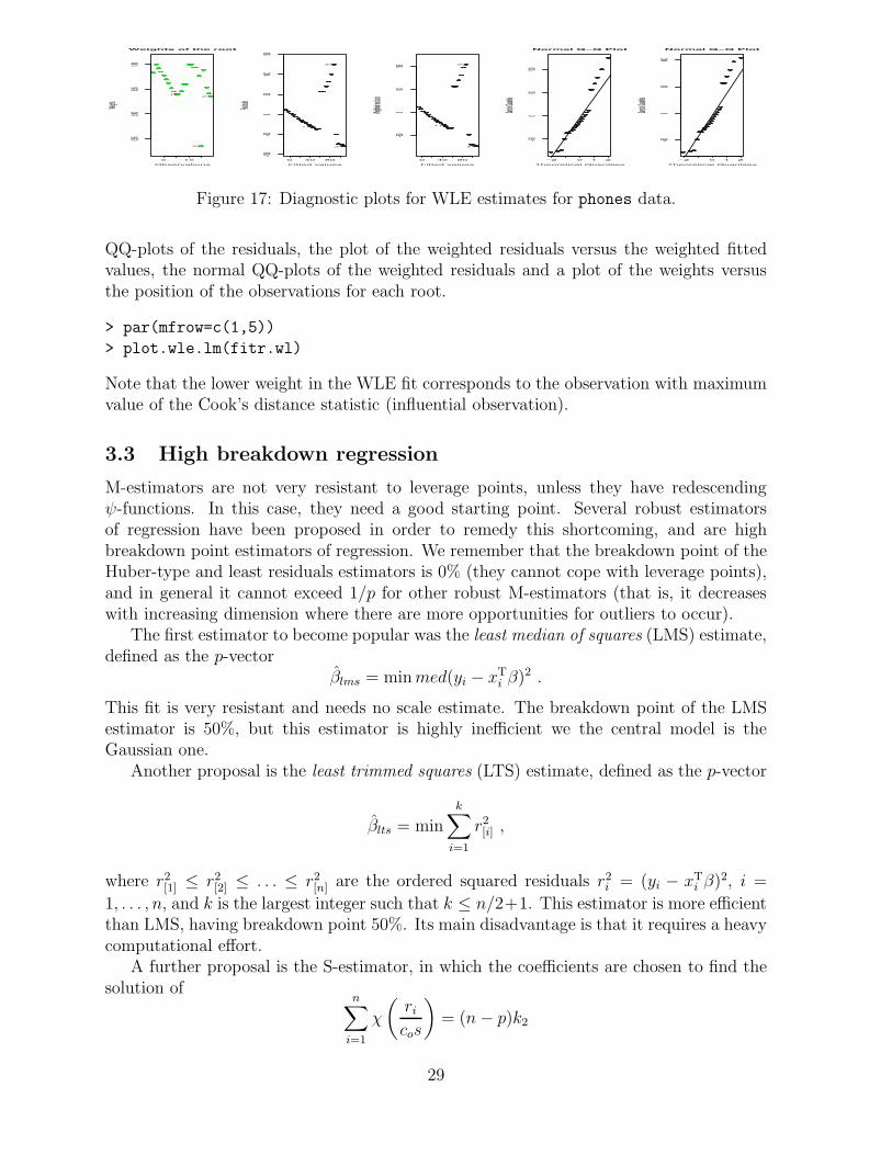
3.3 High breakdown regression
M-estimators are not very resistant to leverage points, unless they have redescending&-functions. In this case, they need a good starting point. Several robust estimatorsof regression have been proposed in order to remedy this shortcoming, and are highbreakdown point estimators of regression. We remember that the breakdown point of theHuber-type and least residuals estimators is 0% (they cannot cope with leverage points),and in general it cannot exceed 1/p for other robust M-estimators (that is, it decreaseswith increasing dimension where there are more opportunities for outliers to occur).
The first estimator to become popular was the least median of squares (LMS) estimate,defined as the p-vector
(lms = min med(yi " xTi ()2 .
This fit is very resistant and needs no scale estimate. The breakdown point of the LMSestimator is 50%, but this estimator is highly ine"cient we the central model is theGaussian one.
Another proposal is the least trimmed squares (LTS) estimate, defined as the p-vector
(lts = mink%
i=1
r2[i] ,
where r2[1] ) r2
[2] ) . . . ) r2[n] are the ordered squared residuals r2
i = (yi " xTi ()2, i =
1, . . . , n, and k is the largest integer such that k ) n/2+1. This estimator is more e"cientthan LMS, having breakdown point 50%. Its main disadvantage is that it requires a heavycomputational e!ort.
A further proposal is the S-estimator, in which the coe"cients are chosen to find thesolution of
n%
i=1
'
"ri
cos
$= (n " p)k2
29

with smallest scale s. Usually, '(·) is usually chosen to the integral of Tukey’s bisquarefunction, c0 = 1.548 and k2 = 0.5 is chosen for consistency at the Gaussian distribution.S-estimates have breakdown point 50%, such as for the bisquare family. However, theasymptotic e"ciency of an S-estimate under normal errors is 0.29, which is not verysatisfactory but is better than LMS and LTS.
It is possible to combine the resistance of these high breakdown estimators with thee"ciency of M-estimation. The MM-estimates (see Yohai, 1987, and Marazzi, 1993) havean asymptotic e"ciency as close to one as desired, and simultaneously breakdown point50%. Formally, the MM-estimate (MM it consists in: (1) compute an S-estimate withbreakdown point 1/2, denoted by ("; (2) compute the residuals r"i = yi"xT
i (" and find !"
solution of!n
i=1 '(r"i /!) = k2(n"p); (3) find the minimum (MM of!n
i=1 )((yi"(Txi)/!"),where )(·) is a suitable function. The function rlm has an option that allows to implementMM-estimation:
rlm(formula, data, ...,method="MM")
To use other breakdown point estimates, in R there exists the function lqs to fit aregression model using resistant procedures, that is achieving a regression estimator witha high breakdown point (see Rousseeuw and Leroy, 1987, Marazzi, 1993, and Venablesand Ripley, 2002, Sec. 6.5). The usage of the function lqs is:
lqs(formula, data, method = c("lts", "lqs", "lms", "S"),...)
where
• formula: is a formula of the form lm;
• data: (optional) is the data frame used in the analysis;
• method: the method to be used for resistant regression. The first three methodsminimize some function of the sorted squared residuals. For methods lqs and lmsis the quantile squared residual, and for lts it is the sum of the quantile smallestsquared residuals.
Several other arguments are available for this function, such as the tuning constant k0used for '(·) and &(·) functions when method = "S", currently corresponding to Tukey’sbiweight.
For summarizing the output of function lqs the function summary cannot be used.Function lqs gives a list with usual components, such as coefficients, scale residuals,fitted.values. In particular, scale gives the estimate(s) of the scale of the error. Thefirst is based on the fit criterion. The second (not present for method == "S") is basedon the variance of those residuals whose absolute value is less than 2.5 times the initialestimate. Finally, we remember that high breakdown procedures do not usually providestandard errors. However, these can be obtained by a data-based simulation, such as abootstrap.
Example: stackloss data
Consider again the dataset with n = 21 observations on p = 4 variables about operationaldata of a plant for the oxidation of ammonia to nitric acid, and let us complete the analysisby including also high breakdown point estimators.
30

> data(stackloss)> fit1 <- lqs(stack.loss ~ ., data = stackloss)> fit2 <- lqs(stack.loss ~ ., data = stackloss, method = "S")> fitmm <- rlm(stack.loss ~ ., data = stackloss, method = "MM")> fit1$coefficients(Intercept) Air.Flow Water.Temp Acid.Conc.-32.41826923 0.75000000 0.32692308 -0.03846154> fit2$coefficients(Intercept) Air.Flow Water.Temp Acid.Conc.-35.37610619 0.82522124 0.44247788 -0.07964602> fitmm$coefficients(Intercept) Air.Flow Water.Temp Acid.Conc.-41.7072683 0.9372710 0.5940631 -0.1129477> fit.hub$coefficients
(Intercept) stackloss[, 1] stackloss[, 2] stackloss[, 3]-41.0265311 0.8293739 0.9261082 -0.1278492
> fit.bis$coefficients(Intercept) stackloss[, 1] stackloss[, 2] stackloss[, 3]-42.2852537 0.9275471 0.6507322 -0.1123310
> fit1$scale[1] 0.9393087 1.0371971> fit2$scale[1] 1.911955> fitmm$s[1] 1.982660> fit.hub$s
112.440714> fit.bis$s
112.281886
Figure 18 compares the plots of the residuals versus fitted values for several fits. Figure19 gives the normal QQ-plots of the residuals of several fits for the stackloss data: theOLS residuals and residuals from high breakdown regression.
> par(mfrow=c(1,3))> plot(fit1$fit,fit1$res,main="LQS")> plot(fit2$fit,fit2$res,main="S")> plot(fitmm$fit,fitmm$res,main="MM")> par(mfrow=c(1,4))> fit <- lm(stack.loss ~ ., data = stackloss)> qqnorm(residuals(fit),main="LS")> qqline(residuals(fit))> qqnorm(residuals(fit1),main="LQS")> qqline(residuals(fit1))> qqnorm(residuals(fitmm),main="MM")> qqline(residuals(fitmm))
31

> qqnorm(residuals(fit2),main="S")> qqline(residuals(fit2))
10 20 30
!50
510
LQS
fit1$fit
fit1$
res
10 20 30
!10
!50
5
S
fit2$fit
fit2$
res
5 15 25 35
!10
!50
5
MM
fitmm$fit
fitm
m$r
es
Figure 18: Residuals versus fitted values for several residuals for stackloss data.
In this data set bad leverage points are not present and, in general, all the results ofthe di!erent robust fits are quite similar. Next Section will present an example in whichthe importance of high breakdown estimation emerges.
3.4 Bounded-influence estimation in linear regression models
The previous examples were based on some well-developed R libraries. We now presentsome further examples describing also some methods not implemented yet.
Huber type M-estimation of linear regression coe"cients does not provide bounded-influence estimation, as the influence function of the estimators is bounded in the y space(direction) but not in the x space. A remedy to this is given by bounded-influence es-timators, which use suitable weights on the design (x-weights). Here we consider bothMallows-type and Schweppe-type estimators, which can be obtained by suitable specifi-cation of the weights wi in (7). Two commonly used methods are the Mallows estimatorand the Hampel and Krasker estimator (see Hampel et al., 1986, §6.3). They are bothimplemented by our simple function lm.BI, which uses the & function given by the Hu-ber function (4). It implements an iterated weighted least squares algorithm followingJørgensen (1984), with ! updating and standard errors computed as in Street et al. (1988).The function has the following usage
lm.BI(beta.in, sigma.in, X, y, method, k1, k2, maxiter, mytol)
The arguments of the function lm.BI are
• beta.in, sigma.in: initial values for ( and !;
• X, y: design matrix and response vector;
• method: one of "huber", "mallows" or "hampel", implementing Huber, Mallows orHampel-Krasker regression. For Mallows regression, the x-weights wi = (1 " hii)1/2
are used, where hii is the i-th diagonal value of the hat matrix; for Hampel andKrasker regression the x-weights are obtained according to the formulas given in
32

!2 0 2
!60
4
LS
Theoretical Quantiles
Sam
ple
Qua
ntile
s
!2 0 2
!55
LQS
Theoretical Quantiles
Sam
ple
Qua
ntile
s
!2 0 2
!10
05
MM
Theoretical Quantiles
Sam
ple
Qua
ntile
s
!2 0 2
!10
05
S
Theoretical Quantiles
Sam
ple
Qua
ntile
s
Figure 19: Normal QQ-plots for several residuals for stackloss data.
Krasker and Welsch (1982). For Huber regression, the scale is estimated by HuberProposal 2, and for Mallows regression by a weighted version of the same method(Marazzi, 1993).
• k1, k2: tuning constants for regression and scale estimation. For Hampel andKrasker regression, k2 is not used. Default value for k1 is 1.345 (for Huber andMallows method) or 4.2 (for Hampel method).
• maxiter, mytol: maximum number of iterations and tolerance for the algorithm.
The function returns a list with several components, including:
• coef, s: parameter estimates;
• se, V: estimated standard errors and asymptotic variance matrix for the regressioncoe"cients;
• weights, fitted.values, residuals: vector of weights on the residuals, fittedvalues and (unstandardized) residuals.
The weights returned by the function are given by &k(ri/vi)/(ri/vi), i = 1, . . . , n, whereri are the standardized residuals and the vis are given by the function v(xi) of Kraskerand Welsch (1982) for the Hampel and Krasker estimator, and are 1 for the other meth-ods. They can play an important role for diagnostic purposes, as shown in the followingexamples.
33

Example: U.S. Mortality Data
As an example, we consider the US mortality data, already analysed by several authors,including Krasker and Welsch (1982). The data consist of n = 60 observations aboutage-adjusted mortality for a sample of U.S. cities, with several available covariates. Thedata are contained in the file mortality.txt.
> mort <- read.table("mortality.txt", T)> mort$logSOD <- log(mort$SOD)
For the sake of simplicity, we consider the same subset of covariates already selectedby Krasker and Welsch, namely percent nonwhite (NONW), average years of education(EDUC), population per square mile (DENS), precipitation (PREC) and a pollution variable(log(SOD)). The related scatterplots are shown in Figure 20.
> pairs(mort[,c(16,9,6,8,1,17)], panel = "panel.smooth")
MORT
0 10 30 2000 6000 10000 0 2 4
800
950
1100
010
30
NONW
EDUC
9.0
10.5
12.0
2000
6000
1000
0
DENS
PREC
1030
50
800 950 1100
02
4
9.0 10.5 12.0 10 30 50
logSOD
Figure 20: Mortality data: Scatterplots
We start the analysis with the OLS fit
> mort.ols <- lm(MORT ~ NONW + EDUC + DENS + PREC + log(SOD), data=mort)> summary(mort.ols)
....
34

Coefficients:Estimate Std. Error t value Pr(>|t|)
(Intercept) 930.282998 96.150153 9.675 2.17e-13NONW 3.349968 0.588559 5.692 5.29e-07EDUC -13.296076 6.969107 -1.908 0.061733DENS 0.002833 0.003758 0.754 0.454249PREC 1.637312 0.615956 2.658 0.010315log(SOD) 13.778244 3.815138 3.611 0.000668
....Residual standard error: 36.39 on 54 degrees of freedomMultiple R-Squared: 0.6868, Adjusted R-squared: 0.6578
Figure 21 show four diagnostic plots based on the OLS fit. In particular, the two upperpanels show a plot of residuals yi " µO
i versus fitted values µOi , with µO
i = xTi (OLS,
and normal Q-Q plot of standardized residuals, respectively; these are two of the plotsroutinely provided by the plot.lm function. The two lower panels show a plot of Cook’sstatistics against hii/(1"hii) and case plot of Cook statistics. The two latter plots can beobtained, for example, by means of the glm.diag.plots in the library boot. We followthis latter function, and add to the plots the same lines usually drawn by glm.diag.plotsto identify extreme values. More precisely, the threshold for Cook statistic is set at8/(n " 2p). Points above this line may be points with high influence on the model. Forleverage points, the threshold is at 2p/(n " 2p) and points beyond this value have highleverage compared to the variance of the raw residual at that point. From the plots, it isapparent that there are several high-leverage points, which in some cases are associatedto large residuals, thus originating influential points.
> par(mfrow=c(2,2), pty = "s")> plot.lm(mort.ols, which = 1:2)> X.mort <- model.matrix(mort.ols)> h.mort <- hat(X.mort)> c.mort <- cooks.distance(mort.ols)> plot(h.mort / (1 - h.mort), c.mort, xlab = "h/(1-h)", ylab = "Cook statistic")> abline(h = 8 / (nrow(X.mort) - 2 * mort.ols$rank), lty = 2)> abline(v = (2 * mort.ols$rank) / (nrow(X.mort)- 2 * mort.ols$rank), lty = 2)> plot(c.mort,xlab = "Case", ylab = "Cook statistic")> abline(h = 8 / (nrow(X.mort) - 2 * mort.ols$rank), lty = 2)
We start the robust analysis by getting Huber-regression estimates. Note that the Huberestimates provided lm.BI are quite similar to those returned by rlm using Huber Proposal2 for the scale, although there are some slight di!erences for standard errors.
> s.est <- sqrt(mean(mort.ols$res^2))> mort.hub <- lm.BI(mort.ols$coef, s.est, X.mort, mort$MORT, "huber", 1.345,
1.5)> tab.hub <- cbind(mort.ols$coef, mort.hub$coef, sqrt(diag(vcov(mort.ols))),
mort.hub$se)> colnames(tab.hub) <- c("OLS coef", "HUB coef", "OLS se", "HUB se")> print(tab.hub, digits=3)
OLS coef HUB coef OLS se HUB se
35

850 900 950 1050!1
000
5010
0
Fitted values
Resid
uals
Residuals vs Fitted
37
28
2
!2 !1 0 1 2
!3!1
01
23
4
Theoretical Quantiles
Stan
dard
ized
resid
uals
Normal Q!Q plot
37
2832
0.0 0.2 0.4 0.6
0.0
0.2
0.4
0.6
h/(1!h)
Cook
sta
tistic
0 10 20 30 40 50 600.
00.
20.
40.
6
Case
Cook
sta
tistic
Figure 21: Mortality data: Diagnostic plots for OLS estimates
(Intercept) 930.28300 915.74868 96.15015 82.41696NONW 3.34997 2.83928 0.58856 0.50450EDUC -13.29608 -12.94116 6.96911 5.97370DENS 0.00283 0.00396 0.00376 0.00322PREC 1.63731 1.86757 0.61596 0.52798log(SOD) 13.77824 14.89441 3.81514 3.27022
One of the main use of robust regression is for diagnostic purposes. To this end, wecan compare the classical OLS-based diagnostics with the Huber weights. In particular,we compare the Huber weights with hii/(1 " hii), the Cook’s statistics and the DFFITstatistic (Belsley et al., 1980), defined as DFFIT= (yi " µO
i )*
hii/{s(i) (1"hii)}, with s(i)
is the estimate of ! after dropping the i-th observation. See Figure 22. Although all thepoints associated with high values of the classical statistics have a Huber weight less then1, there are also some observations with a low Huber weight which were not identified bythe classical diagnostics.
> plot(mort.hub$weights, xlab="Case", ylab="Huber weight")> plot(h.mort / (1-h.mort), mort.hub$weights, xlab = "h/(1-h)",
ylab = "Huber weight")> abline(v = (2 * mort.ols$rank) / (nrow(X.mort) - 2 * mort.ols$rank), lty=2)> plot(c.mort, mort.hub$weights, xlab = "Cook statistic", ylab = "Huber weight")
36

> abline(v = 8 / (nrow(X.mort) - 2 * mort.ols$rank), lty = 2)> df.mort <- dffits(mort.ols)> plot(df.mort, mort.hub$weights, xlab = "DFFIT", ylab = "Huber weight")
0 10 20 30 40 50 60
0.4
0.6
0.8
1.0
Case
Hube
r wei
ght
0.0 0.2 0.4 0.6
0.4
0.6
0.8
1.0
h/(1!h)
Hube
r wei
ght
0.0 0.2 0.4 0.6
0.4
0.6
0.8
1.0
Cook statistic
Hube
r wei
ght
!2 !1 0 1 2
0.4
0.6
0.8
1.0
DFFIT
Hube
r wei
ght
Figure 22: Mortality data: Comparison between OLS-based and Huber-based diagnostics
It is also interesting to look at some residual plots based on the Huber estimates. Afterhaving defined the fitted values µH
i = xTi (Huber and the residuals yi " µH
i , we obtain theplot of residuals versus fitted values and a normal Q-Q plot of standardized residuals.They are reported in Figure 23.
> plot(mort.hub$fit, mort.hub$res, xlab = "Fitted values", ylab = "Residuals",main = "Residuals vs Fitted")
> points(mort.hub$fit[mort.hub$we < 1], mort.hub$res[mort.hub$we < 1], col=2)> qqnorm(mort.hub$res / mort.hub$s, main = "Normal Q-Q plot of residuals")> qqline(mort.hub$res / mort.hub$s)
We now turn to bounded-influence estimation, and fit both the Mallows and the Ham-pel and Krasker estimator. We use the same values of the tuning constants selected byKrasker and Welsch (1982), hence setting k1=1.345 and k1=4.2 respectively, and achiev-ing roughly the same amount of weighting in both cases.
mort.mal<- lm.BI(mort.ols$coef, s.est, X.mort, mort$MORT, "mallows", 1.345,
37

850 950 1050
!100
!50
050
100
Residuals vs Fitted
Fitted values
Resid
uals
!2 !1 0 1 2
!3!1
01
23
4
Normal Q!Q plot of residuals
Theoretical Quantiles
Sam
ple
Qua
ntile
s
Figure 23: Mortality data: Diagnostic plots for Huber estimates
1.5)mort.hk<- lm.BI(mort.ols$coef, s.est, X.mort, mort$MORT, "hampel", 4.2)
Let us have a look at the di!erent estimates.
> tab.bi <- cbind(mort.ols$coef, mort.mal$coef, mort.hk$coef,sqrt(diag(vcov(mort.ols))), mort.mal$se, mort.hk$se)
> colnames(tab.bi) <- c("OLS coef", "MAL coef", "H-K coef", "OLS se","MAL se", "H-K se")
> print(tab.bi, digits=3)OLS coef MAL coef H-K coef OLS se MAL se H-K se
(Intercept) 930.28300 915.63660 915.40807 96.15015 81.39012 85.35153NONW 3.34997 2.80715 2.59896 0.58856 0.49797 0.51438EDUC -13.29608 -13.17073 -13.68873 6.96911 5.90093 6.18970DENS 0.00283 0.00509 0.00716 0.00376 0.00319 0.00341PREC 1.63731 1.89309 2.01018 0.61596 0.52120 0.54165log(SOD) 13.77824 14.35093 13.59010 3.81514 3.23012 3.39482
Both the Mallows estimates and the Hampel and Krasker ones seem to deviate fromthe OLS results, but the direction of the adjustment is di!erent for some coe"cients.Standard errors are generally smaller for robust methods, due to smaller estimate of thescale parameter !. More precisely, the di!erent estimated scales are given by
> tab.sigma <- c(s.est, mort.hub$s, mort.mal$s, mort.hk$s)> names(tab.sigma) <- c("OLS", "HUB", "MAL", "H-K")> print(tab.sigma, digits=4)
OLS HUB MAL H-K34.52 31.17 30.50 29.90
38

It may be useful to compare the weighting action performed by the various methods. Tothis end, we can compare the weights for those observations where one the method gavea weight smaller than 1.
> w.mort <- cbind(mort.hub$weights, mort.mal$weights, mort.hk$weights)> cond <- apply(w.mort, 1, "<",1)> cond <- apply(cond, 2, sum)> w.mort[(cond>0),]
[,1] [,2] [,3]2 0.5398001 0.5349548 1.00000006 1.0000000 1.0000000 0.89259949 0.8067073 0.8480886 0.992354228 0.4124823 0.4018182 0.383022131 1.0000000 1.0000000 0.950485832 0.5642053 0.5265649 0.293061335 0.9703016 0.9788623 1.000000037 0.3482611 0.3453883 0.220626053 0.8466948 0.8257080 1.000000057 0.8836090 0.8569866 1.000000059 0.5524462 0.4915569 0.1865103
All the three methods tend to downweight the observations in a similar fashion, but thereare some di!erences.
We now turn to some of the high-breakdown methods introduced in the previoussections. First we compute the MM-estimate using the function rlm
> mort.MM<- rlm(MORT ~ NONW + EDUC + DENS + PREC + log(SOD), data=mort,method="MM")
> summary(mort.MM, corr=F)....
Coefficients:Value Std. Error t value
(Intercept) 904.1765 85.6275 10.5594NONW 2.5952 0.5241 4.9513EDUC -11.9896 6.2064 -1.9318DENS 0.0025 0.0033 0.7337PREC 1.8681 0.5485 3.4055log(SOD) 17.6414 3.3976 5.1923Residual standard error: 29.47 on 54 degrees of freedom
Another possibility is to use the weighted-likelihood estimating equations approach im-plemented by the library wle.
> mort.wle <- wle.lm(MORT ~ NONW + EDUC + DENS + PREC + log(SOD),data=mort, num.sol=10)
> summary(mort.wle)....
Coefficients:Estimate Std. Error t value Pr(>|t|)
39

(Intercept) 891.369970 85.921397 10.374 2.98e-14NONW 2.651674 0.530454 4.999 6.95e-06EDUC -10.425735 6.251666 -1.668 0.10141DENS 0.001109 0.003260 0.340 0.73513PREC 1.781121 0.531708 3.350 0.00151log(SOD) 18.691913 3.500043 5.340 2.08e-06Residual standard error: 31.18 on 51.86464 degrees of freedom
Both the two high-breakdown methods give similar results. A more thorough summary ofall the results for this example can be obtained by plotting the Wald statistics (k/se((k)for the various coe"cients, as shown in Figure 24.
> par(mfrow=c(2,3), pty="s", cex=0.8)> for(i in 1:6)> { vet<-c(mort.ols$coef[i] / sqrt(diag(vcov(mort.ols)))[i],
mort.hub$coef[i] / mort.hub$se[i],> mort.mal$coef[i] / mort.mal$se[i],
mort.hk$coef[i] / mort.hk$se[i],> mort.MM$coef[i] / sqrt(diag(vcov(mort.MM)))[i],
mort.wle$coef[i] / mort.wle$sta[i])> names(vet)<-c("OLS", "HUB", "MAL", "H-K", "MM", "WLE")> dotchart(vet, main=names(mort.ols$coef)[i], cex=1)}
Example: Artificial Data
This data set was generated by Hawkins et al. (1984) for illustrating some of the meritsof a robust technique. The data set consists of n = 75 observations in four dimensions(one response and three explanatory variables). The first 10 observations are bad leveragepoints, and the next four points are good leverage points (see also Rousseeuw and Leroy,1987).
An exploratory graphical analysis can be made using the fancy scatterplots providedby the function scatterplot.matrix in the library car (see Figure 25). In this case, forall the variables considered, the presence of the bad and good leverage points is clearlynoticeable.
> library(wle)> data(artificial)> scatterplot.matrix(artificial)
We get some useful indications from some plots of residuals versus fitted values, shownin Figure 26.
> art.ols <- lm(y ~ x1 + x2 + x3, artificial)> summary(art.ols)
....Coefficients:
Estimate Std. Error t value Pr(>|t|)
40

OLSHUBMALH!KMMWLE
10.0 10.5 11.0
(Intercept)
OLSHUBMALH!KMMWLE
5.0 5.2 5.4 5.6
NONW
OLSHUBMALH!KMMWLE
!2.2 !2.0 !1.8
EDUC
OLSHUBMALH!KMMWLE
0.5 1.0 1.5 2.0
DENS
OLSHUBMALH!KMMWLE
2.8 3.2 3.6
PREC
OLSHUBMALH!KMMWLE
4.0 4.5 5.0
log(SOD)
Figure 24: Mortality data: Comparison of Wald statistics
(Intercept) -0.3934 0.4106 -0.958 0.34133x1 0.2492 0.2580 0.966 0.33731x2 -0.3354 0.1550 -2.164 0.03380x3 0.3808 0.1281 2.974 0.00402
....Residual standard error: 2.249 on 71 degrees of freedomMultiple R-Squared: 0.6024, Adjusted R-squared: 0.5856> par(mfrow=c(1,2), pty="s")> plot(art.ols$fit, art.ols$res, xlab = "Fitted values", ylab = "Residuals",
main = "OLS fit")> art.hub <- lm.BI(art.ols$coef, mean(art.ols$res^2), model.matrix(art.ols),
artificial$y, "huber", 1.345, 1.5)> art.mal <- lm.BI(art.ols$coef, mean(art.ols$res^2), model.matrix(art.ols),
artificial$y, "mallows", 1.345, 1.5)> plot(art.mal$fit, art.mal$res, xlab = "Fitted values", ylab = "Residuals",
main= "Mallows fit")
The 14 high-leverage points are clearly noticeable with both OLS and robust estimation,as they form two rather distinct clusters. However, due to the e!ect of influential obser-vations on the fit, now the role of good and bad leverage points has been totally reversed.This fact is even more apparent for the Mallows estimate. Here only high-breakdownestimation is capable of correctly identify the bad leverage points. For example, let ustry the weighted likelihood approach. The summary reveals that wle.lm has found two
41

|| ||| ||||| | |||||| || ||| |||| |||| || || ||| | || ||| ||| ||||| || || || |||| || ||| || || |||||
x1
0 5 15 25 35 0 2 4 6 8 10
02
46
810
05
1525
35||| ||||||| || | ||||| ||||||| ||||||||| ||||| ||| ||||| |||||| |||| ||| || ||||||| ||||||
x2
|| |||||| || | |||||| |||||||| |||| ||||| |||||| ||| || || ||||| |||||| ||||| |||||| ||||||
x3
010
2030
0 2 4 6 8 10
02
46
810
0 10 20 30
|||| || |||||| ||| ||||| ||| |||| ||||||| ||| ||||| ||||| | || || |||| |||| | ||| ||| || ||| || |
y
Figure 25: Artificial data: Scatterplots
roots of the estimating equations.
> art.wle <- wle.lm(y.artificial ~ x.artificial, boot = 40, num.sol = 3)....
Root 1Coefficients:
Estimate Std. Error t value Pr(>|t|)(Intercept) -0.94351 0.12792 -7.376 3.46e-10x.artificial1 0.15653 0.07809 2.005 0.049112x.artificial2 0.18912 0.07168 2.638 0.010382x.artificial3 0.18152 0.05021 3.615 0.000581---Residual standard error: 0.6688 on 66.03095 degrees of freedom
....Root 2Coefficients:
Estimate Std. Error t value Pr(>|t|)(Intercept) -0.19670 0.10419 -1.888 0.064 .x.artificial1 0.08969 0.06655 1.348 0.183x.artificial2 0.03875 0.04076 0.951 0.346x.artificial3 -0.05298 0.03549 -1.493 0.141---Residual standard error: 0.5561 on 58.6243 degrees of freedom
The residual versus fitted values plots corresponding to the two roots are readily obtained
42

0 2 4 6 8
!8!4
02
4
OLS fit
Fitted values
Resid
uals
0 2 4 6 8 10 12
!12
!8!4
02
Mallows fit
Fitted values
Resid
uals
Figure 26: Artificial data: Residuals vs Fitted values
(Figure 27).
plot(art.wle$fit[1,], art.wle$res[1,], xlab = "Fitted values",ylab = "Residuals", main = "First root")
plot(art.wle$fit[2,], art.wle$res[2,], xlab = "Fitted values",ylab = "Residuals", main = "Second root")
The two plots are rather di!erent. While the one related to the first root looks quitesimilar to the one based on Mallows estimate, the second root gives a rather di!erentpicture. In particular, it correctly identifies the bad leverage points, and the fitted valuesare all around 0, as it should be due to the way the data were generated. The samehappens also with the MM-estimator. In fact, the MM-estimates obtained with rlm arevery close to the second wle.lm root, while the bounded-influence estimates are close tothe first one.
> art.MM <- rlm(y ~ x1 + x2 + x3, artificial, method="MM")> tab.coef <- cbind(art.ols$coef, art.mal$coef, art.hk$coef, art.MM$coef,
art.wle$coef[1,], art.wle$coef[2,])> colnames(tab.coef) <- c("OLS", "MAL", "H-K", "MM", "WLE-1", "WLE-2")> print(tab.coef, digits=3)
OLS MAL H-K MM WLE-1 WLE-2(Intercept) -0.393 -0.8293 -0.877 -0.1994 -0.944 -0.1967x1 0.249 0.1714 0.163 0.0960 0.157 0.0897x2 -0.335 0.0674 0.133 0.0405 0.189 0.0387x3 0.381 0.2377 0.204 -0.0565 0.182 -0.0530
43

0 2 4 6 8 10
!10
!50
First root
Fitted values
Resid
uals
!0.3 !0.1 0.1 0.3
02
46
810
Second root
Fitted values
Resid
uals
Figure 27: Artificial data: Residuals vs Fitted values for weighted likelihood estimates
> tab.se <- cbind(sqrt(diag(vcov(art.ols))), art.mal$se, art.hk$se,sqrt(diag(vcov(art.MM))), art.wle$sta[1,],art.wle$sta[2,])
> colnames(tab.se) <- c("OLS", "MAL", "H-K", "MM", "WLE-1", "WLE-2")> print(tab.se, digits=3)
OLS MAL H-K MM WLE-1 WLE-2(Intercept) 0.411 0.1526 0.1528 0.1154 0.1279 0.1042x1 0.258 0.0959 0.0952 0.0725 0.0781 0.0666x2 0.155 0.0585 0.0680 0.0436 0.0717 0.0408x3 0.128 0.0479 0.0518 0.0360 0.0502 0.0355
To wind up, this example show that sometimes bounded-influence estimation can giverather misleading results. Although this is an artificially extreme example, it suggests theimportant role played by high-breakdown estimation.
4 Bounded-influence estimation in logistic regression
There are several methods developed for logistic regression, like the Optimal Bias-RobustEstimator (OBRE) of Kunsch et al. (1989), the Bianco and Yohai estimator (1996) or theMallows-type estimator of Cantoni and Ronchetti (2001). Here we focus in particular onthe latter two proposals, noticing however that the ROBETH software (Marazzi, 1993)includes also several FORTRAN routines for the computation of the OBRE, some of whichhave been (partially) ported to R.
44

4.1 Mallows-type estimation
The Mallows-type estimator of Cantoni and Ronchetti (2001) is defined for the class ofgeneralized linear models. They defined some estimating equations which nicely extendthe likelihood equations. Such estimating equations can be written as
g((; y) =n%
i=1
w(xi){&k(ri) " a(µi)}
Vi(µi)1/2
*µi
*(
T
= 0 , (8)
where V (µi) is the variance function, ri = (yi " µi)/*
Vi the Pearson residuals and &k
the Huber function introduced in section 2.3. The non-random values a(µi) are definedas a(µi) = E[&k(Ri)|xi], and ensure the conditional Fisher-consistency of the estimatingequations. For binomial or Poisson response the computation of a(µi) is not di"cult,as reported in Cantoni and Ronchetti (2001). From general theory of M-estimation itfollows that the estimator (M defined as the solution of the equations g((; Y ) = 0 hasbounded influence function, as the e!ect of outlying values in the response is bounded bya finite value of the tuning constant k and the e!ect of outlying values in the covariates isbounded by a suitable choice of the weights w(xi) (Cantoni and Ronchetti, 2001). Notethat when k % & and w(xi) = 1, then a(µi) = 0 and g((; y) becomes the score function,hence the Maximum Likelihood Estimator (MLE) is a special case of (M .
An important special case of (8) is obtained with normal homoscedastic data andidentity link function, for which V (µi) = !2. The resulting model belong to the GLMclass for a fixed value of the scale parameter !. In this case, (M is a Mallows estimate forlinear regression, becoming the Huber estimate for w(xi) = 1.
Some S-PLUS functions for the solution of (8) are available (Cantoni 2004), which canbe used in R with some minor changes. A simple, direct implementation of the method isactually not di"cult, and we propose it in the following just for illustrative purposes.
The first step is to write a function for the computation of the estimating functiong((; y). For the particular case of logistic regression this can be done by considering thatµi = F (xT
i (), with F (u) = exp(u)/(1 + exp(u)), Vi(µi) = µi (1 " µi) = Vi and
a(µi) = &k
&(1 " µi)/
'Vi
(µi + &k
&"µi/
'Vi
((1 " µi) .
A simple function for computing g((; y) is readily written
g.fun <- function(beta, X, y, offset, w.x, k1){mu<- plogis(X %*% beta + offset)V <- mu * (1 - mu)r <- (y - mu) / sqrt(V)a <- psiHub((1 - mu) / sqrt(V), k1) * mu + psiHub(-mu / sqrt(V), k1)
* ( 1 - mu)colSums(X * as.vector(1 / sqrt(V) * w.x * (psiHub(r.stand, k1) - a) * V))}
where the function psiHub(x, k) = psi.huber(x, k) * x and k1 is the k constant.The solution of the equation g((; y) = 0 can be obtained in several ways, but the simplestpossibility is to implement a Newton-Rapshon algorithm, obtaining the Jacobian of g((; y)
45

by numerical di!erentiation. In our function logit.BI we use the simple numericalroutine num.deriv from the sn library. Hence, the updating of the beta coe"cientsis essentially performed by the commands
> g.old <- g.fun(beta.old, X, y, offset, w.x, k1)> J.old <- num.deriv(beta.old, "g.fun", X = X, y = y,
offset = offset, w.x = w.x, k1 = k1)> beta.new <- beta.old - qr.solve(J.old, g.old)
The logit.BI function has the following usage
logit.BI(beta.in, X, y, k1, offset, w.x, maxiter, mytol)
and the various arguments are:
• beta.in: initial value for (;
• X, y: design matrix, response vector;
• k1: tuning constant, default is 1.2.
• offset: o!set (default is a vector of 0s);
• w.x: x-based prior weights for Mallows estimation (default is a vector of 1s);
• maxiter, mytol: maximum number of iterations and tolerance for the algorithm.
The function returns a list with several components, including:
• coef: parameter estimates;
• se, V: estimated standard errors and asymptotic variance matrix for the regressioncoe"cients;
• weights: vector of weights on the residuals.
4.2 The Bianco and Yohai estimator
An alternative method is given by the Bianco and Yohai estimator (Bianco and Yohai,1996), defined as
(BY = argmin"
n%
i=1
))k(d(xT
i (; yi)) + C(xTi ()
*(9)
where d(u; y) = "y log F (u)" (1" y) log{(1" u)}, )k is a bounded function and C(xTi ()
is a bias correction term. Bianco and Yohai (1996) proposed the following ) function,
)k(x) =
+,-
,.
x " x2
2kif x ) k
k
2otherwise
46

but stressed that other choices are possible. Croux and Haesbroeck (2003) extend theBianco and Yohai estimator by including weights for downweighting high-leverage points,thus defining a bounded-influence estimator
(WBY = argmin"
n%
i=1
w(xi)))k(d(xT
i (; yi)) + C(xTi ()
*. (10)
They suggested a decreasing function of robust Mahalanobis distances for the weightsw(xi), where the distances are computed using the Minimum Covariance Determinant(MCD) estimator (see Rousseeuw and Leroy, 1987). More precisely, w(xi) are obtained asfollows. The MCD method seeks h points whose covariance has minimum determinant,and Croux and Haesbroeck (2003) suggest h = 3/4 n, giving a 25% breakdown pointestimator. The method is implemented by the function cov.rob (or cov.mcd, which is aconvenient wrapper) in the MASS library. If X is the design matrix, the robust estimate ofmultivariate location and scale are obtained by
> hp <- floor(nrow(X) * 0.75) + 1> mcdx <- cov.rob(X, quan = hp, method = "mcd")
Once the robust estimate of location and scale have been computed, we can obtain therobust distances RDi. Finally the weights are defined as w(xi) = W (RDi), where W isthe weight function W (t) = I{t2##2
p,0.975}, with IA denoting the indicator function of theset A.
> rdx <- sqrt(mahalanobis(X, center = mcdx$center, cov = mcdx$cov))> vc <- sqrt(qchisq(0.975, ncol(X)))> wx <- as.numeric(rdx <= vc)
Notice that the same weights could also be used in (8). Croux and Haesbroeck (2003) haveimplemented both the Bianco and Yohai estimator and their weighted version in somepublic-domain S-PLUS functions, which can be also used in R with a few changes. Thetwo functions are BYlogreg and WBYlogreg, respectively, which we slightly modified inorder to deal with dummy covariates in the design matrix. The arguments of the functionBYlogreg are
• x0, y: design matrix (not including the intercept), response vector;
• x0cont: design matrix to use for computing the weighted MLE (if initwml=T)
• initwml: logical value for selecting one of the two possible methods for computingthe initial value: if initwml=T a weighted MLE, otherwise the classical MLE.
• const: tuning constant, default is 0.5.
• kmax, maxhalf: maximum number of iterations and max number of step-halving.the algorithm.
The functions returns a list, including the components coef and sterror for parameterestimates and standard errors. The function WBYlogreg has exactly the same arguments,with the exception of initwml as the weighted MLE is always used as starting point.
47

Example: Food Stamp Data
This is a classical example of robust statistics, see for example Kunsch et al. (1989). Thefood stamp data set, of sample size 150, consists of a binary response variable participa-tion in the US Food Stamp Program. The covariates included in the model are tenancy(Tenancy), supplemental income (SupInc), and log(monthly income + 1) (log(Inc+1)).The data are contained in the file foodstamp.txt. Let us start the analysis by gettingthe MLE.
> food <- read.table("foodstamp.txt", T)> food.glm <- glm(y ~ Tenancy + SupInc + log(Inc+1), binomial, food)> summary(food.glm)
....Coefficients:
Estimate Std. Error z value Pr(>|z|)(Intercept) 0.9264 1.6229 0.571 0.56813Tenancy -1.8502 0.5347 -3.460 0.00054SupInc 0.8961 0.5009 1.789 0.07365log(Inc + 1) -0.3328 0.2729 -1.219 0.22280
The only significant coe"cient seems to be that of the variable tenancy. A look at somediagnostic plots is quite useful (see Figure 28).
> glm.diag.plots(food.glm)
It is clear that there is an observation with totally anomalous covariate values, which hasa very strong e!ect on the fit. In fact, observation 5 is the only one with a zero value forthe monthly income.
> food$Inc[1] 271 287 714 521 0 518 458 1266 350 168 235 450 683 519...
Any kind of robust method suitable for this data set must clearly bound the influenceof the design points. We get both the weights based on the hat matrix (used in theirexamples by Cantoni and Ronchetti, 2001), and those based on the robust estimation oflocation and scale. Following the suggestions in the code by Croux and Haesbroeck, inthe latter case we compute the weights using only the continuous covariate.
> X.food <- model.matrix(food.glm)> w.hat.food <- sqrt(1 - hat(X.food))> hp.food <- floor(nrow(X.food) * 0.75) + 1> mcdx.food <- cov.mcd(as.matrix(X.food[,-(1:3)]), quan = hp.food, method = "mcd")> rdx.food <- sqrt(mahalanobis(as.matrix(X.food[,-(1:3)]),
center = mcdx.food$center, cov = mcdx.food$cov))> vc.food <- sqrt(qchisq(0.975, 1))> w.rob.food <- as.numeric(rdx.food <= vc.food)
The two sets of weights present some di!erences, and the hat matrix-based ones providea smaller degree of weighting
48

!3 !2 !1 0 1
!2!1
01
2
Linear predictor
Resid
uals
!2 !1 0 1 2
!2!1
01
2
Ordered deviance residuals
Qua
ntile
s of
sta
ndar
d no
rmal
0.0 0.2 0.4 0.6 0.8 1.0
0.0
0.5
1.0
1.5
h/(1!h)
Cook
sta
tistic
0 50 100 150
0.0
0.5
1.0
1.5
Case
Cook
sta
tistic
Figure 28: Foodstamp data: diagnostic plots for maximum likelihood estimates
> mean(w.rob.food)[1] 0.94> mean(w.hat.food)[1] 0.9864798
However, both types of weight reach their minimum value at the observation 5. We nowcompute the robust estimates (M , including a Huber-type version without any prior x-weights. We start the algorithm from the MLE and, following Cantoni and Ronchetti(2001), we set k = 1.2.
> food.hub <- logit.BI(food.glm$coef, X.food, food$y, 1.2,)> food.mal <- logit.BI(food.glm$coef, X.food, food$y, 1.2, w.x = w.hat.food)> food.mal.wrd <- logit.BI(food.glm$coef, X.food, food$y, 1.2, w.x = w.rob.food)> tab.coef <- (cbind(food.glm$coef, food.hub$coef, food.mal$coef, food.mal.wrd$coef))> colnames(tab.coef)<- c("MLE", "HUB", "MAL-HAT", "MAL-ROB")> print(tab.coef, digits = 3)
MLE HUB MAL-HAT MAL-ROB(Intercept) 0.926 0.710 6.687 8.065Tenancy -1.850 -1.778 -1.855 -1.784SupInc 0.896 0.802 0.606 0.586log(Inc + 1) -0.333 -0.287 -1.298 -1.540
49
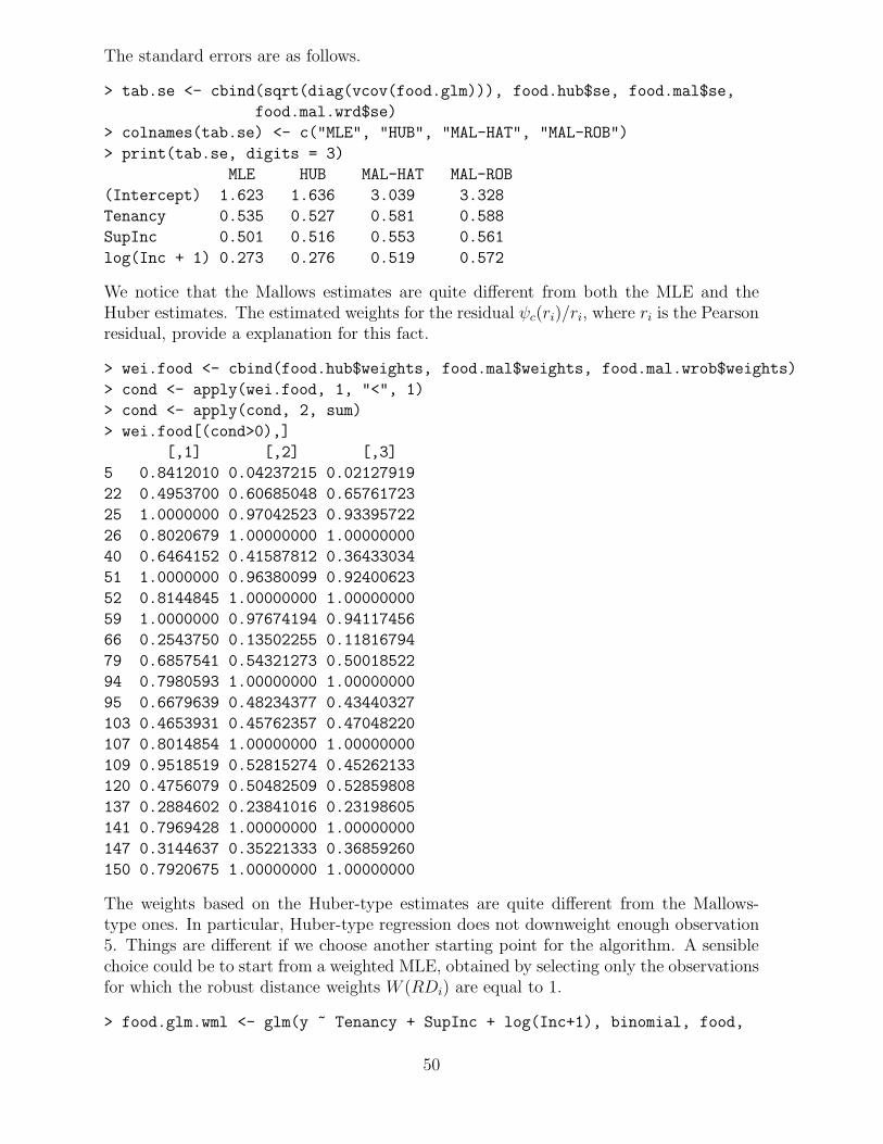
The standard errors are as follows.
> tab.se <- cbind(sqrt(diag(vcov(food.glm))), food.hub$se, food.mal$se,food.mal.wrd$se)
> colnames(tab.se) <- c("MLE", "HUB", "MAL-HAT", "MAL-ROB")> print(tab.se, digits = 3)
MLE HUB MAL-HAT MAL-ROB(Intercept) 1.623 1.636 3.039 3.328Tenancy 0.535 0.527 0.581 0.588SupInc 0.501 0.516 0.553 0.561log(Inc + 1) 0.273 0.276 0.519 0.572
We notice that the Mallows estimates are quite di!erent from both the MLE and theHuber estimates. The estimated weights for the residual &c(ri)/ri, where ri is the Pearsonresidual, provide a explanation for this fact.
> wei.food <- cbind(food.hub$weights, food.mal$weights, food.mal.wrob$weights)> cond <- apply(wei.food, 1, "<", 1)> cond <- apply(cond, 2, sum)> wei.food[(cond>0),]
[,1] [,2] [,3]5 0.8412010 0.04237215 0.0212791922 0.4953700 0.60685048 0.6576172325 1.0000000 0.97042523 0.9339572226 0.8020679 1.00000000 1.0000000040 0.6464152 0.41587812 0.3643303451 1.0000000 0.96380099 0.9240062352 0.8144845 1.00000000 1.0000000059 1.0000000 0.97674194 0.9411745666 0.2543750 0.13502255 0.1181679479 0.6857541 0.54321273 0.5001852294 0.7980593 1.00000000 1.0000000095 0.6679639 0.48234377 0.43440327103 0.4653931 0.45762357 0.47048220107 0.8014854 1.00000000 1.00000000109 0.9518519 0.52815274 0.45262133120 0.4756079 0.50482509 0.52859808137 0.2884602 0.23841016 0.23198605141 0.7969428 1.00000000 1.00000000147 0.3144637 0.35221333 0.36859260150 0.7920675 1.00000000 1.00000000
The weights based on the Huber-type estimates are quite di!erent from the Mallows-type ones. In particular, Huber-type regression does not downweight enough observation5. Things are di!erent if we choose another starting point for the algorithm. A sensiblechoice could be to start from a weighted MLE, obtained by selecting only the observationsfor which the robust distance weights W (RDi) are equal to 1.
> food.glm.wml <- glm(y ~ Tenancy + SupInc + log(Inc+1), binomial, food,
50

subset = (w.rob.food==1))Coefficients:
Estimate Std. Error z value Pr(>|z|)(Intercept) 5.6408 2.7665 2.039 0.041452Tenancy -1.7749 0.5352 -3.317 0.000911SupInc 0.6491 0.5181 1.253 0.210238log(Inc + 1) -1.1123 0.4685 -2.374 0.017589
If we recompute the algorithm form the weighted MLE, the Huber-type estimates areclose to the Mallows one, and the weight given to observation 5 is now much smaller.
> food.hub.wml <- logit.BI(food.glm.wml$coef, X.food, food$y, 1.2)> food.hub.wml$coef(Intercept) Tenancy SupInc log(Inc + 1)
6.531852 -1.847610 0.607605 -1.270387> food.hub.wml$weights[5]
50.04579391
A similar result is obtained with the Bianco and Yohai estimator. If we call the BYlogregwith the argument initwml = F, the MLE is used as starting point.
> food.BY<- BYlogreg(X.food[,-1], food$y, initwml = F)> food.BY
....$coef
(Intercept) x0Tenancy x0SupInc x0log(Inc + 1)[1,] 0.8814444 -1.768291 0.8456321 -0.3218968$sterror
Tenancy SupInc log(Inc + 1)5.7102449 0.5785001 0.6279328 0.9294853
The results are not much di!erent from the MLE. A better option is to use the weightedMLE as starting point. This requires as a further argument the matrix used to computethe weights.
> food.BY.wml <- BYlogreg(X.food[,-1], food$y, as.matrix(X.food[,-(1:3)]))> food.BY.wml
....$coef
(Intercept) x0Tenancy x0SupInc x0log(Inc + 1)[1,] 5.369783 -1.691211 0.6173553 -1.070233$sterror
Tenancy SupInc log(Inc + 1)7.0927687 0.5391049 0.5240751 1.2190520
The results are similar to the weighted version of the Bianco and Yohai estimator.
> food.WBY <- WBYlogreg(X.food[,-1], food$y, as.matrix(X.food[,-(1:3)]) )>food.WBY
51

....$coef
(Intercept) subx01 subx02 subx03[1,] 5.824949 -1.832782 0.6703187 -1.148582$sterror[1] 3.3923786 0.5822091 0.5220386 0.5906120
In order to compare all the various estimates, we follow the approach of Kordzakhiaet al. (2001). They proposed to compare the various estimates using a goodness-of-fitdiscrepancy, the chi-square statistic based on the arcsin transformation
X2arc =
n%
i=1
4&arcsin
*yi " arcsin
'%i
(,
where*%i are the fitted probabilities. The values of the statistic for the various estimates
show again the importance of using x-weights for this data set.
> X2.arc <- function(y, mu) 4 * sum((asin(sqrt(y)) - asin(sqrt(mu)))^2)> X2.arc(food$y, plogis(X.food %*% food.glm$coef))[1] 173.5109> X2.arc(food$y, plogis(X.food %*% food.glm.wml$coef))[1] 172.3801> X2.arc(food$y, plogis(X.food %*% food.hub$coef))[1] 175.4812> X2.arc(food$y, plogis(X.food %*% food.hub.wml$coef))[1] 170.2295> X2.arc(food$y, plogis(X.food %*% food.mal$coef))[1] 170.0075> X2.arc(food$y, plogis(X.food %*% food.mal.wrob$coef))[1] 169.8280> X2.arc(food$y, plogis(X.food %*% t(food.BY$coef)))[1] 174.8348> X2.arc(food$y, plogis(X.food %*% t(food.BY.wml$coef)))[1] 173.0532> X2.arc(food$y, plogis(X.food %*% t(food.WBY$coef)))[1] 171.0866
Finally, the S-PLUS code of Cantoni (2004) gives the following results for the Mallowsestimator using the x-weights (1 " hii)1/2 (here we used our own port of the code)
> food.can <- glm.rob(X.food[,-1], food$y, chuber = 1.2,weights.on.x = T, ni = rep(1,nrow(X.food)))
> food.can$coef[1] 6.6870043 -1.8551298 0.6061823 -1.2975844> food.can$sd
Tenancy SupInc log(Inc + 1)3.0756946 0.5946090 0.5592972 0.5264943
52

The coe"cients and standard erros are essentially the same as those obtained with ourfunction and stored in food.mal. The code by Cantoni (2004), however, is more reliableand has a broad range of functions, including some functions for testing based on quasideviances (Cantoni and Ronchetti, 2004).
Example: Vaso-constriction Data
We consider an example from Finney (1947), already analysed in Kunsch et al. (1989).These data consist of 39 observations on three variables: the occurence of vaso-constrictionin the skin of the digits, and the rate and volume of air inspired. The model consideredby Kunsch et al. (1989) regresses the occurrence of vaso-constriction on the logarithm ofair rate and volume. The data are in the file vaso.txt.
vaso <- read.table("vaso.txt", T)vaso$lVol <- log(vaso$Vol)vaso$lRate <- log(vaso$Rate)vaso$Resp <- 1 - (as.numeric(vaso$Resp) - 1)vaso$y <- vaso$Resp
A plot of the data show some di!erence in the covariates for the two groups of patientswith di!erent response values.
> plot(vaso$Vol,vaso$Rate,type = "n", xlab = "Volume", ylab = "Rate")> points(vaso$Vol[vaso$y==0], vaso$Rate[vaso$y==0], col = 1, pch = 16)> points(vaso$Vol[vaso$y==1], vaso$Rate[vaso$y==1], col = 2, pch = 16)> legend(2.5, 3.0, c("y=0 ", "y=1 "), fill = c(1, 2), text.col = c("black", "red"))
Standard diagnostic plots based on the maximum likelihood fit show that there two quiteinfluential observations (4 and 18):
> vaso.glm <- glm(Resp ~ lVol + lRate,family = binomial, data = vaso)> summary(vaso.glm)
....Coefficients:
Estimate Std. Error z value Pr(>|z|)(Intercept) -2.924 1.288 -2.270 0.02318lVol 5.220 1.858 2.810 0.00496lRate 4.631 1.789 2.589 0.00964> glm.diag.plots(vaso.glm)
If we re-estimate the model after removing these two observations, we can observe thattheir e!ect on the model estimate is huge.
> vaso.glm.w418 <- update(vaso.glm, data = vaso[-c(4,18),])> summary(vaso.glm.w418)
....Coefficients:
Estimate Std. Error z value Pr(>|z|)(Intercept) -24.58 14.02 -1.753 0.0796lVol 39.55 23.25 1.701 0.0889
53

0.5 1.0 1.5 2.0 2.5 3.0 3.5
0.5
1.0
1.5
2.0
2.5
3.0
3.5
Volume
Rate
y=0 y=1
418
Figure 29: Vaso-constriction data: covariate scatterplot
lRate 31.94 17.76 1.798 0.0721
There is a dramatic increase in both coe"cient values and standard errors. Actually,without the two observations we are in situation of quasi-complete separation (Albertand Anderson, 1984), with little overlap between observations with yi = 0 and yi = 1.The model is nearly undeterminated. This is readily confirmed by Mallows (or Huber)estimation, which assigns low weight to both observations 4 and 18, and provides resultssimilar to those obtained with MLE after removing the influential points.
> X.vaso <- model.matrix(vaso.glm)> vaso.mal <- logit.BI(vaso.glm$coef, X.vaso, vaso$y, 1.2, sqrt(1 - hat(X.vaso)))> cbind(vaso.mal$coef, vaso.mal$se)
[,1] [,2](Intercept) -22.01822 22.83438lVol 36.10633 40.69736lRate 28.72225 30.03298> vaso.mal$weights[c(4,18)]
4 183.726611e-05 1.544562e-04
The same happens with the both versions of the Bianco and Yohai estimator. Once again,the near-indeterminacy is reflected by large increases of coe"cients and standard errors.
> vaso.WBY<- WBYlogreg(X.vaso[,-1], vaso$y)> vaso.WBY
54

!6 !2 0 2 4
!10
12
Linear predictor
Resid
uals
!2 !1 0 1 2
!10
12
Ordered deviance residuals
Qua
ntile
s of
sta
ndar
d no
rmal
0.00 0.10 0.20 0.30
0.0
0.1
0.2
0.3
0.4
h/(1!h)
Cook
sta
tistic
0 10 20 30 40
0.0
0.1
0.2
0.3
0.4
CaseCo
ok s
tatis
tic
Figure 30: Vaso-constriction data: diagnostic plots for maximum likelihood estimates
....$coef
(Intercept) subx01 subx02[1,] -6.859868 10.74855 9.3733$sterror[1] 10.07252 15.34863 12.80866
Notice, however, that alternative methods may give di!erent results, like in the case ofthe OBRE (see Kunsch et al., 1989).
References
Agostinelli, C. (2001), Wle: A package for robust statistics using weighted likelihood. RNews, 1/3, 32–38.
Agostinelli, C., Markatou, M. (1998), A one-step robust estimator for regression basedon the weighted likelihood reweighting scheme, Statistics & Probability Letters, 37,341–350.
Albert, A., Anderson, J. A. (1984), On the existence of maximum likelihood estimatesin logistic regression models, Biometrika, 71 , 1–10.
55

Becker, R.A., Chambers, J.M., Wilks, A.R. (1988), The New S Language, Wadsworthand Brooks/Cole, Pacific Grove.
Belsley, D. A., Kuh, E., Welsch, R. E. (1980), Regression Diagnostics, Wiley.
Bianco, A.M., Yohai, V.J. (1996), Robust estimation in the logistic regression model.In: Rieder, H. (Ed.), Robust Statistics, Data Analysis, and Computer IntensiveMethods, Springer, pp. 17–34.
Cantoni, E. (2004), Analysis of robust quasi-deviance for generalized linear models, Jour-nal of Statistical Software, 10, 1–9.
Cantoni, E., Ronchetti, E. (2001). E"cient bounded-influence regression estimation.Journal of the American Statistical Association, 96, 1022–1030.
Chushny, A.R., Peebles, A.R. (1905), The action of optical isomers. II. Hyoscines, J.Physil., 32, 501–510.
Croux, C., Haesbroeck, G. (2003), Implementing the Bianco and Yohai estimator forlogistic regression, Computational Statistics and Data Analysis, 44, 273–295.
Finney, D. J. (1947), The estimation from individual records of the relationship betweendose and quantal response, Biometrika, 34, 320–334.
Hampel, F.R., Ronchetti, E.M., Rousseeuw, P.J., Stahel, W.A. (1986), Robust Statistics:The Approach Based on Influence Functions, Wiley.
Hawkins, D.M., Bradu, D., Kass, G.V. (1984), Location of several outliers in multipleregression data using elemental sets, Technometrics, 26, 197–208.
Huber, P. J. (1981), Robust Statistics, Wiley.
Jørgensen, B. (1984), The delta algorithm and GLIM, International Statistical Review,52, 283–300.
Kordzakhia, N., Mishra, G.D., Reiersølmoen, L. (2001), Robust estimation in the logisticmodel, Journal of Statistical Planning and Inference, 98, 211–223.
Krasker, W. S., Welsch, R. E. (1982), E"cient bounded-influence regression estimation.Journal of the American Statistical Association, 77, 595–604.
Kunsch, H.R., Stefanski, L.A., Carroll, R. J. (1989). Conditionally unbiased bounded-influence estimation in general regression models, with application to generalizedlinear models. Journal of the American Statistical Association, 84, 460–466.
Li, G. (1985), Robust regression, In Exploring Data Tables, Trends, and Shapes, eds.Hoagling and Tukey, pp. 281–343, Wiley.
Marazzi, A. (1993), Algorithms, Routines, and S Functions for Robust Statistics, Wadsworthand Brooks/Cole, Pacific Grove.
Markatou, M., Basu, A., Lindsay, B.G. (1998), Weighted likelihood equations with boot-strap root search, Journal of the American Statistical Association, 93, 740–750.
56

McKean, J.W., Sheather, S.J., Hettmansperger, T.P. (1993), The use and interpretationof residuals based on robust estimation, J. Amer. Statist. Ass., 88, 1254–1263.
McNeil, D. R. (1977), Interactive Data Analysis, Wiley.
Rousseeuw, P.J., Leroy, A.M. (1987), Robust regression and outliers detection, Wiley.
Staudte, R.G., Sheather, S.J. (1990), Robust Estimation and Testing, Wiley.
Street, J.O., Carroll, R.J., Ruppert, D. (1988), A note on computing robust regressionestimates via iteratively reweighted least squares. American Statistician, 42, 152–154.
Venables, W. N., Ripley, B. D. (2002), Modern Applied Statistics with S. Fourth edition.Springer.
57