bayesian multivariate poisson regression for models of ... · bayesian multivariate poisson...

Bayesian Multivariate Poisson Regression for Models of Injury Count, by Severity

By

Jianming Ma, Graduate Student Researcher, The University of Texas at Austin.

6.9 E. Cockrell Jr. Hall, Austin, TX 78712-1076, [email protected]

Kara M. Kockelman, Clare Boothe Luce Associate Professor of Civil Engineering

The University of Texas at Austin, 6.9 E. Cockrell Jr. Hall, Austin, TX 78712-1076

[email protected], Phone: 512-471-0210, FAX: 512-475-8744

(Corresponding Author)

The following paper is a pre-print and the final publication can be found in

Transportation Research Record No. 1950:24-34, 2006.

Presented at the 85th Annual Meeting of the Transportation Research Board, January 2006

Abstract

In practice crash and/or injury counts are modeled using a single equation or a series of

independently specified equations, which may neglect shared information in unobserved error

terms, reduce efficiency in parameter estimates, and lead to potential biases in sample databases.

This paper offers a multivariate Poisson specification that simultaneously models injuries by

severity. Parameter estimation is performed within the Bayesian paradigm, using a Gibbs

Sampler for crashes on Washington State highways. Parameter estimates and goodness of fit

measures are compared to a series of independent Poisson equations, and a cost-benefit analysis

of a 10 mi/h speed limit change is provided as an example application.

Key Words

Bayesian inference, traffic injuries, crash severity, Gibbs sampler, Markov chain Monte Carlo

(MCMC) simulation, multivariate Poisson regression

mailto:[email protected]



IntroductionIn the U.S. traffic crashes bring about more loss of human life (as measured in human-years) than almost any other cause – falling behind only cancer and heart disease (NHTSA, 2005). The annual cost of such crashes is estimated to be $231 billion, or $820 per capita in 2000 (Blincoe et al., 2002). These costs do not include the cost of delays imposed on other travelers, which also are significant, particularly when crashes occur on busy roadways. For example, Schrank and Lomax (2002) estimate that over half of all traffic delays are due to non-recurring events, such as crashes, costing on the order of $1,000 per peak-period driver per year, particularly in urban areas. Thus, while vehicle and roadway design are improving, and growing congestion may be reducing impact speeds, crashes are becoming more critical in many ways, particularly in societies that continue to motorize.

There has been considerable crash prediction research (see, e.g., Hauer, 1986, Hauer, 1997 and 2001, Abdel-Aty and Radwan, 2000, Ulfarsson and Shankar, 2003, Kweon and Kockelman, 2005, Lord and Persaud, 2000, Lord et al. 2005). Crash frequencies are commonly collected byseverity on relatively homogenous roadway segments. In virtually all cases, frequency is modeled separately from severity; a simultaneous or joint system of counts by severity is not used.

There are several drawbacks to separate analyses. First, such approaches may result in a substantial decrease in estimator efficiency, since any relationship between crash severity and frequency is ignored. (For example, more crash prone sites may exhibit higher proportions of less severe injuries.) Second, severity analysis can only be conducted once a crash has occurred –and thus only on sites where crashes have transpired, resulting in a biased site sample. Finally, joint probabilities (of crash occurrence and severity) better characterize overall risk than marginal or conditional probabilities.

Using a multivariate Poisson specification, as well as Bayesian techniques, this paper presents ajoint model of crash frequency and severity (as measured in terms of crash-involved occupants). A Gibbs sampler was constructed to create distributions of all parameter estimates. The data come from all Washington State highways in 1996, using the Highway Safety Information System (HSIS) database. The results lend themselves to recommendations for highway safety treatments and design policies.

This paper is organized as follows: Related research studies are reviewed first. The model’s formulation and data sets are then discussed, followed by estimation results, concluding remarks,and future research directions.

Literature ReviewModels of crash (or injury) counts can be classified into two major streams: (1) the conventional univariate Poisson and related models, such as the negative binomial (NB); and (2) potentially more realistic specifications, like the multivariate Poisson (MVP). The first stream of models hasprovided a means for investigating associations between crash frequency and many crucialfactors, such as traffic volume, access density, posted speed limit and number of lanes (see, e.g., Miaou et al., 1993; Miaou and Lum, 1993; Miaou, 1994, 1996 and 2001; Fridstrøm et al., 1995;

Johansson, 1996; Vogt and Bared, 1998; Vogt, 1999; Balkin and Ord, 2001; Zegeer et al., 2002; and Pernia et al., 2004). There also has been considerable interest in models that allow for excessive zeros, such as zero-inflated Poisson (ZIP) and zero-inflated negative binomial (ZINB) regression approaches. (See, e.g., Shankar et al., 1997; Garber and Wu, 2001; Lee andMannering, 2002; Kumara and Chin, 2003; Miaou and Lord, 2003; Rodriguez et al., 2003; Shankar et al., 2003; Noland and Quddus, 2004; Qin, Ivan and Ravishankar, 2004; and Lord, Washington and Ivan, 2005.)

Thanks to computational and statistical advances, panel data, in which a cross-section (of segments, intersections, etc.) is observed over time, have become more amenable to rigorous analysis. In traffic crash analyses, there are a great many unobserved explanatory variables that affect frequencies and severities. Panel data can be used to deal with heterogeneity in the individuals. To address the heterogeneity issue across individuals, many recent studies have used (univariate) panel count data models, such as random-effect negative binomial (RENB) andfixed-effect negative binomial (FENB) regression models (Chin and Quddus, 2003; Kweon andKockelman, 2005).

Such past research endeavors, however, have neglected the role of unobserved factors across different types of counts (e.g., the number of fatalities and the number of debilitating injuries).Recognizing the need for such considerations, Bijleveld (2005) examined the correlation structure between crash and injury counts. As expected, he found significant correlations. However, he did not control for any covariates. Multivariate models (of count data) can correct for this. A particular MVP application of such model is the focus of this paper.

Ideally, the frequency of traffic crashes by severity is simultaneously modeled using multivariate count data models, such as a MVP or multivariate zero-inflated Poisson (MVZIP) regression model. (See, e.g., Li et al. [1999] for their MVZIP model of manufacture defects.)

Unfortunately, parameters in most MVP model specifications are difficult to estimate. Karlis (2003) developed an Expectation Maximization (EM) algorithm for estimating the class of suchmodels that is described in the following section. Christiansen et al. (1992) developed a univariate hierarchical Bayesian Poisson model for investigating crash counts. MacNab (2003) proposed and applied a Bayesian hierarchical model in his investigations of crashes using surveillance data. Miaou and Song (2005) employed Bayesian methodologies in ranking roadway sites for safety improvements; they adopted a multivariate spatial generalized linear mixed model (GLMM) to predict crash counts by severity.

However, it appears that no study has applied Bayesian methods to estimate MVP models ofinjury frequencies, by severity. Of course, Bayesian methods generate a multivariate posteriordistributions across all parameters of interest, as opposed to the traditional maximum likelihood estimation, which only offers the mode of parameters (and relies on asymptotic properties to ascertain covariance).

This paper introduces an MVP approach to simultaneously model injury counts by severity. A Gibbs sampler as well as Metropolis-Hastings (M-H) algorithms are established to estimate the

parameters of interest for the Bayesian statistical inference. For comparison purposes, a series of independent (univariate) Poisson models for injury counts also are estimated.

Model Structure and Estimation

Mathematical formulationFor ease of presentation, we describe a trivariate MVP mathematical formulation for analyzing counts of crash-involved persons across three levels of injury severity. Extending the specification to accommodate additional levels of severity (e.g., 5 levels) is conceptually and mathematically straightforward. Suppose we have a sample { }nii ,,2,1; Κ=y from a trivariate

Poisson distribution, where [ ]1 2 3, ,i i i iy y y ′=y denotes the number of crash-involved persons on

the ith roadway segment in the sample experiencing no injury ( 1iy ), injury ( 2iy ), and fatal injury

( 3iy ), over a given time period (such as a year). According to Karlis (2003), the general

trivariate Poisson model is specified as follows:

ii Azy = (1)

where [ ]321 AAAA = ,

=

100

010

001

1A ,

=

110

101

011

2A , and

=

1

1

1

3A .

Substituting matrix A into Equation (1), one arrives at the following:

1 1 12 13 123

2 2 12 23 123

3 3 13 23 123

i i i i i

i i i i i

i i i i i

y z z z z

y z z z z

y z z z z

= + + += + + += + + +

(2)

where all ikz ’s are independently Poisson distributed random variables with parameters ikθ ,

{ }123,23,13,312,2,1∈k . Parameters ikjθ are actually covariance parameters between ikY and ijY ,

and ikjlθ is a common 3-way covariance parameter among ikY , ijY , and ilY .

For ease of implementation, the following assumption is made for the trivariate Poisson distribution, as employed by Tsionas (2001) for his models of forest damage:

1 1

2 2

3 3

i i i

i i i

i i i

y z

y z

y z

δδδ

= += += +

(3)

where 1 2 3, , , i i i iz z z δ have independent Poisson distributions with parameters 1 2 3, , ,i i iθ θ θ λ ,

respectively for each ni ,,2,1 Κ= .

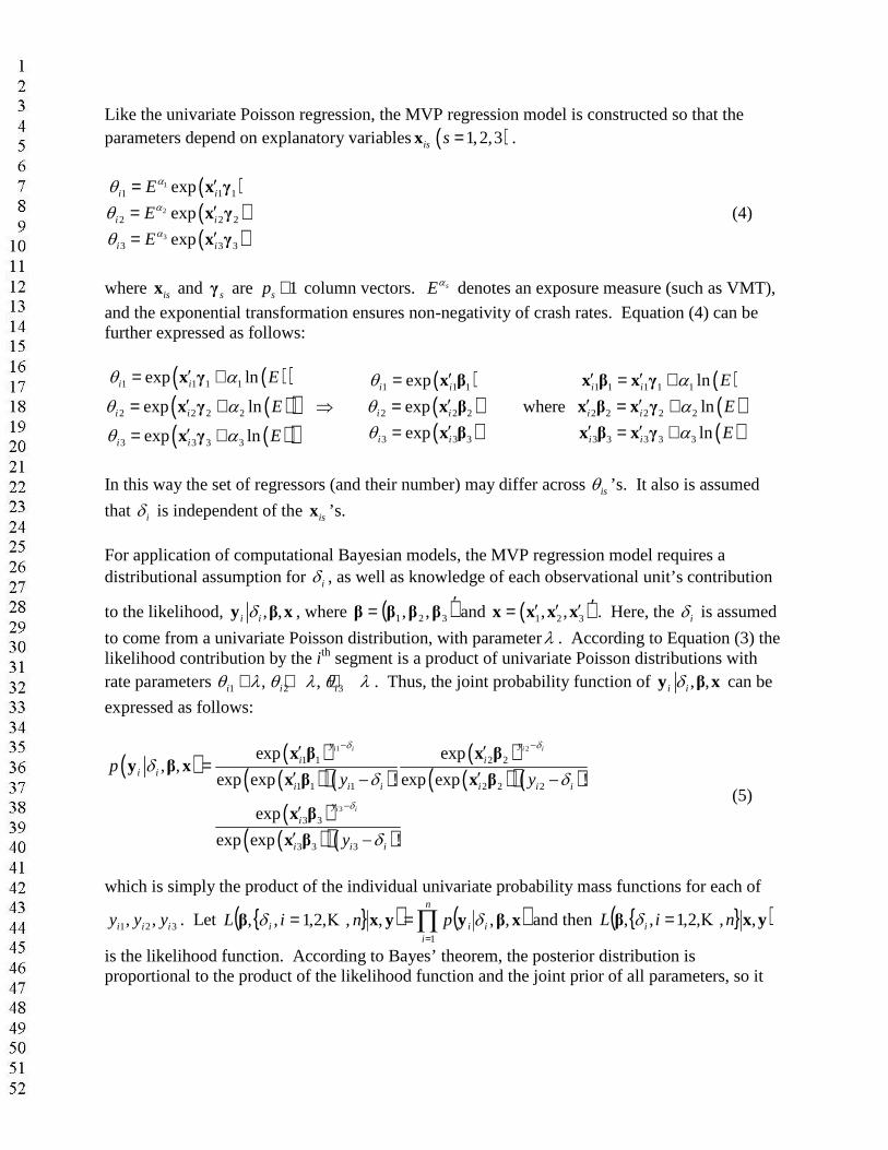
Like the univariate Poisson regression, the MVP regression model is constructed so that the parameters depend on explanatory variables isx ( )1,2,3s = .

( )( )( )

1

2

3

1 1 1

2 2 2

3 3 3

exp

exp

exp

i i

i i

i i

E

E

E

α

α

α

θθθ

′=′=′=

x γx γx γ

(4)

where isx and sγ are 1sp × column vectors. sEα denotes an exposure measure (such as VMT),

and the exponential transformation ensures non-negativity of crash rates. Equation (4) can be further expressed as follows:

( )( )( )( )( )( )

1 1 1 1

2 2 2 2

3 3 3 3

exp ln

exp ln

exp ln

i i

i i

i i

E

E

E

θ α

θ α

θ α

′= +

′= +

′= +

x γ

x γ

x γ

⇒( )( )( )

1 1 1

2 2 2

3 3 3

exp

exp

exp

i i

i i

i i

θθθ

′=′=′=

x βx βx β

where

( )( )( )

1 1 1 1 1

2 2 2 2 2

3 3 3 3 3

ln

ln

ln

i i

i i

i i

E

E

E

ααα

′ ′= +′ ′= +′ ′= +

x β x γx β x γx β x γ

In this way the set of regressors (and their number) may differ across isθ ’s. It also is assumed

that iδ is independent of the isx ’s.

For application of computational Bayesian models, the MVP regression model requires a distributional assumption for iδ , as well as knowledge of each observational unit’s contribution

to the likelihood, , ,i iδy β x , where ( )′= 321 ,, ββββ and ( )1 2 3, , ′′ ′ ′=x x x x . Here, the iδ is assumed

to come from a univariate Poisson distribution, with parameterλ . According to Equation (3) the likelihood contribution by the ith segment is a product of univariate Poisson distributions with rate parameters 1 2 3, , i i iθ λ θ λ θ λ+ + + . Thus, the joint probability function of , ,i iδy β x can be

expressed as follows:

( ) ( )( )( )( )

( )( )( )( )

( )( )( )( )

1 2

3

1 1 2 2

1 1 1 2 2 2

3 3

3 3 3

exp exp, ,

exp exp ! exp exp !

exp

exp exp !

i i i i

i i

y y

i ii i

i i i i i i

y

i

i i i

py y

y

δ δ

δ

δδ δ

δ

− −

−

′ ′=

′ ′− −

′′ −

x β x βy β x

x β x β

x βx β

(5)

which is simply the product of the individual univariate probability mass functions for each of

1 2 3, ,i i iy y y . Let { }( ) ( )∏=

==n

iiii pniL

1

,,,,,2,1,, xβyyxβ δδ Κ and then { }( )yxβ ,,,2,1,, niL i Κ=δ

is the likelihood function. According to Bayes’ theorem, the posterior distribution is proportional to the product of the likelihood function and the joint prior of all parameters, so it

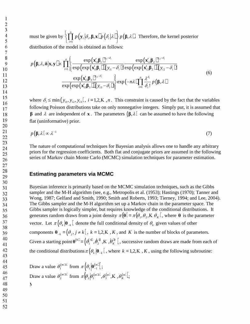
must be given by ( ) ( ) ( )1

, , ,n

i i ii

p p pδ δ λ λ=

∏ y β x β . Therefore, the kernel posterior

distribution of the model is obtained as follows:

( ) ( )( )( )( )

( )( )( )( )

( )( )( )( ) ( ) ( )

1 2

3

1 1 2 2

1 1 1 1 2 2 2

3 3

13 3 3

exp exp, , ,

exp exp ! exp exp !

exp exp ,

!exp exp !

i i i i

i i i

y yni i

i i i i i i i

y ni

i ii i i

py y

n py

δ δ

δ δ

λδ δ

λλ λδδ

− −

=

−

=

′ ′∝ ′ ′− −′ −′ −

∏

∏

x β x ββ δ x y

x β x β

x ββ

x β

(6)

where ( )1 2 3min , ,i i i iy y yδ ≤ , ni ,,2,1 Κ= . This constraint is caused by the fact that the variables

following Poisson distributions take on only nonnegative integers. Simply put, it is assumed that β and λ are independent of x . The parameters ( ),λβ can be assumed to have the following

flat (uninformative) prior.

( ) 1,p λ λ−∝β (7)

The nature of computational techniques for Bayesian analysis allows one to handle any arbitrary priors for the regression coefficients. Both flat and conjugate priors are assumed in the following series of Markov chain Monte Carlo (MCMC) simulation techniques for parameter estimation.

Estimating parameters via MCMC

Bayesian inference is primarily based on the MCMC simulation techniques, such as the Gibbs sampler and the M-H algorithm (see, e.g., Metropolis et al. (1953); Hastings (1970); Tanner andWong, 1987; Gelfand and Smith, 1990; Smith and Roberts, 1993; Tierney, 1994; and Lee, 2004). The Gibbs sampler and the M-H algorithm set up a Markov chain in the parameter space. The Gibbs sampler is logically simpler, but requires knowledge of the conditional distributions. Itgenerates random draws from a joint density ( ) ( )Kθθθππ Κ,, 21=θ , where θ is the parameter

vector. Let ( )k kπ θ −θ denote the full conditional density of kθ given values of other

components ( ),k j j kθ− = ≠θ , Kk ,,2,1 Κ= , and K is the number of blocks of parameters.

Given a starting point ( ) ( ) ( ) ( )( )0 0 0 01 2, , , Kθ θ θ=θ K , successive random draws are made from each of

the conditional distributions ( )k kπ θ −θ , where Kk ,,2,1 Κ= , using the following subroutine:

Draw a value ( )11

mθ + from ( )( )1 1mπ θ −θ ;

Draw a value ( )12

mθ + from ( ) ( ) ( )( )mK

mm θθθθπ ,,, 31

12 Κ+ ;

Μ

Draw a value ( )1mKθ

+ from ( )( )1mK Kπ θ +

−θ .

where Mm ,,2,1 Κ= . Iterating the subroutine M times produces M draws from the joint

density ( )π θ . Thus the problem of sampling a multivariate distribution is reduced to the much

easier problem of sampling from a series of univariate distributions. Under mild regularity conditions (Roberts and Smith, 1994), the sample ( ){ }Mmm ,,2,1; Κ=θ converges in distribution

to ( )π θ . In practice, one is often interested in the marginal distributions of parameters of interest.

The Gibbs sampler and M-H algorithms are the best devices for exploring such distributions.

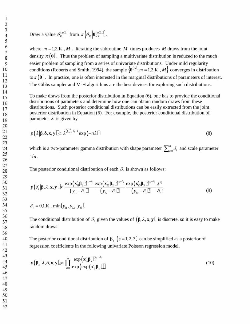
To make draws from the posterior distribution in Equation (6), one has to provide the conditional distributions of parameters and determine how one can obtain random draws from these distributions. Such posterior conditional distributions can be easily extracted from the joint posterior distribution in Equation (6). For example, the posterior conditional distribution of parameter λ is given by

( ) ( )11

, , , expn

iip nδλ λ λ=−∑∝ −β δ x y (8)

which is a two-parameter gamma distribution with shape parameter 1

n

iiδ

=∑ and scale parameter

1 n .

The posterior conditional distribution of each iδ is shown as follows:

( ) ( )( )

( )( )

( )( )

1 2 3

1 1 2 2 3 3

1 2 3

exp exp exp, , ,

! ! ! !

i i i i i i iy y y

i i ii

i i i i i i i

py y y

δ δ δ δλδ λδ δ δ δ

− − −′ ′ ′∝

− − −x β x β x β

β x y(9)

( )321 ,,min,,1,0 iiii yyyΚ=δ

The conditional distribution of iδ given the values of ( ), , ,λβ x y is discrete, so it is easy to make

random draws.

The posterior conditional distribution of sβ ( )1,2,3s = can be simplified as a posterior of

regression coefficients in the following univariate Poisson regression model.

( ) ( )( )( )1

exp, , ,

exp exp

is iynis s

si is s

pδ

λ−

=

′∝

′∏x β

β δ x yx β

(10)

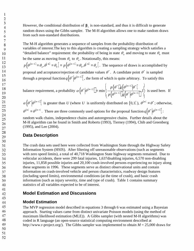
However, the conditional distribution of sβ is non-standard, and thus it is difficult to generate

random draws using the Gibbs sampler. The M-H algorithm allows one to make random draws from such non-standard distributions.

The M-H algorithm generates a sequence of samples from the probability distribution of variables of interest.The key to this algorithm is creating a sampling strategy which satisfies a “detailed balance” requirement: the probability of being in state aθ and moving to state bθ must

be the same as moving from bθ to aθ . Notationally, this means:( ) ( )( ) ( ) ( )( )1 1, ,m m m m

a b b ap pθ θ θ θ θ θ θ θ− −= = = = = . The sequence of draws is accomplished by

proposal and acceptance/rejection of candidate values *θ . A candidate point *θ is sampled

through a proposal function ( )( )1* mq θ θ − , the form of which is quite arbitrary. To satisfy this

balance requirement, a probability ( )( ) ( ) ( )( )( )( ) ( )( )

1* *

1*

1 1*min ,1

m

m

m m

p q

p q

θ θ θα θ θ

θ θ θ

−

−

− −

=

is used here. If

( )( )1* mα θ θ − is greater than U (where U is uniformly distributed on ( )0,1 ), ( ) *mθ θ= ; otherwise,

( ) ( )1m mθ θ −= . There are three commonly used options for the proposal function ( )( )1* mq θ θ − :

random walk chains, independence chains and autoregressive chains. Further details about the M-H algorithm can be found in Smith and Roberts (1993), Tierney (1994), Chib and Greenberg (1995), and Lee (2004).

Data Description

The crash data sets used here were collected from Washington State through the Highway Safety Information System (HSIS). After filtering off unreasonable observations (such as segments with zero speed limits), a total of 40,718 Washington State highway segments remained. Due to vehicular accidents, there were 299 fatal injuries, 1,637disabling injuries, 6,570 non-disabling injuries, 11,858 possible injuries and 20,100 crash-involved persons experiencing no injury along these segments in 1996. These segments serve as distinct observational units and contain information on crash-involved vehicle and person characteristics, roadway design features (including speed limits), environmental conditions (at the time of crash), and basic crashinformation (such as injury severity, time and type of crash). Table 1 contains summary statistics of all variables expected to be of interest.

Model Estimation and Discussions

Model EstimationThe MVP regression model described in equations 3 through 6 was estimated using a Bayesian approach. Starting values came from distinct univariate Poisson models (using the method ofmaximum likelihood estimation (MLE)). A Gibbs sampler (with nested M-H algorithms) wascoded in R language (an open-source statistical computing environment described at http://www.r-project.org/). The Gibbs sampler was implemented to obtain M = 25,000 draws for

each of the 96 parameters. The initial 5,000 draws were discarded as burn-ins. To help ensure chain convergence, the Gibbs sampler was implemented using two sets of initial values, and bothconverges at the same posterior distribution of parameters. Estimation results are presented in Tables 2 through 6, along with MLE results for the univariate Poisson models.

Figures 1 and 2 illustrate the estimates of posterior distributions for these regression coefficients. Based on the posterior density of λ (shown in the right-bottom panel of Figure 2), positive correlations between crash counts at different levels of severity within the segment do appear toexist in a statistically significant way among counts of different injury levels. The univariate models are a special case of the MVP, with λ equal to zero, so the MVP predictions should prove better. Calculation of average likelihood values for the estimated models versus constant-only cases provide likelihood ratio indices (LRIs) as a measure of goodness of fit. These are 0.323 for the suite of univariate models and 0.766 for the MVP approach, suggesting that the latter is superior. Both approaches predict total counts (by severity) across all roadway segments with almost no error.

Interpretation of ResultsIn addition to producing a substantially higher LRI and better estimates of total crash-involved persons (or “total injuries”), the MVP model’s estimation results offer more intuitive interpretations. For example, fatal injury rates (per VMT) rise with speed limit in the MVP models. This potentially key variable was not found to be statistically significant in the univariate model for fatal crash counts. However, the MVP model’s Bayesian results suggest far fewer statistically significant control variables.

The following discussion of results emphasizes fatal and disabling injuries (Tables 2 and 3), since these arguably are of greatest concern to agencies and policymakers. Moreover, the data on such outcomes are more likely to be reported and more reliably recorded than that for other crash outcomes. Tables 4 through 6 provide person-count model estimates for the other three severity levels. The signs of most coefficients are consistent throughout the models, indicating robust directions of effect for almost all control variables, at least in the case of severe injury (fatal and debilitating).

Parameter estimates shown in Tables 2 and 3 suggest that roadway design plays an important role in injury counts. For example, holding all other factors fixed, more fatal injuries are expected on sharper horizontal curves, while wider shoulders tend to reduce rates of both fatal and disabling injuries. Based on an average road segment’s attributes and the MVP model’s average parameter estimates, Table 7 provides estimates of percentage changes in crash frequencies as a function of various design details. For example, a 10 ft increase in shoulder width (from 10’ to 20’) is predicted to result in 18% and 23% fewer fatal and disabling injury cases per 100 million VMT, respectively. Added lanes are predicted to reduce disabling injuriesby 11%; an added median by 8.8%. Removal of access control is predicted to increase the number of disabling injuries by 36%. Oddly, none of these three key variables was predicted to have a statistically significant impact on fatal injury counts (in the MVP model). Perhaps fatal crash counts are so rare on short homogeneous roadway segments that they cannot be clearly linked to many design attributes. Nevertheless, disabling injuries may serve as a valuable proxy

for fatal crash relationships. And the MVP model offers several statistically (and practically) significant insights into these injury counts’ dependence on roadway design attributes.

Example Application: A Cost-Benefit Analysis of Raised Speed Limits

Results in Tables 2 through 7 offer several suggestions for design changes that transportation agencies might consider. As indicated in Table 7, a speed limit increase 10 mi/h (from 55 mi/h to 65 mi/h, on the “average” roadway section in the database) is predicted to increase fatal and disabling injury rates by 0.95% and 11.13%, respectively (according to the MVP model’s average parameter values). One might argue that travel time savings due to a raise in limits can offset the costs of increases in these and other crash outcomes. This section considers this question, as an example application of the model results.

Table 8 presents estimates of injury costs. Its first two rows summarize a National Highway Traffic Safety Administration (NHTSA) study by Blincoe et al. (2002). The first row presents the “market costs” of injuries (based on medical treatment, emergency services, losses in market and household productivity, insurance administration, workplace cost, and legal costs). The second row gives comprehensive costs incorporating Quality-Adjusted Life Years (QALYs), andaccounts for pain and suffering by family members. Since the HSIS database recognizes fiveinjury levels (rather than 6), injury costs were calculated using a weighted average of the six MAIS (Maximum Abbreviated Injury Scale)1 costs.

Table 9 presents driving speed increases that have been observed in a variety of published studies following speed limit increases2. Based on Table 9, there is approximately a 3.1 mi/h increase in average, observed traffic speeds if speed limits are raised 10 mph. Thus, the time savings per 100 million VMT due to a 10 mph increase in speed limits is estimated to be 106,879hours. This time savings is equivalent to $1,450,687, assuming a $15.04/vehicle-hour value of travel time savings (US DOT, 1997 and 2003). A 10 mph increase in speed limits is predicted to result in 0.029 and 1.9 more fatal and disabling injuries, respectively, and in 4.87, 13.96, and 17.16 fewer non-disabling, possible and no injury outcomes (per 100 million VMT), respectively. The equivalent average cost estimate for such shifts in injury types is estimated to be $3.34 million (in 2000 dollars, using the values of crash costs in the last row of Table 83). Therefore, the estimated cost-benefit ratio is 2.3:1. These results suggest that raising speed limits does notoffer adequate time savings benefits. However, if actual travel speeds were to increase one-to-one with speed limits (i.e., by 10 mi/h, rather than 3.1 mi/h), this ratio would change to 0.71:1. Thus, the result very much depends on how much speeds change following a speed limit change.

ConclusionsThis study developed a model that allows researchers to simultaneously model crash outcomesby severity based on a type of MVP specification that can be estimated within a Bayesian framework using Gibbs sampling. Crash counts for over 40,000 homogeneous segments ofWashington State highways in 1996 were used to estimate the model. As expected, positive correlation in unobserved factors affecting count outcomes was found to exist across severity levels, resulting in a statistically significant additive latent term.

Thanks to MCMC simulation techniques, the marginal posterior distributions of all parameters of interest were obtained, and estimation results from the MVP approach offered more intuitive interpretations and better predictions than those from the univariate Poisson models. As anticipated, the results lend themselves to several recommendations for highway safety treatments and design policies. For example, access control and wide shoulders are key for reducing severe injury, as are medians and added lanes. Moreover, using a cost-benefit approach and assumptions about travel speed changes, model results suggest that time savings from raising speed limits 10 mi/h (from 55 to 65 mi/h) may not be worth the added crash cost.

There are several enhancements that can be made in this work. The model specification relied on a one-way covariance structure, and assumed the presence of an added constant across all count types. This implies that the covariances are non-negative and identical within the segment, and that within-segment covariances are the same across segments. A more general covariance structure would allow for different correlations across all pairs of count outcomes, and a multiplicative approach may better reflect the distinctions in count magnitudes (across severities). Other forms of overdispersion and correlation also should be explored, including the mixed multinomial-Poisson model (Terza and Wilson, 1990), the multivariate negative binomial model (as employed by Kockelman [2001] and others, and currently under investigation by the authors). The use of panel data would allow one to distinguish sources of heterogeneity. And acquisition of other potentially valuable variables (such as distances to the nearest hospital and clear zone width) would also be helpful. Nevertheless, a Bayesian approach appears to offer great potential for new and different model specifications, offering richer sets of results and better predictive power. Such approaches may be critical in an area as important to human health and welfare as highway safety, even in the presence of large data sets (where classical approaches also tend to perform reasonably).

AcknowledgementsThe authors thank the Texas Department of Transportation (TxDOT) for funding this research under contract number 0-4965. The authors also are grateful to the FHWA’s Yusuf Mohamedshah for provision of the crash data sets, Drs. Shaw-Pin Miaou and Paul Damien for offering useful discussions related to methods of analysis, and Ms. Annette Perrone for editorial assistance.

Endnotes

1 MAIS denotes the highest (maximum) abbreviated injury severity score (AIS) that corresponds to a crash victim’s incurred injuries. It can take on values from 0 (minor injuries) to 5 (fatal injury).2 Most of the studies listed here (except that in NCHRP Project 17-23) examined speeds on rural interstate highways, following a change from 55 mi/h to 65 mi/h. The NCHRP (2005) study examined an urban an rural site, both with 5 mi/h increase. (The resulting average speed change was therefore doubled in that case, to estimate the change that would have occurred has the speed limit change been 10 mi/h.)3 Mrozek and Taylor (2002) investigated the value of a statistical life (VOSL) using a meta-analysis. Based on 33 previous studies, they recommended a VOSL of $1.5 to $2.5 million, which is considerably lower than NHTSA’s $3.37 million recommendation. However, the average VOSL of the 33 studies is about $5.59 million. If this $5.59 million value (per life) were used here and other injury costs were inflated by a ratio of 1.66 (=5.59 million/3.37 million), the cost-benefit ratio would become 1:2.21, suggesting that speed limits could offer some valuable time savings benefits.

ReferencesAbdel-Aty, M.A., and Radwan, A.E. (2000). Modeling traffic accident occurrence and

involvement. Accident Analysis and Prevention, 32(5), 633-642.Balkin, S., and Ord, J.K. (2001). Assessing the impact of speed-limit increases on fatal interstate

crashes. Journal of Transportation and Statistics, 4(1), 1-26.Bijleveld, F.D. (2005). The covariance between the number of accidents and the number of

victims in multivariate analysis of accident related outcomes. Accident Analysis and Prevention, 37(4), 591-600.

Blincoe, L., Seay, A., Zaloshnja, E., Miller, T., Romano, E., Luchter, S., and Spicer R. (2002).The Economic Impact of Motor Vehicle Crashes, 2000. Retrieved May 31, 2005, from http://www.nhtsa.dot.gov/staticfiles/DOT/NHTSA/Communication and ConsumerInformation/Articles/Associated Files/EconomicImpact2000.pdf.

Brown, D. B., Maghsoodloo, S., and Ardle, M. E. (1990) The Safety Impact of 65 MPH Speed Limit: A Case Study Using Alabama Accident Records. Journal of Safety Research, 21(4), 125-139.

Chib, S., and Greenberg, E. (1995). Understanding the Metropolis-Hastings algorithm. The American Statistician, 49(4), 327-335.

Chin, H.C.C., and Quddus, M.A. (2003). Applying the random effect negative binomial model to examine traffic accident occurrence at signalized intersections. Accident Analysis and Prevention, 35(2), 253-259.

Christiansen, C.L., Morris, C.N., and Pendleton, O.J. (1992). A Hierarchical Poisson Model with Beta Adjustments for Traffic Accident Analysis (Technical Report 103). Austin, TX: Center for Statistical Sciences, The University of Texas at Austin.

Freedman, M., Esterlitz, J. R. (1990) Effect of the 65 mph Speed Limit on Speeds in Three States, Transportation Research Record, No.1281, 52-61.

Fridstrøm, L., Ifver, J., Ingebrigtsen, S., Kulmala, R., and Thomsen, L.K. (1995). Measuring the contribution of randomness, exposure, weather, and daylight to the various in road accident counts. Accident Analysis and Prevention, 27(1), 1-20.

Garber, N.J., and Wu, L. (2001). Stochastic Models Relating Crash Probabilities with Geometric and Corresponding Traffic Characteristics Data (UVACTS-5-15-74). Charlottesville, VA: Center for Transportation Studies, University of Virginia.

Gelfand, A.E., and Smith, F.M. (1990), Sampling-based approaches to calculating marginal densities. Journal of the American Statistical Association, 85(410), 398-409.

Hastings, W.K. (1970). Monte Carlo sampling methods using Markov chains and their applications. Biometrika, 57(1), 97-109.

Hauer, E. (1986). On the estimation of the expected number of accidents. Accident Analysis and Prevention, 18(1), 1-12.

Hauer, E. (1997). Observational Before-After Studies in Road Safety. Pergamon, Oxford.Hauer, E. (2001). Overdispersion in modeling accidents on road sections and in empirical bayes

estimation. Accident Analysis and Prevention, 33(6), 799-808.Johansson, P. (1996). Speed limitation and motorway casualties: A time-series count data

regression approach. Accident Analysis and Prevention, 28(1), 73-87.Karlis, D. (2003). An EM algorithm for multivariate Poisson distribution and related models.

Journal of Applied Statistics, 30(1), 63-77.

Kockelman, K. (2001). A Model for Time- and Budget-Constrained Activity Demand Analysis. Transportation Research 35B (3): 255-269.

Kumara, S.P., and Chin, H.C. (2003). Modeling accident occurrence at signalized T intersections with special emphasis on excess zeros. Traffic Injury Prevention, 4(1), 53-57.

Kweon, Y.J., and Kockelman, K. (2005). The safety effects of speed limit changes: use of panel models, including speed, use, and design variables. Proceedings of Transportation Research Board Annual Meeting, Washington D.C. (January 2005), and forthcoming in Transportation Research Record.Lee, J., and Mannering, F.L. (2002). Impact of roadside features on the frequency and severity of run-off-roadway accidents: An empirical analysis. Accident Analysis and Prevention, 34(2), 149-161.

Lee, P.M. (2004). Bayesian Statistics: An Introduction. New York, NY: Oxford University Press Inc.

Li, C.C., Lu, J.C., Park, J., Kim, K., Brinkley, P.A. & Peterson, J.P. (1999). Multivariate zero-inflated Poisson models and their applications. Technometrics, 41(1), 29-38.

Lord, D., Persaud, B.N. (2000). Accident prediction models with and without trend: application of the generalized estimating equations procedure. Transportation Research Record 1717, 102-108.

Lord, D., Washington, S.P., and Ivan, J.N. (2005). Poisson, Poisson-gamma and zero-inflated regression models of motor vehicle crashes: balancing statistical fit and theory. Accident Analysis and Prevention, 37(1), 35-46.

Mace, D. J., and R. Heckard (1991) Effect of the 65 mph Speed Limit on Travel Speeds and Related Crashes. Report No. DOT HS 807 764, National Highway Traffic Safety Administration, Washington, DC.

MacNab, Y.C. (2003). A Bayesian hierarchical model for accident and injury surveillance. Accident Analysis and Prevention, 35(1), 91-102.

Metropolis, N., Rosenbluth, A.W., Rosenbluth, M.N., Teller, A.H., and Teller, E. (1953). Equation of state calculations by fast computing machines. The Journal of Chemical Physics, 21(6), 1087-1092.

Miaou, S.P., Hu, P.S., Wright, T., Davis, S.C., and Rathi, A.K. (1993). Development of Relationship Between Truck Accidents and Geometric Design: Phase I (FHWA-RD-91-124). Oak Ridge, TN: Oak Ridge National Laboratory.

Miaou, S.P., and Lum, H. (1993). Modeling vehicle accidents and highway geometric design relationships. Accident Analysis and Prevention, 25(6), 689-709.

Miaou, S.P. (1994). The relationship between truck accidents and geometric design of road sections: Poisson versus negative binomial regressions. Accident Analysis and Prevention, 26(4), 471-482.

Miaou, S.P. (1996). Measuring the Goodness-of-fit of Accident Prediction Models (FHWA-RD-96-040). Oak Ridge, TN: Oak Ridge National Laboratory.

Miaou, S.P. (2001). Estimating Roadside Encroachment Rates with the Combined Strengths of Accident- and Encroachment-Based Approaches (FHWA-RD-01-124). Oak Ridge, TN: Oak Ridge National Laboratory.

Miaou, S.P., and Lord, D. (2003). Modeling traffic crash-flow relationships for intersections: dispersion parameter, functional form, and bayes versus empirical bayes. Transportation Research Record 1840, 31-40

Miaou, S.P., and Song, J.J. (2005). Bayesian ranking of sites for engineering safety improvements: Decision parameter, treatability concept, statistical criterion, and spatial dependence. Accident Analysis and Prevention, 37(4), 699-720.

Mrozek, J.R., and Taylor, L.O. (2002) What Determines the Value of Life? A Meta-Analysis. Journal of Policy Analysis and Management, 21(2), 253-270.

NCHRP (2005) Safety Impacts and Other Implications of Raised Speed Limits on High-Speed Roads. National Cooperative Highway Research Program Project #17-23, Report Draft, Kockelman, K and Bottom, J. Transportation Research Board. Washington, D.C.

NHTSA (1989) Report to Congress on the Effects of the 65 mph Speed Limit During 1987. Washington, DC: U.S. Department of Transportation.

NHTSA (1992) Report to Congress on the Effects of the 65 mph Speed Limit Through 1990. Washington, DC: U.S. Department of Transportation.

NHTSA (2005) Traffic Safety Fact: Research Notes. National Highway Traffic Safety Administration, Report* DOT HS 809 831. January. Washington, D.C.

Noland, R.B., and Quddus, M.A. (2004). A spatially disaggregate analysis of road casualties in England. Accident Analysis and Prevention, 36(6), 973-984

Parker, M. R. (1997) Effects of Raising and Lowering Speed Limits on Selected Roadway Sections. Report No. FHWA-RD-92-084, Federal Highway Administration, Washington, DC.

Pernia, J., Lu, J.J., and Peng, H. (2004). Safety Issues Related to Two-way Left-turn Lanes (Final Technical Report). Tampa, FL: Department of Civil and Environmental Engineering, University of South Florida.

Pfefer, F. M., Stenzel, W. W., and Lee, B. D. (1991) Safety Impact of the 65-mph Speed Limit: A Time Series Analysis. Transportation Research Record, No. 1318, 22-33.

Qin, X., Ivan, J.N., and Ravishanker, N. (2004). Selecting exposure measures in crash rate prediction for two-lane highway segments. Accident Analysis and Prevention, 36(2), 183-191.

Roberts, G.O., and Smith, F.M. (1994). Simple conditions for the convergence of the Gibbs sampler and Metropolis-Hastings algorithms. Stochastic Processes and their Applications, 49(2), 207-216.

Rodriguez, D.A., Rocha, M., Khattak, A.J., and Belzer, M.H. (2003). Effects of truck driver wages and working conditions on highway safety: Case study. Transportation Research Record 1833, 95-102.

Schrank, D., and Lomax, T. (2002). The 2002 Urban Mobility Report. Texas Transportation Institute, The Texas AandM University System.

Shankar, V., Milton, J., and Mannering, F.L. (1997). Modeling accident frequency as zero-altered probability processes: an empirical inquiry. Accident Analysis and Prevention, 29(6), 829-837.

Shankar V.N., Ulfarsson, G.F., Pendyala, R.M., and Nebergall, M.B. (2003). Modeling crashes involving pedestrians and motorized traffic. Safety Science, 41(7), 557-640.

Smith, A.F.M., and Roberts, G.O. (1993). Bayesian computation via the Gibbs sampler and related Markov chain Monte Carlo methods. Journal of the Royal Statistical Society, Series B, 55(1), 3-23.

Tanner, M.A., and Wong, W.H. (1987). The calculation of posterior distribution by data augmentation. Journal of the American Statistical Association, 82(398), 520-540.

Terza, J.V., and Wilson, P. (1990). Analyzing frequencies of several types of events: a mixed multinomial-Poisson approach. The Review of Economics and Statistics, 72(10), 108-115.

Tierney, L. (1994). Markov chains for exploring posterior distributions. The Annals of Statistics, 22(4), 1701-1728.

TRB. (1998) Managing Speed – Review of Current Practice for Setting and Enforcing Speed Limits. TRB Special Report 254, National Academy Press, Washington, D.C.

Tsionas E.G. (2001). Bayesian multivariate Poisson regression. Communications in Statistics –Theory and Methods, 30(2), 243-255.

Ulfarsson, G.F., and Shankar, V.N. (2003). Accident count model based on multiyear cross-sectional roadway data with serial correlation. Transportation Research Record 1840, 193-197.

U.S. Department of Transportation. (1997) Departmental Guidance for the Valuation of Travel Time in Economic Analysis. Office of the Secretary of Transportation, U.S. Department of Transportation, 1997. Available at: http://ostpxweb.dot.gov/policy/Data/VOT97guid.pdf

U.S. Department of Transportation. (2003) Revised Departmental Guidance: Valuation of Travel Time in Economic Analysis. Office of the Secretary of Transportation, U.S. Department of Transportation. Available at: http://ostpxweb.dot.gov/policy/Data/VOTrevision1_2-11-03.pdf.

Vogt, A., and Bared, J.G. (1998). Accident Models for Two-lane Rural Roads: Segments and Intersections (FHWA-RD-98-133). McLean, VA: Turner Fairbank Highway Research Center, Federal Highway Administration.

Vogt, A. (1999). Crash Models for Rural Intersections: Four-lane by Two-lane Stop-controlled and Two-lane by Two-lane Signalized (FHWA-RD-99-128). McLean, VA: Turner Fairbank Highway Research Center, Federal Highway Administration.

Zegeer, C.V., Stewart, J.R., Huang, H.H., and Lagerwey, P.A. (2002). Safety Effects of Marked Vs. Unmarked Crosswalks at Uncontrolled Locations: Executive Summary and Recommended Guidelines (FHWA-RD-01-075). Chapel Hill, NC: Highway Safety Research Center, University of North Carolina.

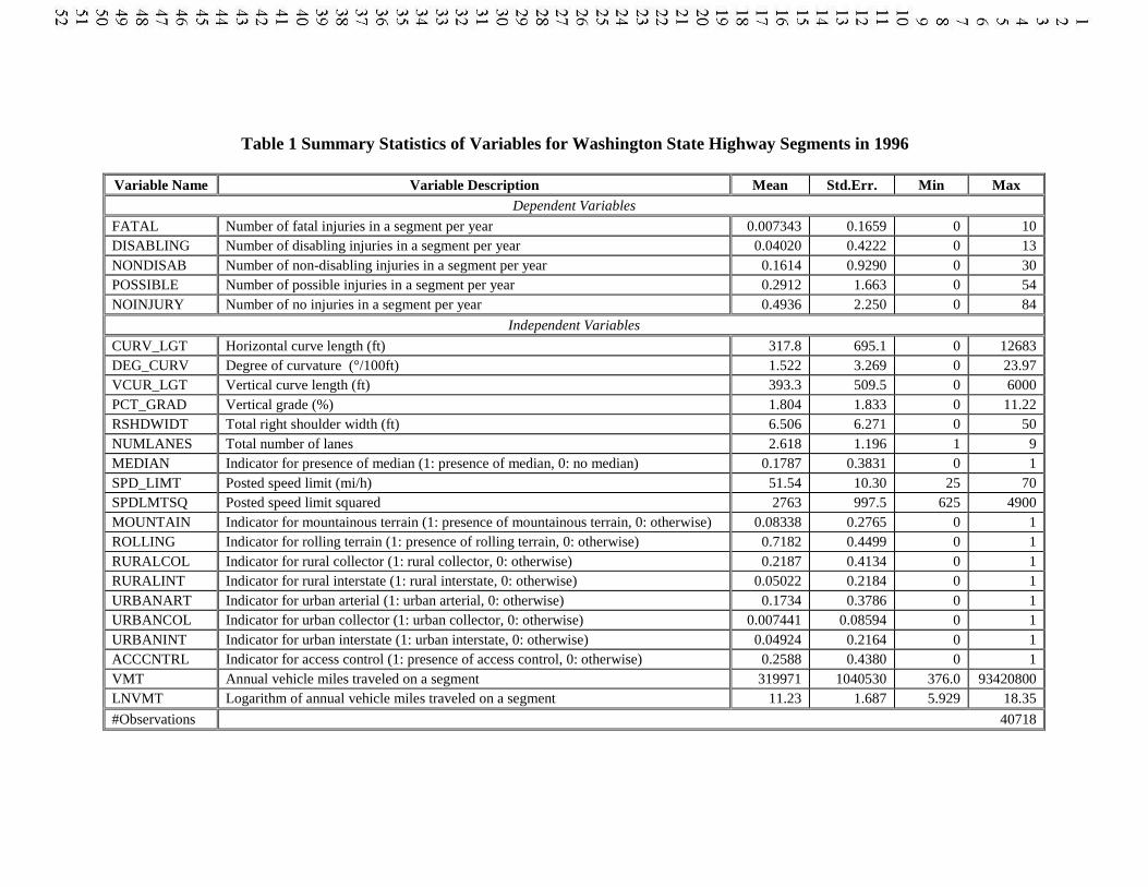
Table 1 Summary Statistics of Variables for Washington State Highway Segments in 1996

Variable Name Variable Description Mean Std.Err. Min MaxDependent Variables

FATAL Number of fatal injuries in a segment per year 0.007343 0.1659 0 10DISABLING Number of disabling injuries in a segment per year 0.04020 0.4222 0 13NONDISAB Number of non-disabling injuries in a segment per year 0.1614 0.9290 0 30POSSIBLE Number of possible injuries in a segment per year 0.2912 1.663 0 54NOINJURY Number of no injuries in a segment per year 0.4936 2.250 0 84

Independent Variables

CURV_LGT Horizontal curve length (ft) 317.8 695.1 0 12683DEG_CURV Degree of curvature (°/100ft) 1.522 3.269 0 23.97VCUR_LGT Vertical curve length (ft) 393.3 509.5 0 6000PCT_GRAD Vertical grade (%) 1.804 1.833 0 11.22RSHDWIDT Total right shoulder width (ft) 6.506 6.271 0 50NUMLANES Total number of lanes 2.618 1.196 1 9MEDIAN Indicator for presence of median (1: presence of median, 0: no median) 0.1787 0.3831 0 1SPD_LIMT Posted speed limit (mi/h) 51.54 10.30 25 70SPDLMTSQ Posted speed limit squared 2763 997.5 625 4900MOUNTAIN Indicator for mountainous terrain (1: presence of mountainous terrain, 0: otherwise) 0.08338 0.2765 0 1ROLLING Indicator for rolling terrain (1: presence of rolling terrain, 0: otherwise) 0.7182 0.4499 0 1RURALCOL Indicator for rural collector (1: rural collector, 0: otherwise) 0.2187 0.4134 0 1RURALINT Indicator for rural interstate (1: rural interstate, 0: otherwise) 0.05022 0.2184 0 1URBANART Indicator for urban arterial (1: urban arterial, 0: otherwise) 0.1734 0.3786 0 1URBANCOL Indicator for urban collector (1: urban collector, 0: otherwise) 0.007441 0.08594 0 1URBANINT Indicator for urban interstate (1: urban interstate, 0: otherwise) 0.04924 0.2164 0 1ACCCNTRL Indicator for access control (1: presence of access control, 0: otherwise) 0.2588 0.4380 0 1VMT Annual vehicle miles traveled on a segment 319971 1040530 376.0 93420800LNVMT Logarithm of annual vehicle miles traveled on a segment 11.23 1.687 5.929 18.35

#Observations 40718

Table 2 Fatal Injury Frequency Models for Washington State Crash Data 1996

Univariate Poisson Regression(MLE)

Multivariate Poisson Regression(Gibbs Sampler)

Coef. Std. Err. P-value Mean Std. Err. The 95% (2.5-97.5%) HDR

Constant -13.14 0.7778 0.000 -12.92* 1.433 -15.71 -10.10

CURV_LGT 1.894E-04 4.997E-05 0.000 -6.639E-05 9.423E-05 -2.522E-04 1.160E-04

DEG_CURV 0.01212* 0.006019 0.0003532 0.02395

VCUR_LGT -1.909E-04 1.105E-04 0.084 5.526E-05 1.246E-04 -1.875E-04 3.005E-04

PCT_GRAD 0.01286 0.01927 -0.02470 0.05098

RSHDWIDT -0.01992* 0.005541 -0.03088 -0.0091049

NUMLANES -0.2130 0.07369 0.004 -0.02792 0.07470 -0.1728 0.1195

MEDIAN -0.4290 0.2475 0.083 0.08228 0.3733 -0.6455 0.8162

SPD_LIMT 0.03435 0.009882 0.001 0.01214* 0.005055 0.002259 0.02202

SPDLMTSQ -9.432E-05 1.860E-04 -4.599E-04 2.702E-04

MOUNTAIN -1.782 0.5943 0.003 1.943 2.853 -3.657 7.524

ROLLING -0.3199 0.1335 0.017 0.2211 0.3013 -0.3655 0.8197

RURALCOL -0.7587 0.3087 0.014 0.08142 0.2868 -0.4803 0.6472

RURALINT 1.157 0.2793 0.000 -0.03326 0.3041 -0.6300 0.5658

URBANART 0.6766 0.1911 0.000 0.9335 1.285 -1.572 3.439

URBANCOL -29.37 32.26 -92.84 33.40

URBANINT 0.6593 0.3343 0.049 0.8876 1.168 -1.402 3.155

ACCCNTRL -0.4500 0.2025 0.026 -0.2981 0.3508 -0.9797 0.3906

LNVMT 0.6035 0.05141 0.000 0.5964* 0.1053 0.3887 0.8037

Note: An asterisk (*) signifies that parameters differ from zero in a statistically significant way, based on the 95% (2.5-97.5) high density region (HDR).

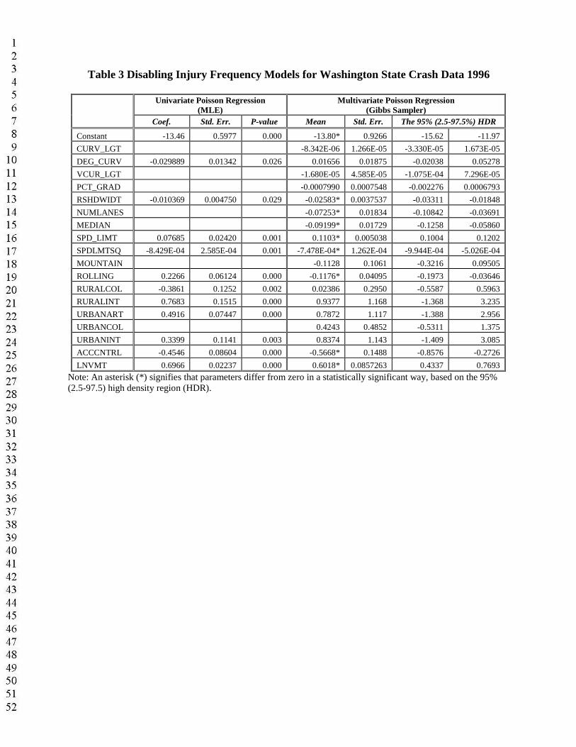
Table 3 Disabling Injury Frequency Models for Washington State Crash Data 1996




Constant -13.46 0.5977 0.000 -13.80* 0.9266 -15.62 -11.97

CURV_LGT -8.342E-06 1.266E-05 -3.330E-05 1.673E-05

DEG_CURV -0.029889 0.01342 0.026 0.01656 0.01875 -0.02038 0.05278

VCUR_LGT -1.680E-05 4.585E-05 -1.075E-04 7.296E-05

PCT_GRAD -0.0007990 0.0007548 -0.002276 0.0006793

RSHDWIDT -0.010369 0.004750 0.029 -0.02583* 0.0037537 -0.03311 -0.01848

NUMLANES -0.07253* 0.01834 -0.10842 -0.03691

MEDIAN -0.09199* 0.01729 -0.1258 -0.05860

SPD_LIMT 0.07685 0.02420 0.001 0.1103* 0.005038 0.1004 0.1202

SPDLMTSQ -8.429E-04 2.585E-04 0.001 -7.478E-04* 1.262E-04 -9.944E-04 -5.026E-04

MOUNTAIN -0.1128 0.1061 -0.3216 0.09505

ROLLING 0.2266 0.06124 0.000 -0.1176* 0.04095 -0.1973 -0.03646

RURALCOL -0.3861 0.1252 0.002 0.02386 0.2950 -0.5587 0.5963

RURALINT 0.7683 0.1515 0.000 0.9377 1.168 -1.368 3.235

URBANART 0.4916 0.07447 0.000 0.7872 1.117 -1.388 2.956

URBANCOL 0.4243 0.4852 -0.5311 1.375

URBANINT 0.3399 0.1141 0.003 0.8374 1.143 -1.409 3.085

ACCCNTRL -0.4546 0.08604 0.000 -0.5668* 0.1488 -0.8576 -0.2726

LNVMT 0.6966 0.02237 0.000 0.6018* 0.0857263 0.4337 0.7693


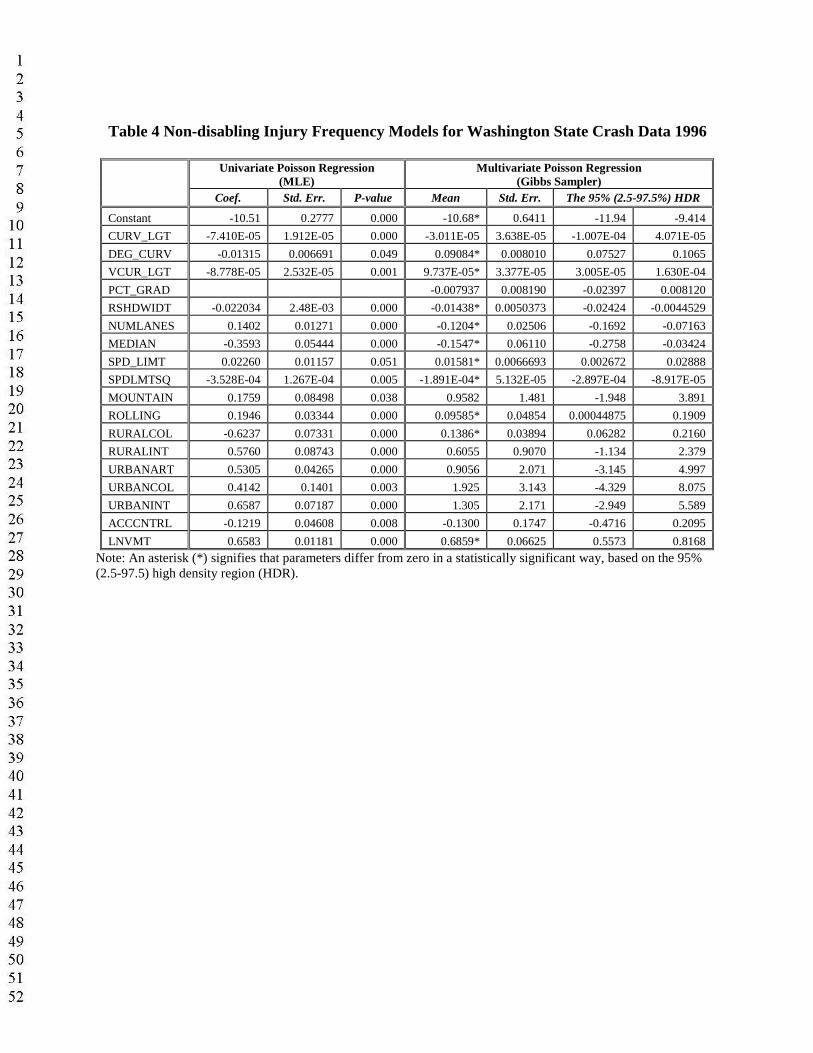
Table 4 Non-disabling Injury Frequency Models for Washington State Crash Data 1996




Constant -10.51 0.2777 0.000 -10.68* 0.6411 -11.94 -9.414

CURV_LGT -7.410E-05 1.912E-05 0.000 -3.011E-05 3.638E-05 -1.007E-04 4.071E-05

DEG_CURV -0.01315 0.006691 0.049 0.09084* 0.008010 0.07527 0.1065

VCUR_LGT -8.778E-05 2.532E-05 0.001 9.737E-05* 3.377E-05 3.005E-05 1.630E-04

PCT_GRAD -0.007937 0.008190 -0.02397 0.008120

RSHDWIDT -0.022034 2.48E-03 0.000 -0.01438* 0.0050373 -0.02424 -0.0044529

NUMLANES 0.1402 0.01271 0.000 -0.1204* 0.02506 -0.1692 -0.07163

MEDIAN -0.3593 0.05444 0.000 -0.1547* 0.06110 -0.2758 -0.03424

SPD_LIMT 0.02260 0.01157 0.051 0.01581* 0.0066693 0.002672 0.02888

SPDLMTSQ -3.528E-04 1.267E-04 0.005 -1.891E-04* 5.132E-05 -2.897E-04 -8.917E-05

MOUNTAIN 0.1759 0.08498 0.038 0.9582 1.481 -1.948 3.891

ROLLING 0.1946 0.03344 0.000 0.09585* 0.04854 0.00044875 0.1909

RURALCOL -0.6237 0.07331 0.000 0.1386* 0.03894 0.06282 0.2160

RURALINT 0.5760 0.08743 0.000 0.6055 0.9070 -1.134 2.379

URBANART 0.5305 0.04265 0.000 0.9056 2.071 -3.145 4.997

URBANCOL 0.4142 0.1401 0.003 1.925 3.143 -4.329 8.075

URBANINT 0.6587 0.07187 0.000 1.305 2.171 -2.949 5.589

ACCCNTRL -0.1219 0.04608 0.008 -0.1300 0.1747 -0.4716 0.2095

LNVMT 0.6583 0.01181 0.000 0.6859* 0.06625 0.5573 0.8168


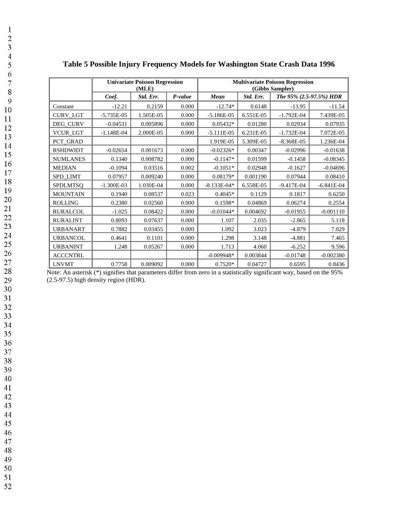
Table 5 Possible Injury Frequency Models for Washington State Crash Data 1996




Constant -12.21 0.2159 0.000 -12.74* 0.6148 -13.95 -11.54

CURV_LGT -5.735E-05 1.505E-05 0.000 -5.186E-05 6.551E-05 -1.792E-04 7.439E-05

DEG_CURV -0.04531 0.005896 0.000 0.05432* 0.01280 0.02934 0.07935

VCUR_LGT -1.148E-04 2.000E-05 0.000 -5.111E-05 6.231E-05 -1.732E-04 7.072E-05

PCT_GRAD 1.919E-05 5.309E-05 -8.368E-05 1.236E-04

RSHDWIDT -0.02654 0.001673 0.000 -0.02326* 0.00347 -0.02996 -0.01638

NUMLANES 0.1340 0.008782 0.000 -0.1147* 0.01599 -0.1458 -0.08345

MEDIAN -0.1094 0.03516 0.002 -0.1051* 0.02948 -0.1627 -0.04696

SPD_LIMT 0.07957 0.009240 0.000 0.08179* 0.001190 0.07944 0.08410

SPDLMTSQ -1.300E-03 1.030E-04 0.000 -8.133E-04* 6.558E-05 -9.417E-04 -6.841E-04

MOUNTAIN 0.1940 0.08537 0.023 0.4045* 0.1129 0.1817 0.6250

ROLLING 0.2380 0.02560 0.000 0.1598* 0.04869 0.06274 0.2554

RURALCOL -1.025 0.08422 0.000 -0.01044* 0.004692 -0.01955 -0.001110

RURALINT 0.8093 0.07637 0.000 1.107 2.035 -2.865 5.118

URBANART 0.7882 0.03455 0.000 1.092 3.023 -4.879 7.029

URBANCOL 0.4641 0.1101 0.000 1.298 3.148 -4.881 7.465

URBANINT 1.248 0.05267 0.000 1.713 4.060 -6.252 9.596

ACCCNTRL -0.009948* 0.003844 -0.01748 -0.002380

LNVMT 0.7758 0.009092 0.000 0.7520* 0.04727 0.6595 0.8436


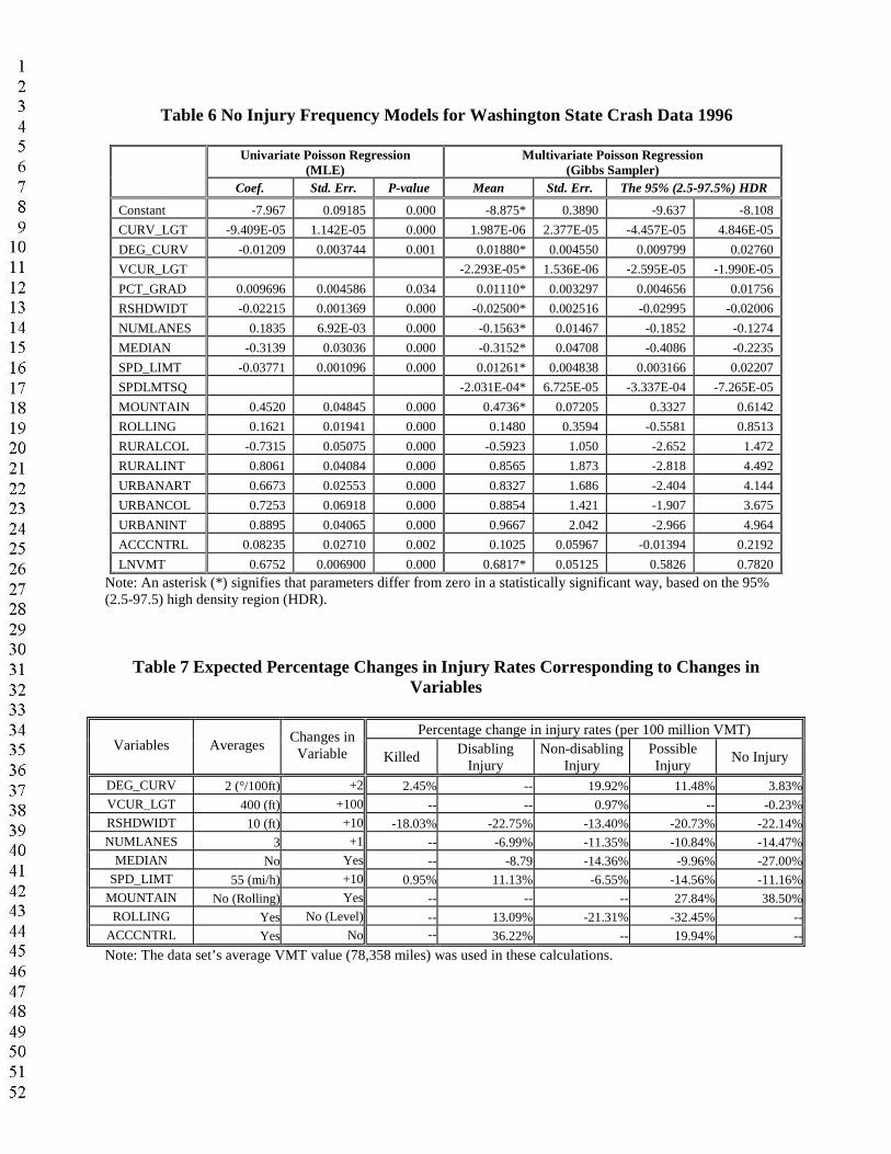
Table 6 No Injury Frequency Models for Washington State Crash Data 1996




Constant -7.967 0.09185 0.000 -8.875* 0.3890 -9.637 -8.108

CURV_LGT -9.409E-05 1.142E-05 0.000 1.987E-06 2.377E-05 -4.457E-05 4.846E-05

DEG_CURV -0.01209 0.003744 0.001 0.01880* 0.004550 0.009799 0.02760

VCUR_LGT -2.293E-05* 1.536E-06 -2.595E-05 -1.990E-05

PCT_GRAD 0.009696 0.004586 0.034 0.01110* 0.003297 0.004656 0.01756

RSHDWIDT -0.02215 0.001369 0.000 -0.02500* 0.002516 -0.02995 -0.02006

NUMLANES 0.1835 6.92E-03 0.000 -0.1563* 0.01467 -0.1852 -0.1274

MEDIAN -0.3139 0.03036 0.000 -0.3152* 0.04708 -0.4086 -0.2235

SPD_LIMT -0.03771 0.001096 0.000 0.01261* 0.004838 0.003166 0.02207

SPDLMTSQ -2.031E-04* 6.725E-05 -3.337E-04 -7.265E-05

MOUNTAIN 0.4520 0.04845 0.000 0.4736* 0.07205 0.3327 0.6142

ROLLING 0.1621 0.01941 0.000 0.1480 0.3594 -0.5581 0.8513

RURALCOL -0.7315 0.05075 0.000 -0.5923 1.050 -2.652 1.472

RURALINT 0.8061 0.04084 0.000 0.8565 1.873 -2.818 4.492

URBANART 0.6673 0.02553 0.000 0.8327 1.686 -2.404 4.144

URBANCOL 0.7253 0.06918 0.000 0.8854 1.421 -1.907 3.675

URBANINT 0.8895 0.04065 0.000 0.9667 2.042 -2.966 4.964

ACCCNTRL 0.08235 0.02710 0.002 0.1025 0.05967 -0.01394 0.2192

LNVMT 0.6752 0.006900 0.000 0.6817* 0.05125 0.5826 0.7820


Table 7 Expected Percentage Changes in Injury Rates Corresponding to Changes in Variables

Percentage change in injury rates (per 100 million VMT)Variables Averages

Changes in Variable Killed

Disabling Injury

Non-disabling Injury

Possible Injury

No Injury

DEG_CURV 2 (°/100ft) +2 2.45% -- 19.92% 11.48% 3.83%VCUR_LGT 400 (ft) +100 -- -- 0.97% -- -0.23%RSHDWIDT 10 (ft) +10 -18.03% -22.75% -13.40% -20.73% -22.14%NUMLANES 3 +1 -- -6.99% -11.35% -10.84% -14.47%

MEDIAN No Yes -- -8.79 -14.36% -9.96% -27.00%SPD_LIMT 55 (mi/h) +10 0.95% 11.13% -6.55% -14.56% -11.16%

MOUNTAIN No (Rolling) Yes -- -- -- 27.84% 38.50%ROLLING Yes No (Level) -- 13.09% -21.31% -32.45% --

ACCCNTRL Yes No -- 36.22% -- 19.94% --

Note: The data set’s average VMT value (78,358 miles) was used in these calculations.

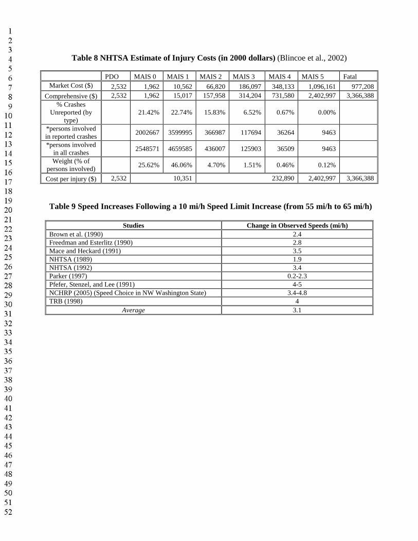
Table 8 NHTSA Estimate of Injury Costs (in 2000 dollars) (Blincoe et al., 2002)

PDO MAIS 0 MAIS 1 MAIS 2 MAIS 3 MAIS 4 MAIS 5 FatalMarket Cost ($) 2,532 1,962 10,562 66,820 186,097 348,133 1,096,161 977,208

Comprehensive ($) 2,532 1,962 15,017 157,958 314,204 731,580 2,402,997 3,366,388% Crashes

Unreported (by type)

21.42% 22.74% 15.83% 6.52% 0.67% 0.00%

*persons involved in reported crashes

2002667 3599995 366987 117694 36264 9463

*persons involved in all crashes

2548571 4659585 436007 125903 36509 9463

Weight (% of persons involved)

25.62% 46.06% 4.70% 1.51% 0.46% 0.12%

Cost per injury ($) 2,532 10,351 232,890 2,402,997 3,366,388

Table 9 Speed Increases Following a 10 mi/h Speed Limit Increase (from 55 mi/h to 65 mi/h)

Studies Change in Observed Speeds (mi/h)Brown et al. (1990) 2.4Freedman and Esterlitz (1990) 2.8Mace and Heckard (1991) 3.5NHTSA (1989) 1.9NHTSA (1992) 3.4Parker (1997) 0.2-2.3Pfefer, Stenzel, and Lee (1991) 4-5 NCHRP (2005) (Speed Choice in NW Washington State) 3.4-4.8TRB (1998) 4

Average 3.1

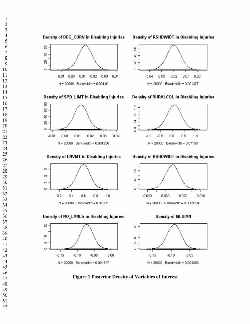
Figure 1 Posterior Density of Variables of Interest

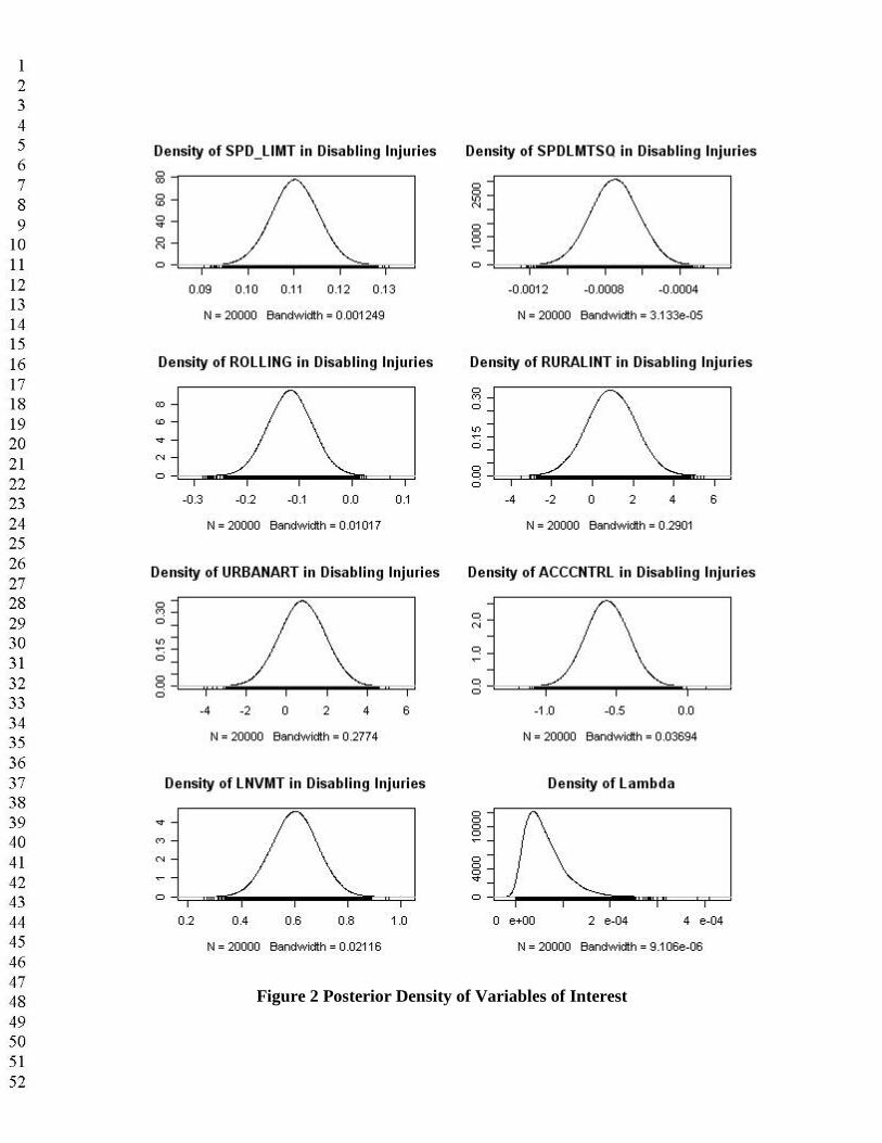
Figure 2 Posterior Density of Variables of Interest

bayesian multivariate poisson regression for models of ... · bayesian multivariate poisson...

Documents