Bayesian Learning for Hardware and SoftwareConfiguration Co-Optimization

Yi DingUniversity of Chicagodingy@uchicago.edu

Ahsan PervaizUniversity of Chicagoahsanp@uchicago.edu

Sanjay KrishnanUniversity of Chicagoskr@cs.uchicago.edu

Henry HoffmannUniversity of Chicago

hankhoffmann@cs.uchicago.edu

Abstract—Both hardware and software systems are increas-ingly configurable, which poses a challenge to finding the highestperformance configuration due to the tremendous search space.Prior scheduling and resource management work uses machinelearning (ML) to find high-performance configurations for eitherthe hardware or software configurations alone while assumingthe other is fixed. Such separate optimization is problematicbecause a software configuration that is fast on one hardwarearchitecture can be up to 50% slower on another. The maindifficulty of co-optimization is the massive search space overboth hardware and software configurations because accuratelearning models require large amounts of labeled training data,and thus long periods of data collection and configuration search.To achieve co-optimization with significantly smaller trainingsets, we present Paprika, a scheduler that simultaneously selectshardware and software configurations using a Bayesian learningapproach. Paprika augments software configuration parameterswith hardware features seamlessly and efficiently via one-hotencoding and parameter selection. To reduce the impact of thesearch space, Paprika actively queries configurations based ona novel ensemble optimization objective. The intuition of thisensemble is to combine three prior optimizers to implicitly nego-tiate the exploration–exploitation tradeoff. We evaluate Paprikawith ten Spark workloads on three hardware architectures andfind that, compared to prior work, Paprika produces runtimesthat are 12–38% closer to the optimal.

I. Introduction

Modern computing systems expose diverse configurationparameters whose interactions have surprising effects on per-formance. For hardware systems, the variety of hardwareresources constitutes the hardware configurations [7], [73]. Forsoftware systems, configuration complexity is escalating dueto the rapidly increasing number of configuration parameters.For example, the size of parameters for Hadoop MapReduceincreased by over 9 times within 8 years [65]. Numerousstudies show that managing configuration parameters is crucialto achieve high performance [60], [66].

The increase in configurability puts a great burden onsystem designers and administrators to tune parameters so thatthe combined software-hardware system operates at optimalperformance. Recent schedulers and resource managers incor-porate Machine learning (ML) to model system performanceas a function of configurations, allowing the scheduler toselect the best configuration for a given workload (see recentsurveys for a broad overview [42], [72]). Despite this success,these learning approaches have limitations to their efficacy inmodern computing environments:

• Separate optimization for hardware and softwaresystems. Prior work generally focuses on either hard-ware [18], [20], [28] or software [19], [75]. However,modern computing environments, such as datacenters, areheterogeneous, meaning that a given workload can bescheduled on different types of hardware. Yet, a softwareconfiguration that is optimal on one hardware system canwork poorly on different hardware, even for the sameworkload (see Section III-A). Therefore, it is crucial toco-optimize hardware and software configurations.

• Inefficient configuration parameter tuning. A commonapproach for parameter-tuning is running small (< 5parameter) grid searches, optimizing each parameter sep-arately [4]. However, computer systems easily scale up to> 20 parameters consisting of both hardware and softwareconfigurations (see Section V-A), rendering grid search apoor choice. Learners can model more complicated con-figuration spaces [16], [43]. However, these techniquestypically require thousands of labeled data points fortraining due to the huge search space, and collecting theperformance data for each configuration can take up tohours [68]. Therefore, it is critical to find ML approachesthat can efficiently handle the huge search space.

To address these limitations, we present Paprika, a schedulerthat uses machine learning to simultaneously select hardwareand software configurations. Paprika trains its internal modelsusing a Bayesian learning approach to efficiently reduce thesearch space. Paprika consists of three phases: (1) configura-tion augmentation, (2) parameter selection, and (3) Bayesianoptimization. To enable hardware and software configurationco-optimization, Paprika applies one-hot encoding to representdifferent hardware and then concatenates the encoding hard-ware vector to the software configuration parameters to obtainan augmented configuration space. This approach captures allnecessary information in a short length without exhaustivelylisting all possible architectural features as that would increasethe configuration space complexity. Furthermore, configura-tion augmentation eliminates the burden of deciding whetherhardware or software configurations should be explored first.Parameter selection is motivated from the observation thatdifferent software configuration parameters are important ondifferent hardware architectures. By selecting parameters thatsignificantly influence performance, both search space and

1

model complexity are be reduced. Finally, Paprika appliesBayesian optimization to accurately model the performance-configuration relationship within a small sample budget.Specifically, Paprika actively queries labeled data points basedon an ensemble optimization objective. Intuitively, this ob-jective combines three prior optimizers that consider (1) thehighest mean, (2) highest variance, and (3) highest upperconfidence bound, respectively. Paprika’s ensemble optimizerimplicitly negotiates the exploration–exploitation tradeoff andfurther reduces the sample requirement while avoiding localoptima. In summary, Paprika co-optimizes hardware and soft-ware configurations with significantly fewer labeled samplesthan prior work.

We implement Paprika and evaluate it on workloads fromthe Spark version of Hibench [27], which is a widely usedbenchmark suite to evaluate different data processing frame-works [68]. We select ten workloads covering a wide range ofcategories and run them on three different hardware architec-tures. Our results show the following:• Software configuration parameters that significantly in-

fluence performance can be vastly different on differenthardware, even for the same workload (Section VI-B).

• Paprika’s novel ensemble optimization objective outper-forms the individual optimizers (Section VI-E).

• Paprika’s co-optimization searches the out-of-sample op-timal configurations with performance that is 6–15%and 12–38% closer to the optima for IPC and Durationrespectively, compared to random sampling and separateoptimization, in either order (Section VI-A).

• Paprika reduces the number of samples needed for train-ing by over 80% compared to random sampling forcomparable performance (Section VI-D).

In summary, this work makes the following contributions:• Proposing a novel hardware and software configuration

co-optimization framework.• Proposing to a new ensemble optimizer for Bayesian

optimization of computer systems configurations.

II. RelatedWork

We discuss prior work on configuration exploration incomputer systems and ML for performance modeling.

A. Configuration Exploration

Increasingly, extracting performance from computer sys-tems requires proper configuration of software [61], [65] andhardware [18], [54]. The major impediment to finding high-performance configurations is the ever-increasing complexityof configuration spaces. ML techniques have been studiedextensively to address this issue by modeling the complex,nonlinear relationships between configuration parameters andperformance. For hardware configuration exploration, a com-mon approach is to build models between low-level microar-chitectural features and performance and then choose theconfiguration that outputs the best estimated performance [3],[8], [16]–[18], [21], [22], [30], [31], [34], [44], [59], [64]. Thesame idea applies to software system configuration exploration

but with more diverse learning techniques and computingenvironments. For example, the PRESS system uses Markovchain model to schedule resources in cloud systems [24].OtterTune uses Gaussian process to tune configurations fordatabase management systems [57]. There is also a largebody of work on exploring configurations for open-sourcedistributed computing systems such as Hadoop MapReduceand Spark due to their wide applications in large-scale dataanalytics [51], [67], [68], [75]. More recently, interests intuning large-scale ML systems have also been growing usingblack-box optimization techniques [23], [35].

Despite the surges of configuration exploration in hard-ware and software systems, the two fields have been mostlystudied separately even though performance depends on both.Some approaches that consider software and hardware includePUPiL, which uses both software and hardware resources forpower management on a single hardware architecture [70].PUPiL configures hardware first and then software based onthe selected hardware. As we will see in Section III-A (andin the evaluation), this approach results in suboptimal config-urations when applied to heterogeneous hardware. While per-haps not explicitly designed for co-optimization, approachesthat explore configurations based on genetic algorithms (e.g.,OpenTuner [2]) could be applied to this problem by adding“genes” corresponding to hardware configurations. The prob-lem with genetic approaches is that they still require largeamounts of labeled training data and thus they are generallyused when sample budget is not an issue. Unlike prior work,this paper examines the co-optimization of a large space ofhardware and software configurations under a limited samplebudget. The ability to work with a limited number of samplesallows co-optimization to be applied for problems where itwould otherwise not be feasible. Furthermore, by gettingclose to an optimal configuration, we show that this approachproduces good results in general.

B. ML for Performance Modeling

ML techniques have been used to confront the complexityof configuration in both scheduling [14], [15], [26], [55],[58], [63] and resource allocation [9], [10], [18], [32], [33],[36]–[39], [44], [46], [50], [52], [70], [71], [74]. The generalapproach to incorporate learning is via performance mod-eling [5], [21], [28], [31], [50], [74]. For example, Lee etal apply linear regression models to predict performanceand power using microarchitectural features [30], [31]. TheFlicker architecture uses learned models to configure lanes inmulticore systems for dynamical performance maximizationgiven a power budget [44].

The bulk of prior work on learning for systems uses passiveapproaches; i.e., training models with data that they are given,typically through random sampling [6]. Its drawback is thata large amount of labeled data is required to achieve goodlearning results. This puts a great burden on the data collectionprocess, especially when the workload takes a long timeto run. Active learning represents a class of techniques thatrequest new labeled data for training based on intermediate

2

models [49]. Since the learner chooses labeled samples insuch a way as to maximize their benefit to the model, thenumber of data points active learning needs to build modelscan be much lower than that required for passive learning.Prior work has applied this idea to reduce training costsfor scheduling and resource management problems. Ernestactively collects data to minimize prediction error to choosethe right hardware configuration [59]. Ding et al sampleconfigurations in two phases to bias the learner toward optimalpoints [18]. However, these works focus on hardware andsoftware optimization individually and thus benefit from theresulting limited parameter dimensionality. Inspired by suchprior work. this paper exploits novel active learning techniquesto reduce the search space for efficient hardware and softwareconfiguration co-optimization in a high-dimensional parameterspace.

III. Motivational Examples

This section motivates our work by illustrating two comple-mentary parts: (1) why is hardware and software configurationco-optimization necessary? and (2) why is active learningbetter than random sampling?

A. Why co-optimize hardware and software configurations?

To answer this question, we compare the performance ofthe best configuration on one hardware and performance ofthe same configuration on other hardware. We run experi-ments on three different hardware architectures from a publicheterogeneous cloud system—the Chameleon Cloud ResearchPlatform [29]. We use the names that Chameleon 1 uses fordifferent heterogeneous processors with details shown in Ta-ble I, which includes three hardware architectures—Skylake,Haswell, and Storage; the first two are compute servers, thelast is optimized for disk bandwidth. The best configurationson different hardware per workload are obtained by exhaus-tive search. Fig. 1 shows results on ten Spark workloadsfrom HiBench with details discussed in Section V-B. Twoperformance metrics are considered: IPC on the left (higheris better) and Duration on the right (lower is better). Foreach performance metric, there are three rows of bar chartswith strip labels on the right, each of which represents theperformance of the best configuration on that architecture ofthe strip label and performances of the same configurationon other two architectures. For example, for the first rowwith strip label Skylake in IPC charts, the three bars for eachworkload represent the performance of the best configurationon Skylake architecture and the performance of the sameconfiguration on the other two architectures.

From this figure, we can see that a configuration performingwell on one hardware always performs worse on differenthardware. On average, it is 18% worse for IPC and 28%for Duration when an optimal configuration for one hard-ware is used for a different hardware. It is worth notingthat the difference is worse when considering Duration over

1https://www.chameleoncloud.org/hardware/

IPC. Take nweight as an example. The IPC of the optimalconfiguration on Haswell can be 50% worse than IPC of thesame configuration on Skylake. The Duration of the optimalconfiguration on Skylake can be 61% worse than Durationof the same configuration on Haswell. These results suggestthat performance is sensitive to both software configurationand hardware property. When configuring and schedulingworkloads with heterogeneous hardware, it is crucial to co-optimize hardware and software. This is also a challenge forusers as the Skylake machines are newer, meaning that userswho optimized for Haswell and then simply moved to Skylakewhen they became available are getting worse performancethan they would if they redid that optimization. Of course,collecting all the data for the new machine is time consuming,leading to the next issue.

B. Why is active learning better than random sampling?

When combining hardware and software informationfor configuration exploration, the search space increasesrapidly. Under these circumstances, it is ineffective to sam-ple labeled configurations randomly without any controlover data that the learner trains on. We illustrate thisby comparing random sampling to Paprika that uses ac-tive learning to query data points with the most infor-mation. As an example, we model the relationship be-tween Duration on the Skylake architecture and the Sparkconfiguration parameter spark.shuffle.file.buffer forthe als workload using a Gaussian process. The valuerange of spark.shuffle.file.buffer is from 24 to 128with equal interval 1, so there are 105 samples in to-tal. Fig. 2 shows the results, where the x-axis showsthe spark.shuffle.file.buffer and y-axis shows theDuration. The blue dots show the samples, the dotted bluecurves show the predictions, the light blue filled area is the95% confidence interval, and the red dot is the optimal value.The first row is for random sampling, and second for Paprika,and each of them runs with three sample sizes: n = 2, 5, 10.

Different from random sampling, Paprika picks samples viaactive learning. At each round, Paprika picks the sample basedon a novel ensemble optimizer, which combines three prioroptimizers together that consider (1) the highest mean, (2)highest variance, and (3) highest upper confidence bound,respectively (see details in Section IV-C2). The issues withthese prior optimizers are that they either exploit too much(highest mean), or explore too much (highest variance), or canbe too optimistic (highest upper confidence bound). The pro-posed ensemble optimizer addresses these issues by implicitlynegotiating the exploration–exploitation tradeoff based on theintuition that ensemble models can produce better predictiveperformance compared to a single model [45].

We can see that when n = 2, both random sampling andPaprika pick same samples because Paprika starts with randomsamples as seeds. When n = 5, Paprika picks points closer tothe optimal than random sampling does. When n = 10, Paprikapicks the optimal point and achieves the lowest Duration, whilepoints from random sampling are still far away. This example

3

Skylake

Hasw

ellStorage

alsbayes

kmeanslinear lr

nweightpagerank rf

terasort

wordcount

0.0

0.5

1.0

1.5

0.0

0.5

1.0

1.5

0.0

0.5

1.0

1.5

Workloads

IPC

Skylake Haswell StorageS

kylakeH

aswellS

torage

alsbayes

kmeanslinear lr

nweightpagerank rf

terasort

wordcount

0255075

100125

0

25

50

75

0

25

50

75

Workloads

Dur

atio

n (s

)

Skylake Haswell Storage

Fig. 1: Comparisons between the performance of the best software configuration on one hardware system and performanceof the same configuration on other hardware. Two performance metrics are considered: IPC on the left (higher is better) andDuration on the right (lower is better). The strip label on the right for each row of bar charts means the best configuration forthe hardware architecture of that label.

20 40 60 80 100 120 140spark.shuffle.file.buffer

40

60

80

100

120

Dura

tion

(s)

Optimal

Random sampling: n=2PredictionSamples95% confidence interval

20 40 60 80 100 120 140spark.shuffle.file.buffer

40

60

80

100

120Du

ratio

n (s

)

Optimal

Random sampling: n=5PredictionSamples95% confidence interval

20 40 60 80 100 120 140spark.shuffle.file.buffer

40

60

80

100

120

Dura

tion

(s)

Optimal

Random sampling: n=10PredictionSamples95% confidence interval

20 40 60 80 100 120 140spark.shuffle.file.buffer

40

60

80

100

120

Dura

tion

(s)

Optimal

Paprika: n=2PredictionSamples95% confidence interval

20 40 60 80 100 120 140spark.shuffle.file.buffer

40

60

80

100

120

Dura

tion

(s)

Optimal

Paprika: n=5PredictionSamples95% confidence interval

20 40 60 80 100 120 140spark.shuffle.file.buffer

40

60

80

100

120

Dura

tion

(s)

Optimal

Paprika: n=10PredictionSamples95% confidence interval

Fig. 2: Comparisons between random sampling and Paprika with different sample sizes. In each box, the x-axis shows thespark.shuffle.file.buffer and y-axis shows the Duration. The blue dots are samples, the dotted blue curves show thepredictions, the light blue filled area is the 95% confidence interval, and the red dot is the optimal value.

suggests that, with the same sample budget, Paprika convergesmuch faster than random sampling.

IV. PaprikaPaprika is a scheduler that selects hardware and software

configurations simultaneously via Bayesian learning. TrainingPaprika’s learner consists of three phases: (1) configurationaugmentation, (2) parameter selection, and (3) Bayesian opti-mization. Before describing these phases in detail, we discussPaprika’s assumptions about data.

Data collection records the performance data with differentsoftware configurations on different hardware per workload.Consider each software configuration is a vector containing pparameters {S 1, . . . , S p} with values as follows:

confi = [si1, . . . , si j, . . . , sip], (1)

where confi is the i-th configuration in the list, si j is thevalue of the j-th configuration parameter in the i-th con-

figuration. For this paper, p is 20 corresponding to the 20Spark configuration parameters (shown in Table III). Then,we run the workload with generated software configurationson different hardware and record their performance. We collectboth instructions per cycle (IPC) and execution time (Duration)as performance metrics for each configuration. Each configura-tion and its corresponding performance is a sample. The majordifficulty of efficient hardware and software configuration co-optimization is to make accurate predictions in an enormousconfiguration space while requiring just a small number ofsamples. Paprika’s three phases handle large search spaceswith a very small number of samples. One issue when dealingwith efficient search of a large configuration space is balancingexploration versus exploitation. Without careful consideration,it would be easy for an active learner to get stuck in a localoptima. Next, we will describe Paprika’s three phases in detail,with emphasis on the unique challenges mentioned above.

4

A. Configuration Augmentation

To co-optimize hardware and software configurations, Pa-prika combines the software and hardware parameters. A directstrategy is to list as many hardware parameters (clockspeed,memory size, network speed, etc.) as possible and concatenatethem to the software configurations. However, there is noguarantee that all hardware parameters could be consideredexhaustively. Moreover, the more hardware parameters areadded, the more complex the model will be, which adds aburden to the learner to balance tradeoffs between accuracyand overfitting. Finally, not all hardware parameters can beeasily and directly changed. In practice, many software con-figurations share the same hardware parameter values becausethe hardware properties are decided by the vendors, not ran-domly generated by users. In other words, direct concatenationbetween software and hardware parameters leads to exploringredundant configurations.

To combine software and hardware parameters efficiently,Paprika applies one-hot encoding on different hardware labels.This is a standard technique to process categorical data;i.e., variables that contain label values rather than numericvalues [47]. The notable property of categorical data is thatthere is no ordinal relationship between variables. In this paperwe run experiments on three different hardware architecturesfrom a public heterogeneous cloud system—Chameleon CloudResearch Platform [29]. We use the names that Chameleon 2

uses for different heterogeneous processors with details shownin Table I. There are three architectures—Skylake, Haswell,and Storage—and therefore three binary variables are needed.One-hot encoding places a “1” value in the binary variable forone architecture and “0” values for the other two.

Paprika concatenates the hardware encoding vectors to thesoftware configurations to construct the augmented configura-tions. The final configurations are as following:

conf1conf2conf3conf4

.

.

.

=

S 1 S 2 . . . S p S kylake Haswell S torage

s11 s12 . . . s1p 1 0 0s21 s22 . . . s2p 0 0 1s31 s32 . . . s3p 0 1 0s41 s42 . . . s4p 0 0 1...

.

.

....

.

.

....

.

.

....

(2)

Such effective and efficient configuration augmentation en-ables Paprika to explore hardware and software configurationssimultaneously in the next phases.

B. Parameter Selection

The software configuration space is huge due to the enor-mous possible combinations of different configuration param-eter values. Some parameters can even take continuous values,which leads to an infinitely large configuration space. Toreduce complexity, Paprika does not consider all parameters,but selects software configuration parameters that significantlyinfluence performance on each hardware system. The tech-nique Paprika uses is Lasso, the least absolute shrinkage and

2https://www.chameleoncloud.org/hardware/

selection operator [56]. Mathematically, Paprika solves thefollowing optimization problem

arg minβ

1n‖Y − Xβ‖22 + λ‖β‖1, (3)

where n is the number of configurations, Y is the perfor-mance vector—e.g., IPC or Duration value vector for alln configurations, X is configuration matrix with each rowexpressed as Equation 1, and λ is parameter that controls thestrength of sparsity. Lasso reduces the number of configurationparameters by selecting the most relevant parameters thatcould influence performance. Entries for parameters that arenot selected will be 0 in Equation 2. Given that p is numberof configuration parameters and n is number of configurations,the computational complexity for solving Lasso is O(p2n).Without parameter selection, the computational complexity forBayesian optimization in the next phase is O(Tn3 + T p3),where T is the sample size. With parameter selection, itscomputational complexity will be O(Tn3+T p3

lasso), where plassois the number of parameters selected by Lasso, plasso � p.Therefore, parameter selection reduces both the model com-plexity and the search space.

Furthermore, the parameter selection results show thatdifferent software configuration parameters are selected foroptimal performance on different hardware (see Section VI-B),which is an additional proof that it is crucial to optimizearound both hardware and software configurations. In otherwords, if we considered one architecture only, we would eithereliminate parameters that are useful for other architectures orkeep all parameters, producing unnecessarily complex models.

C. Bayesian Optimization

After obtaining the augmented configurations through pa-rameter selection, Paprika employs Bayesian optimization tofind the best augmented configuration using as few samples aspossible. Instead of random sampling, Paprika actively queriessamples that will return the most information. Because thesample queries are constructed with a purpose, this strategy isalso called active learning. Therefore, it is crucial to constructa query function that provides the most useful information.

The problem of finding the most useful samples to queryis formulated as follows. Paprika sequentially optimizes anunknown function f with a sample budget. At each round, asample—an augmented configuration and its performance—is picked to update function f . After all rounds, the modeltraining is finished and Paprika uses the learned function fto evaluate the remaining out-of-sample configurations to findthe one with the best performance. To train the model, twoissues need to be addressed: (Issue 1) estimating the unknownfunction f over a high-dimensional configuration space, and(Issue 2) formulating a query strategy to select the samples foreach round. We will describe how to address these two issuesin the following subsections.

1) Gaussian Process: To estimate the unknown function f ,Paprika uses a Gaussian process (GP) model [62]. We choose

5

GP over other learning models, such as deep neural networks,due to several advantages:

• Scaling up parameter dimensionality. Grid search ormanual tuning cannot scale up to more than 5 parameterssimultaneously [4]. In contrast, GP can scale up to a muchlarger size of parameters—more than 20 parameters—jointly, which is better suited for our problem.

• Providing uncertainty information. As a Bayesian ap-proach, GP naturally provides uncertainty as part of pre-diction results, which is crucial information to constructa query function. Indeed, the “usefulness” of a querywill partly depend on the uncertainty of the performanceestimation for that point (see more below). In contrast,other methods, such as deep neural networks, do notprovide uncertainty information.

• Reducing sample size. Different from random sampling,GP can actively query samples with more information ateach round. This allows Paprika to greatly reduce samplesize to explore the space.

Therefore, with GP modeling, Paprika addresses Issue (1) byestimating the unknown function over the high-dimensionalinput space. It also provides valuable uncertainty informationto further reduce the search space for the next step.

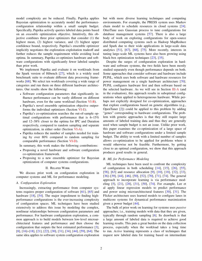
2) Active Learning: To train a model with limited samples,Paprika applies active learning to iteratively query samplesover successive rounds. During each round, the goal is tocollect sample that will improve the model predictions as muchas possible. After collecting and evaluating the sample, themodel is updated and the next round begins. In this process,the key is to come up with a query function that convergesquickly so that Paprika can find the optimal configuration withlimited samples. This is not trivial because the model needsto balance the tradeoff between exploration—avoiding localoptima—and exploitation—improving the predictions of thehighest performance configurations found so far. Prior workhas identified three commonly used optimizers. For practicalsystems optimization, we find that none of the three is alwaysbest and thus we propose an ensemble approach that combinesthem all to improve the predictions. We first review the threecommon optimizers used in prior work and then describePaprika’s ensemble optimizer.

a) Global Optimizer: At each round t, assume the config-uration is xt and its posterior of the GP over f has mean µt(x)and variance σ2

t (x). A standard approach for active learning isto query data points with the maximum information gain [11],which is equivalent to the maximum uncertainty:

xt = arg maxx∈D

σt−1(x). (4)

The intuition is that by picking points with the largest varianceor least confidence so far, it will improve the predictionaccuracy for all future data points by escaping local optima.However, this rule can be wasteful: it aims at decreasinguncertainty globally, not where the maxima might be [53].

Algorithm 1 Bayesian optimization for configuration search.Require: B . All augmented configuration samplesRequire: A0 . Seed augmented configurations setRequire: Y0 . Seed outcome set for seed augmented configurationsRequire: T . Total sample budget

Evaluation set C0 ← B \ A0for each round t = 1, . . . ,T do

Compute mean and variance for samples in Ct−1 by GP.if t mod 3 == 0 then

Pick xt based on the optimizer in Equation 4.else if t mod 3 == 1 then

Pick xt based on the optimizer in Equation 5.else if t mod 3 == 2 then

Pick xt based on the optimizer in Equation 6.Run to get true yt for xt .Update seed configuration set At ← At−1 ∪ xt .Update seed outcome set Yt ← Yt−1 ∪ yt .Update evaluation set Ct ← Ct−1 \ xt .

Output: xT with the maximum predicted mean.

b) Greedy Optimizer: An alternative approach is to op-timize locally by querying data points with the maximumpredicted performance at each step:

xt = arg maxx∈D

µt−1(x). (5)

The intuition is that by picking points with the best perfor-mance so far, it will improve the prediction accuracy for futuredata points with high performance as well. However, this ruleis greedy and tends to get stuck in local optima.

c) Combined Optimizer: To overcome the limitations oftwo query strategies above, a combined approach is:

xt = arg maxx∈D

µt−1(x) + σt−1(x), (6)

which picks xt with the maximum upper confidence bound ateach round. This objective prefers both points x where f isuncertain (large σt−1(x)) and such where we expect to achievehigh performance (large µt−1(x)). This sampling rule greedilyselects points x such that f (x) should be a reasonable upperbound on f (x?).

d) Paprika’s Ensemble Optimizer: To take advantages ofthe merits of the three optimizers above, Paprika proposes anensemble optimizer by choosing each optimizer alternativelyat each round. The intuition is that the ensemble models canproduce better predictive performance compared to a singlemodel, an observation found for other learning systems appliedto other problems [45], [48]. Algorithm 1 summarizes theconfiguration search process for Paprika via the Bayesianapproach. With the ensemble optimizer, Paprika addressesIssue (2) by searching the optimal configuration with limitedsamples as rapidly as possible.Remarks. For the above objectives including Equation 4, 5,and 6, we use arg max when higher performance in magnitudeis better, like IPC. When lower value is better like Duration,

6

we use arg min and the corresponding three objectives will be

xt = arg minx∈D

σt−1(x),

xt = arg minx∈D

µt−1(x),

xt = arg minx∈D

µt−1(x) − σt−1(x).

D. Discussion and Limitations

To query significantly fewer samples, Paprika updates theBayesian optimization models at each round after evaluatingeach query. This update requires extra time cost, which isT times of one round modeling (T is the sample size). Analternative is random sampling evaluating all samples at onceto pick the configuration with highest predicted performance.The random sampling strategy strategy requires fewer modelupdates but can suffer because it does not sample the mostinformative configurations (as would be found by our ensem-ble optimizer). Paprika makes the tradeoff that more modelupdates are better because active learning reduces the totalnumber of samples required, and sample collection is usuallymuch more time-consuming than model updates. Specifically,collecting performance data for a sample usually takes 10–1000 seconds (as measured on our test systems), while updat-ing model once for a sample only takes less than 1 second (seedetails in Section VI-F). In addition, random sampling needsmore than 7 times the samples to achieve equivalent resultscompared to Paprika (see details in Section VI-D). Therefore,it is a huge win to update model at each round after selectinga small size of informative samples compared to collectinga large size of data for random sampling and doing a singlemodel update.

E. Implementation

We implement Paprika as a scheduler for Spark workloads(although we believe the approach should generalize to otherconfigurable software systems) on heterogeneous hardware.The scheduler’s job is to use the model described above toselect the highest performance configuration (of hardware andsoftware) for a given workload. The scheduler then sets theappropriate configuration parameters and runs the Spark jobon the hardware it selects. In this sense, the scheduler isdifferent than typical approaches as users simply input jobs(in the default Spark configuration) and Paprika selects boththe software configuration and the hardware to run it on.

Specifically, we implement Paprika on top of Spark2.2.3 [69], which is an open-source distributed computingframework with a large number of configuration parameters.We evaluate Paprika on workloads from HiBench [27], whichis a widely used benchmark suite for large-scale computingframework. We implement Paprika with Python 3.6, whichis a programming language and environment for statisticalcomputing. The Python packages we use are numpy [25],pandas [40], and scikit-learn [41].

Paprika needs to be trained before deployment. First, weuse Python to generate a Spark configuration list based onEquation 1 and a random value within the value range is also

generated for each configuration parameter. Then, we writePython scripts to run the workloads from Spark version ofHiBench at all configurations in the list on different hardwareand collect their performance data. We concatenate softwareconfigurations and hardware labels in the form of augmentedconfigurations as Equation 2. Then, we run Lasso in Python toselect parameters based on the augmented configurations andtheir performances to reduce the configuration space. Then,we pick the sample budget and seed set, and run Algorithm 1in Python to search the optimal augmented configuration.Once Paprika has performance predictions, it simply schedulesjobs by selecting the configuration with highest predictedperformance for each job.

V. Experimental Setup

A. Systems

We run experiments from a public heterogeneous cloudsystem: the Chameleon Cloud Research Platform [29]. We usethe names that Chameleon 3 uses for three Intel x86 processorswith details shown in Table I.

TABLE I: Details of the hardware microarchitectures.

Skylake Haswell Storage

Processor Gold 6126 E5-2670 E5-2650RAM size 192 GB 128 GB 64 GB# of Threads 48 48 40Clockspeed 2.6 GHz 3.1 GHz 3.0 GHzL3 cache 19.25 M 30 M 25 MMemory speed 2.666 GHz 2.133 GHz 2.133 GHz# Mem channels 6 4 4Network speed 10 GbE 0.1 GbE 10 GbEDisk vendor Samsung Seagate SeagateDisk model MZ7KM240HMHQ0D3 ST9250610NS ST2000NX0273# Disks 1 1 16Disk bandwidth 6 Gb/s 6 Gb/s 24 Gb/s

We use Spark 2.2.3 4 as our software distributed computingframework. Each experiment has a master node and fourworker nodes. We choose a wide range of Spark configurationparameters that reflect significant Spark properties catego-rized by shuffle behavior, data compression and serialization,memory management, execution behavior, networking, andscheduling. Table III shows the total 20 parameters in detail.We use similar parameters to prior work [68] but not thesame set because Spark has actually reduced the number ofuser visible configuration parameters. In part this reductionwas done because proper configuration is such a burden forusers [57].

B. Workloads

We select 10 workloads from the HiBench big data bench-mark suite [27] with details are shown in Table II. Theseworkloads cover various domains including microbenchmarks(micro), machine learning (ML), websearch, and graph, andexhibit a wide range of resource usage.

3https://www.chameleoncloud.org/hardware/4https://spark.apache.org/docs/2.2.3/configuration.html

7

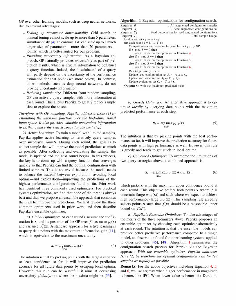
TABLE II: Details of the evaluated workloads.

Workload Category Data size (GB) Resource need

wordcount micro 32 CPUterasort micro 3.2 CPU, memoryals ML 0.6 disk IObayes ML 19 memorykmeans ML 20 memorylr ML 8 CPUlinear ML 48 disk IOrf ML 0.8 disk IOpagerank websearch 1.5 disk IOnweight graph 0.9 CPU, memory

C. Points of Comparisons

We compare the following approaches:• Default: pick the default software configuration on the

default hardware.• HS: pick the available hardware first, and then search for

the best software configuration.• SH: pick the best seen software configuration first, and

then search for the best hardware.• RND: co-optimization by random sampling approach on

the augmented configurations.• Paprika: co-optimization by the proposed Bayesian opti-

mization approach on the augmented configurations.• OPT: exhaustive search for true optimal configuration.

The default hardware is Skylake, which is also the newest.HS and SH optimize hardware and software configurationsseparately in different orders. HS, a similar approach toPUPiL [70], also uses Bayesian optimization approach witha sample budget. RND and Paprika co-optimize hardware andsoftware configurations with the same sample budget whileRND uses random sampling as in the prior work [68].

D. Evaluation Metrics

For each workload, we compare the normalized differencebetween the best achieved performance and the true optimalperformance (found through exhaustive search). We examineboth IPC and Duration to demonstrate that our approachgeneralizes to different outcomes. For IPC, we compute howmuch the predicted value is below the optimal IPC due to thefact that the higher IPC is better:

normalized IPC = 100% ∗(1 −

Ipred

Iopt

), (7)

where Ipred is the best IPC from one of the above methods andIopt is the optimal IPC. We subtract it from 1 so that this metricshows the percentage of predicted IPC below the optimal.

For Duration, we compute how much the predicted valueis above the optimal Duration due to the fact that the lowerDuration is better:

normalized Duration = 100% ∗(

Dpred

Dopt− 1

), (8)

where Dpred is the best predicted Duration from the abovemethods and Dopt is the optimal Duration. Again, we subtract 1

so that this metric shows the percentage of predicted Durationabove the optimal.

E. Evaluation Methodology

We generate a list of configurations using the method de-scribed in Section IV, where we generate 2000 configurationsfor each hardware architecture—6000 configurations in total.For each workload, we run it in each configuration to recordtheir performances including IPC and Duration. Specifically,IPC is monitored by the Linux profiling tool Perf [13] andDuration is recored by HiBench automatically. The optimalsoftware configuration and hardware specification for Durationand IPC are obtained via exhaustive search. It is worth notingthat even for the same workload, the optimal hardware andsoftware configurations for IPC and Duration are different.We then use the algorithms mentioned above to search thebest configurations for a given workload. The default samplebudget is 100, which is much smaller than the prior work usingthousands of sampled configurations [68]. The size of initialseed set is 20. For Bayesian optimization, we use Gaussiankernel for Gaussian Process modeling. All parameters forLasso and Gaussian Process modeling are chosen via crossvalidations. Finally, we compare the IPC and Duration of high-est performances to those from the true optimal configuration.We report the results averaged over 5 runs with different initialsample seeds per workload to eliminate randomness.

VI. Experimental Evaluation

We empirically evaluate the following questions:1) How close are Paprika’s results to the optima?2) How do software parameters react to hardware?3) How sensitive is Paprika to the sample budget?4) How many samples does RND need to match Paprika?5) How does Paprika compare to prior optimizers?6) What is Paprika’s overhead?

A. How close are Paprika’s results to the optima?

Table IV shows the performance results for IPC and Du-ration with the predicted best hardware and software con-figurations from different approaches per workload. The lastrow, AVG, shows the average results across all workloads. Tobetter visualize the comparisons, we compute the normalizeddifference between each approach to OPT and show the barcharts results in Fig. 3. The x-axis shows each Spark workload,while the y-axis shows the comparison results between eachapproach to OPT for IPC and Duration, respectively. Loweris better (closer to optimal). The last column, HarMean,shows the harmonic mean results across all workloads. SHis generally better than HS, which is not surprising due to thefact that hardware can have more influence on performancethan the software configurations. Therefore, picking the besthardware after picking the software configuration is morelikely to produce better performance than the other wayround. Although RND co-optimizes hardware and softwareconfigurations as Paprika does, it works poorly because thelimited random samples do not provide enough information

8

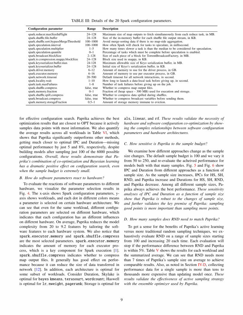
TABLE III: Details of the 20 Spark configuration parameters.

Configuration parameter Range Description

spark.reducer.maxSizeInFlight 24–128 Maximum size of map outputs to fetch simultaneously from each reduce task, in MB.spark.shuffle.file.buffer 24–128 Size of the in-memory buffer for each shuffle file output stream, in KB.spark.shuffle.sort.bypassMergeThreshold 100–1000 Avoid merge-sorting data if there is no map-side aggregation.spark.speculation.interval 100–1000 How often Spark will check for tasks to speculate, in millisecond.spark.speculation.multiplier 1–5 How many times slower a task is than the median to be considered for speculation.spark.speculation.quantile 0–1 Percentage of tasks which must be complete before speculation is enabled.spark.broadcast.blockSize 2–128 Size of each piece of a block for TorrentBroadcastFactory, in MB.spark.io.compression.snappy.blockSize 24–128 Block size used in snappy, in KB.spark.kryoserializer.buffer.max 24-128 Maximum allowable size of Kryo serialization buffer, in MB.spark.kryoserializer.buffer 24–128 Initial size of Kryo’s serialization buffer, in KB.spark.driver.memory 6–12 Amount of memory to use for the driver process, in GB.spark.executor.memory 6–16 Amount of memory to use per executor process, in GB.spark.network.timeout 20–500 Default timeout for all network interactions, in second.spark.locality.wait 1–10 How long to launch a data-local task before giving up, in second.spark.task.maxFailures 1–8 Number of task failures before giving up on the job.spark.shuffle.compress false, true Whether to compress map output files.spark.memory.fraction 0–1 Fraction of (heap space - 300 MB) used for execution and storage.spark.shuffle.spill.compress false, true Whether to compress data spilled during shuffles.spark.broadcast.compress false, true Whether to compress broadcast variables before sending them.spark.memory.storageFraction 0.5–1 Amount of storage memory immune to eviction.

for effective configuration search. Paprika achieves the bestoptimization results that are closest to OPT because it activelysamples data points with most information. We also quantifythe average results across all workloads in Table VI, whichshows that Paprika significantly outperforms other methods,getting much closer to optimal IPC and Duration—missingoptimal performance by just 5 and 8%, respectively, despitebuilding models after sampling just 100 of the 6000 possibleconfigurations. Overall, these results demonstrate that Pa-prika’s combination of co-optimization and Bayesian learninghas a dramatic positive effect on configuration search, evenwhen the sample budget is extremely small.

B. How do software parameters react to hardware?

To evaluate the reactions of software parameters to differenthardware, we visualize the parameter selection results inFig. 4. The x-axis shows Spark configuration parameters, y-axis shows workloads, and each dot in different colors meansa parameter is selected on certain hardware architecture. Wecan see that even for the same workload, different configu-ration parameters are selected on different hardware, whichindicates that each configuration has an different influenceson different hardware. On average, Paprika reduces the modelcomplexity from 20 to 9.2 features by tailoring the soft-ware features to each hardware system. We also notice thatspark.executor.memory and spark.shuffle.compressare the most selected parameters. spark.executor.memoryindicates the amount of memory for each executor pro-cess, which is a key component for Spark execution [1].spark.shuffle.compress indicates whether to compressmap output files. It generally has good effect on perfor-mance because it can reduce the size of data transferred innetwork [12]. In addition, each architecture is optimal forsome subset of workloads. Consider Duration, Skylake isoptimal for bayes kmeans, terasourt, wordcount; Haswellis optimal for lr, nweight, pagerank; Storage is optimal for

als, linear, and rf. These results validate the necessity ofhardware and software configuration co-optimization by show-ing the complex relationships between software configurationparameters and hardware architectures.

C. How sensitive is Paprika to the sample budget?

We examine how different approaches change as the samplesize changes. The default sample budget is 100 and we vary itfrom 50 to 250, and re-evaluate the acheived performance formodels built with that many samples. Fig. 5 and Fig. 6 showIPC and Duration from different approaches as a function ofsample size. As the sample size increases, IPCs for HS, SH,RND, and Paprika increase and Durations for HS, SH, RND,and Paprika decrease. Among all different sample sizes, Pa-prika always achieves the best performance. These sensitivityanalyses of IPC and Duration as a function of sample sizeshow that Paprika is robust to the changes of sample size,and further validates the key premise of Paprika: samplinggood points is more important than sampling more points.

D. How many samples does RND need to match Paprika?

To get a sense for the benefits of Paprika’s active learningversus more traditional random sampling techniques, we ex-haustively evaluate RND on a range of sample sizes startingfrom 100 and increasing 20 each time. Each evaluation willstop if the performance difference between RND and Paprikais within 5%. Table V shows the results for each workload andthe summarized average. We can see that RND needs morethan 7 times of Paprika’s sample size on average to achievecomparable results. Also, as noted in Section IV-D, collectingperformance data for a single sample is more than tens tothousands more expensive than updating model once. Theseresults validate the effectiveness of active sampling strategywith the ensemble optimizer used by Paprika.

9

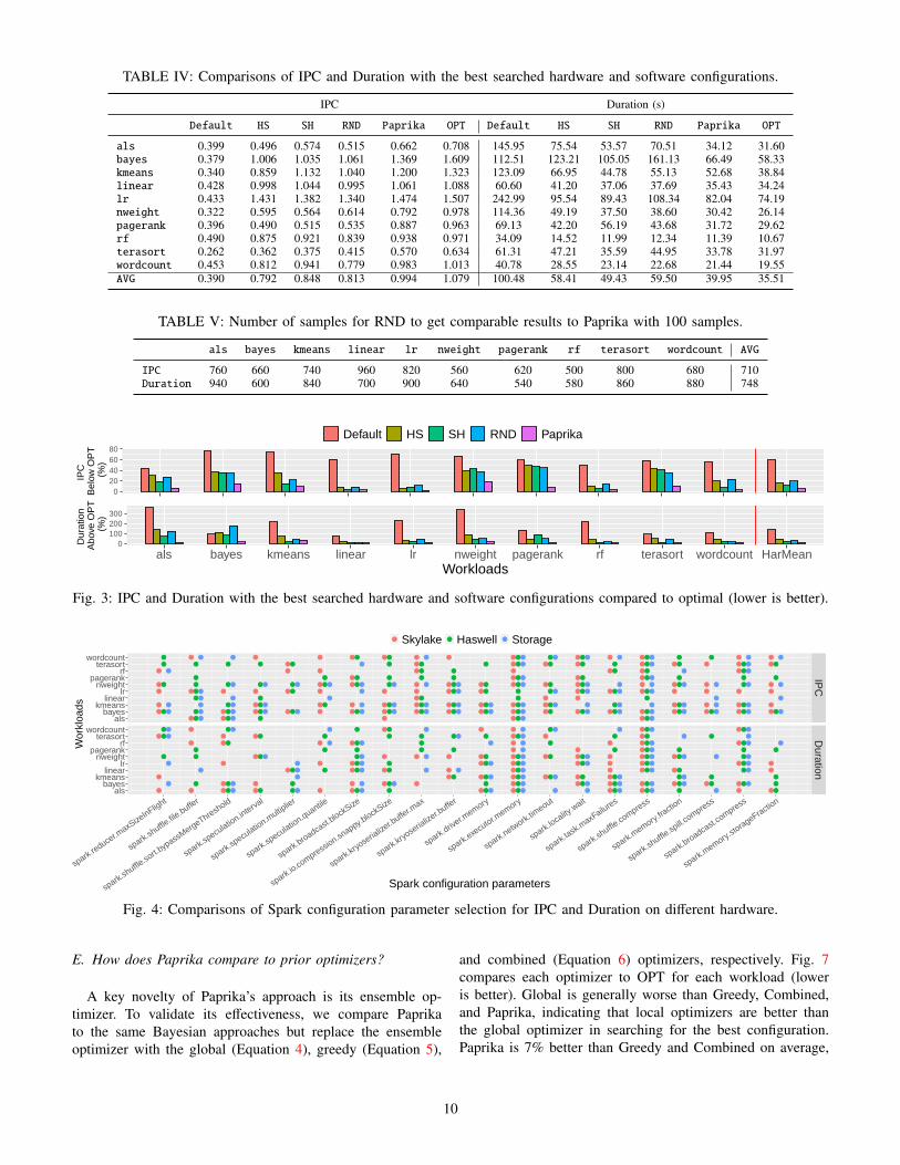
TABLE IV: Comparisons of IPC and Duration with the best searched hardware and software configurations.

IPC Duration (s)

Default HS SH RND Paprika OPT Default HS SH RND Paprika OPT

als 0.399 0.496 0.574 0.515 0.662 0.708 145.95 75.54 53.57 70.51 34.12 31.60bayes 0.379 1.006 1.035 1.061 1.369 1.609 112.51 123.21 105.05 161.13 66.49 58.33kmeans 0.340 0.859 1.132 1.040 1.200 1.323 123.09 66.95 44.78 55.13 52.68 38.84linear 0.428 0.998 1.044 0.995 1.061 1.088 60.60 41.20 37.06 37.69 35.43 34.24lr 0.433 1.431 1.382 1.340 1.474 1.507 242.99 95.54 89.43 108.34 82.04 74.19nweight 0.322 0.595 0.564 0.614 0.792 0.978 114.36 49.19 37.50 38.60 30.42 26.14pagerank 0.396 0.490 0.515 0.535 0.887 0.963 69.13 42.20 56.19 43.68 31.72 29.62rf 0.490 0.875 0.921 0.839 0.938 0.971 34.09 14.52 11.99 12.34 11.39 10.67terasort 0.262 0.362 0.375 0.415 0.570 0.634 61.31 47.21 35.59 44.95 33.78 31.97wordcount 0.453 0.812 0.941 0.779 0.983 1.013 40.78 28.55 23.14 22.68 21.44 19.55AVG 0.390 0.792 0.848 0.813 0.994 1.079 100.48 58.41 49.43 59.50 39.95 35.51

TABLE V: Number of samples for RND to get comparable results to Paprika with 100 samples.

als bayes kmeans linear lr nweight pagerank rf terasort wordcount AVG

IPC 760 660 740 960 820 560 620 500 800 680 710Duration 940 600 840 700 900 640 540 580 860 880 748

Default HS SH RND Paprika

020406080

IPC

B

elow

OP

T

(%

)

0100200300

als bayes kmeans linear lr nweight pagerank rf terasort wordcount HarMeanWorkloads

Dur

atio

n A

bove

OP

T

(%

)

Fig. 3: IPC and Duration with the best searched hardware and software configurations compared to optimal (lower is better).

● ● ● ● ●● ● ● ● ●● ● ● ●

● ● ● ● ● ● ● ● ● ● ● ● ● ● ● ● ● ● ●● ● ● ● ● ● ● ● ● ● ● ● ● ● ● ● ● ● ●● ● ● ● ● ● ● ● ● ● ● ● ● ● ● ● ● ●

● ● ● ● ● ● ● ● ● ● ● ● ● ●● ● ● ● ● ● ● ● ● ● ● ●● ● ● ● ● ● ● ● ● ● ● ● ● ● ● ● ●

● ● ●● ● ● ● ●● ● ● ● ●

● ● ● ● ● ● ● ● ● ● ● ● ● ● ● ● ●● ● ● ● ● ● ● ● ●● ● ● ● ● ● ●

● ● ● ● ● ● ● ● ● ● ● ● ●● ● ● ● ● ● ● ● ● ● ● ● ● ● ●● ● ● ● ● ● ● ● ● ● ● ● ● ● ● ●

● ● ● ●● ● ● ● ● ● ● ● ● ● ● ●● ●

● ● ● ● ● ● ● ●● ● ● ● ●● ● ●

● ● ● ● ● ● ● ● ● ●● ● ● ● ● ● ● ● ● ● ● ● ● ● ● ●● ● ● ●

● ● ● ● ● ● ● ● ● ● ● ● ●● ● ● ● ● ● ● ● ●● ● ● ● ● ● ● ● ● ●

● ● ● ● ● ● ● ● ● ● ● ●● ● ● ● ● ● ● ● ● ● ●● ● ● ● ● ● ● ● ● ●

● ● ● ● ● ● ● ● ● ● ● ●● ● ● ● ● ● ● ● ● ● ● ● ●● ● ● ● ● ● ● ● ● ●

● ● ● ● ● ● ●● ● ● ● ● ● ● ● ●● ● ● ● ● ●

● ● ● ● ● ● ● ● ●● ● ● ● ● ● ● ●● ● ● ● ● ● ● ●

● ● ● ● ● ● ● ● ● ●● ● ● ● ● ● ●● ● ● ● ● ● ● ●

● ● ● ● ● ● ● ● ● ● ●● ● ● ● ● ● ● ● ● ● ●● ● ● ● ● ● ● ● ●

● ● ●● ● ● ● ● ● ● ● ● ●● ●

● ● ● ● ● ● ● ●● ● ● ● ● ●● ● ● ● ● ● ●

● ● ● ● ● ●● ● ● ● ● ● ● ● ● ● ●● ● ● ● ●

● ● ● ● ● ●● ● ● ● ● ● ●● ● ● ● ● ● ● ● ●

IPC

Duration

spark.

reducer.m

axSize

InFlight

spark.

shuffle

.file.buffe

r

spark.

shuffle

.sort.b

ypassM

ergeThreshold

spark.

specu

lation.in

terval

spark.

specu

lation.m

ultiplier

spark.

specu

lation.quantile

spark.

broadcast.

blockSize

spark.

io.compressi

on.snappy.b

lockSize

spark.

kryose

rialize

r.buffe

r.max

spark.

kryose

rialize

r.buffe

r

spark.

driver.m

emory

spark.

execu

tor.memory

spark.

network.tim

eout

spark.

locality

.wait

spark.

task.maxF

ailures

spark.

shuffle

.compress

spark.

memory.fra

ction

spark.

shuffle

.spill.c

ompress

spark.

broadcast.

compress

spark.

memory.sto

rageFraction

alsbayes

kmeanslinear

lrnweight

pagerankrf

terasortwordcount

alsbayes

kmeanslinear

lrnweight

pagerankrf

terasortwordcount

Spark configuration parameters

Wor

kloa

ds

● ● ●Skylake Haswell Storage

Fig. 4: Comparisons of Spark configuration parameter selection for IPC and Duration on different hardware.

E. How does Paprika compare to prior optimizers?

A key novelty of Paprika’s approach is its ensemble op-timizer. To validate its effectiveness, we compare Paprikato the same Bayesian approaches but replace the ensembleoptimizer with the global (Equation 4), greedy (Equation 5),

and combined (Equation 6) optimizers, respectively. Fig. 7compares each optimizer to OPT for each workload (loweris better). Global is generally worse than Greedy, Combined,and Paprika, indicating that local optimizers are better thanthe global optimizer in searching for the best configuration.Paprika is 7% better than Greedy and Combined on average,

10

●● ● ● ●

●

● ● ● ●● ● ● ●

●●

● ● ● ●● ● ● ● ●

●●

● ● ●

●

● ● ● ●● ● ● ● ●

● ● ● ● ●● ● ● ● ●

● ● ● ● ●

●

● ● ● ●● ● ● ●

●

● ● ● ● ●● ● ● ● ●

● ● ● ● ●

●

● ● ● ●● ● ● ● ●

● ●● ● ●● ● ● ● ●

● ● ● ● ●

●

● ● ● ●● ● ● ● ●● ● ● ● ●● ● ● ● ●

● ● ● ● ●

●

● ● ● ●

● ● ●● ●

●● ● ● ●● ● ● ● ●

●●

● ● ●

●

● ● ● ●

●● ● ● ●

●● ● ● ●

● ● ● ● ●

● ● ● ● ●

●

● ● ● ●●

● ● ●●

● ● ●

● ●● ● ● ● ●

● ● ●● ●

●

● ● ● ●

● ● ● ● ●

● ● ● ● ●● ● ● ● ●

● ● ● ●●

●

● ● ● ●

●●

●● ●

● ● ● ● ●● ● ● ● ●

nweight pagerank rf terasort wordcount

als bayes kmeans linear lr

50 100 150 200 250 50 100 150 200 250 50 100 150 200 250 50 100 150 200 250 50 100 150 200 250

1.21.31.41.5

0.750.800.850.900.951.00

0.850.900.951.001.051.10

0.30.40.50.6

0.91.01.11.21.3

0.8

0.9

1.11.31.5

0.4

0.6

0.8

0.5

0.6

0.7

0.50.60.70.80.91.0

Sample Size

IPC

● ● ● ● ●HS SH RND Paprika OPT

Fig. 5: Sensitivity analysis of IPC with different sample size per workload.

●

● ● ● ●● ● ● ● ●

● ●

● ● ●

● ● ● ● ●● ● ● ● ●

●● ● ● ●

● ● ● ● ●● ● ● ● ●● ● ● ● ●● ● ● ● ●

●●

●●

●● ● ● ● ●

●●

● ● ●

● ● ● ● ●● ● ● ● ●

●● ● ● ●

●● ● ● ●●

● ●●

●●● ●

● ●● ● ● ● ●

●●

●

●●● ● ● ● ●

●

● ● ● ●● ● ● ● ●● ● ● ● ●

● ● ● ● ●

●● ● ● ●

●●

● ● ●

● ●● ●

●● ● ● ● ●

● ● ●

●●

●

● ●●

●

●

● ● ● ●● ● ● ● ●● ● ● ● ●

●

●● ●

●●

● ● ● ●

● ●●

● ●●● ● ● ●

● ● ● ● ●

● ●●

●●●

● ● ● ●

●

●● ● ●

●● ● ● ●

● ● ● ● ●

●●

●● ●

●● ● ● ●

●● ● ●

●● ● ● ● ●

● ● ● ● ●

nweight pagerank rf terasort wordcount

als bayes kmeans linear lr

50 100 150 200 250 50 100 150 200 250 50 100 150 200 250 50 100 150 200 250 50 100 150 200 250

8090

100110120

20242832

3436384042

354045

406080

100

11121314

100

150

30405060

3040506070

30405060

Sample Size

Dur

atio

n (s

)

● ● ● ● ●HS SH RND Paprika OPT

Fig. 6: Sensitivity analysis of Duration with different sample size per workload.

Global Greedy Combined Paprika

05

101520

IPC

B

elow

OP

T

(%

)

0

20

40

60

80

alsbayes

kmeanslinear lr

nweightpagerank rf

terasort

wordcountHarMean

Workloads

Dur

atio

n A

bove

OP

T

(%

)

Fig. 7: Comparing Paprika to prior optimizers.

HS SH RND Paprika

0

200

400

600

Tim

e (m

s)

0

200

400

600

alsbayes

kmeanslinear lr

nweightpagerank rf

terasort

wordcountAVG

Workloads

Tim

e (m

s)

Fig. 8: Overheads for different approaches.

TABLE VI: Harmonic mean of normalized IPC and normal-ized Duration for different approaches. Lower is better.

Default HS SH RND Paprika

IPC 60% 16% 11% 20% 5%Duration 142% 46% 20% 29% 8%

which validates the effectiveness of Paprika’s ensemble opti-mizer’s ability to balance the exploration–exploitation tradeoff.The reason that the ensemble optimizer triumphs is thatit generally reduce variances and avoids overfitting. Theseresults show that Paprika is effective in balancing the tradeoff

between exploring, exploitation, and optimizing.

F. What is Paprika’s overhead?

We collect overheads for each approach in Fig. 8, whichshows the running time per approach per workload on a Sky-lake machine. RND is the computational cheapest compared

to the other methods, which is not surprising because randomsampling barely costs anything, while the other three methodsactively sample points to iteratively update the model. Paprikahas a slightly higher overhead than HS and SH because ithandles extra hardware dimensional features for optimizationdue to the designed augmented configurations. These resultsshow that Paprika searches much better configuration with aslight higher overheads compared to other approaches.

VII. Conclusion

This paper introduces Paprika, a scheduler that selectshardware and software configurations simultaneously basedon models learned from an extremely limited sample budget.Paprika’s key observation is that a given workload has dif-ferent optimal software configurations on different hardware.Therefore, Paprika devises a novel and efficient configurationaugmentation approach to achieve hardware and software con-figuration co-optimization. Paprika also proposes a Bayesian

11

approach with the ensemble optimizer for fast configurationsearch such that only a small sample budget is needed. Wefind that Paprika searches the optimal hardware and softwareconfigurations effectively and efficiently with fewer samplescompared to (1) optimizing hardware and software configura-tions individually, (2) random sampling, and (3) prior optimiz-ers. This work is strong evidence that optimizing performanceshould consider both hardware and software configurations,especially in heterogeneous computing environments. We hopethis work inspires architecture and system researchers toconsider the cross-stack features before applying learning tosolve problems.

12

References

[1] D. M. Adinew, Z. Shijie, and Y. Liao, “Spark performance optimizationanalysis in memory management with deploy mode in standalone clustercomputing,” in 2020 IEEE 36th International Conference on DataEngineering (ICDE). IEEE, 2020, pp. 2049–2053.

[2] J. Ansel, S. Kamil, K. Veeramachaneni, J. Ragan-Kelley, J. Bosboom,U.-M. O’Reilly, and S. Amarasinghe, “Opentuner: An extensible frame-work for program autotuning,” in Proceedings of the 23rd internationalconference on Parallel architectures and compilation, 2014, pp. 303–316.

[3] J. Ansel, M. Pacula, Y. L. Wong, C. Chan, M. Olszewski, U.-M. O’Reilly, and S. Amarasinghe, “Siblingrivalry: online autotuningthrough local competitions,” in CASES, 2012.

[4] J. Bergstra and Y. Bengio, “Random search for hyper-parameter opti-mization,” The Journal of Machine Learning Research, vol. 13, no. 1,pp. 281–305, 2012.

[5] R. Bitirgen, E. Ipek, and J. F. Martinez, “Coordinated managementof multiple interacting resources in chip multiprocessors: A machinelearning approach,” in 2008 41st IEEE/ACM International Symposiumon Microarchitecture. IEEE, 2008, pp. 318–329.

[6] J. G. Carbonell, R. S. Michalski, and T. M. Mitchell, “An overview ofmachine learning,” in Machine learning. Elsevier, 1983, pp. 3–23.

[7] A. Carroll and G. Heiser, “Mobile multicores: Use them or wastethem,” in Proceedings of the Workshop on Power-Aware Computing andSystems, 2013, pp. 1–5.

[8] S. Che, M. Boyer, J. Meng, D. Tarjan, J. W. Sheaffer, S.-H. Lee, andK. Skadron, “Rodinia: A benchmark suite for heterogeneous computing,”in IISWC, 2009.

[9] S. Choi and D. Yeung, “Learning-based smt processor resource distribu-tion via hill-climbing,” in 33rd International Symposium on ComputerArchitecture (ISCA’06). IEEE, 2006, pp. 239–251.

[10] R. Cochran, C. Hankendi, A. K. Coskun, and S. Reda, “Pack &cap: adaptive dvfs and thread packing under power caps,” in 201144th Annual IEEE/ACM International Symposium on Microarchitecture(MICRO). IEEE, 2011, pp. 175–185.

[11] T. M. Cover, Elements of information theory. John Wiley & Sons,1999.

[12] A. Davidson, “Optimizing shuffle performance in spark,” 2013.[13] A. C. De Melo, “The new linux’perf’tools,” in Slides from Linux

Kongress, vol. 18, 2010, pp. 1–42.[14] C. Delimitrou and C. Kozyrakis, “Paragon: Qos-aware scheduling for

heterogeneous datacenters,” ACM SIGPLAN Notices, vol. 48, no. 4, pp.77–88, 2013.

[15] C. Delimitrou and C. Kozyrakis, “Quasar: resource-efficient and qos-aware cluster management,” ACM SIGPLAN Notices, vol. 49, no. 4, pp.127–144, 2014.

[16] Z. Deng, L. Zhang, N. Mishra, H. Hoffmann, and F. T. Chong, “Memorycocktail therapy: a general learning-based framework to optimize dy-namic tradeoffs in nvms,” in Proceedings of the 50th Annual IEEE/ACMInternational Symposium on Microarchitecture, 2017, pp. 232–244.

[17] A. S. Dhodapkar and J. E. Smith, “Managing multi-configuration hard-ware via dynamic working set analysis,” in Proceedings 29th AnnualInternational Symposium on Computer Architecture. IEEE, 2002, pp.233–244.

[18] Y. Ding, N. Mishra, and H. Hoffmann, “Generative and multi-phaselearning for computer systems optimization,” in Proceedings of the 46thInternational Symposium on Computer Architecture, 2019, pp. 39–52.

[19] S. Duan, V. Thummala, and S. Babu, “Tuning database configurationparameters with ituned,” Proceedings of the VLDB Endowment, vol. 2,no. 1, pp. 1246–1257, 2009.

[20] C. Dubach, T. M. Jones, E. V. Bonilla, and M. F. P. O’Boyle, “Apredictive model for dynamic microarchitectural adaptivity control,” inProceedings of the 43rd Annual International Symposium on Microar-chitecture, ser. MICRO’43, 2010, pp. 485–496.

[21] C. Dubach, T. M. Jones, E. V. Bonilla, and M. F. O’Boyle, “A predic-tive model for dynamic microarchitectural adaptivity control,” in 201043rd Annual IEEE/ACM International Symposium on Microarchitecture.IEEE, 2010, pp. 485–496.

[22] A. Ganapathi, K. Datta, A. Fox, and D. Patterson, “A case for machinelearning to optimize multicore performance,” in Proceedings of the FirstUSENIX conference on Hot topics in parallelism. USENIX AssociationBerkeley, CA, 2009, pp. 1–1.

[23] D. Golovin, B. Solnik, S. Moitra, G. Kochanski, J. Karro, and D. Sculley,“Google vizier: A service for black-box optimization,” in Proceedingsof the 23rd ACM SIGKDD international conference on knowledgediscovery and data mining, 2017, pp. 1487–1495.

[24] Z. Gong, X. Gu, and J. Wilkes, “Press: Predictive elastic resource scalingfor cloud systems,” in 2010 International Conference on Network andService Management. Ieee, 2010, pp. 9–16.

[25] C. R. Harris, K. J. Millman, S. J. van der Walt, R. Gommers, P. Virtanen,D. Cournapeau, E. Wieser, J. Taylor, S. Berg, N. J. Smith, R. Kern,M. Picus, S. Hoyer, M. H. van Kerkwijk, M. Brett, A. Haldane,J. Fernandez del Rıo, M. Wiebe, P. Peterson, P. Gerard-Marchant,K. Sheppard, T. Reddy, W. Weckesser, H. Abbasi, C. Gohlke, andT. E. Oliphant, “Array programming with numpy,” Nature, vol. 585,p. 357–362, 2020.

[26] H. Hoffmann, “Jouleguard: energy guarantees for approximate applica-tions,” in Proceedings of the 25th Symposium on Operating SystemsPrinciples, 2015, pp. 198–214.

[27] S. Huang, J. Huang, Y. Liu, L. Yi, and J. Dai, “Hibench: A representativeand comprehensive hadoop benchmark suite,” in Proc. ICDE Workshops,2010, pp. 41–51.

[28] E. Ipek, O. Mutlu, J. F. Martınez, and R. Caruana, “Self-optimizingmemory controllers: A reinforcement learning approach,” in Proceedingsof the 35th Annual International Symposium on Computer Architecture,ser. ISCA’08, USA, 2008, pp. 39–50.

[29] K. Keahey, J. Anderson, Z. Zhen, P. Riteau, P. Ruth, D. Stanzione,M. Cevik, J. Colleran, H. S. Gunawi, C. Hammock, J. Mambretti,A. Barnes, F. Halbach, A. Rocha, and J. Stubbs, “Lessons learned fromthe chameleon testbed,” in Proceedings of the 2020 USENIX AnnualTechnical Conference (USENIX ATC ’20). USENIX Association, July2020.

[30] B. C. Lee and D. Brooks, “Applied inference: Case studies in mi-croarchitectural design,” ACM Transactions on Architecture and CodeOptimization (TACO), vol. 7, no. 2, pp. 1–37, 2010.

[31] B. C. Lee and D. M. Brooks, “Accurate and efficient regression mod-eling for microarchitectural performance and power prediction,” ACMSIGOPS operating systems review, vol. 40, no. 5, pp. 185–194, 2006.

[32] B. C. Lee, D. M. Brooks, B. R. de Supinski, M. Schulz, K. Singh,and S. A. McKee, “Methods of inference and learning for performancemodeling of parallel applications,” in Proceedings of the 12th ACM SIG-PLAN symposium on Principles and practice of parallel programming,2007, pp. 249–258.

[33] B. C. Lee, J. Collins, H. Wang, and D. Brooks, “Cpr: Composableperformance regression for scalable multiprocessor models,” in 200841st IEEE/ACM International Symposium on Microarchitecture. IEEE,2008, pp. 270–281.

[34] J. Li and J. F. Martinez, “Dynamic power-performance adaptation ofparallel computation on chip multiprocessors,” in The Twelfth Interna-tional Symposium on High-Performance Computer Architecture, 2006.IEEE, 2006, pp. 77–87.

[35] L. Li, K. Jamieson, G. DeSalvo, A. Rostamizadeh, and A. Talwalkar,“Hyperband: A novel bandit-based approach to hyperparameter opti-mization,” The Journal of Machine Learning Research, vol. 18, no. 1,pp. 6765–6816, 2017.

[36] J. F. Martinez and E. Ipek, “Dynamic multicore resource management:A machine learning approach,” IEEE micro, vol. 29, no. 5, pp. 8–17,2009.

[37] N. Mishra, C. Imes, J. D. Lafferty, and H. Hoffmann, “Caloree: Learningcontrol for predictable latency and low energy,” in Proceedings of theTwenty-Third International Conference on Architectural Support forProgramming Languages and Operating Systems, ser. ASPLOS’18, NewYork, NY, USA, 2018, pp. 184–198.

[38] N. Mishra, H. Zhang, J. D. Lafferty, and H. Hoffmann, “A proba-bilistic graphical model-based approach for minimizing energy underperformance constraints,” in Proceedings of the Twentieth InternationalConference on Architectural Support for Programming Languages andOperating Systems, ser. ASPLOS’15, New York, NY, USA, 2015, pp.267–281.

[39] A. J. Oliner, A. P. Iyer, I. Stoica, E. Lagerspetz, and S. Tarkoma, “Carat:Collaborative energy diagnosis for mobile devices,” in Proceedings ofthe 11th ACM Conference on Embedded Networked Sensor Systems,2013, pp. 1–14.

[40] T. pandas development team, “pandas-dev/pandas: Pandas,” Feb. 2020.[41] F. Pedregosa, G. Varoquaux, A. Gramfort, V. Michel, B. Thirion,

O. Grisel, M. Blondel, P. Prettenhofer, R. Weiss, V. Dubourg, J. Vander-

13

plas, A. Passos, D. Cournapeau, M. Brucher, M. Perrot, and E. Duch-esnay, “Scikit-learn: Machine learning in Python,” Journal of MachineLearning Research, vol. 12, pp. 2825–2830, 2011.

[42] D. D. Penney and L. Chen, “A survey of machine learning applied tocomputer architecture design,” arXiv preprint arXiv:1909.12373, 2019.

[43] J. A. Pereira, H. Martin, M. Acher, J.-M. Jezequel, G. Botterweck, andA. Ventresque, “Learning software configuration spaces: A systematicliterature review,” arXiv preprint arXiv:1906.03018, 2019.

[44] P. Petrica, A. M. Izraelevitz, D. H. Albonesi, and C. A. Shoemaker,“Flicker: A dynamically adaptive architecture for power limited multi-core systems,” in Proceedings of the 40th Annual International Sympo-sium on Computer Architecture, 2013, pp. 13–23.

[45] R. Polikar, “Ensemble learning,” in Ensemble machine learning.Springer, 2012, pp. 1–34.

[46] D. Ponomarev, G. Kucuk, and K. Ghose, “Reducing power requirementsof instruction scheduling through dynamic allocation of multiple data-path resources,” in Proceedings. 34th ACM/IEEE International Sympo-sium on Microarchitecture. MICRO-34. IEEE, 2001, pp. 90–101.

[47] P. Rodrıguez, M. A. Bautista, J. Gonzalez, and S. Escalera, “Beyondone-hot encoding: Lower dimensional target embedding,” Image andVision Computing, vol. 75, pp. 21–31, 2018.

[48] H. Sayadi, N. Patel, S. M. PD, A. Sasan, S. Rafatirad, and H. Homayoun,“Ensemble learning for effective run-time hardware-based malwaredetection: A comprehensive analysis and classification,” in 2018 55thACM/ESDA/IEEE Design Automation Conference (DAC). IEEE, 2018,pp. 1–6.

[49] B. Settles, “From theories to queries: Active learning in practice,” inActive Learning and Experimental Design workshop In conjunction withAISTATS 2010, 2011, pp. 1–18.

[50] D. C. Snowdon, E. Le Sueur, S. M. Petters, and G. Heiser, “Koala:A platform for os-level power management,” in Proceedings of the 4thACM European conference on Computer systems, 2009, pp. 289–302.

[51] E. R. Sparks, A. Talwalkar, D. Haas, M. J. Franklin, M. I. Jordan, andT. Kraska, “Automating model search for large scale machine learning,”in Proceedings of the Sixth ACM Symposium on Cloud Computing, 2015,pp. 368–380.

[52] S. Sridharan, G. Gupta, and G. S. Sohi, “Holistic run-time parallelismmanagement for time and energy efficiency,” in Proceedings of the27th international ACM conference on International conference onsupercomputing, 2013, pp. 337–348.

[53] N. Srinivas, A. Krause, S. Kakade, and M. Seeger, “Gaussian processoptimization in the bandit setting: No regret and experimental design,”in Proceedings of the 27th International Conference on InternationalConference on Machine Learning, 2010, p. 1015–1022.

[54] Y. Sun, T. Baruah, S. A. Mojumder, S. Dong, X. Gong, S. Treadway,Y. Bao, S. Hance, C. McCardwell, V. Zhao et al., “Mgpusim: Enablingmulti-gpu performance modeling and optimization,” in Proceedings ofthe 46th International Symposium on Computer Architecture, 2019, pp.197–209.

[55] G. Tesauro, “Reinforcement learning in autonomic computing: A man-ifesto and case studies,” IEEE Internet Computing, vol. 11, no. 1, pp.22–30, 2007.

[56] R. Tibshirani, “Regression shrinkage and selection via the lasso,” Jour-nal of the Royal Statistical Society: Series B (Methodological), vol. 58,no. 1, pp. 267–288, 1996.

[57] D. Van Aken, A. Pavlo, G. J. Gordon, and B. Zhang, “Automaticdatabase management system tuning through large-scale machine learn-ing,” in Proceedings of the 2017 ACM International Conference onManagement of Data, 2017, pp. 1009–1024.

[58] K. Van Craeynest, A. Jaleel, L. Eeckhout, P. Narvaez, and J. Emer,“Scheduling heterogeneous multi-cores through performance impactestimation (pie),” in 2012 39th Annual International Symposium onComputer Architecture (ISCA). IEEE, 2012, pp. 213–224.

[59] S. Venkataraman, Z. Yang, M. Franklin, B. Recht, and I. Stoica, “Ernest:Efficient performance prediction for large-scale advanced analytics,” in13th USENIX Symposium on Networked Systems Design and Implemen-tation (NSDI 16), 2016, pp. 363–378.

[60] K. V. Vishwanath and N. Nagappan, “Characterizing cloud computinghardware reliability,” in Proceedings of the 1st ACM symposium onCloud computing, 2010, pp. 193–204.

[61] S. Wang, C. Li, H. Hoffmann, S. Lu, W. Sentosa, and A. I. Kistijan-toro, “Understanding and auto-adjusting performance-sensitive configu-rations,” ACM SIGPLAN Notices, vol. 53, no. 2, pp. 154–168, 2018.

[62] C. K. Williams and C. E. Rasmussen, Gaussian processes for machinelearning. MIT press Cambridge, MA, 2006, vol. 2, no. 3.

[63] J. A. Winter, D. H. Albonesi, and C. A. Shoemaker, “Scalable threadscheduling and global power management for heterogeneous many-core architectures,” in 2010 19th International Conference on ParallelArchitectures and Compilation Techniques (PACT). IEEE, 2010, pp.29–39.

[64] W. Wu and B. C. Lee, “Inferred models for dynamic and sparsehardware-software spaces,” in 2012 45th Annual IEEE/ACM Interna-tional Symposium on Microarchitecture. IEEE, 2012, pp. 413–424.

[65] T. Xu, L. Jin, X. Fan, Y. Zhou, S. Pasupathy, and R. Talwadker, “Hey,you have given me too many knobs!: understanding and dealing withover-designed configuration in system software,” in Proceedings of the2015 10th Joint Meeting on Foundations of Software Engineering, 2015,pp. 307–319.

[66] T. Xu, X. Jin, P. Huang, Y. Zhou, S. Lu, L. Jin, and S. Pasupathy, “Earlydetection of configuration errors to reduce failure damage,” in 12thUSENIX Symposium on Operating Systems Design and Implementation(OSDI 16), 2016, pp. 619–634.

[67] N. Yigitbasi, T. L. Willke, G. Liao, and D. Epema, “Towards machinelearning-based auto-tuning of mapreduce,” in 2013 IEEE 21st Interna-tional Symposium on Modelling, Analysis and Simulation of Computerand Telecommunication Systems. IEEE, 2013, pp. 11–20.

[68] Z. Yu, Z. Bei, and X. Qian, “Datasize-aware high dimensional configu-rations auto-tuning of in-memory cluster computing,” in Proceedings ofthe Twenty-Third International Conference on Architectural Support forProgramming Languages and Operating Systems, 2018, pp. 564–577.

[69] M. Zaharia, M. Chowdhury, M. J. Franklin, S. Shenker, I. Stoica et al.,“Spark: Cluster computing with working sets.” HotCloud, vol. 10, no.10-10, p. 95, 2010.

[70] H. Zhang and H. Hoffmann, “Maximizing performance under a powercap: A comparison of hardware, software, and hybrid techniques,” ACMSIGPLAN Notices, vol. 51, no. 4, pp. 545–559, 2016.

[71] X. Zhang, R. Zhong, S. Dwarkadas, and K. Shen, “A flexible frameworkfor throttling-enabled multicore management (temm),” in 2012 41stInternational Conference on Parallel Processing. IEEE, 2012, pp. 389–398.

[72] Y. Zhang and Y. Huang, “”learned”: Operating systems,” OperatingSystems Review, vol. 53, no. 1, pp. 40–45, 2019.

[73] Y. Zhang, D. Meisner, J. Mars, and L. Tang, “Treadmill: Attributingthe source of tail latency through precise load testing and statisticalinference,” in 2016 ACM/IEEE 43rd Annual International Symposiumon Computer Architecture (ISCA). IEEE, 2016, pp. 456–468.

[74] Y. Zhu and V. J. Reddi, “High-performance and energy-efficient mobileweb browsing on big/little systems,” in 2013 IEEE 19th InternationalSymposium on High Performance Computer Architecture (HPCA), 2013.

[75] Y. Zhu, J. Liu, M. Guo, Y. Bao, W. Ma, Z. Liu, K. Song, and Y. Yang,“Bestconfig: tapping the performance potential of systems via automaticconfiguration tuning,” in Proceedings of the 2017 Symposium on CloudComputing, 2017, pp. 338–350.

14