Höhle, Held:

Bayesian Estimation of the Size of a Population

Sonderforschungsbereich 386, Paper 499 (2006)

Online unter: http://epub.ub.uni-muenchen.de/

Projektpartner

Bayesian Estimation of the Size of a Population

Michael Höhle∗ Leonhard HeldDepartment of Statistics Biostatistics Unit, ISPM

University of Munich University of ZurichGermany Switzerland

Abstract

We consider the following problem: estimate the size of a population markedwith serial numbers after only a sample of the serial numbers has been ob-served. Its simplicity in formulation and the inviting possibilities of applica-tion make this estimation well suited for an undergraduate level probabilitycourse. Our contribution consists in a Bayesian treatment of the problem.For an improper uniform prior distribution, we show that the posterior meanand variance have nice closed form expressions and we demonstrate how tocompute highest posterior density intervals. Maple and R code is providedon the authors’ web-page to allow students to verify the theoretical resultsand experiment with data.

Keywords: Bayesian inference, Combinatorics, Hypergeometric functions,Maple, R.

1 INTRODUCTION

Assume we have a population of unknown size N which is labeled using the serialnumbers {1, . . . , N}, e.g. the number of participants in a marathon, taxis in a cityor serial markings of a production. A random sample (X1, . . . , Xn) of size n ≤ Nis observed without replacement. Let X = max(X1, . . . , Xn) be the maximum ofthis sample. The task is to make inference for the population size N based on theobserved value of X; throughout the text we shall call this the SNP-problem.

A fascinating historic report about the application of this type of population sizeestimation in economical intelligence during World War II is given by Ruggles and

∗Department of Statistics, University of Munich, Ludwigstr. 33, 80539 München, Germany,Email: hoehle@stat.uni-muenchen.de

1

Brodie (1947). The corresponding statistical treatment of the topic in a frequentistperspective is given by Goodman (1952, 1954) who derive unbiased minimum vari-ance estimators and confidence intervals. Johnson (1994) treats the SNP-problemin a pedagogical setting and a search on courses pages on the Internet reveals quitea few pages containing relevant lab exercises. This characteristic as a nice appli-cation of statistics is also reflected by popular science literature (Matthews 1998)giving mention to the problem.

Our contribution is to cast the SNP-problem into a Bayesian framework. Basedon prior information about N the posterior distribution of N given the observedvalue X = x is calculated using Bayes formula. This has to some degree beendone earlier by Roberts (1967), however his derivations are done in the context ofstopping rules where the sample size n is not fixed in advance. Our derivations aremore straightforward – a thorough Bayesian treatment is given including computa-tion of highest posterior density intervals and different cases of prior distributions.All derivations are exact, which avoids the usual problems (e.g. convergence, time-usage) of simulation based Bayesian inference.

From a pedagogical point of view the application has, similarly to a Bayesianversion of the capture-recapture experiment, the advantage that all involved distri-butions are discrete thus not requiring any knowledge about continuous distribu-tions. In an undergraduate probability course context it would be possible to let thederivations be part of an exercise on working with symbolic algebra packages likeMaple (MapleSoft 2004) or an exercise in implementing simple solutions in e.g.R (R Development Core Team 2006).

2 MATHEMATICAL SETTING

Methods to make inference about N discussed in the literature cover maximumlikelihood estimation, finding an unbiased estimator, bounding the probability toovershoot the maximum or calculating posterior densities (Goodman 1952, 1954;Roberts 1967; Gum et al. 2000). Independent of the framework, the likelihood forobserving X = x in a sample of size n plays a central role. It is given as

P (x|N) = P (X = x|N) =

(x−1n−1

)(Nn

) , if n ≤ x ≤ N, and 0 otherwise. (1)

In Goodman (1952) the unbiased estimator of N with minimum variance isshown to be

N̂ =n + 1

nx− 1, (2)

2

and a 1− α confidence interval for N is given as [x, x + 1, . . . , Nu], where Nu isthe largest integer satisfying (x)n/(Nu)n ≥ α. Here we have used (x)n to denotethe so called falling factorial, i.e.

(x)n = x!/(x− n)! = x(x− 1) · · · (x− n + 1).

Turning to a Bayesian framework, we assume a suitable prior distribution forN , after which the posterior distribution can be calculated via Bayes’ theorem, i.e.

P (N |x) =P (x|N)P (N)

P (x)=

P (x|N)P (N)∑∞N ′=x P (x|N ′)P (N ′)

(3)

for x ≤ N < ∞ and zero otherwise. Note that (1) implies, that only values of Nwith N ≥ x have positive posterior probability. We therefore let the sum in thedenominator start at x, although the prior may be positive also for smaller valuesof N . In particular, it is irrelevant if the support of the prior distribution starts at 0or at 1. For ease of presentation, we let the prior start at 0.

Various choices can be imagined as prior distribution for N :

• An improper uniform prior on all positive integers, i.e. P (N) ∝ 1 for N =0, . . . ,∞.

• A proper uniform distribution with an upper limit k for N , i.e. P (N) =1/(k + 1) for 0 ≤ N ≤ k and zero otherwise.

• A Geometric, Poisson or Negative Binomial distribution.

3 POSTERIOR PROPERTIES UNDER AN IMPROPERUNIFORM PRIOR

The case of an improper uniform prior is of particular interest. Using theory aboutinfinite binomial series and hypergeometric functions it can be shown that, forn > 1, the posterior distribution is then given as the discrete distribution

P (N |x) =n− 1

x

(x

n

)(N

n

)−1

, if N = x, x + 1, x + 2, . . . , (4)

and 0 otherwise. The above distribution is thus a shifted factorial distribution (Mar-low 1965), i.e. N−x follows a factorial distribution with parameters x and n. Notethat the posterior distribution is improper for n = 1, which we will show below.

It is easy to show that the Maximum Likelihood estimate, i.e. the posteriormode under the improper uniform prior, is N̂ML = x, the smallest N -value of

3

the posterior distribution with positive posterior probability. However, it is perhapsless known that simple formulae also exist for the posterior mean and variance:

E(N |x) =n− 1n− 2

· (x− 1) for n > 2 and (5)

Var(N |x) =(n− 1)(x− 1)(x− n + 1)

(n− 2)2(n− 3)for n > 3. (6)

In the following these results are derived analytically. Results for the posteriorin case of various proper priors are given in Section 5.

3.1 Analytic derivations using binomial sums

Under the assumption of an improper uniform prior, the posterior distribution (3)simplifies to

P (N |x) =

(Nn

)−1∑∞N ′=x

(N ′

n

)−1 (7)

for x ≤ N < ∞ and zero otherwise. The main problem here is to simplify thedenominator, which is an infinite sum of inverse binomial coefficients

(nk

). This

is a case for classic combinatorial theory, but usually the forms treated in the lit-erature are of the type where n is fixed and k varies, e.g. sums like

∑∞k=0

(nk

)−1.Classical combinatorial theory has used various ad-hoc, problem-specific and inge-nious ways to come up with the right solution to finite and infinite binomial sums.A unified framework for handling binomial sums which has become increasinglypopular in the literature are hypergeometric functions.

Barne’s extended hypergeometric function form is given as

pFq

[a1, . . . , ap; b1, . . . , bq; z

]=

∞∑i=0

(a1)i · · · (ap)i

(b1)i · · · (bq)i

zi

i!, (8)

where (x)i are the rising factorials (also called Pochhammer symbols) defined as

(x)i =(x + i− 1)!

(x− 1)!=

Γ(x + i)x

= (x + i− 1) · . . . · x.

Note that x can be negative in the factorials and thus a general definition of thefactorial and the Gamma function is required. Examples of the above definitionsare (1)z = z! and exp(z) = 0F0[z].

There are various results about hypergeometric functions, the most importantwith respect to our problem is Gauss’ hypergeometric function,

2F1

[a, b; c; 1

]=

∞∑i=0

(a)i(b)i

(c)i

1i!

=Γ(c)Γ(c− a− b)Γ(c− a)Γ(c− b)

,

4

and originates as the solution to the so called hypergeometric differential equa-tion (Wolfram Research 2004b).

To compute the sum in the denominator of (7), we now proceed as follows:

∞∑N ′=x

(N ′

n

)−1

=∞∑i=0

(x + i

n

)−1

=∞∑i=0

n!(x + i− n)!(x + i)!

=(

x

n

)−1 ∞∑i=0

x!(x + i)!

(x + i− n)!(x− n)!

=(

x

n

)−1 ∞∑i=0

(x− n + 1)i

(x + 1)i

=(

x

n

)−1 ∞∑i=0

(x− n + 1)i(1)i

(x + 1)i

1i!

=(

x

n

)−1

2F1

[1 + x− n, 1;x + 1; 1

]=

(x

n

)−1 Γ(x + 1)Γ(n− 1)Γ(n)Γ(x)

=(

x

n

)−1 x

n− 1, (9)

where we have used Γ(x+1)/Γ(x) = x at the very end. The form of the posteriordistribution in (4) follows immediately.

Clearly this derivation can only be valid for n ≥ 2. In fact, it is easy to see thatfor n = 1 the posterior is improper, because the sum in the denominator of (7)

∞∑N ′=x

(N ′

1

)−1

=1x

+1

x + 1+

1x + 2

+ . . .

is infinite.To determine the posterior mean E(N |x) and the posterior variance Var(N |x),

we exploit results on the factorial distribution. A discrete random variable Z fol-lows a Fact(n, m) distribution (factorial distribution with parameters n and m), ifits probability function is given by

P (Z = z) = (n− 1)(m− 1)!(m− n)!

(m + z − n)!(m + z)!

, z = 0, 1, 2, . . .

5

Marlow (1965) showed that the mean and variance of Z are

E(Z) =m− n + 1

n− 2, n > 2

Var(Z) =(n− 1) (m− 1) (m− n + 1)

(n− 3) (n− 2)2, n > 3.

Equation (4) shows that that N − x is Fact(n, x)-distributed, hence equations (5)and (6) follow immediately.

3.2 Posterior quantiles and HPD-intervals

We now turn to the problem of calculating posterior quantiles. Let Nq be the q-quantile of the posterior, i.e. the smallest integer that fulfills

Nq∑N ′=x

P (N ′|x) =Nq∑

N ′=x

n− 1x

(x

n

)(N ′

n

)−1

≥ q

An equivalent definition is via

∞∑N ′=Nq+1

P (N ′|x) =∞∑

N ′=Nq+1

n− 1x

(x

n

)(N ′

n

)−1

≤ 1− q (10)

Note that the infinite sum in (10) can be calculated similar to above, since∞∑

N ′=Nq+1

(N ′

n

)−1

=(

Nq + 1n

)−1 Nq + 1n− 1

,

compare with (9). It follows that

∞∑N ′=Nq+1

P (N ′|x) =(x− 1)!(x− n)!

(Nq − n + 1)!Nq!

This gives us a way to calculate the median and any posterior quantile directly,without explicitly summing up the posterior distribution. The polynomial to besolved for real N̄q is(

N̄q · (N̄q − 1) · . . . · (N̄q − n + 2))− (x− 1)!

(1− q)(x− n)!= 0, (11)

and Nq = dN̄qe, the smallest integer larger than N̄q. Because the mode of the pos-terior distribution is always at x and the posterior distribution is monotone decreas-ing for increasing N , the computation of highest posterior density (HPD) intervals

6

reduces to the computation of quantiles of the posterior, i.e. the HPD-interval oflevel q equals [x, x + 1, . . . , Nq].

For n = 2, the solution to (10) reduces to a linear form, i.e.

Nq = d(x− 1)/(1− q)e,

very simple to compute. In particular the posterior median is simply 2(x− 1).To obtain the q-quantile Nq in case of arbitrary n, Equation (11) is recognized

as a polynomial in N̄q of degree n− 1 with coefficients c0, . . . , cn−1, where

c0 = − (x− 1)!(1− q)(x− n)!

and c1, . . . , cn−1 are determined as the coefficients of the falling factorial (N̄q)n−1.An exact method to find the roots of this falling factorial polynomial is to exploitthe following combinatorial identity (Wolfram Research 2004c)

(x)n =∞∑

k=0

[n

k

](−1)n−kxk.

Here,[

nk

]is the unsigned Stirling number of the first kind, i.e. the number of per-

mutations of the set {1, . . . , n} having k cycles. The six permutations when n = 3are {1, 2, 3}, {1, 3, 2}, {2, 1, 3}, {2, 3, 1}, {3, 1, 2}, {3, 2, 1} and the correspond-ing cyclic decompositions are (1)(2)(3), (1)(23), (3)(12), (123), (132), (2)(13),thus

[33

]= 1,

[32

]= 3,

[31

]= 2. Stirling numbers of the first kind can also be

computed by the following recursion (k, n ≥ 1),[00

]= 1,

[0k

]= 0,

[n

0

]= 0, and

[n + 1

k

]= n

[n

k

]+

[n

k − 1

].

The above identity provides the coefficients of c1, . . . , cn−1 and thus allows us tosolve the polynomial in (11) by any standard polynomial root finding routine. TheNq solution of interest is then the ceiling of the largest real root.

Alternatively, one obtains an approximate solution by using the following ap-proximation to the falling factorial

a · (a− 1) · . . . · (a− n + 2) ≈(

a− n− 22

)n−1

,

and hence

Nq ≈

⌈((x− 1)!(x− n)!

/(1− q)) 1

n−1

+n− 2

2

⌉,

7

which can be further approximated to

Nq ≈⌈(x− n

2)(1− q)−

1n−1 +

n− 22

⌉,

which shows that Nq is approximately linear in x. Both formulae are exact forn = 2. For higher n the approximative method is surprisingly good whereas thepolynomial root finding routing for the exact method can run into numerical prob-lems once n is large (n ≈ 50).

4 EXAMPLES

In July 1885 the Irish Munster Bank collapsed and historically interested econo-mists are discussing today whether the Bank of Ireland at that time should have ex-ercised its responsibility as lender of last resort and saved the bank (Gráda 2001).As part of the investigation by Gráda (2001) the size of the 41 individual branchesof the bank needed to be estimated at the time of closure. The only data availabletoday for this purpose are lists of the account numbers of depositors with dividendpayments still unclaimed in October 1888. For the head office in Cork, 48 accountholders (with account numbers ranging from 63 to 1812) were still owned money.Using n = 48 and x = 1812 we shall try to estimate the total number of customersat the head office in Cork.

Using the frequentist approach of Goodman (1952) we obtain N̂ = 1848.75with an exact 95% confidence interval of [1812, . . . , 1926]. By assuming an im-proper uniform prior and inserting into the derived formulas we obtain a poste-rior mean of 1850.37, a posterior median of 1838, and a 95% HPD interval of[1812, . . . , 1929].

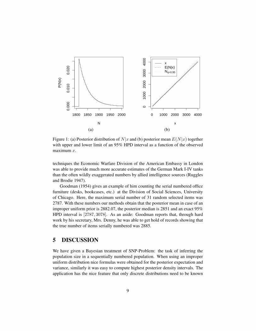
Figure 1 shows in (a) the posterior distribution of N |x. Note the characteristicshape of the shifted factorial distribution: values below x are zero, the mode is at xand the probabilities are strictly decreasing after x. Part (b) of the figure shows theposterior mean E(N |x) and a 95% HPD as a function of the observed maximumx. Here, the linearity in x becomes obvious.

The above estimations and the study of historic sources lead Gráda (2001) tothe conclusion that the collapse of the Muster Bank was caused by a combinationof over-generous credit, insider lending and plain fraud. Therefore, the Bank ofIreland did fulfill its responsibility by not reacting.

Another example of the SNP-Problem is the study of production numbers andcapacity of an industrial production. For example a commercial company mightbe interested in assessing relevant numbers of a competitor. An example of thisis the study of German production numbers during World War II: Using statistical

8

1800 1850 1900 1950 2000

0.00

00.

010

0.02

0

N

P(N

|x)

0 1000 2000 3000 4000

010

0020

0030

0040

00

x

xE(N|x)Nq=0.95

(a) (b)

Figure 1: (a) Posterior distribution of N |x and (b) posterior mean E(N |x) togetherwith upper and lower limit of an 95% HPD interval as a function of the observedmaximum x.

techniques the Economic Warfare Division of the American Embassy in Londonwas able to provide much more accurate estimates of the German Mark I-IV tanksthan the often wildly exaggerated numbers by allied intelligence sources (Rugglesand Brodie 1947).

Goodman (1954) gives an example of him counting the serial numbered officefurniture (desks, bookcases, etc.) at the Division of Social Sciences, Universityof Chicago. Here, the maximum serial number of 31 random selected items was2787. With these numbers our methods obtain that the posterior mean in case of animproper uniform prior is 2882.07, the posterior median is 2851 and an exact 95%HPD interval is [2787, 3078]. As an aside: Goodman reports that, through hardwork by his secretary, Mrs. Denny, he was able to get hold of records showing thatthe true number of items serially numbered was 2885.

5 DISCUSSION

We have given a Bayesian treatment of SNP-Problem: the task of inferring thepopulation size in a sequentially numbered population. When using an improperuniform distribution nice formulas were obtained for the posterior expectation andvariance, similarly it was easy to compute highest posterior density intervals. Theapplication has the nice feature that only discrete distributions need to be known

9

while still making allowance for a full Bayesian treatment of an estimation prob-lem. The SNP-problem offers many opportunities for letting the students per-form their own derivations and experiments. On the page http://www.stat.

uni-muenchen.de/~hoehle/software/bayespopsize/ a selection of R andMaple source code can be found which might provide inspiration.

For the more involved priors the resulting equations are not as nice as for theimproper prior. For example, if a proper uniform prior is used on the interval1, . . . , k the posterior together with its mean and variance are available in closedform expression through the use of Gosper’s algorithm (Wolfram Research 2004a).The above mentioned Maple code contains the necessary derivations.

In case of a negative binomial prior with mean r(1− p)/p and variance r(1−p)/p2 the posterior, its mean and variance can also be derived using hypergeometricfunctions. We only state the posterior distribution and refer to the Maple code forfurther information.

P (N |x) =

(N+r−1

r−1

)(xn

)(1− p)N−x(

Nn

)(x+r−1

r−1

)3F2

[1, 1 + x− n, x + r; 1 + x, 1 + x; 1− p

]Returning to the example of the Munster Bank, assume that one of the former

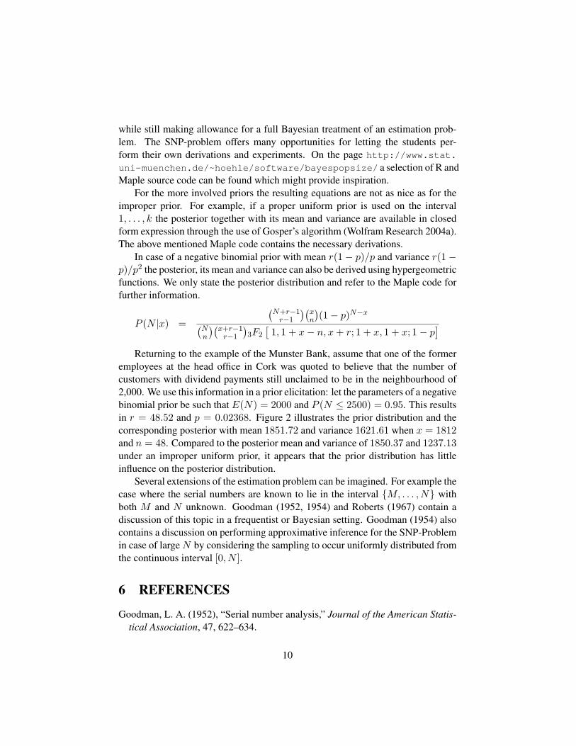
employees at the head office in Cork was quoted to believe that the number ofcustomers with dividend payments still unclaimed to be in the neighbourhood of2,000. We use this information in a prior elicitation: let the parameters of a negativebinomial prior be such that E(N) = 2000 and P (N ≤ 2500) = 0.95. This resultsin r = 48.52 and p = 0.02368. Figure 2 illustrates the prior distribution and thecorresponding posterior with mean 1851.72 and variance 1621.61 when x = 1812and n = 48. Compared to the posterior mean and variance of 1850.37 and 1237.13under an improper uniform prior, it appears that the prior distribution has littleinfluence on the posterior distribution.

Several extensions of the estimation problem can be imagined. For example thecase where the serial numbers are known to lie in the interval {M, . . . , N} withboth M and N unknown. Goodman (1952, 1954) and Roberts (1967) contain adiscussion of this topic in a frequentist or Bayesian setting. Goodman (1954) alsocontains a discussion on performing approximative inference for the SNP-Problemin case of large N by considering the sampling to occur uniformly distributed fromthe continuous interval [0, N ].

6 REFERENCES

Goodman, L. A. (1952), “Serial number analysis,” Journal of the American Statis-tical Association, 47, 622–634.

10

0 1000 2000 3000

0.00

00.

010

0.02

0

N

PriorPosterior

Figure 2: Elicitated negative binomial prior and corresponding posterior distribu-tion in the Munster Bank example.

Goodman, L. A. (1954), “Some Practical Techniques in Serial Number Analysis,”Journal of the American Statistical Association, 49, 97–112.

Gráda, C. O. (2001), “Should the Munster Bank have been saved?” Tech. Rep.WP01/15, Department of Economics, University of Dublin.

Gum, B., Lipton, R., LaPaugh, A., and Fich, F. (2000), “Estimating the maximum,”in Proceedings of the Tenth SIAM Conference on Discrete Mathematics.

Johnson, R. (1994), “Estimating the size of a population,” Teaching Statistics, 16,50–52.

MapleSoft (2004), “Maple v9.5,” http://www.maplesoft.com/products/maple/.

Marlow, W. (1965), “Factorial Distributions,” The Annals of Mathematical Statis-tics, 36, 1066–1068.

Matthews, R. (1998), “Hidden truths,” New Scientist, 158, 28.

R Development Core Team (2006), R: A Language and Environment for StatisticalComputing, R Foundation for Statistical Computing, Vienna, Austria, ISBN 3-900051-07-0.

Roberts, H. V. (1967), “Informative Stopping Rules and Inferences about Popula-tion Size,” Journal of the American Statistical Association, 62, 763–775.

11

Ruggles, R. and Brodie, H. (1947), “An empirical approach to economic intelli-gence in World War II,” Journal of the American Statistical Association, 42,72–91.

Wolfram Research (2004a), “Gosper’s Algorithm,” http://mathworld.wolfram.com/HypergeometricDifferentialEquation.html.

— (2004b), “Hypergeometric Differential Equation,” http://mathworld.wolfram.com/HypergeometricDifferentialEquation.html.

— (2004c), “Stirling Number of the First Kind,” http://mathworld.wolfram.com/StirlingNumberoftheFirstKind.html.

12