bayesian dynamic factor models and portfolio...

Bayesian Dynamic Factor Models and Portfolio

Allocation

Omar AGUILAR and Mike WEST

We discuss the development of dynamic factor models for multivariate financial time series,and the incorporation of stochastic volatility components for latent factor processes. Bayesianinference and computation is developed and explored in a study of the dynamic factor structureof daily spot exchange rates for a selection of international currencies. The models are directgeneralisations of univariate stochastic volatility models, and represent specific varieties of modelsrecently discussed in the growing multivariate stochastic volatility literature. We discuss modelfitting based on retrospective data and sequential analysis for forward filtering and short-termforecasting. Analyses are compared with results from the much simpler method of dynamicvariance matrix discounting that, for over a decade, has been a standard approach in appliedfinancial econometrics. We study these models in analysis, forecasting and sequential portfolioallocation for a selected set of international exchange rate return time series. Our goals are tounderstand a range of modelling questions arising in using these factor models, and to exploreempirical performance in portfolio construction relative to discount approaches. We report on ourexperiences and conclude with comments about the practical utility of structured factor models,and on future potential model extensions.

KEY WORDS: Dynamic Factor Analysis; Dynamic Linear Models; Exchange Rates Forecast-ing; Markov Chain Monte Carlo; Multivariate Stochastic Volatility; PortfolioSelection; Sequential Forecasting; Variance Matrix Discounting

1. INTRODUCTION

Since the mid-1980s, multivariate stochastic volatilitymodels based on variance/covariance discounting (Quin-tana and West 1987, 88) have been used as components ofapplied Bayesian forecasting models in financial economet-ric settings (Quintana 1992; Putnam and Quintana 1994,1995; Quintana and Putnam 1996; Quintana, Chopra andPutnam 1995). The success of such methods in portfo-lio construction is evidenced partly by the fact that theyhave been adopted and are in vigorous day-to-day use ascomponents of global portfolio approaches in several ma-jor international banks. In more recent years, major de-velopments in structured stochastic volatility (SV) mod-elling have led to the introduction of various approachesto modelling dependencies in volatility processes that, inprinciple, may lead to improvements in short-term fore-casting of multiple financial and econometric time series.There is no doubt that these more complex SV modelstheoretically improve the description of several kinds offinancial time series data, including exchange rate returnseries, and hold potential for improvements in practicalshort-term forecasting relative to discount models. Partof our interest here is to empirically explore this poten-tial. We develop dynamic factor, multivariate stochasticvolatility models to address:

Mike West is the Arts and Sciences Professor of Statistics and Deci-sion Sciences, and Director of the Institute of Statistics and DecisionSciences, at Duke University. The address is ISDS, Duke Univer-sity, Durham, NC 27708-0251, USA, and the web site address ishttp://www.stat.duke.edu. Omar Aguilar is Vice President, Mer-rill Lynch Quantitative Research, Merrill Lynch, Mexico City. Thisresearch was partially supported by the National Science Founda-tion under grants DMS 9704432 and 9707914, and by CDC Invest-ment Management Corporation, New York. The authors acknowl-edge useful discussions with Jose M Quintana, Neil Shephard andHong Chang, and the comments and editorial efforts of the JBESEditor. This article is available in electronic form on the ISDS website, http://www.stat.duke.edu

• questions about their potential to provide practicalimprovements in short-term forecasting, and result-ing dynamic portfolio allocations, of international ex-change rates and other financial time series;

• issues of model structuring, implementation, Bayesiananalysis and computation; and

• questions of comparison with the much simpler meth-ods based on variance/covariance discounting.

We study these issues in connection with data analysis andportfolio construction using multiple series of returns oninternational exchange rates.

Variants of the basic method of variance matrix dis-counting (see above references to Quintana and coauthors)have formal theoretical bases in matrix-variate “randomwalks” (Uhlig 1994, 97). Further discussion is given below,and more background can be found in West and Harri-son (1997, section 16.4.5). The basic discounting methodsfollow foundational developments for univariate series inAmeen and Harrison (1985) and Harrison and West (1987),and the formal multivariate models are direct generalisa-tions of univariate models of Shephard (1994a). Relateddiscussion appears in West and Harrison (1997, section10.8.2). In the general multivariate context, the approachleads to the embedding of smoothed estimates of “local”variance/covariance structure within a Bayesian modellingframework, and so provides for adaptation to stochasticchanges as time series data are processed. Modificationsto allow for changes in discount rates in order to adaptto varying degrees of change, including marked/abruptchanges in volatility patterns, extend the basic approach.The resulting update equations for sequences of estimatedvolatility matrices have univariate components that relate

c© ??? American Statistical AssociationJournal of Business & Economic Statistics

???

1

2 Journal of Business & Economic Statistics, ??? ???

closely to variants of ARCH and SV models, and so it isnot surprising that they have proven useful in many appli-cations. However, unlike these more formal models, dis-counting methods do not have real predictive capabilities,simply allowing for and estimating changes rather thananticipating them. Hence the interest in factor modelsthat set out to explicitly describe changes through patternsof time-variation in parameters driving underlying latentprocesses. This is the key motivating concept underlyinginterest in SV models generally, and led has to variousauthors mentioning or developing multivariate SV modelswith dynamic factor structure. Key references include theinitiating work of Harvey, Ruiz and Shephard (1994), andthe later developments in the papers of Jacquier, Polsonand Rossi (1994, 95), and Kim, Shephard and Chib (1998).Several authors have begun to develop and explore relatedfactor models with ARCH/GARCH structure, as opposedto SV structure (e.g., Demos and Sentana 1998). Thoughwe do not discuss this further here, some of the connec-tions and comparisons with SV approaches are of generalinterest, as discussed particularly in the above referencedpaper by Kim et al, and further work on comparative stud-ies might be very worthwhile.

In the following section we detail the basic frameworkand notation for stochastic, time-varying variance matri-ces, followed by discussion of factor structure. We buildon prior work in non-dynamic Bayesian factor analysis anddevelop MCMC methods of model fitting and computa-tion in the chosen class of dynamic factor models. Thesemodels are essentially similar to those introduced in Har-vey, Ruiz and Shephard (1994) and adopted by Jacquier,Polson and Rossi (1994, 95). Our empirical study alsoimplements approximations to sequential analysis and up-dating using the particle filtering methods of Pitt andShephard (1999a). We note that the work reported herewas developed independently of, and in parallel to, thatreported in Pitt and Shephard (1999b), and bears heav-ily on the technical and modelling contributions of thoseauthors. Our computational approaches in model fittingdiffer somewhat from these authors, however. Further-more, our perspective and objectives are fundamentallyon questions of forecasting and portfolio decisions ratherthan exclusively methodological. This is reflected in ourdetailed analyses of international exchange rate time se-ries that discuss model selection and specification, reportson our practical experiences with these models, and makescomparisons with variance discount approaches in analy-sis, forecasting and portfolio construction. We concludewith summary comments and pointers to future work.

2. TIME-VARYING VARIANCE MATRICES AND

FACTOR STRUCTURE

2.1 Introduction and Notation

To introduce notation, consider a q−variate time seriesyt, (t = 1, 2, . . . , ) as conditionally independent, Gaussianrandom vectors with means θt and variance matrices Σt,denoted by N(yt|θt,Σt) for each t. Throughout, our nota-

tion implicitly identifies the conditioning information: forany information set H, p(yt|H) is the conditional densityof yt when H is known. Hence p(yt|θt,Σt) is the condi-tional density of yt when the time t parameters (θt,Σt) areknown, and, implicitly, yt is conditionally independent ofall other relevant quantities when (θt,Σt) are given. Sim-ilarly, if Dt represents all historical data and informationavailable at any time t, then p(yt|Dt−1) is the conditionaldensity of the one-step ahead predictive distribution attime t−1, when all uncertain quantities, usually includingthe parameters (θt,Σt), have been integrated out with re-spect to the relevant posterior distribution conditional onDt−1. This is standard notation in the Bayesian statisticsliterature (e.g., West and Harrison 1997).

Though much applied interest resides in models withsmall time-variations in levels θt predicted via dynamic re-gressions, we adopt a constant level model, θt = θ for all t,for our studies here. A primary interest here is in compar-isons with discount methods in short-term forecasting, sothat the same assumption will be made in discount modelapproaches. Our more recent research and studies in ap-plication have extended the framework to involve dynamicregression components in θt, and through these studies wehave verified that, for the primary goal here of compar-isons with discount methods, the restriction to a constantlevel here is immaterial.

Variance matrix discounting models produce sequencesof posterior distributions for the matrices Σt. Some de-tails are provided in Appendix A, below. The analyses arenaturally sequential, so that posterior distributions are re-vised, or updated, as more data is processed. By way ofnotation, we denote by St the resulting posterior estimateof Σt based on data up to time t, and by St,n the re-sulting posterior estimate of Σt based on the larger setof data up to a time n > t. Live analysis is generally se-quential, with the “current” posterior for Σt at time t ofkey relevance in short-term forecasting; hence the inter-est in point estimates St as they are sequentially updated.Model exploration and development, on the other hand,involves retrospective data analysis; hence the interest inretrospectively revised point estimates St,n.

2.2 Component and Factor Structure

From very early examples and applications of variancematrix discounting, principal component analyses of esti-mated sequences of Σt matrices have been used to explorethe nature of changes over time in covariance patterns,and to provide insight into the latent mechanisms drivingsuch changes. See, for example, the studies of monthlyexchange rate time series in Quintana and West (1987),also reported in West and Harrison (1997, section 16.4.6),where the patterns of change over time in the principalcomponent structure of the estimates St,n are explored. Astandard principal component decomposition of St,n pro-vides insight into the related decomposition of Σt. Often,as in the above examples, this will yield a small numberof dominant components representing latent factors con-tributing measurably to both total variability in the se-ries and the covariance structure, together with additional

Aguilar and West: Bayesian Dynamic Factor Models 3

residual components. This partly underlies the interest indynamic factor models to more explicitly represent the la-tent structure and put the spot-light on inference on fac-tor processes and their parameters. In line with Pressand Shigemasu (1989), Jacquier, Polson and Rossi (1994),Kim, Shephard and Chib (1998), and (extrapolating tothe stochastic volatility context here) Geweke and Zhou(1996), a basic k−factor dynamic model (with k < q,) forΣt is

Σt = XtHtX′

t + Ψt =k

∑

j=1

xtjx′

tjhtj + Ψt (1)

where

• Xt is the q× k factor loadings matrix at time t, withcolumns xtj ,

• Ht = diag(ht1, . . . , htk) is the diagonal matrix of in-stantaneous factor variances, and

• Ψt = diag(ψt1, . . . , ψtq) is the diagonal matrix ofinstantaneous, series-specific or “idiosyncratic” vari-ances.

In terms of the time series yt this is equivalent to therepresentation

yt = θt + Xtft + εt (2)

where

• ft ∼ N(ft|0,Ht) are conditionally independent reali-sations of the k−vector latent factor process,

• εt ∼ N(εt|0,Ψt) are conditionally independent andseries-specific quantities, and

• εt and fs are mutually independent for all t, s.

This is the basic structure we adopt for the rest of thepaper. Our analyses are based on choosing a specific num-ber of factors k throughout. Discussion of choice of k val-ues, and broader related issues of model uncertainty andspecification, follow in section 2.5 and 6. First, we discussfurther structure on the basic factor model with k fixed,and the stochastic volatility components for the factor andidiosyncratic variances.

2.3 Factor Model Constraints

The models analysed and applied in the studies ofthis paper are based on constant factor loadings, so thatXt = X for all t. This provides a framework very similar tothose mooted by the earlier authors, as referenced above,in which we aim to investigate the issues and difficultiesin model implementation.

The k−factor model must be further constrained todefine a unique model free from identification problems.A first constraint is that X be of full rank k to avoididentification problems arising through invariance of themodel under location shifts of the factor loading matrix(e.g., Geweke and Singleton, 1980). Second, we must fur-ther constrain the factor loading matrix to avoid over-parametrisation – simply ensuring that the number of free

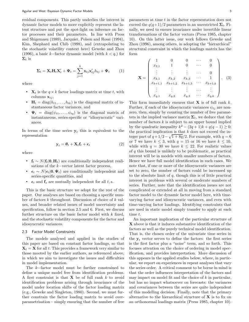
parameters at time t in the factor representation does notexceed the q(q+1)/2 parameters in an unrestricted Σt. Fi-nally, we need to ensure invariance under invertible lineartransformations of the factor vectors (Press 1985, chapter10). On this latter issue, our work follows Geweke andZhou (1996), among others, in adopting the “hierarchical”structural constraint in which the loadings matrix has theform

X =

1 0 0 · · · 0x2,1 1 0 · · · 0

......

... · · · 0xk,1 xk,2 xk,3 · · · 1xk+1,1 xk+1,2 xk+1,3 · · · xk+1,k

......

... · · ·...

xq,1 xq,2 xq,3 · · · xq,k

. (3)

This form immediately ensures that X is of full rank k.Further, if each of the idiosyncratic variances ψtj are non-zero, then, simply by counting the number of free parame-ters in the implied variance matrix Σt, we deduce that thenumber of factors k is subject to an upper bound impliedby the quadratic inequality k2 − (2q + 1)k + q(q − 1) ≥ 0;the practical implication is that k does not exceed the in-teger part of q+1/2−√

1 + 8q/2. For example, with q = 6or 7 we have k ≤ 3, with q = 15 or 16 we have k ≤ 10,while with q = 30 we have k ≤ 22. For realistic valuesof q this bound is unlikely to be problematic, as practicalinterest will be in models with smaller numbers of factors.Hence we have full model identification in such cases. Wenote that, if one or more of the idiosyncratic variances areset to zero, the number of factors could be increased upto the absolute limit of q, though this is of little practicalinterest in problems with several or moderate numbers ofseries. Further, note that the identification issues are notcomplicated or extended at all in moving from a standardfactor model to the dynamic factor model here, with time-varying factor and idiosyncratic variances, and even withtime-varying factor loadings. Identifying constraints thatare used in static model simply transfer to apply at eachtime t.

An important implication of the particular structure ofX above is that it induces substantive identification of thefactors as well as the purely technical model identification.That is, the chosen order of the univariate time series inthe yt vector serves to define the factors: the first seriesis the first factor plus a “noise” term, and so forth. Thisfocuses attention on the choice of ordering in model spec-ification, and provides interpretation. More discussion ofthis appears in the applied studies below, where, in partic-ular, we report on experiences in repeat analyses that varythe series order. A critical comment to be borne in mind isthat the order influences interpretation of the factors andmay impact on model fit and the choice of k in particular,but has no impact whatsoever on forecasts: the variancesand covariances between the series are quite independentof this modelling decision. Finally, note that the primaryalternative to the hierarchical structure of X is to fix onan orthonormal loadings matrix (Press 1985, chapter 10).


We very much prefer the hierarchical structure primarilyfor the reasons of substantive interpretation of the factors,just discussed, and also as the resulting Bayesian analysisis much less technically complicated.

2.4 Stochastic Volatility Model Components

Multivariate generalisations of univariate SV modelsthrough dynamic factor models are mentioned by vari-ous authors, including Harvey, Ruiz and Shephard (1994),Shephard (1996), Kim, Shephard and Chib (1998), andhave been investigated by Jacquier, Polson and Rossi(1995). The basic model of the latter authors assumesthat the univariate factor series fti follow standard uni-variate SV models, but discuss possible extensions alsomentioned in Kim, Shephard and Chib (1998). We adoptsuch an extension here, one in which the log volatilities ofthe factors follows a vector autoregression with correlatedinnovations, an extension that turns out to be of relevancein studies of exchange rate returns. We additionally adoptunrelated, univariate stochastic volatility models for theidiosyncratic variances.

For the factor variances, define λti = log(hti) foreach i = 1, . . . , k and write λt = (λt1, . . . , λtk)′. Weassume a stationary vector autoregression of order one,VAR(1), centered around a mean µ = (µ1, . . . , µk)

′

andwith individual AR parameters φi in the matrix Φ =diag(φ1, . . . , φk). That is, for t = 1, 2 . . . , we have

λt = µ + Φ(λt−1 − µ) + ωt (4)

with independent innovations

ωt ∼ N(ωt|0,U) (5)

for some innovations variance matrix U. The impliedmarginal distribution for each λt is then

λt ∼ N(λt|µ,W) (6)

where W satisfies W = ΦWΦ + U and has elementsWij = Uij/((1−φi)(1−φj)). The model allows dependen-cies across volatility series through non-zero off-diagonalentries in U and W. Also, this marginal distribution de-fines the initial distribution for λ0.

For the idiosyncratic variances, define ηtj = log(ψtj)for each j = 1, . . . , q. For these series of log variances weassume standard univariate autoregressions of order one,namely

ηtj = αj + ρj(ηt−1,j − αj) + ξtj

with independent innovations ξtj ∼ N(ξtj |0, sj). Unlikethe factor volatilities, the ηtj processes are mutually inde-pendent series. Write α = (α1, . . . , αq), ρ = (ρ1, . . . , ρq)and s = (s1, . . . , sq) for the vectors of parameters here.Our models assume stationarity and positive dependencewithin each series, so that 0 < ρj < 1 for each j andthe implied stationary marginal distributions are given byN(ηtj |αj , sj/(1 − ρ2

j )), including the case t = 0 that pro-vides the initial priors for the volatility series.

2.5 Model Specification and Practical Perspectives

Our discussion of model fitting and analyses, and appli-cations below, are based on specific k−factor models. Wedo discuss some empirical experiences with varying thevalue of k in our exchange rate studies, though do not for-mally address inference on k here. In this connection, somegeneral points to note are as follows. First, in analysingdata consistent with a factor structure but with a model inwhich k is too large, we should expect to see multimodali-ties appearing in posterior densities for the elements of thefactor loading matrix (Geweke and Singleton 1980; Lopesand West 1998). As illustrated in the latter reference, wehave experienced this in standard (non-dynamic) factormodels and the idea translates directly. Experiencing thiswould suggest that k be decreased. Second, and relatedto this, approaches to analysis using MCMC will tend toexperience convergence difficulties in models with k toolarge; this has also been verified in ranges of studies ofour exchange rate series with these dynamic factor mod-els, as we discuss in the application sections below. Bycontrast, in a model in which k appears to be appropri-ate for the data under study, our experiences are that theMCMC algorithms converge rapidly and cleanly, again asin standard, non-dynamic factor models.

The broader question of inference on k is interestingand challenging. In Lopes and West (1998) we have ex-plored a range of approaches to inference on k, Bayesianand likelihood-based. Translating this to the dynamic fac-tor context is as yet unexplored.

From a serious practical viewpoint, we here outline whathas been a useful exploratory perspective on choosing k –or a range of possible values of k to explore in parallel –in our applied work. In our studies of the exchange rateseries we are interested in sequential forecasting and port-folio, and have a wealth of historical data at hand to use inmodel construction and the exploratory phases of analysis.Our examples below are founded on such an explorationof an initial stretch of historical data, followed by formalmodel fitting to the remaining data. In line with this, wechoose both the value, or values, of k and hyperparame-ters of informative prior distributions for model parame-ters based on a rather informal look at some such initialdata. A referee has referred to this as “ad hoc”, and tosome extent it is. It is also a scientifically sensible, permis-sible and practicable approach to initial model and priorspecification, and perfectly formal and coherent from theviewpoints of statistical inference. In the exchange ratestudies, we have a series of over 1,827 daily observationsat hand. From an exploratory analysis of just the first200 days, we settle on choices of k and prior distributionsfor the model to be used from that time point onward,fitting the so-specified model to the remaining data. Inthis initial analysis phase, we explore the early stretch ofdata using the variance matrix discounting method. Thisis simple, robust and trivially implemented to produce es-timated sequences of Σt matrices over this first short sec-tion of historical data. As exemplified in various previousstudies (e.g., Quintana and West 1987; West and Harrison


1997, chapter 16) using principal component decomposi-tions of these sequences, such analysis provides insight intothe underlying factor structure. In our current work, weuse Cholesky decompositions of the estimated Σt matricesrather than principal components. The Cholesky decom-positions map directly onto the factor model form of thispaper, and so provides direct insight into plausible rangesof values for factor model parameters, including k, thatcan be used to develop informed (though still very diffuse)priors to feed into the formal analysis of the remainingdata. This strategy is used below, where more details aregiven of the specific experiences with our chosen exchangerate series.

To be explicit technically, note that the Cholesky decom-position is Σt = LtL

′

t where Lt is a q × q lower triangularmatrix with non-negative diagonal elements (all positive ifΣt is of full rank). This can be expressed as Σt = XtHtX

′

t

with Lt = XtHt1/2 where the q× q matrix Xt is lower tri-

angular with diagonal elements of unity, and Ht is a q× qdiagonal matrix whose diagonal elements are the squaresof those of Lt. Thus we have a full factor representationwith k = q and zero idiosyncratic variances. Assuming arestricted factor model with k < q is appropriate, we sim-ply identify the k largest values of Ht as the conditionalvariances of the k factors, and the first k columns of Xt

as the corresponding factor loading matrix; then addingnon-zero idiosyncratic variances provides a k−factor ap-proximation.

3. BAYESIAN INFERENCE AND COMPUTATION

3.1 MCMC analysis

The model as specified so far comprises the basic fac-tor structure (2) with supporting assumptions, specialisedto fixed parameters θt = θ and Xt = X, and incorporat-ing the SV models of Section 2.4. Model completion forBayesian analysis requires prior distributions for the fullset of parameters {θ,X; µ,Φ,U; α,ρ, s}. Bayesian infer-ence for any specified prior requires the computation andsummarisation of the implied posteriors for these modelparameters, together with inferences on the factor pro-cesses ft and the log-volatility sequences λt and ηtj (foreach j = 1, . . . , q), over the time window of t = 1, 2, . . . , nconsecutive observations comprising the information setDn. Computation via MCMC simulation builds on boththe work of previous authors in the SV and factor mod-elling literature, and previous work by the current authorsin quite different models with related technical structure(Aguilar and West 1998; West and Aguilar 1997).

To complete the model specification, we assume a priorspecified in terms of conditionally independent compo-nents

p(θ)p(X)p(µ)p(Φ)p(U)p(α)p(ρ)p(s) (7)

where the chosen marginal priors are either standard ref-erence priors or proper priors that are chosen to be condi-tionally conjugate, as discussed below. The outlook hereis to explore the use of reference priors to the extent pos-

sible to provide an initial analysis framework. Our priorspecifications reflect this view, though, as discussed above,we do use relatively diffuse though proper priors for somemodel components. Further, specific applications may usealternative prior specifications, both in terms of informa-tive priors on model components and in terms of prior de-pendencies between parameters, though we do not discussother prior specifications here.

First, we assume standard reference priors for the uni-variate entries in the conditional mean θ and the factorloading matrix X, so that p(θ)p(X) ∝ constant. Note thatthe prior for X is, of course, subject to the specified 0/1constraints on values in the the upper triangle and diago-nal in (3), so the constant prior density applies only to theremaining, uncertain elements. Second, we use indepen-dent normal priors for the univariate elements of µ,α, thediagonal elements of Φ and the elements of ρ. This allowsfor both reference priors, by setting the prior precisionsto zero, and restriction of the values of each φj and ρj byadapting the prior to be truncated to (0, 1). Third, we usean informative inverse Wishart prior for the VAR(1) inno-vations variance matrix U in the SV model for the factorvolatilities. This is specified with hyperparameters basedon prior discounting analysis of an initial, reserved sectionof data as discussed above. Notice that an improper ref-erence prior on U, could lead to problems as U and Ψt

determine two separate sources of variability in the datathat are confounded in the model. This point, rather crit-ical to model implementation and resulting data analysis,is almost implicit in the prior work of Kim, Shephard andChib (1998). These authors use informative proper priorsfor innovations variances that parallel our assumptions intheir univariate SV models; though they present these pri-ors without further discussion, the propriety is critical inovercoming otherwise potentially problematic confound-ing issues. Hence initial analysis of previous data, or someother prior elicitation activity, is needed. As mentionedabove, our applied development uses variance discount-ing analyses in providing easy preliminary analysis of areserved initial section of data as input to this. Thoughsomewhat secondary, the fact that we choose to summarisethis prior information in terms of a prior for U of condi-tionally conjugate inverse Wishart form does help in thefollowing MCMC analysis of the factor model. Finally, weuse a similar idea and strategy in specifying diffuse thoughproper inverse gamma priors for the elements of s, assum-ing conditional independence across series.

Iterative posterior simulation uses an MCMC strategythat extends those in existing SV models (Jacquier, Pol-son and Rossi 1995; Kim, Shephard and Chib 1998) tothe multivariate case, introduces elements of MCMC algo-rithms for Bayesian factor analysis as in Geweke and Zhou(1996), and adds novel components derived from modelswith latent VAR components developed by the current au-thors in a quite different context (Aguilar and West 1998;West and Aguilar 1997). We iteratively simulate valuesof all model parameters together with the full set of val-ues of the latent processes ft,λt and the ηtj by sequenc-ing through the set of conditional distributions detailed in


Appendix B. At some stages we have direct conditionalsimulations, at others we require the introduction of novelMetropolis-Hastings accept/reject steps. We note in pass-ing that, from an algorithmic viewpoint, there are variouspossible extensions and alternative methods for compo-nents of the MCMC analysis, such as in utilising someof the ideas from Shephard and Pitt (1997) for exam-ple, though we have not explored such variants yet. Wenote that Pitt and Shephard (1999b) explore similar factormodels and alternative computational schemes for modelfitting and sequential analysis; our work was developed in-dependently of, and in parallel to, that study, and somefuture comparisons of numerical methods will be of inter-est. Beyond the appendix material here, further technicaldetails are available on request from the authors.

3.2 Sequential Filtering

Recent work in sequential methods of Bayesian anal-ysis using simulation-based approaches has contributedsignificant methodology of use in broad classes of mod-els, especially for problems of sequential learning on time-varying state parameters such as the stochastic volatilitymatrix Ht in our factor models. There is much currentresearch concerned with developing such methods, whichgo back at least to West (1993) in the statistics litera-ture, though they are not yet general enough to adequatelyhandle larger scale problems that, in addition to evolvingstates, have several or many fixed model parameters. Si-multaneous sequential inference on the factor model pa-rameters {θ,X; µ,Φ,U; α,ρ, s} as well as all the time-evolving volatility processes {Ht,Ψt} is an open researchproblem. For this reason, our current study explores se-quential forecasting and portfolio allocations for a longsection of the time series, based on chosen estimates ofall fixed model parameters. The parameter estimates aretaken from the MCMC analysis of a prior stretch of his-torical data. The strategy, which is “honest” from theviewpoint of sequential forecasting, is illustrated in theapplication to exchange rates below.

The sequential filtering methods adopted for updatingposteriors on the time-evolving volatility processes arebased on the auxiliary particle filtering (APF) method ofPitt and Shephard (1999a). The APF method is a proventechnique for sequential updating of simulation-based sum-maries of posterior distributions for time-evolving states,and at each time t delivers a current sample of points fromthe prior p(Ht,Ψt|Dt−1) and then the resulting poste-rior p(Ht,Ψt|Dt). These samples are trivially mapped intosimilar samples from the corresponding prior p(Σt|Dt−1)and posterior p(Σt|Dt) by direct computation using Σt =XHtX

′ + Ψt where X is estimated as just discussed. Forportfolio allocations in this framework we require the one-step ahead forecast means and variance matrices of thereturns, namely gt = E(yt|Dt−1) and Gt = V (yt|Dt−1)at time t − 1. These are easily evaluated. The mean gt

is constant, gt = g, simply the estimate of θ previouslycomputed from the analysis of the initial data segment.

The forecast variance Gt is computed as the sample meanof the Monte Carlo sample of variance matrices Σt repre-senting p(Σt|Dt−1).

We note and stress that, although this analysis ignoresthe fact that the model parameters are fixed over thecourse of the sequential portfolio allocation part of thestudy, the analysis nevertheless provides a coherent ba-sis for model comparisons with a utility function directlymeasuring real-world performance in terms of cumulativefinancial returns. Any advances in statistical methods toadequately incorporate learning about the fixed model pa-rameters together with the volatilities in the sequentialcontext will only improve matters. Further discussion ofthis, and other practical issues and experiences, appear inthe exchange rate studies below. Additional support forthe efficacy of the APF method in factor models is given inPitt and Shephard (1999b). More recent developments ofthis method, that extend the particle filtering techniquesto incorporate fixed model parameters, are discussed inLiu and West (2000), with studies of their efficacy in thisclass of dynamic factor models.

4. STUDIES OF INTERNATIONAL EXCHANGE RATES

4.1 Data and Initial Discounting Analyses

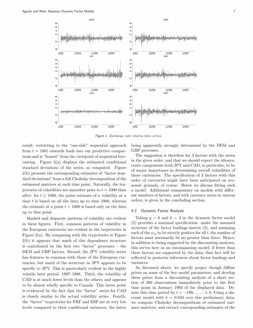
Figure 1 displays time series graphs of the returns onweekday closing spot rates for several currencies relativeto the US dollar during the period from January 1st, 1992to December 31st 1998, with a total of 1827 data pointsin each series. The currencies are, in order, the Ger-man Mark (DEM), British Pound (GBP), Japanese Yen(JPY), French Franc (FRF), Canadian Dollar (CAD) andSpanish Peseta (ESP). The series were obtained from datavendor DataStream. We analyse the one-day-ahead re-turns as graphed, namely yti = sti/st−1,i − 1 for currencyi = 1, . . . , q = 6. In some of the graphs we have markedthe point t = 1000, corresponding to October 31st, 1995,as a reference. We now discuss and summarise retrospec-tive model analyses of the data prior to this time point,followed by studies of sequential updating analyses andout-of-sample forecasting beyond this time point. The se-ries are ordered in the yt vectors as listed above.

Initial exploratory analysis using variance matrix dis-counting with the controlling discount factor set at δ =0.942 is summarised in Figures 2. This analysis was chosenfollowing a set of parallel analyses differing only throughthe value of δ, with δ values spanning a grid over 0.9 − 1.At each δ value the marginal likelihood function is triv-ially computed from the discount analysis, resulting in afull marginal likelihood function for δ. This chosen value(δ = 0.942) is the resulting MLE from such analyses ofthe first 1000 time points only. In Figures 2 we presentsome point estimates of aspects of the sequence of Σt ma-trices extracted from (a) the smoothed estimates St,1000

over the period up to 10/31/95, i.e., t = 1000, and (b) thesequentially updated estimates St over the period fromthen until the end of the data at 12/31/98. The initialperiod presents smoother estimates than the latter, as a


-6-2

24

68

1/92 12/93 11/95 10/97

DEM

-6-2

24

68

1/92 12/93 11/95 10/97

GBP

-6-2

24

68

1/92 12/93 11/95 10/97

JPY

-6-2

24

68

1/92 12/93 11/95 10/97

FRF-6

-22

46

8

1/92 12/93 11/95 10/97

CAD

-6-2

24

68

1/92 12/93 11/95 10/97

ESP

Figure 1. Exchange rate returns time series.

result; restricting to the “one-side” sequential approach

from t = 1001 onwards leads into our predictive compar-

isons and is “honest” from the viewpoint of sequential fore-

casting. Figure 2(a) displays the estimated conditional

standard deviations of the series, so computed. Figure

2(b) presents the corresponding estimates of “factor stan-

dard deviations” from a full Cholesky decomposition of the

estimated matrices at each time point. Naturally, the tra-

jectories of volatilities are smoother prior to t = 1000 than

after: for t ≤ 1000, the point estimate of a volatility at a

time t is based on all the data up to time 1000, whereas

the estimate at a point t > 1000 is based only on the data

up to that point.

Marked and disparate patterns of volatility are evident

in these figures. First, common patterns of volatility in

the European currencies are evident in the trajectories in

Figure 2(a). By comparing with the trajectories in Figure

2(b) it appears that much of this dependence structure

is contributed by the first two “factor” processes – the

DEM and GBP factors. Second, the JPY volatility series

has features in common with those of the European cur-

rencies, but much of the structure in JPY appears to be

specific to JPY. This is particularly evident in the highly

volatile later period, 1997–1998. Third, the volatility of

CAD is at much lower levels than the others, and appears

to be almost wholly specific to Canada. This latter point

is evidenced by the fact that the “factor” series for CAD

is closely similar to the actual volatility series. Fourth,

the “factor” trajectories for FRF and ESP are at very low

levels compared to their conditional variances, the latter

being apparently strongly determined by the DEM andGBP processes.

The suggestion is therefore for 3 factors with the seriesin the given order, and that we should expect the idiosyn-cratic components both JPY and CAD, in particular, to beof major importance in determining overall volatilities ofthose currencies. The specification of 3 factors with thisorder of currencies might have been anticipated on eco-nomic grounds, of course. Below we discuss fitting sucha model. Additional commentary on models with differ-ent numbers of factors, and with currency series in variousorders, is given in the concluding section.

4.2 Dynamic Factor Analysis

Taking q = 6 and k = 3 in the dynamic factor model(2) provides a maximal specification: under the assumedstructure of the factor loadings matrix (3), and assumingeach of the ψtj to be strictly positive for all t, the number offactors must necessarily be no greater than three. Hence,in addition to being suggested by the discounting analyses,this serves here as an encompassing model; if fewer thanthree factors are supported by the data, that fact will bereflected in posterior inferences about factor loadings andvariances.

As discussed above, we specify proper though diffusepriors on some of the key model parameters, and developthese priors from a discounting analysis of a short sec-tion of 200 observations immediately prior to the firsttime point in January 1992 of the displayed data. De-note this time period by t = −199, . . . ,−1, 0. Using a dis-count model with δ = 0.942 over this preliminary data,we compute Cholesky decompositions of estimated vari-ance matrices, and extract corresponding estimates of the


(a) Conditional standard deviations of returns

0.0

0.01

00.

020

1/92 12/93 11/95 10/97

DEM

0.0

0.01

00.

020

1/92 12/93 11/95 10/97

GBP

0.0

0.01

00.

020

1/92 12/93 11/95 10/97

JPY

0.0

0.01

00.

020

1/92 12/93 11/95 10/97

FRF

0.0

0.01

00.

020

1/92 12/93 11/95 10/97

CAD

0.0

0.01

00.

020

1/92 12/93 11/95 10/97

ESP

(b) Conditional standard deviations of “factors”

0.0

0.01

00.

020

1/92 12/93 11/95 10/97

DEM

0.0

0.01

00.

020

1/92 12/93 11/95 10/97

GBP

0.0

0.01

00.

020

1/92 12/93 11/95 10/97

JPY

0.0

0.01

00.

020

1/92 12/93 11/95 10/97

FRF

0.0

0.01

00.

020

1/92 12/93 11/95 10/97

CAD

0.0

0.01

00.

020

1/92 12/93 11/95 10/97

ESP

Figure 2. (a) Time trajectories of estimated conditional standard deviations of the returns time series from the discount analysis (squareroots of the diagonal element of the estimated Σt sequence.). (b) Corresponding trajectories of the conditional standard deviations of the“factors” underlying the returns time series from the discount analysis (diagonal elements of the Cholesky decomposition of the estimatedΣt sequence).


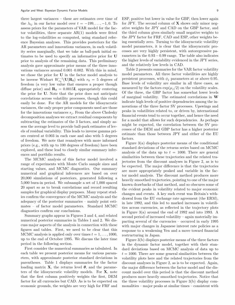
three largest variances – these are estimates over time ofthe λtj in our factor model over t = −199, . . . ,−1, 0. Toassess priors for the parameters of VAR model for the fac-tor volatilities, three separate AR(1) models were fittedto the log-volatilities so computed, using standard refer-ence Bayesian analyses. This provides posteriors for theAR parameters and innovations variances, in each volatil-ity series marginally, that we take as ball-park initial es-timates to be used to specify an informative prior for U

prior to analysis of the remaining data. This preliminaryanalysis gave approximate prior means of the three inno-vations variances around 0.001–0.002. With this in mind,we chose the prior for U in the factor model analysis tobe inverse Wishart W−1

r0(U|R0) with r0 = 5 degrees of

freedom (a very low value that ensures a proper thoughdiffuse prior) and R0 = 0.0015I, appropriately centeringthe prior for U. Note that the prior does not anticipatecorrelations across volatility processes, though this couldeasily be done. For the AR models for the idiosyncraticvariances, the only proper prior components used are thosefor the innovations variances sj . From the above Choleskydecomposition analyses we extract residual components bysubtracting the estimates of the 3 factors, and simply as-sess the average level to provide ball-park estimates of lev-els of residual variability. This leads to inverse gamma pri-ors centred at 0.003 in each case and also with 5 degreesof freedom. We note that reanalyses with more informedpriors (e.g., with up to 100 degrees of freedom) have beenexplored, and these lead to closely similar summary infer-ences and portfolio results.

The MCMC analysis of this factor model involved arange of experiments with Monte Carlo sample sizes andstarting values, and MCMC diagnostics. Our summarynumerical and graphical inferences are based on over20,000 simulations of posteriors, generated following a5,000 burn-in period. We subsample a set of 1,000 spaced20 apart so as to break correlations and record resultingsamples for graphical display purposes. Many repeat stud-ies confirm the convergence of the MCMC analysis and theadequacy of the posterior summaries – mainly point esti-mates – of factor model parameters. Standard MCMCdiagnostics confirm our conclusions.

Summary graphs appear in Figures 3 and 4, and relatednumerical posterior summaries in Tables 1 and 2. We dis-cuss major aspects of the analysis in connection with thesefigures and tables. First, we need to be clear that thisMCMC analysis is applied only over times t = 1, . . . , 1000,up to the end of October 1995. We discuss the later timeperiod in the following section.

First consider the numerical summaries as tabulated. Ineach table we present posterior means for various param-eters, with approximate posterior standard deviations inparentheses. Table 1 displays summaries for the factorloading matrix X, the returns level θ, and the parame-ters of the idiosyncratic volatility models. For X, notethat the first column positively weights the first, DEMfactor for all currencies but CAD. As is to be expected oneconomic grounds, the weights are very high for FRF and

ESP, positive but lower in value for GBP, then lower againfor JPY. The second column of X shows only minor neg-ative weights for JPY and CAD on the GBP factor, andthe third column gives similarly small negative weights tothe JPY factor for FRF, CAD and ESP, other weights be-ing essentially zero. Turning to the idiosyncratic volatilitymodel parameters, it is clear that the idiosyncratic pro-cesses are very highly persistent, with autoregressive pa-rameters in the 0.93−0.99 range. The table also indicatesthe higher levels of variability evidenced in the JPY series,and the relatively low levels in CAD.

Table 2 presents summaries for the VAR factor volatilitymodel parameters. All three factor volatilities are highlypersistent processes, with φj parameters at or above 0.95.Base levels of volatility are similar in all three cases, asmeasured by the factors exp(µj/2) on the volatility scales.Of the three, the GBP factor has somewhat lower levelsof marginal volatility. The estimated correlations in W

indicate high levels of positive dependencies among the in-novations of the three factor SV processes. Upswings andpeaks in volatilities related to, or driven by, internationalfinancial events tend to occur together, and hence the needfor a model that allows for such dependencies. As perhapsmight be expected, the correlation between the SV pro-cesses of the DEM and GBP factor has a higher posteriorestimate than those between JPY and either of the EUfactors.

Figure 3(a) displays posterior means of the conditionalstandard deviations of the returns series based on MCMCanalysis of the data up to t = 1000. There are generalsimilarities between these trajectories and the related tra-jectories from the discount analyses in Figure 2, as is tobe expected. The major difference is that the trajectoriesare more appropriately peaked and variable in the fac-tor model analysis. The discount method produces moreheavily smoothed trajectories, pointing to one of the majorknown drawbacks of that method, and so obscures some ofthe evident peaks in volatility related to major economicchanges and events. A key such event was Britain’s with-drawal from the EU exchange rate agreement (the ERM),in late 1992, and this led to marked increases in volatili-ties across currencies, as reflected in the trajectory plotsin Figure 3(a) around the end of 1992 and into 1993. Asecond period of increased volatility – again materially im-pacting several of the currencies – occurred in early 1995with major changes in Japanese interest rate policies as aresponse to a weakening Yen and a move toward financialrestructuring in Japan.

Figure 3(b) displays posterior means of the three factorsin the dynamic factor model, together with their stan-dard deviations based on MCMC analysis of data up tot = 1000. There are some general similarities between thevolatility plots here and the related trajectories from thediscount analyses in Figure 2, as is to be expected. Again,the major difference between the factor model and the dis-count model over this period is that the discount methodproduces more heavily smoothed trajectories. Notice thatthe three volatility processes in Figure 3(b) display com-monalities – major peaks at similar times – consistent with


(a) Conditional standard deviations of returns

0.00

50.

015

0.02

5

1/92 12/93 11/95 10/97

DEM

0.00

50.

015

0.02

5

1/92 12/93 11/95 10/97

GBP

0.00

50.

015

0.02

5

1/92 12/93 11/95 10/97

JPY

0.00

50.

015

0.02

5

1/92 12/93 11/95 10/97

FRF

0.00

50.

015

0.02

5

1/92 12/93 11/95 10/97

CAD

0.00

50.

015

0.02

5

1/92 12/93 11/95 10/97

ESP

(b) Estimated factors and their standard deviations

-0.0

40.

00.

04

1/92 7/92 2/93 9/93 4/94 1/95 8/95

DEM

0.0

0.01

00.

020

1/92 12/93 11/95 10/97

-0.0

40.

00.

04

1/92 7/92 2/93 9/93 4/94 1/95 8/95

GBP

0.0

0.01

00.

020

1/92 12/93 11/95 10/97

-0.0

40.

00.

04

1/92 7/92 2/93 9/93 4/94 1/95 8/95

JPY

0.0

0.01

00.

020

1/92 12/93 11/95 10/97

Figure 3. (a) Posterior means of the conditional standard deviations of the returns series based on MCMC analysis of the data up tot = 1000, and then based on particle filtering from that point to the end of the time period. (b) Posterior means of the three factors and theirstandard deviations up to t = 1000 based on MCMC analysis of data to that time point. The volatility graphs also include the sequentiallyupdated estimates from t = 1001 based on particle filtering from that point to the end of the time period.


(a) Estimated idiosyncratic standard deviations

0.0

0.01

00.

020

1/92 12/93 11/95 10/97

DEM

0.0

0.01

00.

020

1/92 12/93 11/95 10/97

GBP

0.0

0.01

00.

020

1/92 12/93 11/95 10/97

JPY

0.0

0.01

00.

020

1/92 12/93 11/95 10/97

FRF

0.0

0.01

00.

020

1/92 12/93 11/95 10/97

CAD

0.0

0.01

00.

020

1/92 12/93 11/95 10/97

ESP

(b) Percent variation explained by idiosyncratics

020

4060

80

1/92 12/93 11/95 10/97

DEM

020

4060

80

1/92 12/93 11/95 10/97

GBP

020

4060

80

1/92 12/93 11/95 10/97

JPY

020

4060

80

1/92 12/93 11/95 10/97

FRF

020

4060

80

1/92 12/93 11/95 10/97

CAD

020

4060

80

1/92 12/93 11/95 10/97

ESP

Figure 4. (a) Posterior means of the idiosyncratic standard deviations of the returns series based on MCMC analysis of the data up tot = 1000, and then based on particle filtering from that point to the end of the time period. (b) Percentage variation in the return seriesexplained by the idiosyncratic variances, computed based on posterior means of all variances at each time point. As above, the estimatesare based on MCMC analysis of the data up to t = 1000, and then based on particle filtering from that point to the end of the time period.


Table 1.Posterior means (SDs) for the factor loadings matrix, mean vector and parameters of the idiosyncratic SV models based on MCMCanalysis of data up to 10/31/1995. (All truncated to 2 decimal places, so the zero SD entries indicate values smaller than 0.01.)

Factor loadings matrix X θ (×10−4) ρj eαj/2 (×10−3)√

sj/(1 − ρ2

j )

DEM 1 0 0 −1.50 (1.28) 0.99 (0.00) 0.52 (0.23) 1.45 (0.20)GBP 0.67 (0.03) 1 0 0.17 (0.98) 0.99 (0.00) 0.57 (0.21) 1.54 (0.25)JPY 0.53 (0.02) −0.05 (0.03) 1.00 (0.00) −2.33 (1.18) 0.99 (0.00) 0.74 (0.28) 1.59 (0.38)FRF 0.97 (0.01) −0.00 (0.01) −0.02 (0.01) −1.24 (1.25) 0.98 (0.03) 0.30 (0.24) 1.33 (0.21)CAD −0.03 (0.01) 0.04 (0.02) −0.06 (0.01) −1.23 (0.59) 0.94 (0.01) 0.26 (0.01) 0.68 (0.06)ESP 0.95 (0.01) −0.00 (0.01) −0.02 (0.01) −1.59 (1.26) 0.93 (0.01) 0.20 (0.02) 1.63 (0.12)

Table 2. Posterior means (SDs) for parameters of the factor SV model based on MCMC analysis of data up to 10/31/1995.

φj eµj /2(×10−3) SDs and correlations in W

j = 1 0.95 (0.01) 5.73 (0.32) 0.68 (0.07)j = 2 0.96 (0.01) 3.68 (0.28) 0.52 (0.08) 0.81 (0.08)j = 3 0.96 (0.01) 4.91 (0.37) 0.43 (0.08) 0.45 (0.09) 0.78 (0.09)

the positive dependencies across processes evident in theestimated correlations in the factor SV model.

Figure 4(a) displays posterior means of the idiosyncraticstandard deviations of the returns series based on MCMCanalysis of the data up to t = 1000. One of the key featuresevident here is the fact that the idiosyncratic variance pro-cess for JPY was almost negligible over this period up to1995. Additional features of note are the very low levelsof idiosyncratic variability for DEM and GBP, and, as ex-pected, for CAD. Further, there is significant idiosyncraticvariability in ESP as compared to FRF, reflecting the factthat FRF is more closely tied to the dominant Europeancurrencies, and DEM in particular through the ERM, thanis ESP.

Figure 4(b) displays levels of variation in each of thecurrency return series contributed by their idiosyncraticvariances, computed as percentages of the overall condi-tional variances. The estimates are computed by estimat-ing all variances by their posterior means based on MCMCanalysis of the data up to t = 1000. Of major note here isCAD; the trajectory indicates that volatility fluctuationsin CAD are almost wholly idiosyncratic and unrelated tothe European and Japanese factors.

5. SEQUENTIAL FORECASTING AND PORTFOLIO

ALLOCATIONS

5.1 Perspective

Model comparisons are made with explicit focus on one-step forecast accuracy in the context of dynamic portfolioallocations, essentially following the perspective of Quin-tana (1992), Putnam and Quintana (1994), and Quintanaand Putnam (1996). A similar perspective is adopted inPolson and Tew (1997) though with very different models.Our comparisons in this section are based on sequentialupdating and one-step ahead forecasting, with resultingportfolio allocation decisions implemented one-step ahead.At each time point t − 1, we suppose that an existing in-vestment in the various currencies under study may bereallocated according to a portfolio at for the next time

point. The elements of at are the amounts invested in thecorresponding currency. For this comparative analysis, weassume no transaction costs and that we may freely re-allocate dollars instantaneously to long or short positionsacross the currencies. These allocation decisions are madesequentially; the choice of at is made at time t− 1 basedon the current, one-step ahead predictive distribution foryt conditional on current and past data and informationDt−1. The realised portfolio return at time t is rt = a′

tyt,and models may be compared on the basis of cumulativereturns over chosen time intervals.

Our study involves the general Markowitz mean-variance optimisation, applied at each time point one-stepahead. Thus the utility structures used for portfolio alloca-tions require evaluation and sequential revision of the one-step ahead forecast means and variance matrices of the re-turns, denoted by gt = E(yt|Dt−1) and Gt = V (yt|Dt−1)at time t − 1. Computations in the variance matrix dis-counting analysis are simple and standard: these one-stepahead forecast distributions are multivariate T with eas-ily updated parameters gt and Gt. Sequential computa-tions and updating in dynamic factor models are quitenon-standard, and challenging, and are here based on se-quential methods of updating and generating Monte Carloapproximations to prior and posterior distributions. Thesedeliver sets of samples representing the key distributionsp(Σt|Dt−1), and updates to these samples as t changesand new data are processed. These samples deliver MonteCarlo approximations to the required one-step ahead fore-cast means and variance matrices, and these are used inthe portfolio allocation computations.

5.2 Sequential Analysis and Approximations

As discussed above, we explore sequential forecastingand portfolio allocations from t = 1001 onwards, usingparticle filtering methods to sequential update posteriorsfor volatility processes and so feed into the one-step-aheadportfolio decisions. We have earlier partitioned the dataat time t = 1000, and applied the MCMC analysis to thatinitial time period. From this analysis, we compute theposterior means of all model parameters in the above set,and from that point t = 1000 onwards behave as if these


parameters are all fixed at these estimates. Over the re-maining time interval, a total of 827 days, we then applythe auxiliary particle filtering (APF) method of Pitt andShephard (1999a) to sequentially revise posterior distribu-tions for the volatility processes {Ht,Ψt}. As discussedin subsection 3.2, this easily delivers sequentially updatedMonte Carlo estimates of one-step ahead forecast meansand variance matrices of the returns, gt = E(yt|Dt−1) andGt = V (yt|Dt−1), as required. Recall that we assume aconstant mean for our studies here, so that gt = g, theestimate of θ based on the first 1000 observations.

This use of model parameters at their posterior meanscomputed only on data prior to time t = 1000 leads toextremely interesting results. One such is the fact thatthe resulting estimates of model parameters based on thisinitial data segment alone differ negligibly from the cor-responding estimates from the MCMC analysis based onthe entire time series. This suggests that the sequentialanalysis and portfolio results will be strongly indicative ofthe kinds of results we would achieve in extended analysisthat includes learning on the parameters in the sequentialupdating phase, were future developments in methodologyto lead to appropriate methods to include parameters (seeLiu and West 2000 for some such developments).

Some of the results of this analysis are given in thefour sets of graphs already discussed, now focusing on thetime period after t = 1000. Figure 3(a) displays sequen-tially updated, particle filtering-based posterior means ofthe conditional standard deviations of the returns seriesfrom t = 1000 to the end of the time frame. Figure 3(b)displays sequentially updated, particle filtering-based pos-terior means of standard deviations of the three factorsfrom t = 1000 to the end of the time frame. Figure 4(a)displays sequentially updated, particle filtering-based pos-terior means of the idiosyncratic standard deviations of thereturns series from t = 1000 to the end of the time frame.Figure 4(b) displays levels of variation in each of the cur-rency return series contributed by their idiosyncratic vari-ances, computed as percentages of the overall conditionalvariances. The estimates are computed by estimating allvariances by their sequentially updated, particle filtering-based posterior means from t = 1000 to the end of thetime frame.

Many of the earlier comments about the patterns ofvolatility in the returns and the three factors over t =1, . . . , 1000 might be echoed here in connection with thefollowing years. Perhaps the main additional point to high-light is the fact that, from 1995 onwards the fluctuationsin the idiosyncratic component of JPY became quite sub-stantial, with highly volatile fluctuations in the few yearsfollowing financial restructuring in Japan.

5.3 Portfolio Allocation Rules

The decision context focuses on choosing the portfolioat with a specified utility function that balances the com-peting goals of high return and low risk, risk being heremeasured by variances. The portfolio at is so optimised ateach time t−1 for implementation, and the resulting actual

returns are then available at time t. The standard approachhere adopts a specified target return m and considers onlyportfolios with that target as one-step ahead expectation;i.e., restrict to portfolios satisfying a′

tgt = m. Among suchportfolios, that chosen is the one that minimises the one-step ahead variance of returns, namely a′

tGtat. The opti-mal portfolio has an important dual property: it also max-imises the one-step ahead expected return a′

tgt among allportfolios with common risk a′

tGtat = σ2, where σ2 andm are suitably related.

Two variants of this strategy are considered and com-pared. First, the traditional constrained portfolio fixes thetotal sum invested at each time point. Thus allocation vec-tors are additionally constrained at all times via a′

t1 = 1.The solution is

a(m)t = G−1

t (atgt − bt1)

where at = 1′et and bt = g′

tet with

et = G−1t (1m− gt)/dt

and

dt = (1′G−1t 1)(g′

tG−1t gt) − (1′G−1

t gt)2.

By contrast, unconstrained portfolio allocation strate-gies allow values of at to vary more freely, subject only tothe mean-variance constraints above. This means that wemay choose each allocation without regard to resources,permitting arbitrary long or short positions across thecurrencies. This typifies the practical working context inglobal investments in large financial institutions, and is inline with recent work with discount models (Quintana andPutnam 1996). As in the constrained case, the optimalportfolio allocation at is the variance minimising portfo-lio among all portfolios with expected return equal to thetarget m. Also, again as in the constrained case, the opti-mal portfolio has the dual property that it maximises theone-step ahead expected return among all portfolios withcommon risk a′

tGtat = σ2, where σ2 and m are suitablyrelated.

Under an unconstrained strategy, the optimum alloca-tion at time t is given by

a(∗m)t = ctG

−1t gt

where

ct = m/g′

tG−1t gt.

5.4 Comparison of Models and Portfolios

The sequential analysis and portfolio allocations wereimplemented from the baseline t = 1000 at which modelparameters were estimated. The portfolio allocations arebased on implementing the above strategy with a fixedtarget return m = 0.00016 at each time step t = 1001, . . . ,to the end of the time period. This study compares theportfolio returns under this strategy from the dynamic fac-tor model and the optimal discount approach. A base-line comparison is also provided by the naive and trivialequally-weighted portfolio allocation at = 1/q for all t.Some summaries of the analysis appear in the figures as


(a) Unit-sum constrained portfolio weights

-120

-80

-40

11/95 5/96 12/96 7/97 2/98 9/98

DEM

510

2030

11/95 5/96 12/96 7/97 2/98 9/98

GBP

-6-4

-20

11/95 5/96 12/96 7/97 2/98 9/98

JPY

020

6010

0

11/95 5/96 12/96 7/97 2/98 9/98

FRF

-20

24

11/95 5/96 12/96 7/97 2/98 9/98

CAD

020

6010

0

11/95 5/96 12/96 7/97 2/98 9/98

ESP

(b) Unconstrained portfolio weights

-60

-40

-20

11/95 5/96 12/96 7/97 2/98 9/98

DEM

24

68

12

11/95 5/96 12/96 7/97 2/98 9/98

GBP

-5-3

-10

11/95 5/96 12/96 7/97 2/98 9/98

JPY

010

3050

11/95 5/96 12/96 7/97 2/98 9/98

FRF

-15

-10

-5

11/95 5/96 12/96 7/97 2/98 9/98

CAD

010

2030

40

11/95 5/96 12/96 7/97 2/98 9/98

ESP

Figure 5. Sequential factor analysis results: portfolio weights in (a) the unit-sum, constrained portfolios, and (b) the unconstrainedportfolios.


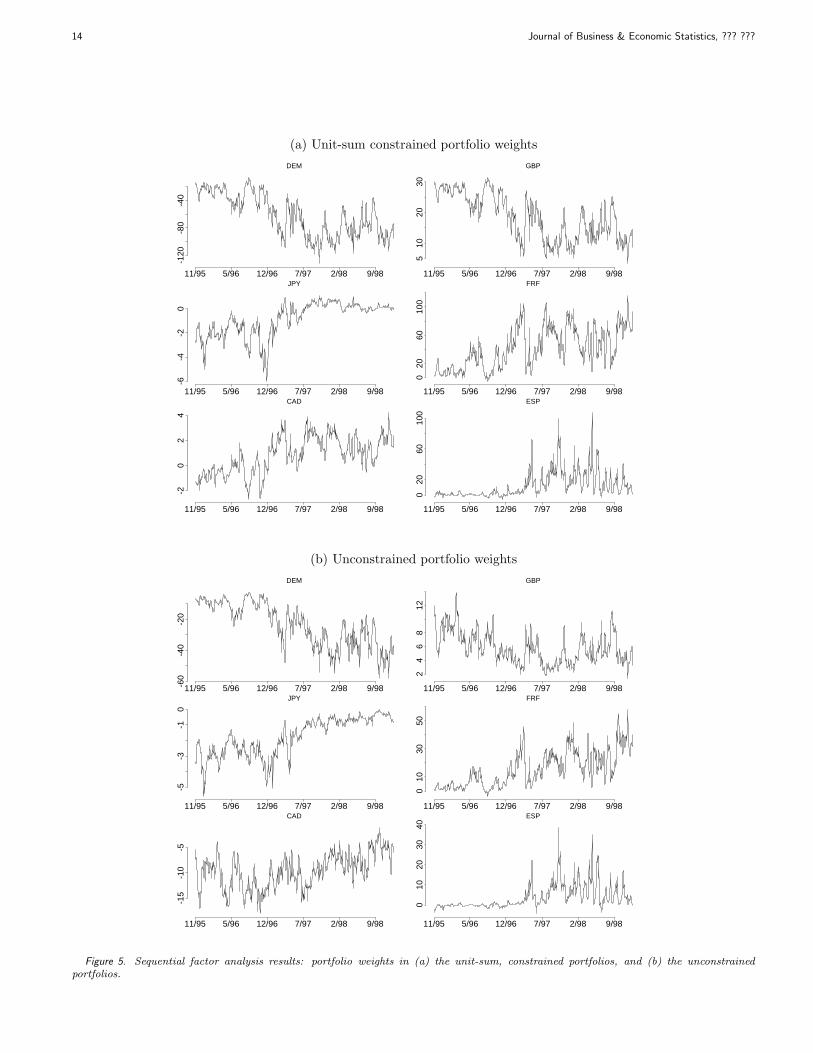
now detailed. Figure 5 graphs trajectories of the opti-mal portfolio weights in both the unit-sum, constrainedportfolios (frames (a)) and the unconstrained portfolios(frames (b)). Figure 7 graphs trajectories of cumulativereturns from both the constrained and unconstrained port-folio studies, compared with those from the optimal dis-count model. As a benchmark of poor performance, thereturns from the equally weighted portfolio at = 1/6 foreach t are also graphed. The figure displays returns cumu-lated over moving 30- and 90-day periods, and also acrossthe entire period from t = 1001 to the end of the dataframe. In viewing the four frames in this figure, note thediffering scales of the returns axis, chosen for clarity ofpresentations.

In viewing these graphs it is important to bear in mindthat our study is focussed wholly on the impact on portfo-lios of changing patterns of volatility, and on comparisonsof different models of volatility. We are not modelling dy-namic structure in the means of returns, so the constantestimate of expected returns used across the time periodis simply the posterior mean g of θ based on the MCMCanalysis up to t = 1000. In particular, the first elementof g is negative, implying a negative expected return onDEM around the end of 1995. This is reflected in the port-folios across the time period up to the end of 1998 throughnegative portfolio weights on DEM, i.e., the portfolios areshort on the German mark. More discussion on this ap-pears below.

Among the notable features of the trajectories of con-strained portfolio weights in Figure 5(a) are the fact thatboth JPY and CAD have generally very low weights acrossthe period. The elements of g indicate a mean for CADvery close to zero, as is expected on economic grounds.Also, note that the weights on JPY move towards zeroin the later periods of very high idiosyncratic volatility,reflecting increased risk aversion with respect to that cur-rency. In connection with the short positions on DEMdriven by the negative element of θ, note that, as it hap-

pens, both constrained and unconstrained portfolios adoptcorresponding long positions on FRF, and the portfolioweights on DEM and FRF essentially offset each other.

Comparison of Figures 5(a) and 5(b) indicate very sim-ilar patterns in the trajectories of portfolio weights. Whatis more interesting is that the unconstrained portfoliosadopt overall short positions across the period, as evi-denced by the trajectory of a′

tg in Figure 6. This isstrongly influenced by the negative mean, and resultingshort positions, for DEM, and reflects the response of theportfolio to the levels of volatility that, across the period,are generally high relative to the target mean return.

Comparison of these two factor model portfolios aresharpened in examination of the cumulative returns arisingunder each across this time period, in frames (a) and (b) ofFigure 7. The full line in Figure 7(a) represents the cumu-lative return over the entire period using the constrainedportfolio in the factor model; that in Figure 7(b) is thereturn using the unconstrained portfolio. The main pointis clear: the lack of a resource constraint – in this case,implying access to unlimited short positions – leads to theunconstrained portfolio outperforming the constrained bya factor of nearly 4 over this period of 827 days.

Also graphed in Figure 7(a) are the cumulative returnsresulting from the constrained portfolio used in the op-timal discount model (as a dotted line), and from thenaive, equal-weight portfolio (dashed line). It is evidentthat, when compared using the same constrained portfo-lio strategy, the use of sequential updating in the factormodel clearly dominates the optimal discount approach.The corresponding trajectories in Figure 7(b) confirm thisconclusion in the case of unconstrained portfolios.

Finally, frames (c) and (d) of Figure 7 display trajecto-ries of cumulative returns over shorter investment horizons– 30 days and 90 days, respectively. In each, the full linerepresents the factor model with unconstrained portfolios,the dotted line represents the optimal discount model withunconstrained portfolios, and the dashed line represents

$-2

.0-1

.5-1

.0-0

.50.

0

11/95 5/96 12/96 7/97 2/98 9/98

Figure 6. Sequential factor analysis results: Total implied investments in the unconstrained portfolios.


cum

ulat

ive

retu

rns

%-1

00

1020

3040

11/95 5/96 12/96 7/97 2/98 9/98

FDE

(a)

cum

ulat

ive

retu

rns

%-2

020

6010

0

11/95 5/96 12/96 7/97 2/98 9/98

(b)

(30)

cum

ulat

ive

retu

rns

%-1

00

1020

11/95 5/96 12/96 7/97 2/98 9/98

(c)

(90)

cum

ulat

ive

retu

rns

%-1

00

1020

3011/95 5/96 12/96 7/97 2/98 9/98

(d)

Figure 7. Sequential factor analysis results: Cumulative returns from factor (“F”) and discount (“D”) model-based portfolios, togetherwith those from a basic equally weighted (“E”) portfolio. (a) constrained portfolio, overall returns; (b) unconstrained portfolio, overallreturns; (c) 30 day returns from unconstrained portfolios; (d) 90 day returns from unconstrained portfolios.

the naive, equal-weight portfolio. Here the similarities inportfolio performance between the discount methods anddynamic factor models are really very clear. The major dif-ferences arise in the periods of radically increased volatil-ity, where the factor model is able to capitalise markedly interms of short-term gains relative to the discount method.This shorter term responsiveness in the factor models leadsto marked swings in portfolio structure that the uncon-strained allocations significantly capitalise upon, and thishas a persistent effect on overall cumulative returns there-after.

6. ADDITIONAL DISCUSSION AND CONCLUDING

COMMENTS

Our investigations indicate the feasibility of formalBayesian analysis of structured dynamic factor models.The analysis is accessible computationally with nowa-days moderate computational resources, and our empiri-cal studies suggest that the analysis will be manageablewith 20-30 dimensional time series and several factors.We are currently investigating more extensive applicationsin short-term forecasting and on-line portfolio allocationswith higher dimensional models for longer-term exchangerate futures. The example here is suggestive of poten-tial benefits, and supportive of the view that exploiting

systematic volatility patterns via factor structuring mayyield substantial improvements in short-term forecastingand decision making in dynamic portfolio allocation, es-pecially in the unconstrained optimisation. The discountmethod does reasonably well at times, though is clearlyeventually dominated in terms of cumulative return trajec-tories by the factor model. To partly offset this, however,we note that the shorter term focuses in Figure 7(c) and(d) indicate that the overall dominance of the factor modelapproach is partly based on its ability to adapt quickly to asmall number of major changes in volatility patterns. Forthis reason, financial analysts might prefer the more eas-ily implemented discount methods coupled with informedprospective interventions.

The dynamic factor models illustrated are amenableto direct implementation using our customised MCMCmethods with the minimal/reference prior specificationswe have used here. Our use of the variance discountingmethod on a reserved initial section of the data to pro-vide input to informative priors is important in identify-ing “ball-park” scales for the U matrix of the VAR(1) SVmodel. Though not pursued here, other aspects of suchpreliminary analyses may be used to determine informa-tive priors for other elements of the factor model. Theestablished discounting methods are, relative to dynamicfactor models, trivial to implement in the current context,a fact that is important in using discount methods to spec-


ify partial prior structure in the dynamic models. Ourempirical findings indicate that, not surprisingly with thiskind of data, moderately adaptive discount methods farewell in time of slow change in volatility levels and patterns,but are relatively uncompetitive in cases of more markedstructural change. This is to be expected. Looking ahead,models and approaches that attempt to simplify the pro-cess of factor modelling, perhaps somehow integrating ele-ments and concepts of variance matrix discounting into aspecified factor structure, may be attractive from a com-putational/implementation viewpoint. We are currentlyinvestigating such a synthesis of approaches.

In the factor model context per se, one of the importantfeatures in our model is the use of correlated innovations inthe multivariate AR model for the factor volatilities. Theapplied relevance of this is quite apparent from the ex-ploratory analyses using discount models, and confirmedin the factor model analysis through the posterior distri-butions for both factor volatilities and the correlation pa-rameters. Some important practical issues relate to thequestions of the ordering of individual time series underthe specific structure we adopt for factor loadings, and tothe choice and assessment of the number of factors. Onthe first issue, it needs to be restressed that, from theviewpoint of forecasting and portfolio allocations, the or-dering is irrelevant. The ordering is, of course, relevantin connection with model fitting and assessment, the in-terpretation of factors if such is desired, and the choiceof the number of factors. It is often desirable to use aspecific ordering to define and interpret the factors. Insuch cases, the ordering becomes a modelling decision tobe made on substantive grounds, rather than an empiricalmatter to be addressed on the basis of model fit. This isof particular relevance in connection with the potential forfactor models to improve sequential decisions by allowinginformed interventions on specific factors. For example,having identified the “Japan” factor in our financial timeseries model, we now have opportunities for selective in-terventions. Anticipating a specific change in Japanese fi-nancial policy, for example, we may intervene to “current”prior distributions for parameters related only to that fac-tor in the model. Such potential for selective interventionswas, in fact, one of our key initial motivations for exploringfactor models, and provides, we believe, a major incentivefor practitioners to take interest.

In connection with the ordering and the number of fac-tors, we report some initial results and experiences in staticfactor models – with constant volatilities – in Lopes andWest (1998). That work extends MCMC analysis of fac-tor models to include inference on the number of factors.Potential exists to develop such approaches to dynamicfactor models, although that is currently unexplored. Ofmore direct interest here, perhaps, are empirical findingsin a range of practical studies with the exchange rate se-ries. First, running MCMC analyses in models with toomany factors generally leads to problems in convergenceof the simulations. For example, in a model with threefactors when the data are really consistent with just two,

the simulated values of the third factor will naturally beclose to zero, although the MCMC will behave poorly andshow evidence of non-convergence. We have experiencedthis in studies of the exchange rates prior to 1992 in anextended data set going to back to 1986. Before the with-drawal of the UK from the ERM in fall 1992, the GBPseries generally tended to follow the European pattern,dominated by the DEM factor. The series prior to thatpoint are much better explained with a two factor model– one EU factor and one Japan factor – than with three,and the above problem of non-convergence of the MCMCarose. After fall 1992, a three factor model is much moreappropriate, with the third GBP factor explaining mean-ingful levels variation in the FRF and ESP series as wellas those of the GBP series. Methodologically, we concludethat poor convergence characteristics can point to a modelmis-specified with too many factors. The reverse of this,a model with too few factors, is rather more readily iden-tified through patterns of co-movements in the estimatedtrajectories of the idiosyncratic variances, consistent withone or more additional factors. Again, we have experi-enced this in analysing the post-1992 series with a twofactor model. This kind of exploratory analysis is criticaland necessary to a full understanding of the use of thesemodels, and will remain so even when more formal meth-ods of learning the number of factors are available. Finally,these empirical studies point to a challenging and poten-tially most important issue – that the number of factorsitself is truly dynamic, with different numbers of factorsbeing relevant at different times.

Model extensions that are currently under investigationrelax the assumptions of constancy of the factor loadings,and possible non-normal conditional distributions for fac-tors. In this connection, we note very closely related de-velopments by Pitt and Shephard (1999b), who exploresimilar factor models and related computational schemesfor model fitting and sequential analysis (as mentionedearlier, the current work was developed independently of,and in parallel to, the work of Pitt and Shephard). Someof our recent work has extented the current frameworkto bring in dynamic regressions for the mean θt in linewith discount models in current implementations in majorbanks (Putnam and Quintana 1994; Quintana and Put-nam 1996). Obviously, serious practical implementationof factor models demand such extensions. Particularlyfor forecasting and portfolio allocation with longer termhorizons, such as 30-day exchange rate futures, we needextended models that incorporate dynamic regressions onrelative interest rates and other possibly econometric in-dicators. Additional studies and empirical assessments ofthe methods on time series with larger numbers of uni-variate components and larger numbers of factors are alsounder investigation. Our experience to date leads us to be-lieve that such investigations will be fruitful and supportthe preliminary conclusions reached in this report aboutthe potential utility of factor models.


APPENDIX A: VARIANCE MATRIX DISCOUNTING

A brief summary of the basic method of variance ma-trix discounting are given here. As made clear by Uh-lig (1994) these methods have formal theoretical bases inmatrix-variate “random walks,” though they had been inuse by Quintana and coauthors (see references in the In-troduction) and others for several years prior to that work.As summarised in West and Harrison (1997, chapter 16),the models involve sequential updating of posterior distri-butions for the sequences of variance matrices Σt, with thefollowing ingredients.

At a specific time t, the current posterior for Σt is aninverse Wishart form. Using the notation of West and Har-rison (1997, chapter 16), the time t posterior is of the formp(Σt|Dt) = W−1

nt(Σt|St) where Dt = {D0,y1, . . . ,yt} =

{Dt−1,yt} is the sequentially updated information set attime t. Here nt is the degrees of freedom and St a posteriorestimate of Σt, the posterior harmonic mean. The nota-tion W−1

r (·|S) indicates the inverse Wishart distributionwith r degrees of freedom and scale matrix S (see West andHarrison, as referenced). In the special case of zero-meanobservations yt, the sequence of estimates St is triviallyupdated sequentially in time by the forward exponentialmoving average formula

St = (1 − at)St−1 + atyty′

t (8)

where the weight at is given by at = 1/(1 + δnt−1) basedon a discount factor δ. This discount factor lies in (0, 1),is typically between 0.9 and 1 and will be very close tounity for data at high sampling rates. Having analysed afixed stretch of data t = 1, . . . , n, the sequence of estimatesSt is revised by the related backward smoothing formulato incorporate the data at times t + 1, . . . , n in inferenceon Σt. Denoting the revised estimate of Σt by St,n, theformula is given in terms of inverse variance matrices bythe backward recursion

S−1t,n = (1 − δ)S−1

t + δS−1t+1,n (9)

for each t = n − 1, n− 2, . . . , 1, and starting with Sn,n =Sn. See West and Harrison (1997, pp608-609) for furtherdetails, and the references by Quintana and coauthors fordevelopment and applications in finance.

Extensions to models in which the time series has anunknown level θ or, more generally, a dynamic regressioncomponent θt, are straightforward. Then the observationyt is replaced by an appropriately scaled one-step aheadforecast error in the updating equation for St. The detailsare standard and a side issue here, though the modifi-cation is critical in developing portfolio allocations. Theresulting filtering and smoothing equations from Bayesiandiscounting analyses are modified following West and Har-rison (1997, pp608-609).

APPENDIX B: MCMC DEVELOPMENT

In each of the following subsections we detail the con-ditional posteriors for various parameters and latent vari-ables in turn. At each step it is implicit that we are con-ditioning on fixed values (previously simulated values) ofall other variables. As noted in the text, further technicaldetails are available on request from the authors. Our cur-rent implementation is in Fortran77 using standard ran-dom variate generation methods from RANDLIB.

Sampling the conditional meanThe basic model for yt and the uniform prior for θ imme-

diately imply a multivariate normal conditional posteriorfor θ given the values of Σt. This is easily sampled.

Sampling the latent factorsThe full conditional distribution of ft is given by

N(ft|At(yt − θ),Ht −AtQtA′

t)

where Qt = XHtX′ + Ψt and At = HtX

′Q−1t . The ft

are conditionally independent and so sample values aredrawn independently from this set of normal distributionsfor t = 1, 2 . . . , n.

Sampling the factor loadingsFrom the model, the conditional likelihood function for

the factor loading matrix X is∏n

t=1N(yt − θ|Xft,Ψt).This is a standard form, log-quadratic in the uncertainelements of X, and so combines with a normal or uniformreference prior to imply a multivariate normal conditionalposterior, which is easily sampled.

Sampling the mean of the factor SV VAR(1) modelUnder a normal prior N(µ|m0,M0), the conditional

posterior is normal N(µ|m,M) with

M−1 = M−10 + W−1 + (n− 1)(I− Φ)U−1(I − Φ)

and

Mm = M−10 m0 +W−1λ1 + (I−Φ)U−1

n∑

t=2

(λt −Φλt−1).

The case of a uniform reference prior is recovered by set-ting M−1

0 = 0.

Sampling the VAR coefficients in the factor SV modelThe structure of the conditional posterior for Φ, and

the resulting Metropolis-Hastings strategy for simulation,is precisely as developed for component VAR models ina quite different context in West and Aguilar (1998) andAguilar and West (1997). Writing γt = λt − µ, note thatthe full conditional posterior density for Φ is proportionalto

p(Φ)N(γ1|0,W)n

∏

t=2

N(γt|Φγt−1,U)

where W = ΦWΦ+U is easily evaluated as a function ofΦ and U. Write φ = (φ1, . . . , φk)′ for the diagonal of Φ,


and E = diag(γt−1). Then the conditional posterior maybe written as proportional to

p(Φ)c(Φ)N(φ|b,B)

where

B−1 =

n∑

t=2

E′U−1E and Bb =

n∑

t=2

E′U−1γt

and

c(Φ) = |W|−I/2exp(−trace(W−1γ1γ′

1)/2).

Under independent normal or uniform priors for the φj ,the full conditional posterior distribution for Φ is the mul-tivariate normal N(φ|b,B) truncated to the (0, 1) regionsin each dimension, and then multiplied by the factor c(Φ).This may be sampled by several methods. We use aMetropolis Hastings algorithm that takes the truncatedmultivariate normal component as proposal distribution.That is, given a “current” value of φ, with correspond-ing matrices Φ and W, we sample a “candidate” vectorφ∗ from this truncated normal, compute the correspond-ing diagonal matrix Φ∗ and variance matrix W∗ such thatW∗ = Φ∗W∗Φ∗ + U, then accept this new φ vector withprobability

min{1, c(Φ∗)/c(Φ)}.

Sampling the U matrix in the factor SV modelAgain, the structure of the conditional posterior for the

innovations variance matrix U of the VAR(1) volatilitymodel is closely related to developments in a quite differ-ent context in West and Aguilar (1998) and Aguilar andWest (1997). Again using centred volatilities γt = λt − µ

for each t, we have a full conditional posterior for U pro-portional to

p(U)a(U)|U|−(n−1)/2exp(−trace(U−1G))

where

G =

n∑

t=2

(γt −Φγt−1)(γt −Φγt−1)′

and

a(U) = |W|−1/2exp(−trace(W−1γ1γ′

1)/2)

with W = ΦWΦ + U. Under a specified inverse WishartpriorW−1

r0(U|R0), this posterior density is proportional to

a(U)W−1r (U|R)

where r = r0 + n− 1 and rR = r0R0 + (n− 1)G. We usethis inverse Wishart distribution as a proposal distributionin the Metropolis-Hastings algorithm. That is, given a“current” value of U and corresponding W, we sample a“candidate” value U∗ from W−1

r (U|R), and accept it withprobability

min{1, a(U∗)/a(U)}where W∗ = ΦW∗Φ + U∗.

Sampling the factor volatility processesGiven currently imputed values for the full factor pro-

cess ft over time t, we follow Kim, Shephard and Chib(1998) in transforming each of the univariate time seriesof factor elements into a non-Gaussian linear model form.Specifically, for each factor i and time t define zti = log(f2

ti)and note that

zti = λti + νti

where the νti terms are independent and distributed aslog−χ2

1. In vector form for all k factor series, we then have

zt = λt + νt

where νt = (νt1, . . . , νtk)′. Based on the current values ofthe zt, for each t, this provides the set observation equa-tions for the dynamic linear model with state equations

λt = µ + Φ(λt−1 − µ) + ωt

for each t. This is a direct multivariate extension of theunivariate approach in Kim, Shephard and Chib (1998),whose ensuing analysis uses the now established approxi-mation to the distribution of the error terms νit as a speci-fied finite mixture of normals (Shephard 1994b). The mul-tivariate extension is immediate:

• Introduce a set of indicator variables lti such that ltiidentifies the normal mixture component for νti.

• Conditional on these indicators, we have a multivari-ate dynamic linear model for the sequence of log-volatility vectors. The forward-filtering, backward-sampling algorithm for state space models (Carterand Kohn 1994; Fruhwirth-Schnatter 1994; West andHarrison 1997, chapter 15) now applies to directlysimulate the full set of vectors {λt, t = 1, . . . , n}from the implied conditional posterior. (Note that,in more elaborate models for the volatility processes,the alternative sampling method using the simula-tion smoother of de Jong and Shephard (1995) mayhave computational advantages not realised in this,the simplest VAR model.)

• Given these sampled values of the λt, the completeconditional multinomial posterior probabilities overvalues of the indicators lit are easily computed, theindicators being conditionally independent and soeasily sampled.

Sampling idiosyncratic volatilitiesConditional on currently imputed values of θ,X and the

ft, we have imputed values of each of the error vectorsεt = (εt1, . . . , εtq)

′ in equation (2). This defines a set ofq independent and standard univariate SV models, as fol-lows: with vtj = log(ε2tj) for each j, t,

vtj = ηtj + τtj


where the τtj terms are independent and distributed aslog−χ2

1, and ηtj = log(ψtj) follow the AR(1) models ofsection 2.4, namely

ηtj = αj + ρj(ηt−1,j − αj) + ξtj

with independent innovations ξtj ∼ N(ξtj |0, sj). The stan-dard sampling schemes of Kim, Shephard and Chib (1998),and with minor modifications from West and Aguilar(1997), now apply to each of these j = 1, . . . , q univariateSV models. This produces imputed values for ηtj , hencethe volatilities ψtj , for each j = 1, . . . , q and for all t.

Sampling the means in the idiosyncratic SV modelsConditional on currently imputed values of each of the

ηtj , the univariate SV models imply standard likelihoodfunctions for each of the means αj , independently acrossseries j. Under independent normal priors, or standard ref-erence uniform priors, these lead to independent normalposteriors that are trivially sampled.

Sampling the ρtj in the idiosyncratic SV modelsConditional on currently imputed values of each of the

ηtj , the univariate SV models imply likelihood functionsfor each of the ρj , independently across series j. Theseare precise univariate analogues of the likelihood functionsfor the VAR parameter matrix Φ discussed above, andthe simulation strategy there is applied, in its univariateanalogue, to each of these q models to impute new valuesfor each of the ρj .

Sampling the sj in the idiosyncratic SV modelsConditional on currently imputed values of each of the

ηtj , the univariate SV models imply likelihood functionsfor each of the sj , independently across series j. These areagain precise univariate analogues of the likelihood func-tions for the VAR parameter matrix U discussed above.The structure simplifies in that the inverse Wisharts in themultivariate case are replaced by inverse gamma distribu-tions for the sj , but otherwise the general strategy is thesame. This is applied, in each of the q models in parallel,to impute new values for each of the sj .

REFERENCES

Aguilar, O., and West M. (1998), “Analysis of Hospital QualityMonitors using Hierarchical Time Series Models,” in Case StudiesBayesian Statistics in Science and Technology: Case Studies 4,(eds: C. Gatsonis et al), Springer-Verlag, New York, 287-302.

Ameen, J.R., and Harrison, P.J. (1985), “Normal Discount BayesianModels,” in Bayesian Statistics 2, (eds: J.M. Bernardo, M.H. DeGroot, D.V. Lindley and A.F.M. Smith), North Holland, Amster-dam, and Valencia University Press, 271-298.

Carter, C., and Kohn, R. (1994), “On Gibbs Sampling for StateSpace Models,” Biometrika, 81, 541–553.

Demos, A., and Sentana, E. (1998), “An EM Algorithm for Condi-tionally Heteroskedastic Factor Models,” Journal of Business andEconomic Statistics, 16, 357-361.

Fruhwirth-Schnatter, S. (1994), “Data Augmentation and DynamicLinear Models,” Journal of Time Series Analysis, 15, 183–202.

de Jong, P., and Shephard, N. (1995), “The Simulation Smoother forTime Series Models,” Biometrika, 82, 339-50.

Geweke, J.F., and Singleton, K.J. (1980), “Interpreting the Likeli-hood Ratio Statistic in Factor Models when Sample Size is Small,”

Journal of the American Statistical Association, 75, 133-137.

Geweke, J.F., and Zhou, G. (1996), “Measuring the Pricing Error ofthe Arbitrage Pricing Theory,” The Review of Financial Studies,9, 557-587.

Harrison, P.J., and West, M. (1987), “Practical Bayesian Forecast-ing,” The Statistician, 36, 115-125.

Harvey, A.C., Ruiz, E. and Shephard, N. (1994), “MultivariateStochastic Variance Models,” Review of Economic Studies, 61,247-264.

Jacquier, E., Polson, N.G., and Rossi, P. (1994), “Bayesian Analy-sis of Stochastic Volatility Models (with Discussion),” Journal ofBusiness and Economic Statistics, 12, 371-388.

Jacquier, E., Polson, N.G. and Rossi, P. (1995), “Models and Priorsfor Multivariate Stochastic Volatility,” Discussion Paper, Gradu-ate School of Business, University of Chicago.

Kim, S., Shephard, N. and Chib, S. (1998), “Stochastic Volatility:Likelihood Inference and Comparison with ARCH Models,” Re-view of Economic Studies, 65, 361-393.

Liu, J., and West, M. (2000), “Combined Parameter and State Esti-mation in Simulation-based Filtering,” in Sequential Monte CarloMethods in Practice, (eds: A. Doucet, J. F. G. De Freitas, andN.J. Gordon), New York: Springer-Verlag (forthcoming).

Lopes, H.F., and West, M. (1998), “Model Uncertainty in FactorAnalysis,” Discussion Paper #98-38, Institute of Statistics andDecision Sciences, Duke University.

Pitt, M.K., and Shephard, N. (1999a), “Filtering via Simulation:Auxiliary Particle Filters,” Journal of the American StatisticalAssociation, 94, 590-599.

Pitt, M.K., and Shephard, N. (1999b), “Time Varying Covariances:A Factor Stochastic Volatility Approach.,” (with Discussion), inBayesian Statistics 6 (J. M. Bernardo, J. O. Berger, A. P. Dawidand A. F. M. Smith, eds.). Oxford: University Press, 547-570.

Polson, N.G., and Tew, B.V. (1997), “Bayesian Portfolio Selection:An Empirical Analysis of the SP500 Index 1970-1996,” DiscussionPaper, Graduate School of Business, University of Chicago.

Press, S.J. (1985), Applied Multivariate Analysis: Using Bayesianand Frequentist Methods of Inference, California: Krieger.

Press, S.J., and Shigemasu, K. (1989), “Bayesian Inference in Fac-tor Analysis,” in Contributions to Probability and Statistics: Es-says in Honor of Ingram Olkin, (eds: L.J. Gleser, M.D. Perlman,S.J. Press and A.R. Sampson,), New York: Springer Verlag, 271-287.

Putnam, B.H., and Quintana, J.M. (1994), “New Bayesian Statis-tical Approaches to Estimating and Evaluating Models of Ex-change Rates Determination,” In Proceedings of the ASA Sectionon Bayesian Statistical Science, 1994 Joint Statistical Meetings,American Statistical Association.

Putnam, B.H., and Quintana, J.M. (1995), “The Evolution ofBayesian Forecasting Models,” in Asset Allocation: ApplyingQuantitative Discipline to Asset Allocation, (ed: B.H. Putnam),London: Global Investor, Euromoney Publications, 139-146.

Quintana, J.M., and West, M. (1987), “An Analysis of InternationalExchange Rates using Multivariate DLMs,” The Statistician, 36,275-281.

Quintana, J.M., and West, M. (1988), “Time Series Analysis of Com-positional Data,” in Bayesian Statistics 3, (eds: J.M. Bernardo,M.H. De Groot, D.V. Lindley and A.F.M. Smith), Oxford Univer-sity Press, 747-756.

Quintana, J.M. (1992), “Optimal Portfolios of Forward Cur-rency Contracts,” in Bayesian Statistics 4, (eds: J.O. Berger,J.M. Bernardo, A.P. Dawid and A.F.M. Smith), Oxford UniversityPress.

Quintana, J.M., Chopra, V.K., and Putnam, B.H. (1995), “GlobalAsset Allocation: Stretching Returns by Shrinking Forecasts,” inProceedings of the ASA Section on Bayesian Statistical Science,1995, Joint Statistical Meetings, American Statistical Association.

Quintana, J.M., and Putnam, B.H. (1996), “Debating Currency Mar-kets Efficiency using Multiple-Factor Models,” in Proceedings ofthe ASA Section on Bayesian Statistical Science, 1996 Joint Sta-tistical Meetings, American Statistical Association.

Shephard, N. (1994a), “Local Scale Models: State Space Alternativesto Integrated GARCH Processes,” Journal of Econometrics, 6,

21

333-364.

Shephard, N. (1994b), “Partial Non-Gaussian State Space,”Biometrika, 81, 115-132.

Shephard, N. (1996), “Statistical Aspects of ARCH and Stochas-tic Volatility,” in Time Series Models in Econometrics, Financeand Other Fields, (eds: D.R. Cox, O.E. Barndorff-Nielson andD.V. Hinkley), London: Chapman & Hall, 1-67.

Shephard, N., and Pitt, M.K. (1997), “Likelihood Analysis of Non-Gaussian Measurement Time Series,” Biometrika, 84, 653-67.

Uhlig, H. (1994), “On Singular Wishart and Singular MultivariateBeta Distributions,” Annals of Statistics, 22, 395-405.

Uhlig, H. (1997), “Bayesian Vector-Autoregressions with StochasticVolatility,” Econometrica, 65, 59-73.

West, M. (1993), “Mixture models, Monte Carlo, Bayesian Updatingand Dynamic Models,” Computing Science and Statistics, 24, 325-333.

West, M., and Aguilar, O. (1997), “Studies of Quality Monitor TimeSeries: The V.A. Hospital System,” report for the VA ManagementScience Group, Bedford, MA., Institute of Statistics and DecisionSciences, Discussion Paper #96-02.

West, M., and Harrison, P.J. (1997), Bayesian Forecasting and Dy-namic Models, (2nd Edn.), New York: Springer Verlag.

bayesian dynamic factor models and portfolio...

Documents