Portfolio Allocation for Bayesian Optimization

Matthew Hoffman, Eric Brochu, Nando de FreitasDepartment of Computer Science

University of British ColumbiaVancouver, Canada

{hoffmanm,ebrochu,nando}@cs.ubc.ca

Abstract

Bayesian optimization with Gaussian pro-cesses has become an increasingly populartool in the machine learning community. Itis efficient and can be used when very littleis known about the objective function, mak-ing it popular in expensive black-box opti-mization scenarios. It uses Bayesian methodsto sample the objective efficiently using anacquisition function which incorporates theposterior estimate of the objective. However,there are several different parameterized ac-quisition functions in the literature, and it isoften unclear which one to use. Instead of us-ing a single acquisition function, we adopt aportfolio of acquisition functions governed byan online multi-armed bandit strategy. Wepropose several portfolio strategies, the bestof which we call GP-Hedge, and show thatthis method outperforms the best individ-ual acquisition function. We also provide atheoretical bound on the algorithm’s perfor-mance.

1 INTRODUCTION

Bayesian optimization is a powerful strategy for find-ing the extrema of objective functions that are expen-sive to evaluate. It is applicable in situations whereone does not have a closed-form expression for theobjective function, but where one can obtain noisyevaluations of this function at sampled values. It isparticularly useful when these evaluations are costly,when one does not have access to derivatives, or whenthe problem at hand is non-convex. Bayesian opti-mization has two key ingredients. First, it uses theentire sample history to compute a posterior distribu-tion over the unknown objective function. Second, ituses an acquisition function to automatically trade offbetween exploration and exploitation when selecting

the points at which to sample next. As such, Bayesianoptimization techniques are some of the most efficientapproaches in terms of the number of function evalu-ations required [30, 23, 25, 3, 5]. The term Bayesianoptimization was coined in the seventies [30], but aversion of the method has been known as EfficientGlobal Optimization (EGO) in the experimental de-sign literature since the nineties [37]. In recent years,the machine learning community has increasingly usedBayesian optimization to optimize expensive objectivefunctions. Examples can be found in robot gait design[26], online path planning [28, 29], intelligent user in-terfaces for animation [6, 4], algorithm configuration[20], efficient MCMC [34], sensor placement [38, 33],and reinforcement learning [5]. Consistency of themethod was shown in [27] for 1D processes and in[39] for general Gaussian processes with an acquisitionfunction known as expected improvement. Rates ofconvergence for an acquisition function, known as up-per confidence bound, were provided last year in [38].A more recent report [9] discusses more general con-vergence rates. We refer readers interested in a morein depth review of Bayesian optimization to [5].

Our main argument is that the choice of acquisitionfunction is not trivial. Several different acquisitionfunctions have been proposed in the literature, none ofwhich work well for all classes of functions. Buildingon recent developments in the field of online learningand multi-armed bandits [10], this paper proposes asolution to this problem. The solution is based on ahierarchical hedging approach for managing an adap-tive portfolio of acquisition functions.

The paper will show that the proposed strategy ofcombining acquisition functions results in large im-provements over the single acquisitions strategies pro-posed in statistics and optimization (expected im-provement) and more recently in machine learning (up-per confidence bounds). This will be shown with syn-thetic experiments (so that we can assess the effect ofdimensionality), a suite of optimization problems bor-

rowed from the global optimization literature (some ofwhich are repeatedly cited as being very hard) and ahard, nonlinear, 9D continuous Markov decision pro-cess with a reward that has many modes and relativelylarge plateaus in between. The nature of the rewardfunction in the control problem will cause gradientmethods to do much worse than the Bayesian opti-mization strategies. Finally, the paper will also presenta theoretical analysis of the proposed techniques.

We review Bayesian optimization and popular acqui-sition functions in Section 2. In Section 3, we proposethe use of various hedging strategies for Bayesian opti-mization [2, 11]. In Section 4, we present experimentalresults using standard test functions from the litera-ture of global optimization. The experiments showthat the proposed hedging approaches outperform anyof the individual acquisition functions. We also pro-vide detailed comparisons among the hedging strate-gies. Finally, in Section 5 we present a bound on thecumulative regret which helps provide some intuitionas to algorithm’s performance.

2 BAYESIAN OPTIMIZATION

We are concerned with the task of optimization on ad-dimensional space: maxx∈A⊆Rd f(x).

We define xt as the tth sample and yt = f(xt)+εt, with

εtiid∼ N (0, σ2), as a noisy observation of the objective

function at xt. Other observation models are possible[5, 12, 14, 36], but we will focus on real, Gaussianobservations for ease of presentation.

The Bayesian optimization procedure is shown in Al-gorithm 1. As mentioned earlier, it has two com-ponents: the posterior distribution over the objec-tive and the acquisition function. Let us focus onthe posterior distribution first and come back to theacquisition function in Section 2.2. As we accumu-late observations1 D1:t = {x1:t, y1:t}, a prior distri-bution P (f) is combined with the likelihood func-tion P (D1:t|f) to produce the posterior distribution:P (f |D1:t) ∝ P (D1:t|f)P (f). The posterior capturesthe updated beliefs about the unknown objective func-tion. One may also interpret this step of Bayesian op-timization as estimating the objective function with asurrogate function (also called a response surface). Wewill place a Gaussian process (GP) prior on f . Othernonparametric priors over functions, such as randomforests, have been considered [5], but the GP strategyis the most popular alternative.

1Here we use subscripts to denote sequences of data, i.e.y1:t = {y1, . . . , yt}.

Algorithm 1 Bayesian Optimization

1: for t = 1, 2, . . . do2: Find xt by optimizing the acquisition function over

the GP: xt = argmaxx u(x|D1:t−1).3: Sample the objective function: yt = f(xt) + εt.4: Augment the data D1:t = {D1:t−1, (xt, yt)}.

5: end for

2.1 GAUSSIAN PROCESSES

The objective function is distributed according to a GPprior: f(x) ∼ GP(m(x), k(xi,xj)). For convenience,and without loss of generality, we assume that the priormean is the zero function (but see [29, 35, 4] for ex-amples of nonzero means). This leaves us the more in-teresting question of defining the covariance function.A very popular choice is the squared exponential ker-nel with a vector of automatic relevance determination(ARD) hyperparameters θ [35]:

k(xi,xj) = exp(− 1

2 (xi − xj)T diag(θ)−2(xi − xj)

),

where diag(θ) is a diagonal matrix with entries θ alongthe diagonal and zeros elsewhere. The choice of hy-perparameters will be discussed in the experimentalsection, but we note that it is not trivial in this do-main because of the paucity of data. For an in depthanalysis of this issue we refer the reader to e.g. [4, 33].

We can sample the GP at t points by choosing theindices {x1:t} and sampling the values of the functionat these indices to produce the data D1:t. The func-tion values are distributed according to a multivariateGaussian distributionN (0,K), with covariance entriesk(xi,xj). Assume that we already have the observa-tions, say from previous iterations, and that we wantto use Bayesian optimization to decide what point xt+1

should be considered next. Let us denote the value ofthe function at this arbitrary point as ft+1. Then, bythe properties of GPs, f1:t and ft+1 are jointly Gaus-sian: [

f1:tft+1

]∼ N

(0,

[K kkT k(xt+1,xt+1)

]),

where k = [k(xt+1,x1), k(xt+1,x2), . . . , k(xt+1,xt)].Using the Sherman-Morrison-Woodbury formula, see[35] for a comprehensive treatment, one can easily ar-rive at an expression for the predictive distribution:

P (yt+1|D1:t,xt+1) = N (µt(xt+1), σ2t (xt+1) + σ2),

where

µt(xt+1) = kT [K + σ2I]−1y1:t,

σ2t (xt+1) = k(xt+1,xt+1)− kT [K + σ2I]−1k.

In this sequential decision making setting, the numberof query points is relatively small and, consequently,the GP predictions are easy to compute.

Figure 1: Acquisition functions with different values of theexploration parameters ν and ξ. The GP posterior is shownat the top. The other images show the acquisition functionsfor that GP. From the top: Probability of improvement,expected improvement and upper confidence bound. Themaximum of each acquisition function, where the GP is tobe sampled next, is shown with a triangle marker. Note theincreased preference for exploration exhibited by GP-UCB.

2.2 ACQUISITION FUNCTIONS

The role of the acquisition function is to guide thesearch for the optimum. Typically, acquisition func-tions are defined such that high values correspondto potentially high values of the objective function,whether because the prediction is high, the uncer-tainty is great, or both. The acquisition function ismaximized to select the next point at which to evalu-ate the objective function. That is, we wish to sam-ple the objective function at argmaxx u(x|D). Thisauxiliary maximization problem, where the objectiveis known and easy to evaluate, can be easily carriedout with standard numerical techniques such as multi-start, sequential quadratic programming or DIRECT[22, 16, 32]. The acquisition function is sometimescalled the infill or simply the “utility” function. Inthe following sections, we will look at the three mostpopular choices. Figure 1 shows how these give rise todistinct sampling behaviour.

Probability of improvement (PI): The early workof Kushner [24] suggested maximizing the probabilityof improvement over the incumbent µ+ = maxt µ(xt).The drawback, intuitively, is that this formulation isbiased toward exploitation only. To remedy this, prac-titioners often add a trade-off parameter ξ ≥ 0, so that

PI(x) = P (f(x) ≥ µ+ + ξ) = Φ

(µ(x)− µ+ − ξ

σ(x)

),

where Φ(·) is the standard Normal cumulative distri-bution function (CDF). The exact choice of ξ is leftto the user. Kushner recommends using a (unspeci-fied) schedule for ξ, which should start high in orderto drive exploration and decrease towards zero as thealgorithm progresses. Lizotte, however, found that us-ing such a schedule did not offer improvement over aconstant value of ξ on a suite of test functions [25].

Expected improvement (EI): More recent workhas tended to take into account not only the probabil-ity of improvement, but the magnitude of the improve-ment a point can potentially yield. Mockus et al. [30]proposed maximizing the expected improvement withrespect to the best function value yet seen, given bythe incumbent x+ = argmaxxt

f(xt). For our Gaus-sian process posterior, one can easily evaluate this ex-pectation, see [21], yielding:

EI(x) =

{dΦ(d/σ(x)) + σ(x)φ(d/σ(x)) if σ(x) > 0

0 if σ(x) = 0

where d = µ(x)−µ+−ξ and where φ(·) and Φ(·) denotethe PDF and CDF of the standard Normal distributionrespectively. Here ξ is an optional trade-off parameteranalogous to the one defined above.

Upper confidence bound (UCB & GP-UCB):Cox and John [13] introduce an algorithm they call“Sequential Design for Optimization”, or SDO. Givena random function model, SDO selects points for eval-uation based on a confidence bound consisting of themean and weighted variance: µ(x) + κσ(x). As withthe other acquisition models, however, the parameterκ is left to the user. A principled approach to selectingthis parameter is proposed by Srinivas et al. [38]. Inthis work, the authors define the instantaneous regretof the selection algorithm as r(x) = f(x?)− f(x) andattempt to select a sequence of weights κt so as to min-imize the cumulative regret RT = r(x1) + · · ·+ r(xT ).Using the upper confidence bound selection criterionwith κt =

√νβt and the hyperparameter ν > 0 Srini-

vas et al. define

GP-UCB(x) = µ(x) +√νβtσ(x).

It can be shown that this method has cumulative re-gret bounded by O(

√TβT γT ) with high probability.

Here βT is a carefully selected learning rate and γT isa bound on the information gained by the algorithm atselected points after T steps. Both of these terms de-pend upon the particular form of kernel-function used,but for most kernels their product can be shown to besublinear in T . We refer the interested reader to theoriginal paper [38] for exact bounds.

The sublinear bound on cumulative regret implies thatthe method is no-regret, i.e. that limT→∞RT /T = 0.This in turn provides a bound on the convergence ratefor the optimization process, since the regret at themaximum f(x∗)−maxt f(xt) is upper bounded by the

average regret RT /T = f(x∗) − 1T

∑Tt=1f(xt). As we

will note later, however, this bound can be quite loosein practice.

Algorithm 2 GP-Hedge

1: Select parameter η ∈ R+.2: Set gi0 = 0 for i = 1, . . . , N .3: for t = 1, 2, . . . do4: Nominate points from each acquisition function:

xit = argmaxx ui(x|D1:t−1).

5: Select nominee xt = xjt with probability pt(j) =

exp(ηgjt−1)/∑k

`=1 exp(ηg`t−1).6: Sample the objective function yt = f(xt) + εt.7: Augment the data D1:t = {D1:t−1, (xt, yt)}.8: Receive rewards rit = µt(x

it) from the updated GP.

9: Update gains git = git−1 + rit.

10: end for

3 PORTFOLIO STRATEGIES

There is no choice of acquisition function that can beguaranteed to perform best on an arbitrary, unknownobjective. In fact, it may be the case that no sin-gle acquisition function will perform the best over anentire optimization — a mixed strategy in which theacquisition function samples from a pool (or portfo-lio) at each iteration might work better than any sin-gle acquisition. This can be treated as a hierarchicalmulti-armed bandit problem, in which each of the Narms is an acquisition function, each of which is it-self an infinite-armed bandit problem. In this sectionwe propose solving the selection problem using threestrategies from the literature, the application of whichwe believe to be novel.

Hedge is an algorithm which at each time step t se-lects an action i with probability pt(i) based on thecumulative rewards (gain) for that action (see Aueret al. [2]). After selecting an action the algorithm re-ceives reward rit for each action and updates the gainvector. In the Bayesian optimization setting, we candefine N bandits each corresponding to a single ac-quisition function. Choosing action i corresponds tosampling from the point nominated by function ui,

i.e. xit = argmaxx ui(x|D1:t−1) for i = 1, . . . , N . Fi-

nally, while in the conventional Bayesian optimizationsetting the objective function is sampled only once periteration, Hedge is a full information strategy and re-quires a reward for every action at every time step.We can achieve this by defining the reward at xi

t asthe expected value of the GP model at xi

t. That is,rit = µt(x

it). We refer to this method as GP-Hedge.

Provided that the objective function is smooth, thisreward definition is reasonable.

Auer et al. also propose the Exp3 algorithm, a vari-ant of Hedge that applies to the partial informationsetting. In this setting it is no longer assumed thatrewards are observed for all actions. Instead at eachiteration a reward is only associated with the partic-ular action selected. The algorithm uses Hedge as asubroutine where rewards observed by Hedge at eachiteration are rit/pt(i) for the action selected and zerofor all actions. Here pt(i) is the probability that Hedgewould have selected action i. The Exp3 algorithm,meanwhile, selects actions from a distribution that isa mixture between pt(i) and the uniform distribution.Intuitively this ensures that the algorithm does notmiss good actions because the initial rewards were low(i.e. it continues exploring).

Finally, another possible strategy is the NormalHedgealgorithm [11]. This method, however, is built to takeadvantage of situations where the number of banditarms (acquisition functions) is large, and may not bea good match to problems where N is relatively small.

The GP-Hedge procedure is shown in Algorithm 2.In practice any of these hedging strategies could beused, however in our experiments we find that Hedgetends to outperform the others. Note that it is neces-sary to optimize N acquisition functions at each timestep rather than 1. While this might seem expensive,this is unlikely to be a major problem in practice forsmall N , as (i) Bayesian optimization is typically em-ployed when sampling the objective is so expensive asto dominate other costs; (ii) it has been shown thatfast approximate optimization of u is usually sufficient[6, 25, 20]; and (iii) it is straightforward to run theoptimizations in parallel on a modern multicore pro-cessor.

We will also note that the setting of our problem issomewhere “in between” the full and partial informa-tion settings. Consider, for example, the situation thatall points sampled by our algorithm are “too distant”in the sense that the kernels evaluated at these pointsexert negligible influence on each other. In this case,we can see that only information obtained by the sam-pled point is available, and as a result GP-Hedge willbe over-confident in its predictions when using the full-

information strategy. However, this behaviour is notobserved in practical situations because of smoothnessproperties, as well as our particular selection of acqui-sition functions. In the case of adversarial acquisitionfunctions one might instead choose to use the Exp3variant.

4 EXPERIMENTS

To validate the use of GP-Hedge, we tested the opti-mization performance on a set of test functions withknown maxima f(x?). To see how effective eachmethod is at finding the global maximum, we use the“gap” metric [19], defined as

Gt =[f(x+)− f(x1)

]/[f(x?)− f(x1)

],

where again x+ is the incumbent or best function sam-ple found up to time t. The gap Gt will therefore bea number between 0 (indicating no improvement overthe initial sample) and 1 (if the incumbent is the max-imum). Note, while this performance metric is eval-uated on the true function values, this information isnot available to the optimization methods.

4.1 STANDARD TEST FUNCTIONS

We first tested performance using functions commonto the literature on Bayesian optimization: the Branin,Hartman 3, and Hartman 6 functions. All of these arecontinuous, bounded, and multimodal, with 2, 3, and6 dimensions respectively. We omit the formulae ofthe functions for space reasons, but they can be foundin [25]. These functions have been proposed by [15] asbenchmarks for comparing global search methods andare widely used for this purpose, see e.g. [22].

For each experiment, we optimized 25 times and com-puted the mean and variance of the gap metric overtime. In these experiments we used hyperparametersθ chosen offline so as to maximize the log marginallikelihood of a (sufficiently large) set of sample points;see [35]. We compared the standard acquisition func-tions using parameters suggested by previous authors,i.e. ξ = 0.01 for EI and PI, δ = 0.1 and ν = 0.2 forGP-UCB [25, 38]. For the GP-Hedge trials, we testedperformance under using both 3 acquisition functionsand 9 acquisition functions. For the 3-function variantwe use the standard acquisition functions with defaulthyperparameters. The 9-function variant uses thesesame three as well as 6 additional acquisition func-tions consisting of: both PI and EI with ξ = 0.1 andξ = 1.0, GP-UCB with ν = 0.1 and ν = 1.0. Whilewe omit trials of these additional acquisition functionsfor space reasons, these values are not expected to per-form as well as the defaults and our experiments con-firmed this hypothesis. However, we are curious to see

if adding known suboptimal acquisition functions willhelp or hinder GP-Hedge in practice.

Results for the gap measure Gt are shown in Figure 2.While the improvement GP-Hedge offers over the bestsingle acquisition function varies, there is almost nocombination of function and time step in which the 9-function GP-Hedge variant is not the best-performingmethod. The results suggest that the extra acquisi-tion functions assist GP-Hedge in exploring the spacein the early stages of the optimization process. Fig-ure 2 also displays, for a single example run, how thethe arm probabilities pt(i) used by GP-Hedge evolveover time. We have observed that the distributionbecomes more stable when the acquisition functionscome to a general consensus about the best region tosample. As the optimization progresses, exploitationbecomes more rewarding than exploration, resulting inmore probability being assigned to methods that tendto exploit. However, note that if the initial portfoliohad consisted only of these more exploitative acquisi-tion functions, the likelihood of becoming trapped atsuboptimal points would have been higher.

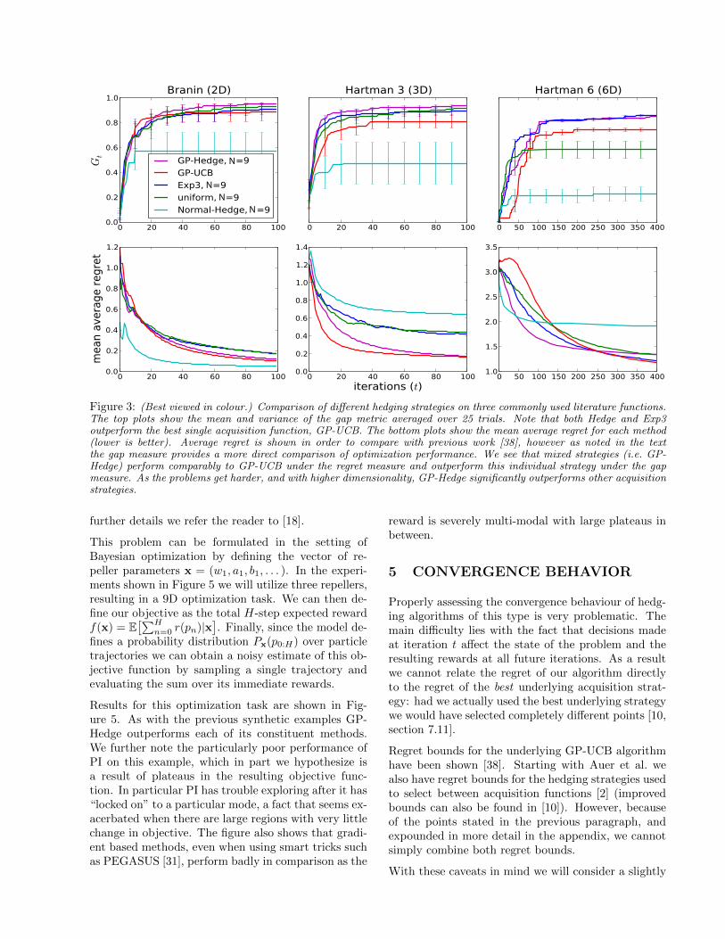
In Figure 3 we compare against the other Hedgingstrategies introduced in Section 3 under both the gapmeasure and mean average regret. We also intro-duce a baseline strategy which utilizes a portfolio uni-formly distributed over the same acquisition functions.The results show that mixing across multiple acquisi-tion functions provides significant performance ben-efits under the gap measure, and as the problems’difficulty/dimensionality increases we see that GP-Hedge outperforms other mixed strategies. The uni-form strategy performs well on the easier test func-tions, as the individual acquisition functions are rea-sonable. However, for the hardest problem (Hartman6) we see that the performance of the naive uniformstrategy degrades. NormalHedge performs particu-larly poorly on this problem. We observed that thisalgorithm very quickly collapses to an exclusively ex-ploitative portfolio which becomes very conservativein its departures from the incumbent. We again notethat this strategy is intended for large values of N ,which may explain this behaviour.

In the case of the regret measure we see that thehedging strategies perform comparable to GP-UCB,a method designed to optimize this measure. We fur-ther note that although the average regret can provequite useful in assessing the convergence behavior ofBayesian optimization methods, the bounds providedby this regret can be loose in practice. Further, inthe setting of Bayesian optimization we are typicallyconcerned not with the cumulative regret during opti-mization, but instead with the regret incurred by theincumbent after optimization is complete. Similar no-

NN

Figure 2: (Best viewed in colour.) Comparison of different acquisition approaches on three commonly used literaturefunctions. The top plots show the mean and variance of the gap metric averaged over 25 trials. We note that the top twoperforming algorithms use a portfolio strategy. With N = 3 acquisition functions, GP-Hedge beats the best-performingacquisition function in almost all cases. With N = 9, we add additional instances of the three acquisition functions, butwith different parameters. Despite the fact that these additional functions individually perform worse than the ones withdefault parameters, adding them to GP-Hedge improves performance in the long run. The bottom plots show an exampleevolution of GP-Hedge’s portfolio with N = 9 for each objective function. The height of each band corresponds to theprobability pt(i) at each iteration.

tions of “simple regret” have been studied in [1, 8].

Based on the performance in these experiments, weuse Hedge as the underlying algorithm for GP-Hedgein the remainder of the experiments.

4.2 SAMPLED TEST FUNCTIONS

As there is no generally-agreed-upon set of test func-tions for Bayesian optimization in higher dimensions,we seek to sample synthetic functions from a knownGP prior similar to [25]. For further details on howthese functions are sampled see Appendix A. As canbe seen in Figure 4, GP-Hedge with N = 9 is again thebest-performing method, which becomes even moreclear as the dimensionality increases. Interestingly,the worst-performing function changes as dimension-ality increases. In the 40D experiments, GP-UCB,which generally performed well in other experiments,does quite poorly. Examining the behaviour, it ap-pears that by trying to minimize regret instead ofmaximizing improvement, GP-UCB favours regions ofhigh variance. However, since a 40D space remainsextremely sparsely populated even with hundreds ofsamples, the vast majority of the space still has highvariance, and thus high acquisition value.

4.3 CONTROL OF A PARTICLESIMULATION

We also applied these methods to optimize the behav-ior of a simulated physical system in which the tra-jectories of falling particles are controlled via a set ofrepelling forces. This is a difficult, nonlinear controltask whose resulting objective function exhibits fairlyisolated regions of high value surrounded by severeplateaus. Briefly, the four-dimensional state-space inthis problem consists of a particle’s 2D position andvelocity (p, p) with two-dimensional actions consist-ing of forces which act on the particle. Particles arealso affected by gravity and a frictional force resist-ing movement. The goal is to direct the path of theparticle through regions of the state space with highreward r(p) so as to maximize the total reward accu-mulated over many time-steps. In our experiments weuse a finite, but large, time-horizon H. In order tocontrol this system we employ a set of “repellers” eachof which is located at some position ci = (ai, bi) andhas strength wi (see the top plot of Figure 5). Theforce on a particle at position p is a weighted sum ofthe individual forces from all repellers, each of whichis inversely proportional to the distance p − ci. For

N

NN

N

Figure 3: (Best viewed in colour.) Comparison of different hedging strategies on three commonly used literature functions.The top plots show the mean and variance of the gap metric averaged over 25 trials. Note that both Hedge and Exp3outperform the best single acquisition function, GP-UCB. The bottom plots show the mean average regret for each method(lower is better). Average regret is shown in order to compare with previous work [38], however as noted in the textthe gap measure provides a more direct comparison of optimization performance. We see that mixed strategies (i.e. GP-Hedge) perform comparably to GP-UCB under the regret measure and outperform this individual strategy under the gapmeasure. As the problems get harder, and with higher dimensionality, GP-Hedge significantly outperforms other acquisitionstrategies.

further details we refer the reader to [18].

This problem can be formulated in the setting ofBayesian optimization by defining the vector of re-peller parameters x = (w1, a1, b1, . . . ). In the experi-ments shown in Figure 5 we will utilize three repellers,resulting in a 9D optimization task. We can then de-fine our objective as the total H-step expected rewardf(x) = E

[∑Hn=0 r(pn)|x

]. Finally, since the model de-

fines a probability distribution Px(p0:H) over particletrajectories we can obtain a noisy estimate of this ob-jective function by sampling a single trajectory andevaluating the sum over its immediate rewards.

Results for this optimization task are shown in Fig-ure 5. As with the previous synthetic examples GP-Hedge outperforms each of its constituent methods.We further note the particularly poor performance ofPI on this example, which in part we hypothesize isa result of plateaus in the resulting objective func-tion. In particular PI has trouble exploring after it has“locked on” to a particular mode, a fact that seems ex-acerbated when there are large regions with very littlechange in objective. The figure also shows that gradi-ent based methods, even when using smart tricks suchas PEGASUS [31], perform badly in comparison as the

reward is severely multi-modal with large plateaus inbetween.

5 CONVERGENCE BEHAVIOR

Properly assessing the convergence behaviour of hedg-ing algorithms of this type is very problematic. Themain difficulty lies with the fact that decisions madeat iteration t affect the state of the problem and theresulting rewards at all future iterations. As a resultwe cannot relate the regret of our algorithm directlyto the regret of the best underlying acquisition strat-egy: had we actually used the best underlying strategywe would have selected completely different points [10,section 7.11].

Regret bounds for the underlying GP-UCB algorithmhave been shown [38]. Starting with Auer et al. wealso have regret bounds for the hedging strategies usedto select between acquisition functions [2] (improvedbounds can also be found in [10]). However, becauseof the points stated in the previous paragraph, andexpounded in more detail in the appendix, we cannotsimply combine both regret bounds.

With these caveats in mind we will consider a slightly

NN

Figure 4: (Best viewed in colour.) We compare the performance of the acquisition approaches on synthetic functionssampled from a GP prior with randomly initialized hyperparameters. Shown are the mean and variance of the gap metricover 25 sampled functions. Here, the variance is a relative measure of how well the various algorithms perform while thefunctions themselves are varied. While the variance is high (which is to be expected over diverse functions), we can seethat GP-Hedge is at least comparable to the best acquisition functions and ultimately superior for both N = 3 and N = 9.We also note that for the 10D and 20D experiments GP-UCB performs quite well but suffers in the 40D experiment. Thishelps to confirm our hypothesis that a mixed strategy is particularly useful in situations where we do not possess strongprior information with regards to the choice of acquisition function.

different algorithmic framework. In particular we willconsider rewards at iteration t given by the meanµt−1(xt), where this assumption is made merely tosimplify the following proof. We will also assume thatGP-UCB is included as one of the possible acquisitionfunctions due to its associated convergence results (seeSection 2.2). In this scenario we can obtain the follow-ing bound on our cumulative regret.

Theorem 1. Assume GP-Hedge is used with a collec-tion of acquisition strategies, one of which is GP-UCBwith parameters βt. If we also have a bound γT on theinformation gained at points selected by the algorithmafter T iterations, then with probability at least 1 − δthe cumulative regret is bounded by

RT ≤√TC1βT γT +

[ T∑t=1

βtσt−1(xUCBt )

]+O(

√T ),

where xUCBt is the tth point proposed by GP-UCB.

We give a full proof of this theorem in the extendedversion of this paper [7]. We will note that this the-orem on its own does not guarantee the convergenceof the algorithm, i.e. that limT→∞RT /T = 0. We cansee, however, that our regret is bounded by two sub-linear terms and an additional term which dependson the information gained at points proposed, but notnecessarily selected. In some sense this additional termdepends on the proximity of points proposed by GP-UCB to points previously selected, the expected dis-tance of which should decrease as the number of iter-ations increases.

We should point out, also, that the regret incurredby the hedging procedure is with respect to the bestunderlying strategy, which need not necessarily be GP-

UCB. We then relate this strategy regret to the regretincurred by GP-UCB on the actual points proposeddue to the known regret bounds for GP-UCB. An in-teresting extension to these ideas would be to incorpo-rate bounds on the other underlying strategies, suchas recent bounds for EI [9].

6 CONCLUSIONS

Hedging strategies are a powerful tool in the designof acquisition functions for Bayesian optimization. Inthis paper we have shown that strategies that adap-tively modify a portfolio of acquisition functions of-ten perform substantially better — and almost neverworse — than the best-performing individual acqui-sition function. This behavior was observed consis-tently across a broad set of experiments includinghigh-dimensional GPs, standard test problems recom-mended in the bounded global optimization literature,and a hard continuous, 9D, nonlinear Markov decisionprocess. These improvements will allow for advancesin many practical domains of interest where we havealready demonstrated the benefits of simple Bayesianoptimization techniques [29, 6, 5], including robotics,online planning, hierarchical reinforcement learning,experimental design and interactive user interfaces.

Our experiments have also shown that full-informationstrategies are able to outperform partial-informationstrategies in many situations. However, partial-information strategies can be beneficial in instancesof high N or in situations where the acquisition func-tions provide very conflicting advice. Evaluating thesetradeoffs is an interesting area of future research.

In this work we give a regret bound for our hedging

N

N

Figure 5: (Best viewed in colour.) Results of experimentson the repeller control problem. The top plot displays 10sample trajectories over 100 time-steps for a particular re-peller configuration (not necessarily optimal). The bottomplot shows the progress of each of the described Bayesianoptimization methods on a similar model, averaged over 25runs. For comparison, it also shows the progress of a gra-dient method with PEGASUS.

strategy by relating its performance to existing boundsfor GP-UCB. Although our bound does not guaranteeconvergence it does provide some intuition as to thesuccess of hedging methods in practice. Another in-teresting line of future research involves finding similarbounds for the gap measure.

Acknowledgements

We would like to thank Csaba Szepesvari, RemiMunos, and Yoav Freund for providing very helpfulcomments and criticism on the theoretical and practi-cal aspects of this work. We thank MITACS for finan-cial support.

References

[1] J. Audibert, S. Bubeck, and R. Munos. Best armidentification in multi-armed bandits. In Proceedingsof the Conference on Learning Theory, 2010.

[2] P. Auer, N. Cesa-Bianchi, Y. Freund, and R. E.Schapire. Gambling in a rigged casino: the adversarialmulti-armed bandit problem. Technical Report NC2-TR-1998-025, NeuroCOLT2 Technical Report Series,1998.

[3] P. Boyle. Gaussian Processes for Regression and Opti-misation. PhD thesis, Victoria University of Welling-ton, Wellington, New Zealand, 2007.

[4] E. Brochu, T. Brochu, and N. de Freitas. A Bayesianinteractive optimization approach to procedural an-imation design. In Eurographics/ACM SIGGRAPHSymposium on Computer Animation, 2010.

[5] E. Brochu, V. M. Cora, and N. de Freitas. A tutorialon Bayesian optimization of expensive cost functionswith application to active user modeling and hierar-chical reinforcement learning. eprint arXiv:1012.2599,arXiv, 2010.

[6] E. Brochu, N. de Freitas, and A. Ghosh. Active pref-erence learning with discrete choice data. In Advancesin Neural Information Processing Systems, 2007.

[7] E. Brochu, M. Hoffman, and N. de Freitas. TechnicalReport arXiv:1009.5419, arXiv.

[8] S. Bubeck, R. Munos, and G. Stoltz. Pure explo-ration in multi-armed bandits problems. In Algorith-mic Learning Theory, pages 23–37. Springer, 2009.

[9] A. D. Bull. Convergence rates of efficientglobal optimization algorithms. Technical ReportarXiv:1101.3501v2, 2011.

[10] N. Cesa-Bianchi and G. Lugosi. Prediction, Learning,and Games. Cambridge University Press, New York,2006.

[11] K. Chaudhuri, Y. Freund, and D. Hsu. A parameter-free hedging algorithm. In Advances in Neural Infor-mation Processing Systems, 2009.

[12] W. Chu and Z. Ghahramani. Preference learning withGaussian processes. In Proc. 22nd International Conf.on Machine Learning, 2005.

[13] D. D. Cox and S. John. SDO: A statistical method forglobal optimization. In M. N. Alexandrov and M. Y.Hussaini, editors, Multidisciplinary Design Optimiza-tion: State of the Art, pages 315–329. SIAM, 1997.

[14] P. J. Diggle, J. A. Tawn, and R. A. Moyeed. Model-based geostatistics. Journal of the Royal StatisticalSociety. Series C, 47(3):299–350, 1998.

[15] L. Dixon and G. Szego. The global optimization prob-lem: an introduction. Towards Global Optimization,2, 1978.

[16] J. M. Gablonsky. Modification of the DIRECT Al-gorithm. PhD thesis, Department of Mathematics,North Carolina State University, Raleigh, 2001.

[17] S. Grunewalder, J. Audibert, M. Opper, and J. Shawe-Taylor. Regret bounds for Gaussian process banditproblems. In Proceedings of the Conference on Artifi-cial Intelligence and Statistics, 2010.

[18] M. Hoffman, H. Kuck, N. de Freitas, and A. Doucet.New inference strategies for solving Markov decisionprocesses using reversible jump MCMC. In Uncer-tainty in Artificial Intelligence, 2009.

[19] D. Huang, T. T. Allen, W. I. Notz, and N. Zheng.Global optimization of stochastic black-box systemsvia sequential Kriging meta-models. J. Global Opti-mization, 3(34):441–466, March 2006.

[20] F. Hutter. Automating the Configuration of Al-gorithms for Solving Hard Computational Problems.PhD thesis, University of British Columbia, Vancou-ver, Canada, August 2009.

[21] D. R. Jones. A taxonomy of global optimization meth-ods based on response surfaces. J. Global Optimiza-tion, 21:345–383, 2001.

[22] D. R. Jones, C. D. Perttunen, and B. E. Stuckman.Lipschitzian optimization without the Lipschitz con-stant. J. Optimization Theory and Apps, 79(1):157–181, 1993.

[23] D. R. Jones, M. Schonlau, and W. J. Welch. Efficientglobal optimization of expensive black-box functions.J. Global Optimization, 13(4):455–492, 1998.

[24] H. J. Kushner. A new method of locating the maxi-mum of an arbitrary multipeak curve in the presenceof noise. J. Basic Engineering, 86:97–106, 1964.

[25] D. Lizotte. Practical Bayesian Optimization. PhDthesis, University of Alberta, Edmonton, Alberta,Canada, 2008.

[26] D. Lizotte, T. Wang, M. Bowling, and D. Schuurmans.Automatic gait optimization with Gaussian processregression. In Proc. Intl. Joint Conf. on Artificial In-telligence (IJCAI), 2007.

[27] M. Locatelli. Bayesian algorithms for one-dimensionalglobal optimization. J. Global Optimization, 1997.

[28] R. Martinez–Cantin, N. de Freitas, E. Brochu,J. Castellanos, and A. Doucet. A Bayesianexploration-exploitation approach for optimal onlinesensing and planning with a visually guided mobilerobot. Autonomous Robots, 27(2):93–103, 2009.

[29] R. Martinez–Cantin, N. de Freitas, A. Doucet, andJ. A. Castellanos. Active policy learning for robotplanning and exploration under uncertainty. Robotics:Science and Systems (RSS), 2007.

[30] J. Mockus, V. Tiesis, and A. Zilinskas. Toward GlobalOptimization, volume 2, chapter The Application ofBayesian Methods for Seeking the Extremum, pages117–128. Elsevier, 1978.

[31] A. Y. Ng and M. I. Jordan. PEGASUS: A policysearch method for large MDPs and POMDPs. In Un-certainty in Artificial Intelligence (UAI2000), 2000.

[32] J. Nocedal and S. Wright. Numerical optimization.Springer Verlag, 1999.

[33] M. Osborne. Bayesian Gaussian Processes for Sequen-tial Prediction, Optimization and Quadrature. PhDthesis, University of Oxford, 2010.

[34] C. E. Rasmussen. Gaussian processes to speed up hy-brid Monte Carlo for expensive Bayesian integrals. InBayesian Statistics 7, pages 651–659. Oxford Univer-sity Press, 2003.

[35] C. E. Rasmussen and C. K. I. Williams. Gaussian Pro-cesses for Machine Learning. MIT Press, Cambridge,Massachusetts, 2006.

[36] H. Rue, S. Martino, and N. Chopin. Approxi-mate Bayesian inference for latent Gaussian modelsby using integrated nested Laplace approximations.Journal Of The Royal Statistical Society Series B,71(2):319–392, 2009.

[37] M. Schonlau, W. J. Welch, and D. R. Jones. Globalversus local search in constrained optimization ofcomputer models. Lecture Notes-Monograph Series,34:11–25, 1998.

[38] N. Srinivas, A. Krause, S. M. Kakade, and M. Seeger.Gaussian process optimization in the bandit setting:No regret and experimental design. In Proc. Intl.Conf. on Machine Learning (ICML), 2010.

[39] E. Vasquez and J. Bect. Convergence propertiesof the expected improvement algorithm. ArXiv,(0712.3744v4), Dec 2007.

A SYNTHETIC TEST FUNCTIONS

As there is no generally-agreed-upon set of test func-tions for Bayesian optimization in higher dimensions,we seek to sample synthetic functions from a knownGP prior, similar to the strategy of Lizotte [25]. A GPprior is infinite-dimensional, so on a practical level forperforming experiments we simulate this by samplingpoints and using the posterior mean as the syntheticobjective test function.

For each trial, we use an ARD kernel with θ drawnuniformly from [0, 2]d. We then sample 100d d-dimensional points, compute K and then draw y ∼N (0,K). The posterior mean of the resulting predic-tive posterior distribution µ(x) (Section 2.1) is used asthe test function. However it is possible that for par-ticular values of θ and K, large parts of the space willbe so far from the samples that they will form plateausalong the prior mean. To reduce this, we evaluate thetest function at 500 random locations. If more than25 of these are 0, we recompute K using 200d points.This process is repeated, adding 100d points each timeuntil the test function passes the plateau test (this israrely necessary in practice).

Using the response surface µ(x) as the objective func-tion, we can then approximate the maximum us-ing conventional global optimization techniques to getf(x?), which permits us to use the gap metric for per-formance.

Note that these sample points are only used to con-struct the objective, and are not known to the opti-mization methods.

B PROOF OF THEOREM 1

We will consider a portfolio-based strategy using re-wards rt = µt−1(xt) and selecting between acquisitionfunctions using the Hedge algorithm. In order to dis-cuss this we will need to write the gain over T steps,in hindsight, that would have been obtained had weused strategy i,

giT =

T∑t=1

rit =

T∑t=1

µt−1(xit).

We must emphasize however that this gain is condi-tioned on the actual decisions made by Hedge, namelythat points {x1, . . . ,xt−1} were selected by Hedge. Ifwe define the maximum strategy gmax

T = maxi giT we

can then bound the regret of Hedge with respect tothis gain.

Lemma 1. With probability at least 1 − δ1 and for asuitable choice of Hedge parameters, η =

√8 ln k/T ,

the regret is bounded by

gmaxT − gHedge

T ≤ O(√T ).

This result is given without proof as it follows directlyfrom [10, Section 4.2] for rewards in the range [0, 1].At the cost of slightly worsening the bound in termsof its multiplicative/additive constants, the followinggeneralizations can also be noted:

• For rewards instead in the arbitrary range2 [a, b]the same bound can be shown by referring to [10,Section 2.6].

• The choice of η in the above Lemma requiresknowledge of the time horizon T . By referringto [10, Section 2.3] we can remove this restrictionusing a time-varying term ηt =

√8 ln k/t.

• By referring to [10, Section 6.8] we can also ex-tend this bound to the partial-information strat-egy Exp3.

Finally, we should also note that this regret boundtrivially holds for any strategy i, since gmax

T is the max-imum. It is also important to note that this lemmaholds for any choice of rit, with rewards dependingon the actual actions taken by Hedge. The particu-lar choice of rewards we use for this proof have beenselected in order to achieve the following derivations.

For the next two lemmas we will refer the reader to [38,Lemma 5.1 and 5.3] for proof. We point out, however,that these two lemmas only depend on the underlying

2To obtain rewards bounded within some range [a, b] wecan assume that the additive noise εt is truncated abovesome large absolute value, which guarantees boundedmeans.

Gaussian process and as a result can be used separatelyfrom the GP-UCB framework.

Lemma 2. Assume δ2 ∈ (0, 1), a finite sample space|A| < ∞, and βt = 2 log(|A|πt/δ2) where

∑t π−1t = 1

and πt > 0. Then with probability at least 1 − δ2 theabsolute deviation of the mean is bounded by

|f(x)− µt−1(x)| ≤√βtσt−1(x) ∀x ∈ A,∀t ≥ 1.

In order to simplify this discussion we have assumedthat the sample space A is finite, however this can alsobe extended to compact spaces [38, Lemma 5.7].

Lemma 3. The information gain for points selectedby the algorithm can be written as

I(y1:T ; f1:T ) =1

2

T∑t=1

log(1 + σ−2σ2t−1(xt)).

The following lemma follows the proof of [38, Lemma5.4], however it can be applied outside the GP-UCBframework. Due to the slightly different conditions werecreate this proof here.

Lemma 4. Given points xt selected by the algorithmthe following bound holds for the sum of variances:

T∑t=1

βtσ2t (xt) ≤ C1βT γT ,

where C1 = 2/ log(1 + σ−2).

Proof. Because βt is nondecreasing we can write thefollowing inequality

βtσ2t−1(xt) ≤ βTσ2(σ−2σ2

t−1(xt))

≤ βTσ2 σ−2

log(1 + σ−2)log(1 + σ−2σ2

t−1(xt)).

The second inequality holds because the posterior vari-ance is bounded by the prior variance, σ2

t−1(x) ≤k(x,x) ≤ 1, which allows us to write

σ−2σ2t−1(xt) ≤ σ−2

log(1 + σ−2σ2t−1(xt))

log(1 + σ−2).

By summing over both sides of the original bound andapplying the result of Lemma 3 we can see that

T∑t=1

βtσ2t−1(xt) ≤ βT

1

2C1

T∑t=1

log(1 + σ−2σ2t−1(xt))

= βTC1I(y1:T ; f1:T ).

The result follows by bounding the information gain byI(y1:T ; f1:T ) ≤ γT , which can be done for many com-mon kernels, including the squared exponential [38,Theorem 5].

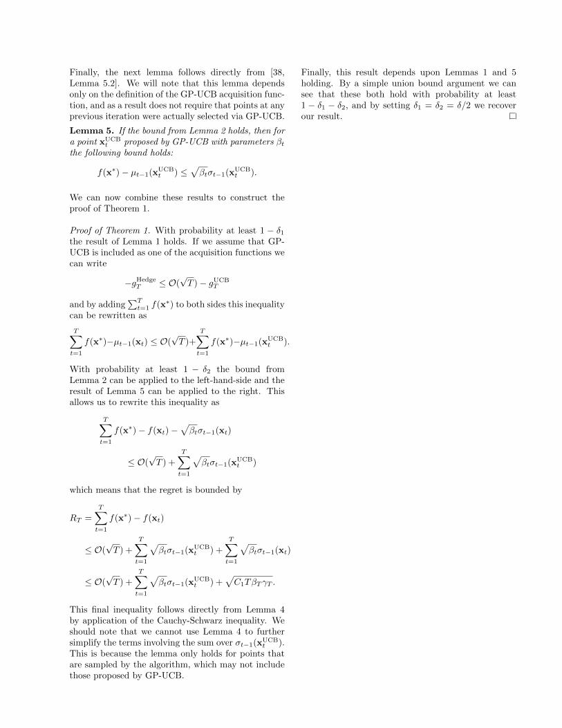
Finally, the next lemma follows directly from [38,Lemma 5.2]. We will note that this lemma dependsonly on the definition of the GP-UCB acquisition func-tion, and as a result does not require that points at anyprevious iteration were actually selected via GP-UCB.

Lemma 5. If the bound from Lemma 2 holds, then fora point xUCB

t proposed by GP-UCB with parameters βtthe following bound holds:

f(x∗)− µt−1(xUCBt ) ≤

√βtσt−1(xUCB

t ).

We can now combine these results to construct theproof of Theorem 1.

Proof of Theorem 1. With probability at least 1 − δ1the result of Lemma 1 holds. If we assume that GP-UCB is included as one of the acquisition functions wecan write

−gHedgeT ≤ O(

√T )− gUCB

T

and by adding∑T

t=1 f(x∗) to both sides this inequalitycan be rewritten as

T∑t=1

f(x∗)−µt−1(xt) ≤ O(√T )+

T∑t=1

f(x∗)−µt−1(xUCBt ).

With probability at least 1 − δ2 the bound fromLemma 2 can be applied to the left-hand-side and theresult of Lemma 5 can be applied to the right. Thisallows us to rewrite this inequality as

T∑t=1

f(x∗)− f(xt)−√βtσt−1(xt)

≤ O(√T ) +

T∑t=1

√βtσt−1(xUCB

t )

which means that the regret is bounded by

RT =

T∑t=1

f(x∗)− f(xt)

≤ O(√T ) +

T∑t=1

√βtσt−1(xUCB

t ) +

T∑t=1

√βtσt−1(xt)

≤ O(√T ) +

T∑t=1

√βtσt−1(xUCB

t ) +√C1TβT γT .

This final inequality follows directly from Lemma 4by application of the Cauchy-Schwarz inequality. Weshould note that we cannot use Lemma 4 to furthersimplify the terms involving the sum over σt−1(xUCB

t ).This is because the lemma only holds for points thatare sampled by the algorithm, which may not includethose proposed by GP-UCB.

Finally, this result depends upon Lemmas 1 and 5holding. By a simple union bound argument we cansee that these both hold with probability at least1 − δ1 − δ2, and by setting δ1 = δ2 = δ/2 we recoverour result.