Bayesian Depth-from-Defocus with Shading Constraints

Chen Li1 Shuochen Su3 Yasuyuki Matsushita2 Kun Zhou1 Stephen Lin2

1State Key Lab of CAD&CG, Zhejiang University 2Microsoft Research Asia 3Tsinghua University

Abstract

We present a method that enhances the performanceof depth-from-defocus (DFD) through the use of shadinginformation. DFD suffers from important limitations –namely coarse shape reconstruction and poor accuracy ontextureless surfaces – that can be overcome with the help ofshading. We integrate both forms of data within a Bayesianframework that capitalizes on their relative strengths. Shad-ing data, however, is challenging to recover accurately fromsurfaces that contain texture. To address this issue, we pro-pose an iterative technique that utilizes depth informationto improve shading estimation, which in turn is used to ele-vate depth estimation in the presence of textures. With thisapproach, we demonstrate improvements over existing DFDtechniques, as well as effective shape reconstruction of tex-tureless surfaces.

1. Introduction

Depth-from-defocus (DFD) is a widely-used techniquethat utilizes the relationship between depth, focus setting,and image blur to passively estimate a range map. A pairof images is typically acquired with different focus settings,and the differences between their local blur levels are thenused to infer the depth of each scene point. In contrast toactive sensing techniques such as 3D scanning, DFD doesnot require direct interaction with the scene. Additionally,it offers the convenience of employing a single stationarycamera, unlike methods based on stereo vision.

With the rising popularity of large format lenses for highresolution imaging, DFD may increase in application dueto the shallow depth of field of such lenses. However, thereexist imaging and scene factors that limit the estimation ac-curacy of DFD. Among these is the limited size of lens aper-tures, which leads to coarse depth resolution. In addition tothis, depth estimates can be severely degraded in areas withinsufficient scene texture for measuring local blur levels.

We present in this paper a technique that aims to mit-igate the aforementioned drawbacks of DFD through theuse of shading information. In contrast to defocus blur,shading not only indicates the general shape of a surface,

but also reveals high-frequency shape variations that allowshape-from-shading (SFS) methods to match or exceed thelevel of detail obtainable by active sensing [10, 32]. Wetherefore seek to capitalize on shading data to refine andcorrect the coarse depth maps obtained from DFD. Theutilization of shading in conjunction with DFD, however,poses a significant challenge in that the scene texture gener-ally needed for DFD interferes with the operation of shape-from-shading, which requires surfaces to be free of albedovariations. Moreover, DFD and SFS may produce incon-gruous depth estimates that need to be reconciled.

To address these problems, we first propose a Bayesianformulation of DFD that incorporates shading constraintsin a manner that locally emphasizes shading cues in areaswhere there are ambiguities in DFD. To enable the use ofshading constraints in textured scenes, this Bayesian DFDis combined in an iterative framework with a depth-guidedintrinsic image decomposition that aims to separate shad-ing from texture. These two components mutually ben-efit each other in the iterative framework, as better depthestimates lead to improvements in depth-guided decompo-sition, while more accurate shading/texture decompositionamends the shading constraints and thus results in betterdepth estimates.

In this work, the object surface is assumed to be Lamber-tian, and the illumination environment is captured by imag-ing a sphere with a known reflectance. Our experimentsdemonstrate that the performance of Bayesian DFD withshading constraints surpasses that of existing DFD tech-niques over both coarse and fine scales. In addition, the useof shading information allows our Bayesian DFD to workeffectively even for the case of untextured surfaces.

2. Related Work

Depth-from-defocus There exists a substantial amount ofliterature on DFD, beginning with works that handle objectswhose brightness consists of step edges [18, 25, 9]. Sincethe in-focus intensity profile of these edges is known, theirdepth can be determined from the edge blur. Later methodshave instead assumed that object surfaces can be locally ap-proximated by a plane parallel to the sensor [33, 26, 30],such that local depth variations can be disregarded in the

1

estimation. Some techniques utilize structured illuminationto deal with textureless surfaces and improve blur estima-tion [15, 14, 29]. DFD has been formulated as a Markovrandom field (MRF) problem, which allows inclusion ofconstraints among neighboring points [21, 22, 20]. Defo-cus has also been modeled as a diffusion process that doesnot require recovery of the in-focus image when estimatingdepth [6].

Shape-from-shading Considerable work has also beendone on shape-from-shading. We refer the reader to theSFS surveys in [34, 5], and review only the most rele-vant methods here. SFS has traditionally been applied un-der restrictive settings (e.g., Lambertian surfaces, uniformalbedo, directional lighting, orthographic projection), andseveral works have aimed to broaden its applicability, suchas to address perspective projection [19], non-Lambertianreflectance [16], and natural illumination [10, 8]. Non-uniform albedo has been particularly challenging to over-come, and has been approached using smoothness and en-tropy priors on reflectance [3]. Our work instead takes ad-vantage of defocus information to improve estimation fortextured surfaces. Shape-from-shading has also been usedto refine the depth data of uniform-albedo objects obtainedby multi-view stereo [32]. In our method, SFS is used in thecontext of DFD with scenes containing albedo variations.

Intrinsic images Intrinsic image decomposition aims toseparate an image into its reflectance and shading compo-nents. This is an ill-posed problem, since there are twiceas many unknowns (reflectance, shading) as observations(image intensities) per pixel. The various approaches thathave been employed make this problem tractable throughthe inclusion of additional constraints, such as those derivedfrom Retinex theory [11], trained classifiers [28], and mul-tiple images under different lighting conditions [31]. De-spite the existence of these different decomposition cues,the performance of intrinsic image algorithms has in gen-eral been rather limited [7]. Recently, range data has beenexploited to provide strong constraints for decomposition,and this has led to state-of-the-art results [12]. Inspired bythis work, we also utilize depth information to aid intrinsicimage decomposition. However, our setting is considerablymore challenging, since the depth information we start withis very rough, due to the coarse depth estimates of DFD andthe problems of SFS when textures are present.

3. ApproachIn this section, we present our method for Bayesian DFD

with shading constraints. We begin with a review of basicDFD principles, followed by a description of our BayesianDFD model, our shading-based prior term, the method for

Figure 1. Imaging model used in depth-from-defocus.

handling surface textures, and finally the iterative algorithmthat integrates all of these components.

3.1. Basic principles of DFD

DFD utilizes a pair of images taken with different focussettings. The effects of these focus settings on defocus blurwill be described in terms of the quantities shown in Fig. 1.Let us consider a scene point P located at a distance d fromthe camera lens. The light rays radiated from P to the cam-era are focused by the lens to a point Q according to the thinlens equation:

1

d+

1

vd=

1

F, (1)

where vd is the distance of Q from the lens, and F is thefocal length. When the focus setting v, which representsthe distance between the lens and sensor plane, is equal tovd, the rays of P converge onto a single point on the sensor,and P is thus in focus in the image. However, if v = vd, thefocused point Q does not lie on the sensor plane, and P thenappears blurred because its light is distributed to differentpoints on the sensor. Because of the rotational symmetry oflenses, this blur is in the form of a circle. The radius b ofthis blur circle can be geometrically derived as

b =Rv

2

∣∣∣∣ 1F − 1

v− 1

d

∣∣∣∣ , (2)

where R is the radius of lens. As seen from this equation,there is a direct relationship between depth d and blur radiusb for a given set of camera parameters.

The light intensity of P within the blur circle can be ex-pressed as a distribution function known as the point spreadfunction (PSF), which we denote by h. In this paper, wemodel the PSF h using a 2D Gaussian function [18]:

h(x, y;σ) =1

2πσ2e−

x2+y2

2σ2 (3)

with standard deviation σ = γb where the constant γ canbe determined by calibration [9]. Using the PSF, we can

2

express the irradiance I measured on the image plane as thefollowing convolution:

I(x, y) = If ∗ h(x, y, b), (4)

where If is the all-focused image of the scene, such as thatcaptured by a pinhole camera.

In DFD, we have two images, I1 and I2, which are cap-tured at the same camera position but with different focussettings, v1 and v2:

I1(x, y) = If ∗ h(x, y;σ1),I2(x, y) = If ∗ h(x, y;σ2),

(5)

where σ1 = γ ∗ b1 and σ2 = γ ∗ b2. Without loss of gener-ality, assume that σ1 < σ2. I2 can then be expressed as thefollowing convolution on I1

I2(x, y) = I1(x, y) ∗ h(x, y;∆σ), (6)

where ∆σ2 = σ22 −σ1

2. In the preceding equations, it canbe seen that the defocus difference, ∆σ, is determined bythe depth d and the two known focal settings v1 and v2, soEq. (6) can be represented as

I2(x, y) = I1(x, y) ∗ h(x, y, d), (7)

where d is the depth of pixel Px,y.Based on Eq. (7), most DFD algorithms solve for depth

by minimizing the following energy function or some vari-ant of it:

argmind

(I1(x, y) ∗ h(x, y, d)− I2(x, y))2. (8)

3.2. Bayesian depth­from­defocus model

We now formulate the DFD problem within a Bayesianframework and obtain a solution using a Markov ran-dom field (MRF). A basic review of Bayesian models andMarkov random fields can be found in [4, 17]. MRF-basedsolutions of DFD have also been used in [22, 20], and aBayesian analysis of the larger light-field problem was ad-dressed in [13].

Let i = 1, . . . , N index a 2D lattice G(ν, ε) of im-age pixels, where ν is the set of pixels and ε is the setof links between pixels in a 4-connected graph. In corre-spondence with G, let d = (d1, d2, .., dN ) denote values ofthe depth map D, and let I(1) = (I

(1)1 , I

(1)2 , . . . , I

(1)N ) and

I(2) = (I(2)1 , I

(2)2 , . . . , I

(2)N ) be the observations at the pix-

els. Depth estimation can then be formulated as a maximuma posteriori estimation problem, expressed using Bayes’theorem as follows:

d = argmaxd

P (d|I(1), I(2)) (9)

= argmaxd

P (I(1), I(2)|d)P (d)

= argmind

[L(I(1), I(2)|d) + L(d)

]

where P (d) is the prior distribution of depth map d,P (I(1), I(2)|d) is the likelihood of observations I(1), I(2),and L is the log likelihood of P , i.e. L = − logP .

The likelihood term can be modeled as the basic DFDenergy from Eq. (8), and the prior term as depth smoothnessalong the links [22]:

L(I(1), I(2)|d) =∑i∈ν

(I(1)i ∗ h(i, d)− I

(2)i )2, (10)

L(d) = λ∑

(i,j)∈ε

(di − dj)2. (11)

Hereafter, this particular formulation will be referred to asstandard DFD.

To optimize the MRF model of Eqs. (10)-(11), we usethe max-product variant of the belief propagation algo-rithm [27], with a message update schedule that propagatesmessages in one direction and updates each node immedi-ately.

3.3. Shading­based prior term

The smoothness prior of Eq. (11) can reduce noise inthe reconstructed depth, but does not provide any additionalknowledge about the scene. We propose to use a more in-formative prior based on the shading observed in the DFDimage pair, which is helpful both for reconstructing surfaceswith little texture content and for incorporating the fine-scale shape details that shading exhibits. In this section,we consider the case of uniform-albedo surfaces, for whichshading can be easily measured. The more complicated caseof textured surfaces will be addressed in Sections 3.4-3.5.

Lambertian shading can be modeled as a quadratic func-tion of the surface normal [23, 10]:

s(n) = nTMn, (12)

where nT = (nx, ny, nz, 1) for surface normal n, and M isa symmetric 4× 4 matrix that depends on the lighting envi-ronment. With this shading model, we solve for the surfacenormal of each pixel using the method in [10]. We alsoobtain the 3D coordinates for each point by re-projectingeach pixel into the scene according to its image coordinates(x, y), depth value d from DFD, and the perspective projec-tion model: ((

x− w

2

)ud,

(y − h

2

)ud, d

),

where w×h is the resolution of the image, and u is the pixelsize.

For each pair of linked pixels i, j in the MRF, we nowhave their depths di, dj , 3D positions pi,pj , and normalsni,nj . Since the vector −−→pipj should be perpendicular to

3

(a) (b) (c)Figure 2. Effect of different prior terms on DFD. (a) Original im-age (synthesized so that ground truth depth is available). (b/c)Close-up of depth estimates for the red/green box in (a). Fromtop to bottom: DFD with no prior, the smoothness prior, and theshading-based prior, followed by the ground truth depth.

the normal direction ni + nj , we formulate the shading-based prior term as

L(d) = λ∑

(i,j)∈ε

((pj − pi)

T ni + nj

∥ni + nj∥

)2

. (13)

where ε denotes the set of 4-connected neighbors over theMRF. DFD with this shading-based prior in place of thesmoothness prior will be referred to as DFD with shadingconstraints.

In the practical application of this shading constraint, wehave a pair of differently focused images from which to ob-tain the shading data. The most in-focus parts of the twoimages are combined into a single image by focal stack-ing using Microsoft Research’s Image Composite Editor(ICE) [1], which also automatically aligns different mag-nifications among the defocused images. This image is thenused for surface normal estimation, with the lighting en-vironment measured using a sphere placed in the scene asdone in [10].

As shown in Fig. 2, the incorporation of shading con-straints leads to improvements in DFD, especially in areaswith little intensity variation. Such areas have significantdepth ambiguity in DFD, because the likelihood energy inEq. (10) varies little with respect to estimated depth. In suchcases, DFD needs to rely on a prior term to obtain a distinctsolution. The simple smoothness prior of Eq. (11) helps byusing the depths of neighbors as a constraint, but this mayblur high frequency details. By contrast, the shape-basedprior term of Eq. (13) provides fine-scale shape informationthat more effectively resolves uncertainties in DFD.

3.4. Texture Handling

Shading information becomes considerably more diffi-cult to extract from an image when its surfaces contain tex-

ture. This problem arises because the brightness variationsfrom shading and texture are intertwined in the image inten-sities. To separate shading from texture, methods for intrin-sic image decomposition solve the following equation foreach pixel p:

ip = sp + rp, (14)

where i, s and r are respectively the logarithms of the imageintensity, shading value, and reflectance value.

In this paper, we decompose an image into its shadingand reflectance components with the help of shape infor-mation provided by DFD. The method we employ is basedon the work in [12], which uses streams of video and depthmaps captured by a moving Kinect camera. In contrast totheir work, we do not utilize temporal constraints on thedecomposition, since video streams are unavailable in oursetting. Also, we are working with depth data that is oftenof much lower quality.

The decomposition utilizes the conventional Retinexmodel with additional constraints on non-local re-flectance [24] and on similar shading among points thathave the same surface normal direction. Let Ω be the setof all pixels, ℵ be the set of 8-connected pixel pairs, Gr(p)be the set of pixels having a similar local texture pattern asp (computed as in [24]), and Gs(p) be the set of pixels withthe same surface normal as p. Then the shading componentof the image is computed through the following minimiza-tion:

argmins

∑(p,q)∈ℵ

[ωp,q

s(sp − sq)2 + ωp,q

r((ip − sp)− (iq − sq))2]

+∑p∈Ω

∑q∈Gr(p)

[ωnlr((ip − sp)− (iq − sq))

2]

+∑p∈Ω

∑q∈Gs(p)

[ωnls(sp − sq)

2], (15)

ωp,qr =

ωr if (1− cTp cq) < τr,0 otherwise

(16)

ωp,qs =

ωs if (1− nT

p nq) < τr,0.1ωs otherwise

(17)

where c denotes chromaticity, n denotes surface normal,and ωr, ωnlr, ωs and ωnls are coefficients that balance thelocal and non-local reflectance constraints, and local andnon-local shading constraints, respectively.

We note that Eq. (15) is a quadratic function which canbe simplified to a standard quadratic form:

argmins

1

2sT As− bT s+ c. (18)

It is optimized in our implementation using the precondi-tioned conjugate gradient algorithm.

4

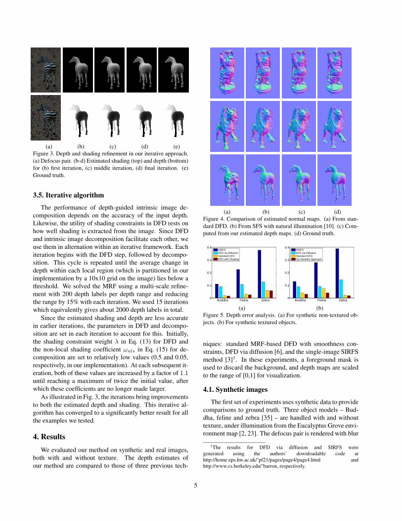
(a) (b) (c) (d) (e)Figure 3. Depth and shading refinement in our iterative approach.(a) Defocus pair. (b-d) Estimated shading (top) and depth (bottom)for (b) first iteration, (c) middle iteration, (d) final iteration. (e)Ground truth.

3.5. Iterative algorithm

The performance of depth-guided intrinsic image de-composition depends on the accuracy of the input depth.Likewise, the utility of shading constraints in DFD rests onhow well shading is extracted from the image. Since DFDand intrinsic image decomposition facilitate each other, weuse them in alternation within an iterative framework. Eachiteration begins with the DFD step, followed by decompo-sition. This cycle is repeated until the average change indepth within each local region (which is partitioned in ourimplementation by a 10x10 grid on the image) lies below athreshold. We solved the MRF using a multi-scale refine-ment with 200 depth labels per depth range and reducingthe range by 15% with each iteration. We used 15 iterationswhich equivalently gives about 2000 depth labels in total.

Since the estimated shading and depth are less accuratein earlier iterations, the parameters in DFD and decompo-sition are set in each iteration to account for this. Initially,the shading constraint weight λ in Eq. (13) for DFD andthe non-local shading coefficient ωnls in Eq. (15) for de-composition are set to relatively low values (0.5 and 0.05,respectively, in our implementation). At each subsequent it-eration, both of these values are increased by a factor of 1.1until reaching a maximum of twice the initial value, afterwhich these coefficients are no longer made larger.

As illustrated in Fig. 3, the iterations bring improvementsto both the estimated depth and shading. This iterative al-gorithm has converged to a significantly better result for allthe examples we tested.

4. ResultsWe evaluated our method on synthetic and real images,

both with and without texture. The depth estimates ofour method are compared to those of three previous tech-

(a) (b) (c) (d)Figure 4. Comparison of estimated normal maps. (a) From stan-dard DFD. (b) From SFS with natural illumination [10]. (c) Com-puted from our estimated depth maps. (d) Ground truth.

Buddha Feline Zebra0

0.1

0.2

0.3

0.4

SIRFSDFD via DiffusionStandard DFDDFD with Shading

Buddha Feline Zebra0

0.1

0.2

0.3

0.4

SIRFSDFD via DiffusionStandard DFDOur Iterative Approach

(a) (b)Figure 5. Depth error analysis. (a) For synthetic non-textured ob-jects. (b) For synthetic textured objects.

niques: standard MRF-based DFD with smoothness con-straints, DFD via diffusion [6], and the single-image SIRFSmethod [3]1. In these experiments, a foreground mask isused to discard the background, and depth maps are scaledto the range of [0,1] for visualization.

4.1. Synthetic images

The first set of experiments uses synthetic data to providecomparisons to ground truth. Three object models – Bud-dha, feline and zebra [35] – are handled with and withouttexture, under illumination from the Eucalyptus Grove envi-ronment map [2, 23]. The defocus pair is rendered with blur

1The results for DFD via diffusion and SIRFS weregenerated using the authors’ downloadable code athttp://home.eps.hw.ac.uk/˜pf21/pages/page4/page4.html andhttp://www.cs.berkeley.edu/˜barron, respectively.

5

(a) (b) (c) (d) (e) (f) (g) (h) (i) (j) (k)Non-texture results Texture results

Figure 6. Synthetic data results. (a) Ground truth depth maps. (b/g) Non-textured/textured input defocus pairs. Depth estimate results for(c/h) SIRFS [3], (d/i) DFD via diffusion [6], (e/j) standard DFD, (f/k) our method.

according to Eq. (2) and with the virtual camera parametersset to F = 0.01, Fnum = 2.0, and γ = 1000000. Thetwo focal settings are chosen such that their focal planesbound the ground truth depth map, and random Gaussiannoise with a standard deviation of 1.0 is added to simulatereal images.

The benefits of utilizing shading information with DFDare illustrated in Fig. 4 for normal map estimation on tex-tureless objects. Here, the normal maps are constructedfrom gradients in the estimated depth maps. The uncertaintyof DFD in areas with little brightness variation is shownto be resolved by the shading constraints. As we use themethod of SFS with natural illumination [10] to obtain sur-face normals, our technique is able to recover a similar levelof shape detail.

Our depth estimation results are exhibited together withthose of the comparison techniques in Fig. 6. The aver-age errors for each method within the foreground masks areshown in Fig. 52. With the information in a defocus pair,our method can obtain results more reliable than that of the

2DFD by diffusion does not work as well as standard DFD on our ob-jects because its preconditioning is less effective when the intensity varia-tions are not large.

single-image SIRFS technique. In comparison to the twoDFD methods, ours is able to recover greater shape detailthrough the use of shading.

4.2. Real images

We also compared our method to related techniques us-ing real images. As with the synthetic data, the comparisonmethods are SIRFS [3], DFD via diffusion [6], and standardDFD. The images were captured using a Canon 5D Mark IIcamera with a 100mm lens. We mounted the camera on atripod and shot the images in RAW mode with the objectsabout 50cm away.

In order to use our shading constraints, we first calibratethe natural illumination using a white Lambertian sphere,and then use the known surface normals of the sphere tosolve the shading matrix in Eq. (12) by least-squares opti-mization. Because the albedo of the sphere may differ fromthose of our target objects, we estimate the relative albedobetween target objects and the sphere simply by comparingthe brightness of manually identified local areas that have asimilar normal orientation. For objects with surface texture,the albedo of the local area used in this comparison is usedas the reference albedo for the object.

6

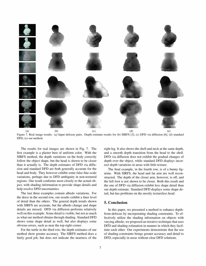
(a) (b) (c) (d) (e)Figure 7. Real image results. (a) Input defocus pairs. Depth estimate results for (b) SIRFS [3], (c) DFD via diffusion [6], (d) standardDFD, (e) our method.

The results for real images are shown in Fig. 7. Thefirst example is a plaster bust of uniform color. With theSIRFS method, the depth variations on the body correctlyfollow the object shape, but the head is shown to be closerthan it actually is. The depth estimates of DFD via diffu-sion and standard DFD are both generally accurate for thehead and body. They however exhibit some false fine-scalevariations, perhaps due to DFD ambiguity in non-texturedregions. Our result conforms most closely to the actual ob-ject, with shading information to provide shape details andhelp resolve DFD uncertainties.

The last three examples contain albedo variations. Forthe dress in the second row, our results exhibit a finer levelof detail than the others. The general depth trends shownwith SIRFS are accurate, but the albedo change and shapedetails are missed. DFD via diffusion performs relativelywell on this example. Some detail is visible, but not as muchas what our method obtains through shading. Standard DFDshows some shape detail as well, but also displays someobvious errors, such as near the top-right corner.

For the turtle in the third row, the depth estimates of ourmethod show greater accuracy. The SIRFS method does afairly good job, but does not indicate the nearness of the

right leg. It also shows the shell and neck at the same depth,and a smooth depth transition from the head to the shell.DFD via diffusion does not exhibit the gradual changes ofdepth over the object, while standard DFD displays incor-rect depth variations in areas with little texture.

The final example, in the fourth row, is of a bunny fig-urine. With SIRFS, the head and far arm are well recon-structed. The depth of the closer arm, however, is off, andthe left foot is not shown to be closer. Both this result andthe one of DFD via diffusion exhibit less shape detail thanour depth estimate. Standard DFD displays some shape de-tail, but has problems on the mostly textureless head.

5. Conclusion

In this paper, we presented a method to enhance depth-from-defocus by incorporating shading constraints. To ef-fectively utilize the shading information on objects withvarying albedo, we proposed an iterative technique that usesDFD and shading estimation in manner in which they facil-itate each other. Our experiments demonstrate that the useof shading constraints brings greater accuracy and detail toDFD, especially in areas without clear DFD solutions.

7

In future work, we plan to investigate ways to increasethe accuracy of our depth estimates. Our current implemen-tation assumes the incident illumination to be the same at allsurface points. However, this will not be the case due to dif-ferent self-occlusions of an object towards different lightingdirections. This issue could be addressed by computing thelight visibility of each point from the estimated depth.

AcknowledgementsThis work was partially supported by NSFC (No.

61272305). It was done while Chen Li and Shuochen Suwere visiting students at Microsoft Research Asia.

References[1] Image composite editor. http://research.microsoft.com/

en-us/um/redmond/groups/ivm/ice.[2] Light probe image gallery.

http://www.pauldebevec.com/Probes/.[3] J. T. Barron and J. Malik. Color constancy, intrinsic images,

and shape estimation. In ECCV, 2012.[4] A. Blake, P. Kohli, and C. Rother. Markov Random Fields

for Vision and Image Processing. The MIT Press, 2011.[5] J.-D. Durou, M. Falcone, and M. Sagona. Numerical meth-

ods for shape-from-shading: A new survey with benchmarks.Compt. Vision and Image Underst., 109(1):22–43, 2008.

[6] P. Favaro, S. Soatto, M. Burger, and S. Osher. Shape fromdefocus via diffusion. IEEE Trans. Patt. Anal. and Mach.Intel., 30(3):518–531, 2008.

[7] R. Grosse, M. K. Johnson, E. H. Adelson, and W. T. Free-man. Ground truth dataset and baseline evaluations for in-trinsic image algorithms. In ICCV, 2009.

[8] R. Huang and W. Smith. Shape-from-shading under complexnatural illumination. In ICIP, pages 13–16, 2011.

[9] T.-l. Hwang, J. Clark, and A. Yuille. A depth recovery algo-rithm using defocus information. In CVPR, pages 476 –482,jun 1989.

[10] M. K. Johnson and E. H. Adelson. Shape estimation in nat-ural illumination. In CVPR, pages 2553–2560, 2011.

[11] R. Kimmel, M. Elad, D. Shaked, R. Keshet, and I. Sobel. Avariational framework for retinex. Int. Journal of ComputerVision, 52:7–23, 2003.

[12] K. J. Lee, Q. Zhao, X. Tong, M. Gong, S. Izadi, S. U. Lee,P. Tan, and S. Lin. Estimation of intrinsic image sequencesfrom image+depth video. In ECCV, pages 327–340, 2012.

[13] A. Levin, W. T. Freeman, and F. Durand. Understandingcamera trade-offs through a bayesian analysis of light fieldprojections. In ECCV, pages 88–101, 2008.

[14] S. Nayar, M. Watanabe, and M. Noguchi. Real-time focusrange sensor. In ICCV, pages 995 –1001, jun 1995.

[15] M. Noguchi and S. Nayar. Microscopic shape from focususing active illumination. In ICPR, volume 1, pages 147–152, oct 1994.

[16] G. Oxholm and K. Nishino. Shape and reflectance from nat-ural illumination. In ECCV, pages I:528–541, 2012.

[17] B. Peacock, N. Hastings, and M. Evans. Statistical Distribu-tions. Wiley-Interscience, June 2000.

[18] A. P. Pentland. A new sense for depth of field. IEEE Trans.Patt. Anal. and Mach. Intel., 9(4):523–531, Apr. 1987.

[19] E. Prados and O. Faugeras. A generic and provably conver-gent shape-from-shading method for orthographic and pin-hole cameras. Int. Journal of Computer Vision, 65(1):97–125, 2005.

[20] A. Rajagopalan, S. Chaudhuri, and U. Mudenagudi. Depthestimation and image restoration using defocused stereopairs. IEEE Trans. Patt. Anal. and Mach. Intel., 26(11):1521–1525, nov. 2004.

[21] A. N. Rajagopalan and S. Chaudhuri. Optimal selection ofcamera parameters for recovery of depth from defocused im-ages. In CVPR, 1997.

[22] A. N. Rajagopalan and S. Chaudhuri. An mrf model-basedapproach to simultaneous recovery of depth and restorationfrom defocused images. IEEE Trans. Patt. Anal. and Mach.Intel., 21(7):577–589, July 1999.

[23] R. Ramamoorthi and P. Hanrahan. An efficient representa-tion for irradiance environment maps. In ACM SIGGRAPH,pages 497–500, 2001.

[24] L. Shen, P. Tan, and S. Lin. Intrinsic image decompositionwith non-local texture cues. In CVPR, pages 1 –7, june 2008.

[25] M. Subbarao and N. Gurumoorthy. Depth recovery fromblurred edges. In CVPR, pages 498 –503, jun 1988.

[26] M. Subbarao and G. Surya. Depth from defocus: A spa-tial domain approach. Int. Journal of Computer Vision,13(3):271–294, 1994.

[27] R. Szeliski, R. Zabih, D. Scharstein, O. Veksler, V. Kol-mogorov, A. Agarwala, M. Tappen, and C. Rother. A com-parative study of energy minimization methods for markovrandom fields with smoothness-based priors. IEEE Trans.Patt. Anal. and Mach. Intel., 30(6):1068 –1080, june 2008.

[28] M. F. Tappen, E. H. Adelson, and W. T. Freeman. Estimatingintrinsic component images using non-linear regression. InCVPR, pages 1992–1999, 2006.

[29] M. Watanabe, S. Nayar, and M. Noguchi. Real-Time Com-putation of Depth from Defocus. In Proc. SPIE, volume2599, pages 14–25, Jan 1996.

[30] M. Watanabe and S. K. Nayar. Rational filters for pas-sive depth from defocus. Int. Journal of Computer Vision,27(3):203–225, May 1998.

[31] Y. Weiss. Deriving intrinsic images from image sequences.In ICCV, pages 68–75, 2001.

[32] C. Wu, B. Wilburn, Y. Matsushita, and C. Theobalt. High-quality shape from multi-view stereo and shading under gen-eral illumination. In CVPR, pages 969–976, 2011.

[33] Y. Xiong and S. A. Shafer. Depth from focusing and defo-cusing. In CVPR, pages 68–73, 1993.

[34] R. Zhang, P.-S. Tsai, J. Cryer, and M. Shah. Shape-from-shading: a survey. IEEE Trans. Patt. Anal. and Mach. Intel.,21(8):690 –706, aug 1999.

[35] K. Zhou, X. Wang, Y. Tong, M. Desbrun, B. Guo, and H.-Y.Shum. Texturemontage: Seamless texturing of arbitrary sur-faces from multiple images. ACM Transactions on Graphics,24(3):1148–1155, 2005.

8