Lab Report:Investigating Jumping Spider Vision

Aleke NolteSupervisors: Dr. Tom Gheysens

Dr. Daniel HennesProf. Dr. sc. nat. Verena V. Hafner

February 9, 2015

Abstract

Jumping spiders are capable of estimating the distance to theirprey relying only on the information from one of their main eyes.Recently it has been suggested that jumping spiders perform this es-timation based on image defocus cues. In oder to gain insight into themechanisms involved in this blur-to-distance mapping as performedby the spider and to judge whether inspirations can be drawn fromspider vision for Depth-from-Defocus computer vision algorithms, wemodel the relevant spider eye with the 3D software Blender and ren-der scenes how the spider would see them. We test a simple andwell known Depth-from-Defocus algorithm on this dataset and showwhy it is not capable of estimating distances correctly. We concludethat our model is too abstract to allow inferences to be drawn aboutthe spider’s Depth-from-Defocus mechanism. Further we propose an-other straightforward way to quantify defocus and suggest additionalaspects to be included in the model.

1 Introduction

Computer Vision (CV) algorithms that deduce distances from two or moredefocussed images of a scene, so called Depth-from-Defocus (DFD) algo-rithms, have first been introduced in the late 1980s and the beginning of the1990s (e.g [1, 2]) and have been build upon subsequently to increase perfor-mance and robustness (e.g. [3]).Recently, Nagata et al. [4] presented a study which provides strong evidencethat jumping spiders also judge the distance to their prey based on defocuscues. In the first part of this study, all but one of the spider’s front facing

1

anterior median (AM) eyes were occluded. The spider was then presenteda fruit fly at different distances and jumping accuracy during hunting wasaccessed. It was found that there is no significant difference in performanceto an unblinded spider, indicating that the spider relies on monocular cuesfrom the AM eyes for distance estimation. What is special about the AMeye is that the photoreceptor cells are distributed over four layers, of whichthe two bottommost layers, Layer 1 (L1) and Layer 2 (L2) yield the input forthe DFD estimation: images projected onto the retina are blurry on L2 andsharp on L1 (Figure 2). Using the achromatic aberrations of the eye’s lensin the second part of their study (more details in Section 1.1), Nagata et alshow that the amount of blur on these layers indeed influences the jumpingdistance.The question now arises if both CV-DFD algorithms and the spider DFDmechanism are based on the same high level principles and if not, if CV-DFDalgorithms can be improved by learning from the spider’s DFD mechanism.Particularly interesting is that the spider achieves an apparently very accu-rate depth estimation with very simple components: A single lens and veryfew photoreceptors (e.g. an AM eye of the spider species Metaphidippus ae-neolus only has about 1200 photoreceptors in total [5]).A DFD sensor build of such basic components would be of great interestfor use in space: If only basic components are needed the sensor is likelyto be low in cost. Low cost equipment is highly suitable for simple space-crafts like cubesats, and an optical distance sensor would be advantageousfor formation flying and other types of swarm behaviour. A low cost opti-cal distance sensor would also be of use in debris removal, during dockingand landing and as a general fall-back or assisting option for other distancesensing equipment such as laser detection and ranging systems (LADAR),sound navigation and ranging systems (SONAR) and stereo vision systems.Furthermore a system consisting essentially of only lenses and sensors and nomechanical parts would be less fault-prone and lower in power consumptionthan above mentioned methods.In this work we take the first steps in investigating if spider vision has thepotential to advance such a vision sensor. To this end, we create a model ofthe anterior median (AM) eye of spider species Metaphiddipus aeneolus tosee what kind of images are created on the spider retina. Simply put, wewant to show “what the spider sees”. We then test a well known but basicDFD-algorithm [2] on these images to see if the spider’s depth assessmentperformance can be explained by the principles of this algorithm.

This paper is structured as follows: In the next Section 1.1 we describe themorphology of the AM eye of M. aeneolus as found by Land [5] and presentthe study above mentioned by Nagata et al. in more detail. In Section 2 we

2

specify the abstractions made and the modeling choices for our model of thespider eye in the 3D graphics software Blender [6]. Section 4 describes theDFD algorithm used and Section 5 delineates the datasets constructed andthe experiments performed, as well as an investigation on why the algorithmfails to perform on our spider datasets. The paper closes with a discussion onfurther elements to be included in the model and a simple possible alternativeto the algorithm used.

1.1 The anterior median spider eye

The photoreceptors of the retina of the AM eyes of the jumping spider aredistributed over four layers (see Figure 3). According to an analysis by Landfrom 1969 [5] the two topmost layers always receive defocussed images, asthe corresponding conjugate object planes lie behind, and not in front of thespider’s head. Recently, the two bottommost layers have been found to beessential for the judgement of distances: Nagata et al. found that these lay-ers contain mostly green light sensitive photo receptors and have shown inan experiment that a jumping spider performs accurate jumps when viewingtargets in green, but not in red light.Furthermore, they showed that the spiders consistently jumped to short inred light, thus underestimating the distance to their prey. Nagata et al.found that due to achromatic aberrations of the spider eye’s lens an objectviewed in red light results in the same amount of blur on the second retinalayer (L2) as the same object at a closer distance when viewed in green light(see Figure 2). Thus the underestimation of the distance to the prey in redlight is strong evidence that the spider judges the distance on defocus cues.

Morphology The anterior median spider eye resembles a long tube (Fig-ure 1), with the very curved cornea on one end and a boomerang shaped fourlayer retina on the other end (Figure 4). The four retina layers extend over arange of ca 50µm with the distances between layers and layer thicknesses asindicated in Figure 3. On the retina, the receptors are arranged in a hexag-onal lattice, with denser spacing closer to the optical axis and a more coarsespacing towards the periphery. The spacing in L2 is overall more coarse thanin L1, the minimum receptor spacing found in L1 is 1.7µm.

2 Modeling the Spider Eye

We model the AM eye of M. aeneolus with the help of the 3D graphicssoftware Blender [6]. To achieve physically accurate results of how light

3

Figure 1: Example shapes of jumping spider eyes. The anterior medianeyes (red arrows) resemble a long tube with a very curved cornea in thefront. http://tolweb.org/accessory/Jumping_Spider_Vision?acc_id=

1946, retrieved (12/15/2014)

Figure 2: Objects at distances d in red light and d′ in green light result inthe same amount of blur on Layer 2. (Figure taken from [4].)

4

Top L1

bottom L1

bottom L2

top L2

middle L1

x x

y

z

Figure 3: Arrangement of photoreceptor layers of M. aeneolus ’s retina. Lightfrom the lens enters the figure from the top. The bar on the right indicatesthe object distances that are conjugate to horizontal planes on the retina.The red line highlights the location of the focal plane. The legend on theleft indicates the location of the image planes used in our dataset. (Figureslightly modified from [5] to improve clarity).

is refracted through lens and posterior chamber we choose LuxRender 1, aphysically based rendering engine for the ray tracing part in place of Blender’sbuild-in Cycles engine. Cycles does not model glass well and is thus lesssuitable for an optical model, while LuxRender traces light according tomathematical models based on physical phenomena and is thus more suitable.In oder to facilitate the handling of the model, all used values are scaled bya factor of 10000.

Modeling lens and posterior chamber In our model the eye is rep-resented by a thick lens (r1 = 217µm, r2 = −525µm, d = 236µm) withrefractive index n = 1.412, enclosed by a black tube 3.The posterior chamber of the eye is modeled by setting the refractive indexof the back of the lens to that of spider ringer, i.e., n = 1.3354. Apertureand specific shape of the lens (see Figure 6) are achieved by creating a black

1http://www.luxrender.net, retrieved 06 January 20152LuxRender glass2 volume with corresponding refractive index3LuxRender matte material4LuxRender glass2 volume with corresponding refractive index

5

Figure 4: Boomerang shaped receptor grids of Layer 1 (left) and Layer 2(middle). The rightmost subfigure shows the receptors for Layer 3 and Layer4 superimposed. The crosses indicate the location where the layers wouldstack onto each other. For both Layer 1 and Layer 2 receptors are spacedmore densely along the optical axis and more coarsely in the periphery. Theminimal receptor spacing in Layer 1 is 1.7µm. (Figure taken from [5]).

torus5 with diameter d = 200µm at narrowest point. The resulting modelis shown in Figure 5. All the measurement values mentioned above are thesame as provided in [5] and summarised in Table 1.

Modeling receptor layers / sensor spacing For simplicity, we do notmodel the receptor layers as volumes (Figure 3), but simply as 2-dimensionalsensor planes. A sensor plane is realized in Blender by creating a plane oftranslucent material (to act as a “film”) and placing an orthogonal scenecamera behind it to record the image on the film. We record images atlocations of the sensor plane in z-axis corresponding to: The top of L2, thefocal plane (which coincides with the bottom of L2), the top of L1, themiddle of L1 and the bottom of L1. The corresponding back focal distances(BFD) are 450µm, 459µm, 464µm, 474µm and 485µm, respectively. In oursetup, we choose a quadratic film size and base the number of receptors (=

5LuxRender matte material

6

Figure 5: Blender model of the AM eye of M. aeneolus. The lens is a LuxRen-der glass2 volume with refractive index n = 1.41, the posterior chamber is aLuxRender glass2 volume with refractive index n = 1.335. The sensor is ofLuxRender translucent material. All other materials are of type LuxRendermatte and of black color to absorb light.

Eye Parameters

r1 −r2 d nlens npostr chamber f

217µm 525µm 236µm 1.41 1.355 504µm

Table 1: Parameters of the AM eye of M. aeneolus.

pixels) on the closest spacing in L1, resulting in a 117px× 177px film of size200µm× 200µm to approximate the receptors of a layer. We use this film torecord images for L1 as well as for L2. Even though the structure of the actualreceptor layers is boomerang shaped and only measures a few micrometers atits most narrow point, we assume that the spider can emulate a larger retinaby moving the retina in x-y direction, assumingly “stitching” the partialimages together to form a larger image. This behaviour might also result inhigher visual accuracy, emulating a more dense receptor spacing. We thusappropriately assume to model the retina as a square. To account for thepossible higher accuracy, we also create a parallel dataset with 370px×370pxoccupying the 200µm× 200µm sized film.

7

Sideview of lens in Blender model

x

y

z

Figure 6: Comparison of AM eye lens shape of M. aeneolus in the Blendermodel (left) with the lens shape as reported by Land (right, image takenfrom [5])

3 Dataset

We generate the spider dataset by rendering four different images (“objects”)as viewed through the spider eye, two artificial and two “natural” ones (seeFigure 7). The artificial ones are a checkerboard texture, where the sizeof one square corresponds to the size of a fruit fly (approx. 5 mm) anda black circle in front of a neutral background. Here, the diameter of thecircle also corresponded to 5mm. The artificial textures where chosen likethis to a) be able to visually judge the defocus around edges and b) get animpression how the size of prey on the sensor changes for different distancesfrom spider to prey. These textures however have a low frequency contentand lack detail. The DFD algorithm is reported to not perform well with low-frequency content images [2]. To account for this we include two additionalnatural images. It should be noted that even though these images displaya jumping spider and a fruit fly, these are not to scale, but much largerthan their real counterparts. Considering the possibility that the effectiveresolution of the spider eye is higher due to eye movement, we also create aset of higher resolution (370px × 370px) renderings for the natural images.We render images for each object placed at distances D = {1.5, 3 and 6cm}from the lens. These distances approximately correspond to the conjugateplanes (in object space) of the Bottom of L1, the middle of L1 and the topof L1, respectively and are chosen so to ensure that “good” images , i.e.

8

Figure 7: Images used to generate the spider dataset. Theseare the “objects” that are placed in front of the lens to beviewed through the lens. (Spider image from http://commons.

wikimedia.org/wiki/File:Female_Jumping_Spider_-_Phidippus_

regius_-_Florida.jpg, retrieved 04/01/2014; fruit fly imagefrom http://www.carolina.com/drosophila-fruit-fly-genetics/

drosophila-living-ebony-chromosome-3-mutant/172500.pr, retrieved14/01/2014.

images with least amount of blur, are part of the dataset. Examples fromthe datasets are show in Figure 8.

4 Depth from Defocus Algorithm

In the following we will present the reasoning underlying DFD algorithmsand describe a basic algorithm as proposed by Subbarao in 1988 [2]. Eventhough the algorithm has been improved upon in many ways since it was firstproposed (e.g. [3]), most improvements address the image overlap problem- the problem that when segmenting an image into patches to estimate thedistance of each patch, each patch is influenced by objects in neighboringpatches due to the spread of the defocus. In our setup however, the objectswe consider are planes perpendicular to the optical axis so that the distancesare constant over the whole image. Accordingly these improvements are notexpected to increase the performance in our scenario, so that we only use theoriginal algorithm.

4.1 Subbarao’s DFD algorithm

If an object is not in focus, the amount of blur in the image can provideinformation about the distance of the object. Given that we know the cam-era’s parameters (focal length f , aperture A and the lens to sensor distancev) we can calculate the distance by basic geometry and Gauss’ lens formula.Gauss equation assumes a thin lens and relates the object distance and the

9

Top L2

Bottom L2

Top L1

Middle L1

Bottom L1

natural object artificial object

6cm 3cm 1.5cm 6cm 3cm 1.5cm

Figure 8: Examples for one natural and one artificial texture dataset. Shownare images at the sensor planes corresponding to Top of L2, bottom of L2,top of L1, middle of L1 and bottom of L1 (top to bottom) for object distancescorresponding to 6cm, 3cm and 1.5cm, (left to right). The red squares indi-cate the images that should be least blurry according to Gauss’ lens equation(Eq. 1).

focal length of the lens to the distance of the focussed image:

1

f=

1

D+

1

v, (1)

where D is the distance of the object to the lens.The diameter d of the blur circle is related to the other camera parameters

d = Av (1

f− 1

D− 1

v) , (2)

and the actual observed blur circle radius σ then depends on the cameraconstant ρ (which depends in parts on the pixel resolution and in part onother camera properties)

σ =ρ

2d . (3)

If the diameter of the blur circle is known Eq. (2) can easily be solved forobject distance D. Accordingly, the basis of most DFD algorithms including

10

Subbaraos’s algorithm, is the estimation of blur from two or more defocussedimages.The basic premise of the algorithm is that an out of focus image can becreated from a sharp image by convolving the sharp image with a pointspread function (PSF) that corresponds to the blur. For simplicity the PSFis often assumed to be a two dimensional Gaussian

h(x, y) =1

2πσ2e−

x2+y2

2σ2 (4)

with spread parameter σ. A blurred image g(x, y) can thus be obtained froma sharp image f(x, y) by convolving the sharp image with the PSF

g(x, y) = h(x, y) ∗ f(x, y) . (5)

Convolution in the spatial domain corresponds to multiplication in the fre-quency domain. Thus, when considering the blurry images in the frequencydomain we can eliminate the need for a sharp image:

Gk(ω, ν) = Hk(ω, ν)Fk(ω, ν)

G1(ω, ν)

G2(ω, ν)=H1(ω, ν)

H2(ω, ν).

Using the frequency space representation of Eq. (4) this leads to

H1(ω, ν)

H2(ω, ν)= exp

(−1

2(ω2 + ν2)(σ2

1 − σ22)

). (6)

Considering the power density spectra P (ω, ν) of the transform and rear-ranging allows to extract the relative defocus

σ21 − σ2

2 =−2

ω2 + ν2log

P1(ω, ν)

P2(ω, ν). (7)

In order to obtain a more robust estimation, the relative defocus is averagedover a region in frequency space

C =1

N

∑ω

∑ν

−2

ω2 + ν2log

P1(ω, ν)

p2(ω, ν), (8)

where P1(ω, ν) 6= P2(ω, ν) and N the number of frequency samples.It is then possible to solve for the blur of one of the images, e.g. σ2, bysolving the following quadratic equation:

(α2 − 1)σ22 + 2αβσ2 + β2 = C (9)

11

withα =

v1v2

(10)

and

β = ρv1A

2(

1

v2− 1

v1) . (11)

Using the obtained σ2 in Eq. 3 and Eq. 2 allows to solve for the distance D.

5 Experiments

5.1 Pre-experiment on kixor dataset

To test the functionality of the algorithm we first tested it on a small dataset6

of defocussed images obtained with an off the shelf camera. The dataset doesnot contain the exact distances of the objects pictured, nor does it include theexact lens to sensor distances but instead it reports the distance the camerafocusses on. Using Gauss’ lens formula, and by visually determining whichpart of the image is sharp, both u and D can be approximated. Testing thealgorithm on this dataset yields results in the correct order of magnitude ifthe blur in the images is not too high. The exact results also depend on thefrequencies used to calculate C. Examples are shown in Figure 9.

5.2 Experiments on spider dataset

Testing the algorithm on the spider data did not give consistent results. Formost object- and sensor distances, the estimated distance was neither in theright order of magnitude, nor did it reflect the ordering of distances (givinghigher estimates to objects further away and lower estimates to objects thatwere closer).

Figure 10 shows the estimates given by the algorithm for different objectdistances and for the different spider datasets.

In the following we analyse why the algorithm performs poorly on thespider datasets.

5.2.1 Misleading frequency content

As described in Section 4.1 the estimation of the blur of the images is basedon the “difference” of the two images in the frequency domain. Accordingly,if there is not enough or misleading frequency information in the image, thealgorithm is not expected to work. To address this we test the algorithm

6http://www.kixor.net/school/2008spring/comp776/project/results/, re-trieved 16/12/2014

12

Figure 9: Image patches extracted from kixor dataset. Shown are threeexamples of defocussed image pairs and the estimated as well as the actualdistances of the objects.

13

Figure 10: Depth estimates for the low resolution (117px × 117px) spiderdataset. Results are shown for a subset of pairings from image planes in L2and L1. The highlighted subfigure is the pairing that is assumed in spiders.

Figure 11: Depth estimates for the high resolution (370px × 370px) spiderdataset. Results are shown for a subset of pairings from image planes in L2and L1. The highlighted subfigure is the pairing that is assumed in spiders.

14

Figure 12: Amount of noise for different rendering times. Left: 1000 samplesper pixel, right: 10000 samples per pixel. Images are taken from the highresolution dataset 370px× 370px)

on a dataset with low frequency and normal frequency content (checkers,circle and ”natural image” dataset). The performance on the natural imagedataset is qualitatively the same as on the artificial datasets, indicating thatthe low frequency content of the image is not the reason for the failure.Also, the receptor grid is quite coarse (117px × 117px) so that fine detailswhich could provide valuable blurred edges (and with that more frequencyinformation) might not be captured. However, the algorithm’s performancedoes not increase on the high resolution natural images dataset (370px ×370px) (Figure 11).

Image noise levels The test datasets contain some noise due to the ren-dering process. During rendering, light paths are traced from Blender’s lightsource to the viewed object, through the lens, and onto the film. Each foundpath is called “a sample”. The process of rendering is computationally costlyand thus the numbers of samples per pixel (spp) is limited to 1000 in ouroriginal dataset. As shown in the left of Figure 12, the resulting image isslightly noisy. The noise is the same for different object distances, and thusthe frequencies corresponding to the noise are the same for both images,which in turn can influence the blur estimate.We test the algorithm on datasets with lower amounts of noise: on low passfiltered versions of the original dataset and a dataset with spp = 10000. (Fig-ure 12 right). The results of the algorithm remain qualitatively the same asshown in Figures 10 and 11. Accordingly, neither the rendering noise nor

15

the resolution of the images are the reason for the poor performance of thealgorithm.

5.2.2 Focal lengths

The focal length for M. aeneolus as measured by Land is 512µm, while thecalculated focal length for a thin lens in air and water amounts to 504µm.Using the above (Section 2) lens parameters (refractive indices, radii of cur-vature and thickness of the lens) allows to calculate the back focal length ofthe lens (BFL), that is the distance between the back of the lens and thefocal point, which amounts to 459µm. However, these calculations do nottake spherical aberrations into account. Due to spherical aberrations an im-age formed by a very curved lens may still be blurry, even though accordingto Gauss’ lens formula it should be in focus. The sensor distance for “best”focus is then the distance at which the “circle of confusion” is smallest.When setting up the sublayers for L1 and L2 relative to BFL = 459µm, theexpected trajectory from defocussed to focussed and back to defocused couldnot be observed in our renderings (Figure 8).

Taking into account that Land’s description of the eye may not be com-plete and to investigate a case that is closer to the considerations presentedby Nagata [4] (more clearly focussed and defocussed images) we create anadditional set of test images with sensor layer distances relative to the “best”focus, namely the BFL400 -dataset. We determined the best focus with thehelp of the autofocus function of the commercial optical software Zemax 7.Unlike in the ideal lens calculations Zemax’s autofocus function calculatesthe back focal length based on the smallest circle of confusion, resulting in aBFL of 400µm.For the layers placed relative to this value, a different blur profile can be ob-served (Figure 13). However, testing the algorithm on this dataset results inqualitatively the same performance as the mentioned experiments. This in-dicates that the poor performance of the algorithm is not due to an incorrectvalue for the focal length.

5.2.3 Reverse calculations: Which values of σ and C would weexpect?

In order to further investigate why the algorithm performs poorly on the spi-der dataset, we calculate the values for C and σ which the algorithm wouldexpect in order to yield the correct results. Figure 14 shows a comparison ofthe calculated values for C and the values for C obtained by using the imagesfrom the spider dataset in Eq 8, f = 459µm and D ∈ {1.5cm, 3cm, 6cm}. It

7https://www.zemax.com

16

Top L2 (BFD= 391μm)

Bottom L2 (BFD= 400μm)

Top L1 (BFD= 405μm)

Middle L1 (BFD= 415μm)

Bottom L1 (BFD= 425μm)

object distances

1.5 cm 3 cm 6 cm

405 μm

403 μm

411 μm

Figure 13: Layers placed such that the bottom of L2 coincides with BFD =400µm. Red arrows indicate at which back focal distance (BFD) the imageshould be sharpest assuming a thin lens and a focal length of f = 400µm(calculated with Gauss’ lens formula).

can be seen that obtained results do not agree nor follow the general trendof the calculated results.

To gain insight why the C-values do not yield sensible results even for the“good-natured” high-frequency content and low-noise images, we generateartificial blurry images and compare them with the rendered spider datasetimages (Figure 15). The images are generated by simply convolving the initialsharp image with a Gaussian filter with σ corresponding to an object distanceofD = 6cm and sensor plane distances of v ∈ {434µm, 444µm, 459µm, 464µm, 474µm}as described in Eq 5. The size of the blur circle is computed in microns andthen translated into pixels by setting camera parameter k = 117px

200µm. Here the

last three sensor distances correspond to the bottom of L2, top of L1 andmiddle of L1. The first two sensor distances are included to further illustratethe difference between the blur profiles for the rendered and convolved im-ages.Comparing the rendered with the convolved images shows two important

17

C-

Valu

es

Top L2 vs Bottom L2 Top L2 vs Top L1

Top L2 vs Middle L1 Top L2 vs Bottom

spid

er

low

res

check

ers

circ

lefly h

igh r

es

calc

ula

ted

Figure 14: Comparing calculated values of C with the values for C obtainedby using Eq 8 with the spider datasets. The titles of the subfigures indicatethe receptor layers that “recorded” the images used for obtaining C. Here,we fix the top of L2 as one of the images.

18

differences: Firstly, the rendered images are much more distorted due to thevery curved lens. This also results in a blur amount that varies over imagelocation: the image is sharper in the center and more blurry towards theperiphery. Secondly, the rendered images appear much more blurred thanthe convolved images. Also, the rendered image is at its best at sensor planescloser to the lens and gets worse on sensor planes that are further away, whilethe convolved image is best at BFL = 464µm and worse at distances closerto and further away from the lens.A conclusion that can be drawn from this is that the thick lens of the spidereye has too many aberrations for the image forming process to be sensiblyapproximated by convolution with a Gaussian PSF, and that the spider mustthus be using a different mechanism.

6 Discussion and Conclusion

Algorithm As shown in the previous section, Subbarao’s simple DFD al-gorithm fails to provide sensible distance estimates on the spider dataset.The reason for this is that the algorithm assumes an ideal thin lens, whilethe lens of the spider eye is a thick lens with a large amount of uncorrectedaberrations. Thus the PSF is not Gaussian and thus the basic premise thata defocussed image can be modeled as the corresponding sharp image con-volved with a Gaussian filter is not fulfilled.In principle, it would be possible to adjust the algorithm to other PSFs atthe cost of losing the simple closed form solution [2]. However, due to theaberrations of the lens, the PSFs differ for different sensor and object dis-tances, which would result in many complications of the algorithm.Alternatively, one could also think of a more straightforward spatial domainalgorithm: Given that the spider has already identified the prey in its fieldof view, comparing the numbers of active receptors between the layers andthe difference in light intensity for adjacent receptors might already sufficeas a decent distance estimate.With this method in mind it might also be sensible to look into neuronalinspired algorithms, e.g. how DFD-functionality might be achieved with aspiking neural network.

Eye model and dataset Apart from possible adjustments to Subbarao’salgorithm, there are points for discussion on what the spider actually sees andhow a distance measurement may be generated from this. For one, the im-ages as projected onto the retina layers are much more blurry than expected.Particularly, when considering Figure 8 it is hard to determine which of theimages is the least blurry image for a particular object distance. Even for the

19

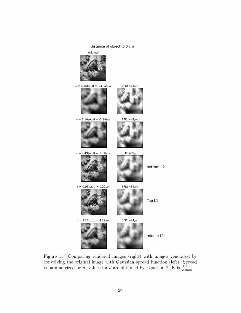
Figure 15: Comparing rendered images (right) with images generated byconvolving the original image with Gaussian spread function (left). Spreadis parametrized by σ; values for d are obtained by Equation 2. K is 117px

200µm.

20

case of the shifted receptor layers (bottom of L2 at BFD = 400µm) whichis not biologically accurate but results in a blur profile that is closer to theexpected one (see Figure 13 for shifted receptor layer images and left of Fig-ure15 for expected profile), it is still hard to judge where exactly the imageis sharpest. If the best image is not clearly distinguishable, and projectedimages are very similar over a range of sensor distances, information is lostand thus accurate determination of the object’s distance will be no longerpossible.Before concluding that the spider accomplishes the impossible task of esti-mating distances from images that do contain sufficient information, it makessense to consider what the spider actually sees. It is important to point outthat the images generated with our Blender model reflect the light whichwould fall onto un-occluded planes behind the lens. However, the receptorsin spider eyes are not 2D planes, but volumes. Accordingly, the thickness ofthe receptor layers may play a further role. It seems likely that photons canreact with the receptive segments of the photoreceptor over its whole length(i.e reactive segment is a long as the layer is thick), so that the “image” asreceived by the receptors may be rather an integration of all image planesthan the single images used in our dataset. Additionally, in order to reache.g the “bottom of L1” a photon must first pass all of L2 and the top parts ofthe receptive segments of L1 without being absorbed. So in order to modelaccurately how much light each receptor receives, it would be necessary tohave an idea on how likely photons are to be absorbed on different locationsof the retina.In this volume-scenario either the information on where exactly on the layerthe image is sharpest or how the defocus varies over the length of the layeris lost, unless there are some unknown intracellular mechanisms preserving it.

Future work From the performance of the algorithm and above consider-ations we can conclude that the model as based on Land’s findings [5] is tooabstract to be able to make conclusions about the spider’s DFD mechanism.The present understanding of the components of the jumping spider eye isstill incomplete, but further insights may be gained by including more of theknown details in the model.A possible next step would be to model the receptor spacing (Figure 4) moreaccurately. The particular spacing and layout of the receptors may in partcompensate for aberrations. An additional step may be to include more de-tails on the vertical arrangement of the receptors and to move from a staticmodel to a model which accounts for retina movements: According to Blest etal. [7] the receptor ends of both L2 and L1 form a stair-like structure, whichmight provide depth information when the eye performs scanning movements.

21

Also, in reality L1 and L2 are not parallel to each other but oriented in aangle. This arrangement could also provide additional depth informationwhen comparing inputs to the layers. These findings point to very differentmechanisms for determining distances than the ones used in CV DFD algo-rithms.Based on measurements in jumping spider species Plexippus Blest also sug-gest that the interface between the posterior chamber of the eye and thereceptors acts as a second lens. This would change the optical system andthus the way light falls onto the receptors, potentially resulting in betterdistinguishable depth-profiles.

Conclusions We present images created by a model of the AM eye ofspider species M. aeneolus and analyse why Subbarao’s DFD algorithm failsto estimate distance accurately on these images. We conclude that the modelas based on considerations and measurements by Land [5]is too abstact toallow inferences to be drawn about the spider’s DFD mechanism. We proposeanother straightforward way to quantify defocus and suggest further aspectsto be included into the model.

Acknowledgements

Many thanks to Charlotte Pachot for help with Zemax and ex-pertise in the domain of experimental and theoretical optics and toMichael Klemm for feedback on Blender and Luxrender aspects of theeye model. I would also like to thank Thijs Versloot, Isabelle Dicaireand Dario Izzo for helpful discussions.

References

[1] Murali Subbarao and Gopal Surya. Depth from defocus: a spatial do-main approach. International Journal of Computer Vision, 13(3):271–294, 1994.

[2] Murali Subbarao. Parallel depth recovery by changing camera parame-ters. In ICCV, pages 149–155, 1988.

[3] Subhasis Chaudhuri, AN Rajagopalan, and S Chaudhuri. Depth fromdefocus: a real aperture imaging approach, volume 3. Springer New York,1999.

[4] Takashi Nagata, Mitsumasa Koyanagi, Hisao Tsukamoto, Shinjiro Saeki,Kunio Isono, Yoshinori Shichida, Fumio Tokunaga, Michiyo Kinoshita,Kentaro Arikawa, and Akihisa Terakita. Depth perception from imagedefocus in a jumping spider. Science, 335(6067):469–471, 2012.

22

[5] MF Land. Structure of the retinae of the principal eyes of jumping spiders(salticidae: Dendryphantinae) in relation to visual optics. Journal ofexperimental biology, 51(2):443–470, 1969.

[6] Blender Online Community. Blender - a 3D modelling and renderingpackage. Blender Foundation, Blender Institute, Amsterdam, 2014.

[7] AD Blest, RC Hardie, P McIntyre, and DS Williams. The spectral sen-sitivities of identified receptors and the function of retinal tiering in theprincipal eyes of a jumping spider. Journal of Comparative Physiology,145(2):227–239, 1981.

23