bayesian analysis and computational methods for dynamic modeling
TRANSCRIPT

Bayesian Analysis and Computational Methods for
Dynamic Modeling
by
Jarad Bohart Niemi
Department of Statistical ScienceDuke University
Date:
Approved:
Mike West, Advisor
Jim Berger
Scott Schmidler
Carlos Carvalho
Dissertation submitted in partial fulfillment of the requirements for the degree ofDoctor of Philosophy in the Department of Statistical Science
in the Graduate School of Duke University2009

Abstract(Statistics)
Bayesian Analysis and Computational Methods for Dynamic
Modeling
by
Jarad Bohart Niemi
Department of Statistical ScienceDuke University
Date:
Approved:
Mike West, Advisor
Jim Berger
Scott Schmidler
Carlos Carvalho
An abstract of a dissertation submitted in partial fulfillment of the requirements forthe degree of Doctor of Philosophy in the Department of Statistical Science
in the Graduate School of Duke University2009

Copyright © 2009 by Jarad Bohart NiemiAll rights reserved except the rights granted by the
Creative Commons Attribution-Noncommercial Licence

Abstract
Dynamic models, also termed state-space models, comprise an extremely rich model
class for time series analysis. This dissertation focuses on building dynamic models
for a variety of contexts and computationally efficient methods for Bayesian inference
for simultaneous estimation of latent states and unknown fixed parameters.
Chapter 1 introduces dynamic models and methods of inference in these models
including standard approaches in Markov chain Monte Carlo and sequential Monte
Carlo methods.
Chapter 2 describes a novel method for jointly sampling the entire latent state vec-
tor in a nonlinear Gaussian dynamic model using a computationally efficient adaptive
mixture modeling procedure. This method, termed AM4, is embedded in an over-
all Markov chain Monte Carlo algorithm for estimating fixed parameters as well as
states.
In Chapter 3, AM4 is implemented in a few illustrative nonlinear models and
compared to standard existing methods. This chapter also looks at the effect of the
number of mixture components as well as length of the time series on the efficiency
of the method.
I then turn to biological applications in Chapter 4. I discuss modeling choices as
well as derivation of the dynamic model to be used in this application. Parameter
and state estimation are performed for both simulated and real data.
Chapter 5 extends the methodology introduced in Chapter 2 from nonlinear Gaus-
iv

sian models to general dynamic models. The method is then applied to a financial
stochastic volatility model on US $ - British £ exchange rates and identifies a limi-
tation in the current state-of-the-art method in that field.
Bayesian inference in the previous chapter is accomplished through Markov chain
Monte Carlo which is suitable for batch analyses, but computationally limiting in
sequential analysis. Chapter 6 introduces sequential Monte Carlo. It discusses two
methods currently available for simultaneous sequential estimation of latent states
and fixed parameters and then introduces a novel algorithm that reduces the key,
limiting degeneracy issue while being usable in a wide model class. This new method
is applied to a biological model discussed in Chapter 4.
Chapter 7 implements and compares novel sequential Monte Carlo algorithms in
the disease surveillance context modeling influenza epidemics.
Finally, Chapter 8 suggests areas for future work in both modeling and Bayesian
inference. Several appendices provide detailed technical support material as well as
relevant related work.
v

To Camille and Avalon
vi

Contents
Abstract iv
List of Tables xii
List of Figures xiv
List of Abbreviations and Symbols xviii
Acknowledgements xx
1 Introduction 1
2 Adaptive mixture modeling Metropolis method 5
2.1 Dynamic model and FFBS analysis . . . . . . . . . . . . . . . . . . . 7
2.2 Normal mixture model approximations . . . . . . . . . . . . . . . . . 8
2.2.1 Background and notation . . . . . . . . . . . . . . . . . . . . 8
2.2.2 Mixtures in dynamic models . . . . . . . . . . . . . . . . . . 9
2.2.3 Two-state example . . . . . . . . . . . . . . . . . . . . . . . . 11
2.2.4 Regenerating mixtures . . . . . . . . . . . . . . . . . . . . . . 11
2.3 Metropolis MCMC . . . . . . . . . . . . . . . . . . . . . . . . . . . . 15
2.3.1 Adaptive mixture model Metropolis for states . . . . . . . . . 15
2.3.2 Combined MCMC for states and fixed model parameters . . . 16
2.4 Summary . . . . . . . . . . . . . . . . . . . . . . . . . . . . . . . . . 17
3 Application to nonlinear Gaussian models 19
3.1 Dynamic linear model example . . . . . . . . . . . . . . . . . . . . . 21
vii

3.2 A trigonometric model . . . . . . . . . . . . . . . . . . . . . . . . . . 24
3.3 Illuminating example . . . . . . . . . . . . . . . . . . . . . . . . . . 26
3.3.1 Effect of the number of components . . . . . . . . . . . . . . . 31
3.3.2 Comparison to alternative MCMC schemes . . . . . . . . . . 31
3.4 Summary . . . . . . . . . . . . . . . . . . . . . . . . . . . . . . . . . 34
4 Parameter estimation in systems biology models 35
4.1 Synthetic biology . . . . . . . . . . . . . . . . . . . . . . . . . . . . . 36
4.2 Time-lapse fluorescent microscopy experiments . . . . . . . . . . . . 37
4.3 Modeling chemical reactions . . . . . . . . . . . . . . . . . . . . . . . 38
4.3.1 Biochemical system . . . . . . . . . . . . . . . . . . . . . . . 39
4.3.2 Deterministic chemical kinetics . . . . . . . . . . . . . . . . . 39
4.3.3 Stochastic chemical kinetics . . . . . . . . . . . . . . . . . . . 41
4.3.4 Chemical Langevin equation . . . . . . . . . . . . . . . . . . . 42
4.3.5 Dynamic nonlinear models . . . . . . . . . . . . . . . . . . . 43
4.4 Parameter estimation . . . . . . . . . . . . . . . . . . . . . . . . . . 44
4.5 Feedback of T7 RNA polymerase . . . . . . . . . . . . . . . . . . . . 47
4.5.1 Prior elicitation . . . . . . . . . . . . . . . . . . . . . . . . . 48
4.5.2 DnLM simulated data . . . . . . . . . . . . . . . . . . . . . . 50
4.5.3 Dynetica simulation . . . . . . . . . . . . . . . . . . . . . . . 53
4.5.4 Time-lapse fluorescent microscopy data . . . . . . . . . . . . . 58
4.6 Example motivated by pathway studies in systems biology . . . . . . 63
4.6.1 Multivariate states and parameters . . . . . . . . . . . . . . . 65
4.6.2 Mis-specified prior for nonlinear parameter . . . . . . . . . . . 70
4.6.3 Inference on unmeasured components . . . . . . . . . . . . . . 71
4.6.4 All fixed parameters and target level known . . . . . . . . . . 72
viii

4.6.5 Relaxing priors on fixed parameters . . . . . . . . . . . . . . 73
4.7 Summary . . . . . . . . . . . . . . . . . . . . . . . . . . . . . . . . . 77
5 Nonlinear, non-Gaussian models: an example in historical analysisof US dollar - British pound exchange Rate 79
5.1 Analysis of stochastic volatility models . . . . . . . . . . . . . . . . . 79
5.2 Non-Gaussian mixture updating . . . . . . . . . . . . . . . . . . . . 82
5.2.1 Updating filtered distributions in a stochastic volatility model 84
5.2.2 Metropolis-Hastings sampling of the volatility . . . . . . . . . 85
5.3 MCMC algorithm for stochastic volatility example . . . . . . . . . . . 86
5.4 Analysis of daily US $-British £ exchange rate time series . . . . . . 87
5.4.1 Informative prior for evolution variance . . . . . . . . . . . . . 88
5.4.2 Uninformative prior for evolution variance . . . . . . . . . . . 89
5.5 Summary . . . . . . . . . . . . . . . . . . . . . . . . . . . . . . . . . 92
6 Sequential Monte Carlo methods 94
6.1 Sequential Monte Carlo with known parameters . . . . . . . . . . . . 96
6.1.1 Importance sampling . . . . . . . . . . . . . . . . . . . . . . . 97
6.1.2 Sequential importance sampling . . . . . . . . . . . . . . . . . 98
6.1.3 Resampling . . . . . . . . . . . . . . . . . . . . . . . . . . . . 99
6.2 Sequential fixed parameter estimation . . . . . . . . . . . . . . . . . 100
6.2.1 Kernel smoothing . . . . . . . . . . . . . . . . . . . . . . . . 101
6.2.2 Parameter learning . . . . . . . . . . . . . . . . . . . . . . . . 101
6.2.3 Comparison of kernel smoothing with particle learning . . . . 104
6.3 Partial conditional sufficient structure . . . . . . . . . . . . . . . . . 109
6.4 Example motivated by pathway studies in systems biology . . . . . . 110
6.5 Summary . . . . . . . . . . . . . . . . . . . . . . . . . . . . . . . . . 112
ix

7 Sequential Monte Carlo methods for influenza outbreak detectionusing Google flu activity Estimate 115
7.1 Google flu activity estimate . . . . . . . . . . . . . . . . . . . . . . . 117
7.2 A model for influenza epidemic detection . . . . . . . . . . . . . . . 119
7.3 Sequential Monte Carlo methods for influenza detection . . . . . . . . 120
7.3.1 Particle learning for influenza detection . . . . . . . . . . . . 120
7.3.2 Kernel smoothing for influenza detection . . . . . . . . . . . . 123
7.3.3 Kernel smoothing with particle learning applied to influenzadata . . . . . . . . . . . . . . . . . . . . . . . . . . . . . . . . 125
7.4 Analysis of Google flutrend data . . . . . . . . . . . . . . . . . . . . . 125
7.5 Summary . . . . . . . . . . . . . . . . . . . . . . . . . . . . . . . . . 128
8 Additional discussion and future research 130
8.1 Adaptive mixture modeling . . . . . . . . . . . . . . . . . . . . . . . 130
8.2 Sequential Monte Carlo for fixed parameters . . . . . . . . . . . . . . 132
8.3 Systems and synthetic biology . . . . . . . . . . . . . . . . . . . . . . 134
8.4 Disease surveillance . . . . . . . . . . . . . . . . . . . . . . . . . . . . 136
A Differential equation model derivations 138
A.1 T7 RNA polymerase feedback . . . . . . . . . . . . . . . . . . . . . . 138
A.2 Tetramer feedback . . . . . . . . . . . . . . . . . . . . . . . . . . . . 140
B Updating a mixture of Gaussians prior using an arbitrary observa-tion model 141
B.1 Updating a single Gaussian . . . . . . . . . . . . . . . . . . . . . . . 141
B.2 Updating a mixture of Gaussians . . . . . . . . . . . . . . . . . . . . 143
C MCMC implementation details 145
C.1 Feedback of T7 RNA polymerase analysis . . . . . . . . . . . . . . . 145
C.2 Example motivated by pathway studies in systems biology . . . . . . 148
x
C.3 Analysis of US $-British £ exchange rate . . . . . . . . . . . . . . . 151
C.4 Comparison of kernel smoothing with particle learning . . . . . . . . 152
D MATLAB code for algorithm implementation 154
D.1 Mixture regeneration . . . . . . . . . . . . . . . . . . . . . . . . . . . 155
D.2 Adaptive mixture filtering . . . . . . . . . . . . . . . . . . . . . . . . 157
D.3 Backward sampling from an adaptive mixture filter . . . . . . . . . . 159
D.4 Metropolis acceptance probability component calculation . . . . . . . 160
D.5 Approximate updating of mixture components . . . . . . . . . . . . 162
D.6 AM4 for stochastic volatility model . . . . . . . . . . . . . . . . . . . 164
E Image segmentation and dynamic lineage analysis in single-cell flu-orescence microscopy 166
F A synthetic biology challenge: making cells compute 186
Bibliography 211
Biography 222
xi

List of Tables
2.1 Regenerating procedure . . . . . . . . . . . . . . . . . . . . . . . . . . 13
3.1 Empirical mean (sd) % acceptance rates from 100 simulations of the modeldefined by: ft(x) = x, gt(x) = sin(x), Vt = 1, Wt = 1 and x0 ∼ N(0, 10). . 25
3.2 Relative empirical mean (sd) computation time in minutes for 10,000iterations using the model in 3.1 . . . . . . . . . . . . . . . . . . . . . 26
4.1 Adaptive mixture filtering algorithm with sub-intervals . . . . . . . . 46
4.2 Backward sampling from adaptive mixture filter . . . . . . . . . . . . 47
5.1 Approximation to the distribution of a log(χ21)/2 random variable. . . 81
5.2 Equations for approximately updating a normal mixture given datafrom an arbitrary observation density. . . . . . . . . . . . . . . . . . . 83
5.3 Equations for approximately updating a normal mixture given datafrom a log(χ2
1)/2 observation density. . . . . . . . . . . . . . . . . . . 84
5.4 Algorithm for adaptive mixture filtering in the stochastic volatility modelshown in equations 5.1. . . . . . . . . . . . . . . . . . . . . . . . . . . 86
6.1 Kernel smoothing algorithm as described in Liu and West (2001) . . . 102
6.2 Particle learning algorithm as described in Carvalho et al. (2008) . . . 104
6.3 Sequential Monte Carlo algorithm combining kernel smoothing andparticle learning in models with partial sufficient statistics . . . . . . 110
7.1 Particle learning algorithm for analysis of the model of Section 7.2 . . 123
7.2 Kernel smoothing algorithm for analysis of the model of Section 7.2 . 124
xii

7.3 Algorithm combining kernel smoothing with particle learning for anal-ysis of the model of Section 7.2. The algorithm assumes a particleapproximation to p(θ−ρ, ρ, st−1, xt−1, zt−1|y1:(t−1)) is available at timet− 1, namely (θ−ρ, ρ, st−1, xt−1, zt−1)
(j), j ∈ 1, 2, . . . , J. . . . . . . . 126
A.1 Reactions describing the T7 RNA polymerase feedback system. . . . . 139
A.2 Differential equations for T7 RNA polymerase feedback system. . . . 139
A.3 Reactions describing an activator-target protein tetramer feedbacksystem. . . . . . . . . . . . . . . . . . . . . . . . . . . . . . . . . . . . 140
xiii

List of Figures
2.1 Gaussian mixture approximation of a bivariate distribution in a non-linear Gaussian model . . . . . . . . . . . . . . . . . . . . . . . . . . 12
2.2 Adaptive mixture filtering with no regeneration . . . . . . . . . . . . 14
2.3 Adaptive mixture filtering with regeneration . . . . . . . . . . . . . . 14
3.1 A realization y1:100 from a 1, 1, 1, 0.012 DLM with x0 ∼ N(0, 1). . . . . . 22
3.2 Traceplots of a randomly chosen state for the CPS (green), MRW (blue),and FFBS exact sampling (red). . . . . . . . . . . . . . . . . . . . . . . 23
3.3 Pointwise 95% credible intervals for the entire 101-dimensional state vectorfor the truth (black), FFBS exact sampling (red), CPS (green), and MRW(blue). . . . . . . . . . . . . . . . . . . . . . . . . . . . . . . . . . . . 23
3.4 Kernel density estimates based on 10,000 iterations of the MCMC for thesame state shown in Figure 3.2 for the truth (black), FFBS exact sampling(red), CPS (green), and MRW (blue). . . . . . . . . . . . . . . . . . . . 24
3.5 Simulated latent states (top) and observations (bottom) from the modelshown in equations 3.2. . . . . . . . . . . . . . . . . . . . . . . . . . . . 27
3.6 Adaptive mixture filtering densities using data from Figure 3.5 for selectedtime points that display markedly non-Gaussian behavior. . . . . . . . . . 28
3.7 Model of (3.2): Histograms of the smoothed samples for the same timepoints shown in 3.6. . . . . . . . . . . . . . . . . . . . . . . . . . . . . 28
3.8 Model of (3.2): Histograms of the smoothed samples for all time pointsshown vertically where brighter yellow indicates higher posterior mass. Thetrue states are shown as “*.” . . . . . . . . . . . . . . . . . . . . . . . 29
3.9 Model of (3.2): Scatterplot of MCMC samples for x71:72. . . . . . . . . . 30
3.10 Model of (3.2): Reconstruction of bivariate density p(x71,72|y1:100). . . . . 30
xiv

3.11 Traceplots for state x72 using 500, 1000, and 2000 components in themixture filtering procedure from the top to the bottom respectively. . 32
3.12 Traceplots for state x72 using CPS (green), MRW (blue), and AM4(red) MCMC methods under approximately the same computationaltime. . . . . . . . . . . . . . . . . . . . . . . . . . . . . . . . . . . . . 33
4.1 Time-lapse fluorescent microscopy data simulated from a DnLM . . . 51
4.2 Posterior plots for model parameters based on simulated data from aDnLM model . . . . . . . . . . . . . . . . . . . . . . . . . . . . . . . 52
4.3 Scatter plots for posterior draws of α versus d for low (red) and high (blue)production using DnLM simulated data. Truth shown as black Xs. . . . . 53
4.4 Posterior 95% credible intervals (blue) for the latent state series with thetruth (red) for DnLM simulated data. . . . . . . . . . . . . . . . . . . . 54
4.5 Dynetica schematic of T7 RNAP feedback . . . . . . . . . . . . . . . 55
4.6 Dynetica simulated time-lapse fluorescent microscopy data . . . . . . 56
4.7 Posterior plots for model parameters based on Dynetica simulated data 57
4.8 Scatter plots for posterior draws of α versus d for low (red) and high (blue)production using Dynetica simulated data. . . . . . . . . . . . . . . . . 58
4.9 Posterior 95% credible intervals (blue) for the latent state series with thetruth (red) for Dynetica simulated data. . . . . . . . . . . . . . . . . . . 59
4.10 Frames from a time-lapse fluorescent microscopy movie . . . . . . . . 60
4.11 Mean cellular fluorescence in two cells obtained using time-lapse fluorescentmicroscopy on 10-minute intervals. . . . . . . . . . . . . . . . . . . . . . 61
4.12 Posterior plots for model parameters based on real data . . . . . . . . 62
4.13 Scatter plots for posterior draws of α versus d for both cells using real data. 63
4.14 Posterior pointwise 95% credible intervals (blue) for the latent state seriesfor the real data. . . . . . . . . . . . . . . . . . . . . . . . . . . . . . . 64
4.15 Model of (4.6): Production and decay functions for various levels of theactivator. . . . . . . . . . . . . . . . . . . . . . . . . . . . . . . . . . 66
4.16 Model of (4.6): The upper plot shows the known level of activator and thelower plot shows the observation at all time points. . . . . . . . . . . . . 66
xv

4.17 Model of (4.6): Pointwise median (solid, blue) and 95% credible interval(dotted, blue) results for the target protein (black). The activator (red) isshown for reference. . . . . . . . . . . . . . . . . . . . . . . . . . . . . 67
4.18 Model of (4.7): Histograms of marginal posterior estimates (blue), prior(green), and true value (red) for fixed model parameters. . . . . . . . . . 69
4.19 Model of (4.7): Pointwise median (solid) and 95% credible interval (black)results for the underlying state (red) for the activator (top) and target(bottom) proteins. . . . . . . . . . . . . . . . . . . . . . . . . . . . . . 70
4.20 Model of (4.7): Histograms of marginal posterior estimates, prior, andtrue value for fixed model parameters when the prior for β is inaccurate. 71
4.21 Pointwise 95% credible intervals (dashed) and median (solid) for the prior(gray) and the posterior (black) for latent activator protein level when nomeasurements are taken on this protein and all fixed parameters are known. 73
4.22 Pointwise 95% credible intervals (dashed) and median (solid) for the prior(gray) and the posterior (black) for latent activator protein level when nomeasurements are taken on this protein and when the evolution variance isunknown. . . . . . . . . . . . . . . . . . . . . . . . . . . . . . . . . . . 74
4.23 Posterior histogram and prior (green) for the evolution standard deviationof the activator. . . . . . . . . . . . . . . . . . . . . . . . . . . . . . . 75
4.24 Pointwise 95% credible intervals (dashed) and median (solid) for the prior(gray) and the posterior (black) for latent activator protein level when nomeasurements are taken on this protein and all evolution parameters areunknown. . . . . . . . . . . . . . . . . . . . . . . . . . . . . . . . . . . 75
4.25 Posterior histogram and prior (green) for activator evolution parameters.Clockwise from top left the parameters are µ0, µ1, φ, and σa. . . . . . . . 76
5.1 Density of a log(χ21)/2 random variable (green) and a 7-component
mixture of Gaussians approximation (blue) with the 7 components(red). Left plot shows the left tail while the right plot shows the mainmass of the distribution. . . . . . . . . . . . . . . . . . . . . . . . . . 82
5.2 Prior (left) and posterior (right) for x under a randomly chosen priorand the observation model y = x+ ν where ν ∼ log(χ2
1)/2. . . . . . . 85
5.3 Changes in the daily spot exchange rate of the US dollar to the Britishpound over a period of 1000 days ending on 8/9/96. . . . . . . . . . . 88
xvi

5.4 Posterior histograms and priors (green) for stochastic volatility modelparameters using AM4 (blue) and KSC (red) when the evolution stan-dard deviation is given an informative prior. . . . . . . . . . . . . . 90
5.5 Pointwise 95% credible intervals for the volatility (σt) using AM4(blue) and KSC (red) where
√W is given an informative prior. . . . . 90
5.6 Posterior histograms and priors (green) for stochastic volatility modelparameters using AM4 (blue) and KSC (red) when the evolution stan-dard deviation is given a relatively uninformative prior. . . . . . . . . 91
5.7 Pointwise 95% credible intervals for the volatility (σt) using AM4(blue) and KSC (red) where
√W is given a relatively uninformative
prior. . . . . . . . . . . . . . . . . . . . . . . . . . . . . . . . . . . . . 91
6.1 Simulation from an autoregressive process observed with error. . . . . 105
6.2 Sequential filtered estimates of the median and 95% credible inter-vals for fixed model parameters as well as the latent state comparingMCMC and SMC using 1,000 particles in the SMC methods. . . . . . 107
6.3 Sequential filtered estimates of the median and 95% credible inter-vals for fixed model parameters as well as the latent state comparingMCMC and SMC using 10,000 particles in the SMC methods. . . . . 108
6.4 Model of (4.7): Histograms of marginal posterior estimates (blue), prior(green), and true value (red) for fixed model parameters based on an SMCanalysis. . . . . . . . . . . . . . . . . . . . . . . . . . . . . . . . . . . 113
6.5 Reproduction of Figure 4.18 . . . . . . . . . . . . . . . . . . . . . . . 113
7.1 Weekly reported Google flu activity estimate for North Carolina in-fluenza season (top) and first order differences (bottom) from mid-2004until mid-2008. . . . . . . . . . . . . . . . . . . . . . . . . . . . . . . 118
7.2 Sequential pointwise 95% credible intervals and means for fixed pa-rameters using the kernel smoothing (blue), particle learning (green),and kernel smoothing with particle learning (red) approaches on NorthCarolina Google flu activity estimate. . . . . . . . . . . . . . . . . . . 127
7.3 Sequential estimates of current epidemic probability based on kernelsmoothing (blue), particle learning (green), and kernel smoothing withparticle learning (red) approaches with scaled North Carolina Googleflu activity estimate (gray). . . . . . . . . . . . . . . . . . . . . . . . 129
xvii

List of Abbreviations and Symbols
Symbols
yt indicates the observation vector at time t.
xt indicates an unobserved latent state vector at time t.
θ indicates the fixed parameter vector.
ys:t indicates sequence of vectors ys, ys+1, . . . , yt where s < t.
y−j indicates either the vector y1:T or the vector y0:T with the jth
element removed where the choice should be clear from the con-text.
N(µ, σ2) indicates a normal distribution with mean µ and standard devi-ation σ.
N(x|µ, σ2) indicates the probability density function of a normal distribu-tion with mean µ and standard deviation σ evaluated at x.
N(x|µ, σ2)I(a < x < b) indicates the probability density function of a normal distri-bution with location parameter µ and scale parameter σ2. In thetext, this distribution is often referred to in terms of its expectedvalue (given below) and its “standard deviation” σ.
E[x] = µ+φ
(a−µσ
)− φ
(b−µσ
)Φ
(b−µσ
)− Φ
(a−µσ
)σwhere φ(·) is the probability density function and Φ(·) is thecumulative density function of the standard normal distribution.This distribution will also be referred to as a positive normal orpositive Gaussian distribution when a = 0 and b→∞.
Nm(p1:J ,m1:J , C1:J) indicates a discrete mixture of Gaussians with distribution
J∑j=1
pjN(mj, Cj).
xviii

χ2ν indicates a χ-squared random variable with ν degrees of freedom.
Ga(α, β) indicates a gamma distribution with shape parameter α and rateparameter β having mean α/β.
p(θ| . . .) indicates the full conditional distribution for θ, i.e. the proba-bility density function for θ given all other unknowns and thedata.
Abbreviations
AMM Adaptive mixture modeling; see Chapter 2.
AM4 Adaptive mixture modeling Metropolis method; see Chapter 2.
APF Auxiliary particle filter; see Pitt and Shephard (1999).
DLM Dynamic linear model, i.e. linear Gaussian model, defined bythe multiple Ft, Gt, Vt,Wt (see West and Harrison, 1997).
DnLM Dynamic nonlinear model, i.e. nonlinear Gaussian model.
FFBS Forward filtering backward sampling algorithm (see Carter andKohn, 1994; Fruhwirth-Schnatter, 1994).
MCMC Markov chain Monte Carlo
SMC Sequential Monte Carlo
SSM State space model
RNAP Ribonucleic acid (RNA) polymerase
xix

Acknowledgements
I would like to thank all those in the Department of Statistical Science for their
fantastic discussions about all things in life. In particular, I would like to thank
my advisor Mike West for his patience, support, and encouragement throughout my
time at Duke. I would also like to thank Carlos Carvalho for being a friend and a
mentor. Thanks goes to Lingchong You and Cheemeng Tan for many discussions
about biology and their drive to make bacteria work for us.
I also want to thank a number of colleagues for making my time here memorable.
Thank you to Eric Vance for making sure I arrived at Duke basketball games on
time, James Scott and Richard Hahn for competition on the squash court, Liang
Zang and Zhi Ouyang for enlightening discussions about Chinese culture, Joe Lucas
for great discussions after swim team practice, Jeff Sipe for letting me ride his horses,
Dan Merl for catching me when I fall, and Brian Reich for all things Minnesotan.
Thanks goes to my wife Camille who moved to NC without a ring on her finger.
Thank you for being my beautiful bride and bearing our wonderful daughter Avalon.
I believe she would also like to thank Michelle, Jill, Melanie, and Kristian for their
female companionship.
Finally, I would like to thank my family. My sister Libby for her free spirit. My
parents Bonnie and Jerry for their unconditional love and the solid foundation they
provided for me.
xx

1
Introduction
Technological advancements have dramatically increased our ability to gather and
store large amounts of data. Often these data are collected on a time scale, such
as minutes, days or weeks, and naturally lend themselves to time series analysis.
Examples include measurements of protein concentrations within bacterial cells, daily
monetary exchange rates, or weekly hospital visits for a particular disease. In each
of these cases, interest centers on the current and historical process driving the
observations, but also in the features controlling this process.
Dynamic models provide a natural tool for analyzing time series data of this sort
(West and Harrison, 1997; Harvey et al., 2004). This general class of discrete time
models is defined by an unobserved latent state that evolves through time and noisy
observations of that state. Inference is often accomplished using Bayesian methods
including Markov chain Monte Carlo (MCMC) and sequential Monte Carlo (SMC)
methodologies. MCMC naturally lends itself to batch analysis of historical data
whereas SMC is more appropriate for online analysis and decisions. This thesis fo-
cuses on incorporating mixtures of distributions to improve computational efficiency
of both MCMC and SMC methods of inference in dynamic models.
1

MCMC analysis in dynamic models is often accomplished by decomposing the
sampling scheme into iteratively sampling the states conditional on the fixed pa-
rameters and then sampling the fixed parameters conditional on the states. This
uses a combination of Gibbs (Geman and Geman, 1984) and Metropolis-Hastings
(Metropolis et al., 1953; Hastings, 1970) steps (Gelfand and Smith, 1990). In the
particular case of linear Gaussian models, states can be sampled jointly using a
a special Gibbs sampling step called forward filtering backward sampling (FFBS)
(Fruhwirth-Schnatter, 1994; Carter and Kohn, 1994) which incorporates use of the
well-known Kalman filter (Kalman, 1960). Fixed parameters, such as autoregres-
sive parameters and variances, can then be sampled using Gibbs steps common to
multivariate regression.
For nonlinear Gaussian models, sampling states, parameters, or both may not be
available as Gibbs steps. In Chapter 2, I introduce the adaptive mixture modeling
Metropolis method (AM4) to sample jointly from the set of states. This methodol-
ogy utilizes ideas of approximating filtering densities using mixtures of many precise
Gaussian components to accurately capture nonlinearities in the model (Harrison
and Stevens, 1971; Sorenson and Alspach, 1971; Alspach and Sorenson, 1972). Back-
ward sampling from these mixtures provides a proposed sample for the states which
is then accepted according to a Metropolis acceptance probability. Advantages of
this method over standard approaches are discussed in Chapter 3 using a variety of
simulated examples.
Nonlinear Gaussian models arise in application in systems biology (Wilkinson,
2006). Chapter 4 discusses a primary motivating example of building statistical
models to represent the dynamics of protein concentrations within individual cells.
These dynamics are responsible for cellular functions including proliferation, com-
munication, and apoptosis as well as in unregulated cell growth leading to cancer.
Statistical models representing these dynamics are useful in understanding and sug-
2
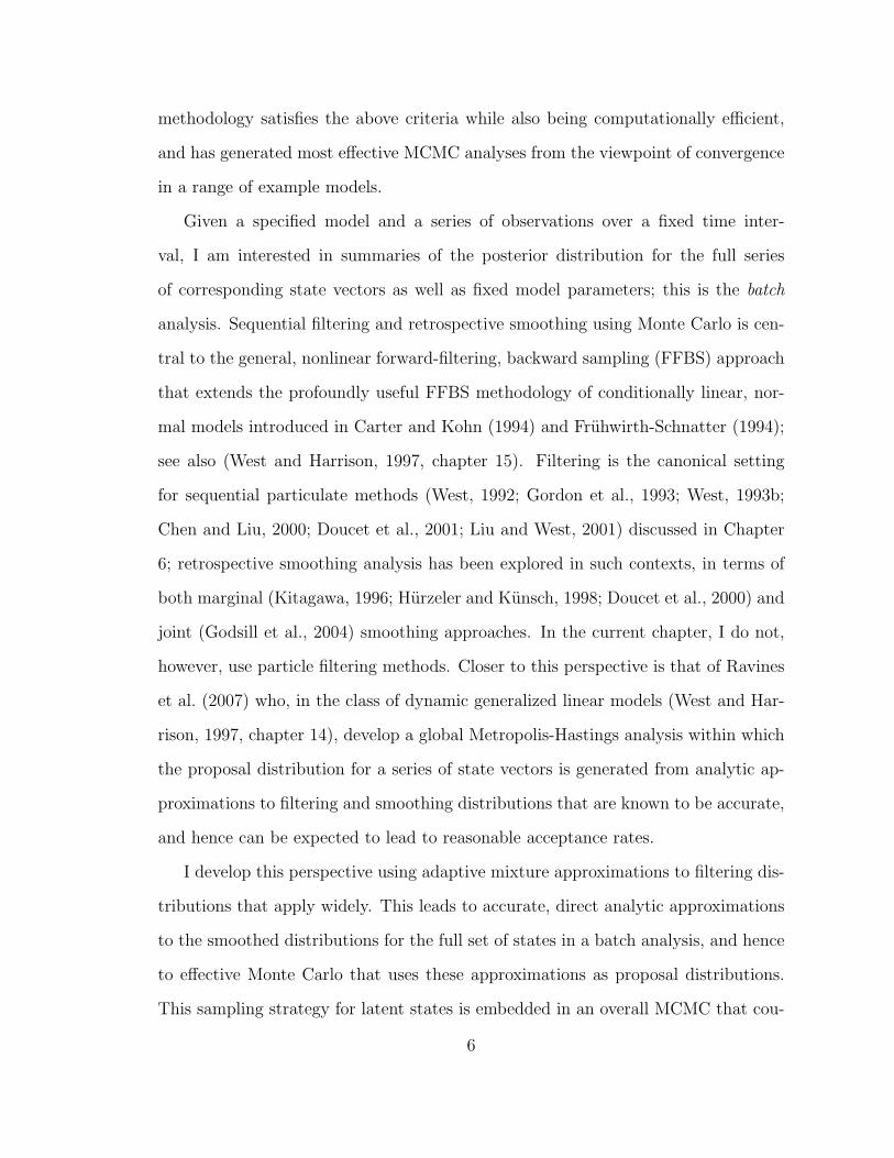
gesting therapeutic interventions to fight cancer progression. I use the AM4 method-
ology to analyze protein dynamics in both real and simulated data where inferences
on latent states as well as fixed model parameters are of primary importance.
Chapter 5 extends the AM4 methodology to more general dynamic models. The
similarity with nonlinear Gaussian models is that the filtered distribution for the
states is still approximated by a mixture of Gaussians, but mixture components can
no longer be updated based on a Taylor series expansion of the nonlinear function.
Instead, the whole distribution itself is approximated allowing for approximate mix-
ture component updating as described in Appendix B. I apply this technique to a
stochastic volatility model based on monetary exchange rate data.
In Chapter 6, I discuss online analysis using SMC methods often referred to as
particle filters. When all fixed parameters are known, a widely used strategy for
Monte Carlo filtering of states is known as the bootstrap filter which implements se-
quential importance sampling with resampling (Gordon et al., 1993). Unfortunately
for unknown fixed parameters, this approach is ineffective as the number of Monte
Carlo samples representing the fixed parameters rapidly reduces to one. This de-
generacy is counteracted by methodologies that allow for new samples to be drawn
throughout the procedure using kernel smoothing (West, 1993b; Liu and West, 2001)
or sufficient statistic (Fearnhead, 2002; Carvalho et al., 2008) ideas. I combine these
ideas to produce an efficient yet widely applicable method for simultaneous sequential
estimation of both parameters and states.
A motivating example for this context concerns influenza activity data for rapid
alerting of impending epidemics. Previous research in this area has utilized MCMC
methods sequentially for data analysis (Martınez-Beneito et al., 2008). As the reso-
lution of the data increases and the length of time increases, these methods quickly
become computationally infeasible. In Chapter 7, I build a dynamic model and im-
plement novel SMC methods to analyze Google flu activity estimates for influenza
3

surveillance.
This thesis builds dynamic models for a variety of applications and describes al-
gorithms for MCMC and SMC inference in these models that increase computational
efficiency. There are many possible extensions and areas for future work which are
discussed in Chapter 8.
4

2
Adaptive mixture modeling Metropolis method
Motivated by problems of fitting and assessing structured, nonlinear dynamic mod-
els to time series data arising in studies of cellular networks in systems biology, I
revisit the problem of Bayesian inference on latent, time-evolving states and fixed
model parameters in a dynamic model context. In recent years, this general area
has seen development of a number of customized Monte Carlo methods, but ex-
isting approaches do not yet provide the kind of comprehensive, robust, generally
and automatically applicable computational methods needed for repeat batch anal-
ysis in routine application. The above criteria for effective statistical computation
are central to my primary motivating context of dynamic cellular networks, an ap-
plied field that is beginning to grow rapidly as relevant high-resolution time series
data on genetic circuitry becomes increasing available in single-cell and related stud-
ies (Rosenfeld et al., 2005; Golightly and Wilkinson, 2005; Wilkinson, 2006; Wang
et al., 2009) and synthetic bioengineering (Tan et al., 2007). With this motivation,
I build on the best available analytic and Monte Carlo tools for nonlinear dynamic
models to generate a novel adaptive mixture modeling Metropolis method (AM4) that
is embedded in an overall MCMC strategy for posterior computation; the resulting
5
methodology satisfies the above criteria while also being computationally efficient,
and has generated most effective MCMC analyses from the viewpoint of convergence
in a range of example models.
Given a specified model and a series of observations over a fixed time inter-
val, I am interested in summaries of the posterior distribution for the full series
of corresponding state vectors as well as fixed model parameters; this is the batch
analysis. Sequential filtering and retrospective smoothing using Monte Carlo is cen-
tral to the general, nonlinear forward-filtering, backward sampling (FFBS) approach
that extends the profoundly useful FFBS methodology of conditionally linear, nor-
mal models introduced in Carter and Kohn (1994) and Fruhwirth-Schnatter (1994);
see also (West and Harrison, 1997, chapter 15). Filtering is the canonical setting
for sequential particulate methods (West, 1992; Gordon et al., 1993; West, 1993b;
Chen and Liu, 2000; Doucet et al., 2001; Liu and West, 2001) discussed in Chapter
6; retrospective smoothing analysis has been explored in such contexts, in terms of
both marginal (Kitagawa, 1996; Hurzeler and Kunsch, 1998; Doucet et al., 2000) and
joint (Godsill et al., 2004) smoothing approaches. In the current chapter, I do not,
however, use particle filtering methods. Closer to this perspective is that of Ravines
et al. (2007) who, in the class of dynamic generalized linear models (West and Har-
rison, 1997, chapter 14), develop a global Metropolis-Hastings analysis within which
the proposal distribution for a series of state vectors is generated from analytic ap-
proximations to filtering and smoothing distributions that are known to be accurate,
and hence can be expected to lead to reasonable acceptance rates.
I develop this perspective using adaptive mixture approximations to filtering dis-
tributions that apply widely. This leads to accurate, direct analytic approximations
to the smoothed distributions for the full set of states in a batch analysis, and hence
to effective Monte Carlo that uses these approximations as proposal distributions.
This sampling strategy for latent states is embedded in an overall MCMC that cou-
6

ples in samplers for fixed model parameters to define a complete analysis.
2.1 Dynamic model and FFBS analysis
Begin with the Markovian dynamic model (West and Harrison, 1997)
yt =ft(xt) + νt (observation equation) (2.1a)
xt =gt(xt−1) + ωt (state evolution equation) (2.1b)
where xt is the unobserved state of the system at time t, yt is the observation at
time t, ft(·) and gt(·) are known, nonlinear observation and evolution functions, and
νt ∼ N(0, Vt) and ωt ∼ N(0,Wt) are independent and mutually independent Gaus-
sian innovations, the observation and evolution noise terms, respectively. Initially,
assume any model parameters in the nonlinear functions or noise variances are known
although those assumptions are relaxed in Chapters 4 and 5. Note that the develop-
ment can be extended well beyond the focus here on additive, normal noise terms,
though for specificity I focus on that structure here. Chapter 5 discusses dealing
with non-additive, non-Gaussian terms.
Based on the batch of data y1:T , the main goal is simulation of the set of states
x0:T from the implied posterior
p(x0:T |y1:T ) ∝ p(x0)T∏t=1
p(yt|xt)p(xt|xt−1) (2.2)
where p(x0) is the density of the initial state and p(yt|xt) and p(xt|xt−1) are defined
by equations (2.1a) and (2.1b), respectively. This is done using the FFBS strategy:
• FF: For each t = 1 :T sequentially process the datum yt to update numerical
summaries of the filtering densities p(xt|y1:t) at time t.
• BS: Simulate the joint distribution in equation (2.2) via the implied backward
7

compositional form
p(x0:T |y1:T ) ∝ p(xT |y1:T )T∏t=1
p(xt−1|xt, y1:(t−1)). (2.3)
That is:
1. draw xT ∼ p(xT |y1:T ) and set t = T ;
2. draw xt−1 ∼ p(xt−1|xt, y1:(t−1));
3. reduce t to t− 1 and return to step 2; stop when t = 0.
This generates the full joint sample x0:T in reverse order. All steps of FFBS depend
fundamentally on the structure of the joint densities
p(yt, xt, xt−1|y1:(t−1)) = p(yt|xt)p(xt|xt−1)p(xt−1|y1:(t−1)). (2.4)
In particular, filtering relies on the ability to compute and summarize
p(xt|y1:t) ∝ p(yt|xt)∫p(xt|xt−1)p(xt−1|y1:(t−1))dxt−1 =
∫p(yt, xt, xt−1|y1:(t−1))dxt−1
(2.5)
while backward sampling relies on the ability to simulate from
p(xt−1|xt, y1:(t−1)) ∝ p(xt−1|y1:(t−1))p(xt|xt−1) = p(xt, xt−1|y1:(t−1)), (2.6)
the bivariate margin of equation (2.4). In linear, Gaussian dynamic models, these
distributions are all Gaussian; in nonlinear models, the implied computations can
only be done using some form of approximation.
2.2 Normal mixture model approximations
2.2.1 Background and notation
This strategy is based on approximation of the sequentially updated distributions of
states via mixtures of many, very precise normal components. Mixtures have been
8

used broadly in dynamic modeling, for both model specification and computational
methods, especially in adaptive multi-process models and to represent model uncer-
tainty in terms of multiple models analyzed in parallel (West and Harrison, 1997,
chapter 12 and references therein). The basic idea of normal mixture approximation
in nonlinear dynamic models in fact goes back several decades to at least Harrison
and Stevens (1971) in statistics and Sorenson and Alspach (1971) in engineering, the
latter using the term Gaussian sum for direct analytic approximations to nonlinear
models; see also Alspach and Sorenson (1972) and Harrison and Stevens (1976). The
method here is a direct extension of the original Gaussian sum approximation idea
now embedded in the Markov chain Monte Carlo framework. The approach builds
on the concept of using mixtures of many precise normal components to approxi-
mate sequences of posterior distributions for sets of states as the conditioning data
is updated; in essence, this revisits and revises earlier adaptive importance sampling
approaches (West, 1992, 1993a,b) to be based on far more efficient – computationally
and statistically – Metropolis accept/reject methods.
2.2.2 Mixtures in dynamic models
Suppose at time t− 1 the density p(xt−1|y1:(t−1)) is – either exactly or approximately
– given by
(xt−1|y1:(t−1)) ∼ Nm(pt−1,1:J ,mt−1,1:J , Ct−1,1:J)
whereNm(p1:J ,m1:J , C1:J) represents a J-component mixture of Gaussians with com-
ponent N(mj, Cj) having probability pj for j ∈ 1, 2, . . . , J. Then the key trivariate
density of equation (2.4) is
p(yt, xt, xt−1|y1:(t−1)) =J∑j=1
pt−1,jp(yt|xt)p(xt|xt−1)N(xt−1|mt−1,j, Ct−1,j). (2.7)
9

Suppose that component variances Ct−1,1:J are very small relative to the variances
Vt,Wt and inversely related to the local gradients of the regression and evolution
functions ft(·), gt(·) in equation (2.1); this generally requires a large value of J. Then
variation of component j of the summand in equation (2.7) is heavily restricted to
the implied, small region around xt−1 = mt−1,j and gt(·) and ft(·) can be accurately
approximated with local linearization valid in that small region. The two lead terms
in summand j are replaced by the local normal, linear forms (xt|xt−1) ∼ N(at,j +
g′t(mt−1,j)(xt−1−mt−1,j),Wt) with at,j = gt(mt−1,j) and (yt|xt) ∼ N(ft,j+f′t(at,j)(xt−
at,j), Vt) with ft,j = ft(at,j) where f ′t(·) and g′t(·) indicate the derivatives of the
observation and evolution functions, respectively. This immediately reduces equation
(2.7) to a mixture of trivariate normals, so that all marginals and conditionals are
computable as normal mixtures. In particular, the key distributions for filtering and
smoothing are:
The equation (2.5) for forward filtering:
(xt|y1:t) ∼ Nm(pt,1:J ,mt,1:J , Ct,1:J) (2.8)
having elements mt,j = at,j + At,j(yt − ft,j) and Ct,j = Rt,j − A2t,jQt,j where At,j =
Rt,jf′t(at,j)/Qt,j, Rt,j = Ct−1,j[g
′t(mt−1,j)]
2 + Wt and Qt,j = Rt,j[f′t(at,j)]
2 + Vt. The
component probabilities are updated via pt,j ∝ pt−1,jN(yt|ft,j, Qt,j). This adaptive
mixture modeling (AMM) procedure produces a sequence of Gaussian mixtures that
approximate the sequence of state filtering distributions. Code for this approximate
forward filtering is provided in Appendix D.2.
The equation (2.6) for backward sampling:
(xt−1|xt, y1:(t−1)) ∼ Nm(qt,1:J , ht,1:J , Ht,1:J) (2.9)
having elements ht,j = mt−1,j+Bt,j(xt−at,j) and Ht,j = Ct−1,j−B2t,jRt,j where Bt,j =
Ct−1,jg′t(mt−1,j)/Rt,j; the component probabilities are qt,j ∝ pt−1,jN(xt|at,j, Rt,j).
Code for backward sampling is available in Appendix D.3.
10

For large J and small enough Ct−1,j, the implied filtering computations will pro-
vide a good approximation to the true model analysis, and have been used quite
widely in applications in engineering and elsewhere for some years. Smoothing com-
putations based on the approximations are direct, but have been less widely used
and exploited to date. Our strategy is to embed these mixture computations in an
overall MCMC, using them to define a global Metropolis proposal distribution for
p(x0:T |y1:T ). As a nice by-product, the observed Metropolis acceptance rates also
provide an indirect assessment of the adequacy of the Gaussian method as a direct
analytic approximation, though our interest is its use in obtaining exact posterior
samples.
2.2.3 Two-state example
To clearly fix ideas, Figure 2.1 shows aspects of an example with gt(x) = 0.1x3 +
sin(5x), Wt = 0.2 and in which (xt−1|y1:(t−1)) is a J = 50 component mixture with
resulting density graphed in the figure. The comparison between the bivariate con-
tours of the exact and mixture approximation of p(xt, xt−1|y1:(t−1)) demonstrates the
efficacy of the method in this highly nonlinear model. Evidently, the mixture model
is an accurate representation of the true nonlinear model, though the joint mixture
density is in fact very slightly more diffuse – a good attribute from the viewpoint
of the goal of generating a useful Metropolis proposal distribution. Approximation
accuracy increases with the number of normal mixture components used so long as
the variances Ct−1,j fall off appropriately as J increases, as discussed further below.
2.2.4 Regenerating mixtures
The basic mixture approximation strategy can work well when the component means
are spread out, the component variances are small, and the component probabilities
are approximately equal. The spread of component means leads to desirable wide-
11

Figure 2.1: Bivariate and marginal distributions for two-states in a modelwith gt(x) = 0.1x3 + sin(5x) and Wt = 0.2, and where p(xt−1|y1:(t−1)) is aJ = 50 component mixture with density graphed on the horizontal axis ofeach frame. The left pane shows exact bivariate density contours and, on thevertical axis, the implied margin for (xt|y1:(t−1)). The right pane shows thecorresponding 50−component mixture approximations. In each frame, thedashed line shows the evolution function gt(·).
ranging evaluations of the nonlinear evolution and observation functions. Very small
component variances improve the validity of the local linear approximations to the
nonlinear functions over increasingly small regions. Balanced component probabili-
ties ensure that each component contributes to the mixture after propagation through
the nonlinearities; if only a few components dominate, it is as if all other components
are irrelevant and the overall strategy will collapse.
These properties are explicitly maintained using a novel regenerating procedure
shown in Table 2.1. Suppose we wish to approximate an arbitrary density p(x) using
an equally-weighted mixture of Gaussians with means set at the J-quantiles of p(x)
and component variances constant and chosen so that the variance of the mixture
equals that of p(x). For large J, this satisfies the above desiderata for mixture
12
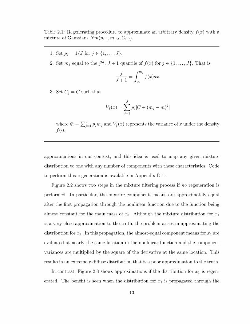
Table 2.1: Regenerating procedure to approximate an arbitrary density f(x) with amixture of Gaussians Nm(p1:J ,m1:J , C1:J).
1. Set pj = 1/J for j ∈ 1, . . . , J.
2. Set mj equal to the jth, J + 1 quantile of f(x) for j ∈ 1, . . . , J. That is
j
J + 1=
∫ mj
∞f(x)dx.
3. Set Cj = C such that
Vf (x) =J∑j=1
pj[C + (mj − m)2]
where m =∑J
j=1 pjmj and Vf (x) represents the variance of x under the density
f(·).
approximations in our context, and this idea is used to map any given mixture
distribution to one with any number of components with these characteristics. Code
to perform this regeneration is available in Appendix D.1.
Figure 2.2 shows two steps in the mixture filtering process if no regeneration is
performed. In particular, the mixture components means are approximately equal
after the first propagation through the nonlinear function due to the function being
almost constant for the main mass of x0. Although the mixture distribution for x1
is a very close approximation to the truth, the problem arises in approximating the
distribution for x2. In this propagation, the almost-equal component means for x1 are
evaluated at nearly the same location in the nonlinear function and the component
variances are multiplied by the square of the derivative at the same location. This
results in an extremely diffuse distribution that is a poor approximation to the truth.
In contrast, Figure 2.3 shows approximations if the distribution for x1 is regen-
erated. The benefit is seen when the distribution for x1 is propagated through the
13

Figure 2.2: Left pane shows the prior for x0 along the x-axis and the priorfor x1 on the right side of the y-axis after propagation through the nonlinearfunction (blue). Right pane shows the prior for x1 now on the x-axis with noregeneration and the prior for x2 on the left side of the y-axis while the truthis along the right side (magenta). The location of the mixture componentmeans for each prior are shown in green.
Figure 2.3: Left pane shows the prior for x0 along the x-axis and the priorfor x1 on the right side of the y-axis after propagation through the nonlinearfunction (blue). Right pane shows the prior for x1 now on the x-axis withregeneration and the prior for x2 on the left side of the y-axis while the truthis along the right side (magenta). The location of the mixture componentmeans for each prior are shown in green.
14

nonlinear function to approximate the distribution for x2. In this process, the mix-
ture component means for x2 are diffuse and provide a very good approximation to
the truth. This example is extreme, but it displays in two steps what I have seen
occur in practice in multiple steps of a non-regenerated mixture filter.
In the model of equation (2.1), suppose an initial prior p(x0) is defined as a
mixture, either directly or by applying the procedure of Table 2.1 to an original
prior and using a large value J. I proceed through the sequential updating analysis,
now where necessary using the regenerating procedure on the prior p(xt|xt−1, y1:(t−1))
and posterior p(xt|y1:t) to revise, balance and hence improve the overall adequacy of
the approximation at each stage.
2.3 Metropolis MCMC
2.3.1 Adaptive mixture model Metropolis for states
The mixture modeling strategy defines a computationally feasible method for eval-
uating and sampling from a useful approximation to the full joint posterior density
of states of equation (2.2) and, in reverse form, equation (2.3). Forward filtering
computations apply to sequentially update the mixture forms p(xt|y1:t) over t = 1:T
using equation (2.8) and the regenerating procedure of Table 2.1. This is followed
by backward sampling over t = T, T − 1, . . . , 0 using the mixture forms of equation
(2.9). Write q(x0:T |y1:T ) for the implied joint density of states from this analysis;
that is, q(·|y1:T ) has the form of the reverse equation (2.3) in which each p(·|·) is
replaced by the corresponding mixture density.
I treat the analysis via Metropolis-Hasting MCMC analysis. With a current
sample of states x0:T , apply the FFBS to generate a new, candidate draw x∗0:T from
the proposal distribution with density q(x0:T |y1:T ). This is assessed via the standard
15
accept/reject test, accepting x∗0:T with probability
ρ(x∗0:T , x0:T ) = min 1, w(x∗0:T )/w(x0:T ) (2.10)
where w(·) = p(·|y1:T )/q(·|y1:T ). Calculating p(·|y1:T ) is straight-forward given the
standard decomposition of state-space models shown in equation (2.2). Calculating
q(·|y1:T ) can be accomplished using the backward sampling decomposition shown in
equation (2.3). In addition, many of the required component probabilities, means,
and variances have been pre-calculated during the filtering and backward sampling
steps. Code to calculate p(·|y1:T ) and q(·|y1:T ) for a given draw is available in Ap-
pendix D.4.
This is a global MCMC, applying to the full set of consecutive states, that will gen-
erally define an ergodic Markov chain on x0:T based on everywhere-positivity of both
p(x0:T |y1:T ) and q(x0:T |y1:T ). As q is expected to provide a good global approxima-
tion, the resulting MCMC can be expected to perform well, and as mentioned above
the acceptance rates provide some indication of the accuracy of the approximation.
Evidently, acceptance rates can generally be expected to decay with increasing time
series length T. Experiences of Ravines et al. (2007) in the simpler DGLM context
and in my own experiments in this and related model contexts, bear out the utility
of the method. Additional comments and numerical comparisons of acceptance rates
appear in Chapter 3.
2.3.2 Combined MCMC for states and fixed model parameters
Practical applications involve models with fixed, uncertain parameters as well as the
latent states, and a complete analysis embeds the above simulator for states within
an overall MCMC that also includes parameters (e.g., see West and Harrison, 1997,
section 15.2). With a vector of parameters θ, extend the model notation to
yt = ft(xt|θ) + νt, xt = gt(xt−1|θ) + ωt,
16

where, now, the initial prior p(x0|θ) may involve elements of θ as may the variances
Vt,Wt (one key case being constant, unknown variances that are then elements of θ).
The overall computational strategy is then to apply the above state sampler at
each stage of an overall MCMC conditional on θ, and to couple this with resampling
of θ values using the implied distribution p(θ|x0:T , y1:T ) at each step of the chain.
Depending on the model form and priors specified for θ parameters, this will typically
be performed in terms of a series of Gibbs sampling steps, perhaps with some blocking
of subsets of parameters. Under a specified prior p(θ), the complete conditional
posterior for any subset of elements θi given the remaining elements θ−i is
p(θi|θ−i, x0:T , y1:T ) ∝ p(θ)p(x0|θ)T∏t=1
p(yt|xt, θ)p(xt|xt−1, θ). (2.11)
Sometimes this conditional can be sampled directly; a key example is when V =
Vt,W = Wt and θi = (V,W ) when, under independent inverse gamma priors, the
above conditional posterior is also the product of independent inverse gammas. In
other cases, resampling some elements θi will use random-walk Metropolis-Hastings
methods involving an accept/reject test to resample θi, i.e., a standard Metropolis-
within-Gibbs series of moves. So long as the prior density p(θ) that can be directly
and easily evaluated up to a constant, such moves are easy to implement since the
terms in equation (2.11) can be trivially evaluated at any point θ. Full MCMC
analyses with unknown fixed model parameters is explored in Chapter 4.
2.4 Summary
This chapter introduced methodology for jointly sampling a latent state vector in
a dynamic model using an independent Metropolis algorithm. The methodology
mimics the approach of FFBS where filtering is performed on states and samples
are obtained in reverse chronology. Filtering is accomplished using an adaptive
17

mixture filter based on a large number of mixture components to accurately capture
nonlinearities in the model. Regenerating these mixture components is required to
eliminate situations where one component dominates the mixture.
The goal of this methodology is to increase Markov chain mixing by eliminating
high autocorrelation between draws for states in successive iterations in an MCMC.
At the current time the method is univariate and therefore multivariate states are
sampled from iteratively as univariate state vectors conditional on the others. This
approach has been successfully used in the example models studied in Chapter 4.
Nonetheless models with a high degree of correlation between state vectors may,
for computational efficiency reasons, require block updating the multivariate state
vectors simultaneously.
The next chapter analyzes a number of examples to illustrate the improvement in
Markov chain mixing using this method relative to standard MCMC methodologies.
The following chapter builds dynamic models for biological application with unknown
fixed parameters analyzed using AM4 as part of an overall MCMC approach.
18

3
Application to nonlinear Gaussian models
This chapter studies several examples of nonlinear Gaussian models (West and Har-
rison, 1997, Ch. 13 ). This class of models is characterized by the model described
in equations (2.1) where either or both of the observation and evolution equation
means depend on a nonlinear function of the state and the errors for both equa-
tions are Gaussian. In this chapter, I am concerned with estimation of the state
in both the filtering and smoothing contexts while all fixed parameters are known.
The joint distribution for the entire latent state vector in these models is unavailable
analytically and therefore approximations are required for inference on those states.
The literature for this class of models and their analysis is large; I present a short
summary here.
In the deterministic filtering context, the most common approach is to use the
extended Kalman filter which simply linearizes both the observation and evolution
equations using a Taylor series expansion around the expected value of the state. Im-
provements to this approach use mixtures of Gaussians (Harrison and Stevens, 1971;
Sorenson and Alspach, 1971; Alspach and Sorenson, 1972; Ito and Xiong, 2000).
19

The use of mixtures allows for more flexibility and accuracy in modeling nonlineari-
ties. Alternative deterministic filters include the unscented Kalman filter (Julier and
Uhlmann, 1997) and Gauss-Hermite quadrature filtering (Arasaratnam et al., 2007),
but are not explored here.
Alternative Monte Carlo filtering strategies are based on sequential importance
sampling, often called particle filters. One of the early successful implementations is
in Gordon et al. (1993) who termed their algorithm the bootstrap filter. Improvements
on their methodology involve combinations of importance sampling, resampling, and
local MCMC moves (Kitagawa, 1996; Pitt and Shephard, 1999; Liu and Chen, 1998;
Doucet et al., 2000). Doucet et al. (2001) provides a good overview.
Inferential approaches to smoothing are important both for batch analyses of time
series data, but also in the context of a larger MCMC scheme involving unknown
fixed parameters. In these models, smoothing is often accomplished using Monte
Carlo strategies. In principle the deterministic filters could be used as proposals
for Metropolis algorithms and, perhaps, even for rejection or importance sampling.
Godsill et al. (2004) introduce a generic algorithm for smoothing in the particle
filtering framework. Other options, such as global approximation of the smoothed
state distribution, are possible (Jungbacker and Koopman, 2007).
In the following sections, I use the methodology developed in Chapter 2 to analyze
a number of models. Despite the title of this chapter, I initially look at a linear
Gaussian model to emphasize the importance of joint sampling of the latent states
in these models. I then move on to a trigonometric model to analyze the effect of
length of the time series and number of components on the Metropolis acceptance
rate. Finally, I end with an illuminating example of a highly nonlinear model which
produces a multi-modal posterior.
20

3.1 Dynamic linear model example
Dynamic linear models (DLMs) are defined by the observation and evolution equa-
tions
yt =F ′txt + νt (3.1a)
xt =Gtxt−1 + ωt (3.1b)
where Ft and Gt are known matrices and νt ∼ N(0, Vt) and ωt ∼ N(0,Wt) are
independent across time and mutually independent. This DLM is defined by the
quadruple Ft, Gt, Vt,Wt for each t, which along with p(x0), complete specification of
the Bayesian model. Of current interest is the distribution for the latent state vector
x0:T conditional on the observed data y1:T . In contrast to the analytically intractable
latent state distribution found in nonlinear Gaussian models, this distribution in
DLMs is available in closed form. This is true regardless of whether we are interested
in the prior, smoothed, marginal, or conditional distributions for this state vector.
For illustrative purposes, I compare three alternative MCMC sampling schemes
for obtaining samples from the smoothed state distribution p(x0:T |y1:T ):
1. one state at a time (Carlin et al., 1992) which I will refer to as CPS,
2. a multivariate random walk referred to as MRW, and
3. FFBS (Fruhwirth-Schnatter, 1994; Carter and Kohn, 1994).
The CPS approach uses Gibbs sampling to draw from the full conditional distribution
of each state conditional on all other states. Due to the conditional independence
structure in the model, p(xt|x−t, y1:T ) = p(xt|xt−1, xt+1, yt) for t ∈ 1, 2, . . . , T −
1 and similar results for the two end points x0 and xT . The simplification of
these full conditionals makes the CPS approach attractive. The MRW proposes
a value x∗0:T ∼ N(x0:T , σ2I) where I is the identity matrix with dimension T+1. The
21

Figure 3.1: A realization y1:100 from a 1, 1, 1, 0.012 DLM with x0 ∼N(0, 1).
Metropolis acceptance probability is ρ(x∗0:T , x0:T ) = min1, p(x∗0:T |y1:T )/p(x0:T |y1:T )
where p(x0:T |y1:T ) is calculated using equation (2.2). FFBS, the final scheme, in
DLMs is equivalent to the method described in Chapter 2 when J = 1. It provides
exact draws from the desired posterior. The computational time for these three
schemes is approximately equal and therefore each was run for 10,000 iterations
starting from the same initial point sampled from the true posterior.
The model used to compare these MCMC sampling schemes is shown in equations
(3.1) with Ft = Gt = Vt = 1, and Wt = 0.012. To complete the Bayesian model, I
specify a prior for the initial latent state x0 ∼ N(0, 1). The model was simulated up
to time T = 100 and the realization y1:T is shown in Figure 3.1.
Figure 3.2 shows traceplots of each of the three schemes over 10,000 iterations. It
is clear from these traceplots that the FFBS joint sampling approach enjoys better
mixing properties than the other two which is no surprise because the MCMC sam-
ples are independent under FFBS. The CPS approach outperforms the MRW which
displays terrible mixing.
The resulting pointwise credible intervals and kernel density estimates can be
22

Figure 3.2: Traceplots of a randomly chosen state for the CPS (green),MRW (blue), and FFBS exact sampling (red).
compared to the true posterior distribution. Figure 3.3 shows these credible intervals
where the FFBS approach estimates the intervals effectively using 10,000 iterations
while the intervals according to CPS and MRW are too narrow. Figure 3.4 then
shows density estimates that display the bias exhibited when too few iterations are
used for the CPS and MRW approaches. For fixed computational cost, the FFBS
approach would be preferred over CPS and MRW in this scenario.
Figure 3.3: Pointwise 95% credible intervals for the entire 101-dimensionalstate vector for the truth (black), FFBS exact sampling (red), CPS (green),and MRW (blue).
23

Figure 3.4: Kernel density estimates based on 10,000 iterations of theMCMC for the same state shown in Figure 3.2 for the truth (black), FFBSexact sampling (red), CPS (green), and MRW (blue).
This example illustrates the benefit of independent joint sampling of the full
smoothed distribution. A key feature in this example is a relatively small evolution
variance compared to observation variance. The evolution variance ties down CPS
so that each univariate full conditional distribution is almost degenerate. Similarly,
in the MRW approach, the relatively small evolution variance requires either very
small moves or large moves all in the same direction, a highly unlikely event. De-
velopment of algorithms that adaptively learn the covariance structure of the states
could improve upon the MRW results (see, e.g., Haario et al., 2001). Nonetheless,
Section 3.3.2 explores another situation in which these standard approaches fail.
3.2 A trigonometric model
The previous section compared two standard approaches for inference in dynamic
models compared to independent sampling from the posterior. For nonlinear models,
no efficient methods exist for independent sampling from the posterior for all latent
states. Instead I develop an effective independence-chain MCMC.
Consider a nonlinear trigonometric model defined by equations (2.1) with ft(x) =
24

Table 3.1: Empirical mean (sd) % acceptance rates from 100 simulationsof the model defined by: ft(x) = x, gt(x) = sin(x), Vt = 1, Wt = 1 andx0 ∼ N(0, 10).
Number of Length of time seriesComponents 10 50 100 500
1 0 (4) 15 (5) 5 (2) 0 (1)5 62 (8) 42 (5) 27 (6) 2 (1)
10 66 (7) 44 (5) 28 (5) 2 (2)50 74 (6) 46 (10) 28 (11) 1 (2)
100 79 (12) 54 (13) 34 (14) 2 (3)
x, gt(x) = sin(x), Vt = 1, Wt = 1 and x0 ∼ N(0, 10). Interest centers on p(x0:T |y1:T ),
the smoothed distribution for all latent states. I utilize the methodology presented
in Chapter 2 which involves choice of J , the number of components in adaptive
mixture filtering. This section aims to understand aspects of how the number of
components chosen, and the length of the time series, affect the acceptance rate in
the Metropolis-Hastings sampler. Since AM4 is an independence-chain sampler with
a highly accurate approximation to the target distribution, a higher acceptance rate
indicates a better mixing chain. I performed the analysis using a factorial experiment
with number of mixture components J ∈ 1, 5, 10, 50, 100 and the length of the time
series T ∈ 10, 50, 100, 500.
Table 3.1 shows the effect of the length of the time series and the number of
components on Metropolis acceptance rate. In this simulation study, there is a
dramatic jump in acceptance rates when increasing the number of components from
1 to 5. After this point, the acceptance rates gradually increase with the number of
mixture components. Anecdotally, this phenomenon has been seen in every model
I have tested. In this simulation study, we can also see the theoretically implied
decrease in acceptance rate with length of the series T . This suggests blocking the
latent states into groups and performing AM4 on each set of blocks.
Table 3.2 shows the computational times for the same analysis. For a set number
25

Table 3.2: Relative empirical mean (sd) computation time in minutes for10,000 iterations using the model in 3.1. Analyses were performed usingMatlab R2007b on a 3.4 Ghz Intel Pentium 4 processor.
Number of Length of time seriesComponents 10 50 100 500
1 0.4 (.0) 1.7 (.2) 3.3 (.3) 15.9 (1.6)5 0.6 (.1) 2.5 (.3) 4.9 (.5) 24.2 (2.5)
10 0.6 (.1) 2.7 (.3) 5.2 (.6) 25.7 (2.7)50 0.8 (.1) 3.7 (.5) 7.2 (.9) 36.2 (4.5)
100 1.1 (.2) 5.2 (.8) 10.2 (1.5) 51.1 (7.1)
of components, the computational time appears roughly linear in the length of the
time series, as is theoretically implied. For any given length of time series, the
computational time seems to increase sub-linearly with the number of components.
This result must be interpreted within the context of the simulation. The expensive
step of each simulation method is filtering. Since all fixed parameters are known,
filtering only needs to be performed once for each simulation. Then, for each iteration
in the MCMC, only backward sampling and calculation of the Metropolis acceptance
probability is performed. Therefore with only one iteration, this relationship should
appear linear, but as the number of iterations increase the cost of filtering is split
among more iterations.
3.3 Illuminating example
Consider the example model with
yt = x2t/20 + νt,
xt = xt−1/2 + 25xt−1/(1 + x2t−1) + 8 cos(1.2t) + ωt,
(3.2)
where Vt = V = 10, Wt = W = 1 and, initially, x0 ∼ N(0, 10). This standard
nonlinear time series model has been studied extensively (West, 1993b; Gordon et al.,
1993; Kitagawa, 1996; Hurzeler and Kunsch, 1998; Doucet et al., 2000). Interest
in this model exists due to the nonlinearities existing in both the observation and
26

Figure 3.5: Simulated latent states (top) and observations (bottom) fromthe model shown in equations 3.2.
evolution equation, but also because of identifiability issues caused by the observation
equation. For positive observations yt, the likelihood for xt is bimodal around±√
20yt
which induces multi-modal filtered and smoothed distributions.
Simulated states and observations with T = 100 appear in Figure 3.5. AM4
was applied using J = 1, 000 and was initialized using the regenerating procedure
described in Table 2.1. This resulted in the prior for x0 being approximated by
a 1, 000 component mixture of Gaussians each with probability of 1/J , means set
equal to the J-quantiles of a normal with mean 0 and variance 10, and variances
all approximately equal to 0.12. The filtering distributions from using the adaptive
filtering method described in Section 2.2.2 are shown for selected time points in
Figure 3.6. This figure shows filtering densities that display markedly non-Gaussian
behavior, the bi-modality being induced by the lack of identification of the sign of
xt from the data alone.
27

Figure 3.6: Adaptive mixture filtering densities using data from Figure3.5 for selected time points that display markedly non-Gaussian behavior.
Figure 3.7: Model of (3.2): Histograms of the smoothed samples for thesame time points shown in 3.6.
28
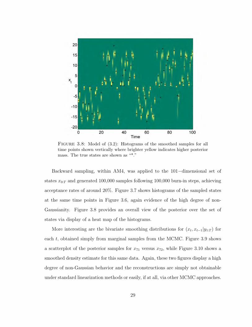
Figure 3.8: Model of (3.2): Histograms of the smoothed samples for alltime points shown vertically where brighter yellow indicates higher posteriormass. The true states are shown as “*.”
Backward sampling, within AM4, was applied to the 101−dimensional set of
states x0:T and generated 100,000 samples following 100,000 burn-in steps, achieving
acceptance rates of around 20%. Figure 3.7 shows histograms of the sampled states
at the same time points in Figure 3.6, again evidence of the high degree of non-
Gaussianity. Figure 3.8 provides an overall view of the posterior over the set of
states via display of a heat map of the histograms.
More interesting are the bivariate smoothing distributions for (xt, xt−1|y1:T ) for
each t, obtained simply from marginal samples from the MCMC. Figure 3.9 shows
a scatterplot of the posterior samples for x71 versus x72, while Figure 3.10 shows a
smoothed density estimate for this same data. Again, these two figures display a high
degree of non-Gaussian behavior and the reconstructions are simply not obtainable
under standard linearization methods or easily, if at all, via other MCMC approaches.
29

Figure 3.9: Model of (3.2): Scatterplot of MCMC samples for x71:72.
Figure 3.10: Model of (3.2): Reconstruction of bivariate densityp(x71,72|y1:100).
30

3.3.1 Effect of the number of components
As was illustrated in Section 3.2, the acceptance rate of the Metropolis algorithm
described in Chapter 2 is integrally tied to the number of components used in the
algorithm. As the number of components increases, the acceptance rate increases.
I now turn to the effect of the number of components on the acceptance rate in
the nonlinear model shown in equation (3.2). I perform the same analysis as in the
previous section, but now using half and double of the number of mixture components
used in the previous section. Each MCMC was initiated from the same initial value,
the final sample from the previous analysis, and run for 100, 000 iterations.
The overall acceptance over 100, 000 iterations was 0.8%, 9.2% and 32.3% for
500, 1,000, and 2,000 components, respectively. Figure 3.11 shows traceplots for
state x72 using varying number of components. This state was chosen for the multi-
modality it displays in the posterior, see Figure 3.10. This tri-modality is clear in
the traceplot using 2,000 components where one mode is centered around -10, one
around 0, and the last around 8. The traceplots indicate that both the 1,000 and
2,000 component proposals explore these three modes whereas 500 components is
insufficient. This model was chosen precisely because it is hard to estimate states
due to the nonlinearities involved. It is therefore unsurprising that a large number
of components are required to provide good approximations to these nonlinearities
and thereby provide a reasonable Metropolis acceptance probability.
3.3.2 Comparison to alternative MCMC schemes
In the previous section, the number of components used in the Metropolis proposal
was evaluated for its effect on acceptance probability and therefore the exploration of
the posterior distribution. In this section, I turn to alternative MCMC schemes that
do not require the linearization procedure used in AM4. In particular, I look at the
one state at a time (CPS) and multivariate random walk (MRW) approaches that
31

Figure 3.11: Traceplots for state x72 using 500, 1000, and 2000 com-ponents in the mixture filtering procedure from the top to the bottomrespectively.
were compared in Section 3.1. In that section, I noted that AM4 with J = 1, which
is equivalent to the FFBS algorithm, outperformed the CPS and MRW schemes in
terms of chain mixing in a DLM. In this section, I compare these algorithms on the
model shown in equation (3.2).
In the DLM example, CPS was available as a set of Gibbs steps which is not pos-
sible in this nonlinear example. Therefore, I perform a CPS random walk Metropolis
with tuning parameters such that the acceptance probability for each state is around
40%. Similarly I also used a MRW proposal with tuning parameter such that the
overall acceptance probability was around 20% (Gelman et al., 1996). Finally, I used
the AM4 method described in Chapter 2 using 1,000 components which was shown in
32

Figure 3.12: Traceplots for state x72 using CPS (green), MRW (blue),and AM4 (red) MCMC methods under approximately the same compu-tational time.
the previous section to have reasonable mixing properties. All chains were initialized
using the same value which was obtained by the final draw in a previous analysis
using the AM4 method.
For approximately equal computational times, I ran the AM4 method for 100,000
iterations achieving an acceptance rate around 12%, the CPS method for 300,000
iterations achieving acceptance rates with mean 47% and standard deviation of 4%,
and the MRW for 500,000 iterations achieving an acceptance rate around 21%.
Traceplots for state x72 for each analysis are provided in Figure 3.12. This figure
illustrates the concern with using either of the standard MCMC methods due to the
inability of those methods to effectively explore the posterior. This state appears to
33

have a tri-modal posterior according to Figure 3.10, but neither the CPS or MRW
approaches explore all three modes with this number of iterations. In contrast, the
AM4 method is able to explore the space effectively.
3.4 Summary
This chapter implements the adaptive mixture modeling Metropolis method devel-
oped in Chapter 2 on a number of nonlinear Gaussian models. Initially, I motivated
the necessity for joint state sampling by graphical illustration of Markov chain mix-
ing rates for standard MCMC approaches. I then looked at the effect of number
of mixture components and time series length on mixing via the Metropolis accep-
tance probability. Finally, I analyzed an illustrative nonlinear Gaussian model with
multi-modal state posterior comparing AM4 with standard MCMC methods. The
conclusion from this chapter is that joint sampling for the states can be necessary and
that the AM4 methodology is an effective way of accomplishing this for moderate
length time series.
More work is necessary to fully understand the efficiency gained by this approach.
Of interest would be theoretical research to determine whether the chain is uniformly
or geometrically ergodic. Initial attempts were made to look at this question using
results of Mengersen and Tweedie (1996), but no conclusive results have been ob-
tained. In addition, efficiency could certainly be improved by adaptively learning
the number of components required to obtain a good approximation to the filtering
density at each time point. These types of results would improve the computational
efficiency and therefore attractiveness of using the AM4 approach.
34

4
Parameter estimation in systems biology models
In some areas of systems biology investigators seek to build mathematical/statistical
models that describe the dynamics of protein concentrations within cells. Current
technological limits preclude measuring in vivo dynamics of protein concentrations
within cells. Therefore model systems are constructed in the closely related field
of synthetic biology. I begin this chapter by describing this field in Section 4.1
and thereby motivating the need for building models and estimating parameters
in biological systems. The current state of the art in measuring in vitro protein
concentrations is via time-lapse fluorescent microscopy discussed in Section 4.2. In
Section 4.3, I discuss approaches to building mathematical and statistical models for
these data ultimately developing a class of nonlinear dynamic models. Section 4.4
discusses MCMC methods for parameter and state estimation in these models. I
then analyze two different model systems in Sections 4.5 and 4.6.
35

4.1 Synthetic biology
Synthetic biology is a field devoted to creating living systems that perform a desired
task. For example, scientists may be interested in developing systems that perform
computations such as those described in my collaborative work with bioengineers
as reported in Tan et al. (2007), reproduced in Appendix F. The purpose of the
paper is to describe a bacterial system that can be used to perform mathematical
computations such as integration, optimization, and fast Fourier transforms. The
idea is to engineer a gene circuit that responds to a signal in a desired way. Bacterial
cells are transfected with this gene circuit to produce a living organism with a known
response to environmental signals. Placing these engineered bacteria into the proper
environment allows us to read a response from these bacteria. For example, scientists
may be interested in the level of some pollutant in a remote area. Bioengineers could
build bacteria to fluoresce in the presence of this pollutant, drop the bacteria in by
plane, and read a response by satellite. Since this is a living organism, a response
could be read over time as the pollutant level fluctuates.
Statistical methods can aid such studies by improving the understanding of how
bacteria will respond to a given stimulus. In particular, scientists may be interested
in understanding a dose-response curve, e.g. fluorescence as a function of level of
pollutant, or dynamic model parameters. Engineering of these circuits will inevitably
require multiple cycles of design and testing. Statistical methods and, in particular,
Bayesian methods are suited to help in defining where existing knowledge is present
about aspects of the circuit design and where more knowledge is needed. Using these
methods, statisticians can suggest experimental designs that further understanding
of the relevant biochemistry and thereby decrease the number of design cycles as well
as the overall design time. Using Bayesian methods provides a natural framework for
iteratively gaining knowledge about model parameters, e.g. biochemical parameters,
36

in each step of the design. In addition, understanding these biochemical parameters
will lead to more accurate inferences when performing real-world computations such
as measuring pollution.
4.2 Time-lapse fluorescent microscopy experiments
Recent technological advances allow for reporting of in vitro measurements of pro-
teins via fluorescent proteins (FPs). Initially purified from the jellyfish Aequorea
victoria as green fluorescent protein by Shimomura et al. (1962), this protein has
been mutated to produce a variety of emission wavelengths, e.g. yellow fluorescent
protein and cyan fluorescent protein (CFP) (Tsien, 1998). Varying the emission
wavelengths allows multiple FPs to be measured simultaneously. Each fluorescent
protein is distinguished by its absorption and emission spectra (Patterson et al.,
2001) which determine the optimal wavelengths used to excite and measure each of
the proteins. These fluorescent proteins have become so important that the 2008
Nobel Prize in chemistry was given for their discovery and development.
These proteins have been introduced into living organisms such as in root studies
in the plant Arabidopsis (Brady et al., 2007) and in the bacterium Escherichia coli
(Rosenfeld et al., 2005; Pedraza and van Oudenaarden, 2005). Bacteria are extremely
convenient organism for transfection with FPs since they are translucent, which
allows easy study of cellular dynamics in vitro. In bacteria, the typical approach is
to design a gene circuit on a plasmid and then transfect the bacterial cells with this
plasmid (Tu et al., 2007). The gene circuit (or circuits) will contain one or more
fluorescent proteins that will provide a means of obtaining measurements on the
bacterial system. In order for the gene circuit to function properly it must borrow
machinery from the bacterial environment - such as DNA replication, DNA to RNA
transcription, and RNA to protein translation.
The transfected bacteria are placed on a microscope slide in survivable medium.
37

A light source is used to excite the fluorescent protein of interest and a digital cam-
era measures the resulting emission. Emission is measured as an 8-bit number and
therefore fluorescence is measured on a scale from 0 to 255, which will be important
when assigning priors to model parameters in Section 4.5.1. Equipment is available
to automate the task of lighting and photography which allows for hands-free data
collection. Ideally, the time resolution of measurements should be very fine so that a
detailed understanding of the cellular dynamics can be ascertained. Unfortunately,
(semi-)continuous exposure to light causes destruction of fluorophores, the compo-
nents responsible for fluorescence, in a process called photobleaching (Tsien, 1998).
Therefore, the standard time resolution for experiments of this type is 10 minutes.
Time-lapse fluorescent microscopy experiments have been used effectively to mea-
sure some biochemical and measurement parameters. Rosenfeld et al. (2005) estimate
biochemical parameters in a repression system, Pedraza and van Oudenaarden (2005)
estimate the amount of variability due to small copy numbers and integer number
of reactions compared to variability due to environmental conditions, intrinsic and
extrinsic noise respectively, and Rosenfeld et al. (2006) estimate the amount of fluo-
rescence per molecule. Analyses such as these, and the one presented here, begin to
reveal details of the dynamics of the cellular environment.
4.3 Modeling chemical reactions
Many approaches at building mathematical/statistical models for biochemical sys-
tems have been proposed. This section highlights a few of those approaches including
deterministic chemical kinetics, stochastic chemical kinetics, diffusions, and discrete-
time models. All of these approaches model a biochemical system composed of a
set of species and reactions. Species comprise the molecules of interest that could
possibly be observed if the appropriate equipment were available. These species un-
dergo chemical reactions that can produce species, degrade species, or convert one (or
38

more) species to another. For theoretical reasons, the biochemical system is usually
assumed to be in thermal equilibrium in some fixed volume V , see Gillespie (1977).
Biologists would prefer estimation of the reaction rates discussed below, but, as will
be discussed, only complicated functions of these rates are able to be estimated. This
section continues by first introducing a more technical description of a biochemical
system and then briefly discussing these alternative modeling approaches in order to
derive the discrete-time biological model used for statistical analysis.
4.3.1 Biochemical system
Consider a biochemical system involving K species X1, X2, . . . , XK and P reactions
labeled R1, R2, . . . , RP . The biochemical system can be described in the following
form
R1 : u11X1 + u12X2 + · · ·+ u1KXK → v11X1 + v12X2 + · · ·+ v1KXK
R2 : u21X1 + u22X2 + · · ·+ u2KXK → v21X1 + v22X2 + · · ·+ v2KXK
...
RP : uP1X1 + uP2X2 + · · ·+ uPKXK → vP1X1 + vP2X2 + · · ·+ vPKXK
where upk ∈ N = 0, 1, . . . and vpk ∈ N indicate in reaction p the number of
molecules of species k consumed and produced, respectively.
4.3.2 Deterministic chemical kinetics
Reaction Rp has a deterministic reaction rate rp given by
rp = − 1
upk
d[Xk]
dt=
1
vpk
d[Xk]
dt= kp(T )[X1]
up1 [X2]up2 · · · [XK ]upK
where [Xk] indicates concentration of species Xk and kp(T ) is the reaction rate coef-
ficient that depends on the temperature T . The reaction rate rp depends only on the
species to the left of → in the set of reactions described above. Note that if upk = vpk
39
then no change is observed in species k even though this species may be involved in
the rate of the reaction, e.g. catalysts. For each individual species in the system,
the change in its concentration is given by d[Xk]dt
=∑P
p=1 apkrp where apk = vpk−upk.
This provides a set of k coupled ordinary differential equations that may describe
the dynamics of the system (IUPAC, 1997).
Even in very simple settings, the number of elementary reactions can be ex-
tremely large. One way of reducing the dimensionality is the quasi-steady state
assumption (QSSA). This assumption sets the reaction rates for particular reactions
to zero and then solves the set of equations to remove some of the species from the
model. The QSSA will be approximately correct in situations where some reactions
occur much faster than others and therefore come to an equilibrium quickly, i.e. the
multiscale problem Ferreira et al. (2006); Ferreira and Lee (2007). The QSSA in
general will introduce nonlinearities into the differential equations for the remaining
species. Therefore parameter estimation in these types of models is often accom-
plished through a nonlinear least-squares fit to the data (Connors, 1990; Farinha
et al., 1997).
Deterministic chemical kinetics assume chemical species are evolving in contin-
uous space and deterministically. This is unrealistic since molecules are discrete
quantities. Nonetheless when species quantities are large, this assumption is accu-
rate. In biological applications the quantities can be as small as one or two and
therefore violate the assumption severely. Similarly, the chemical species are not
evolving deterministically, but rather are the result of the stochastic process of reac-
tion occurrences. Relaxing of these assumptions led to the development of stochastic
chemical kinetics.
40
4.3.3 Stochastic chemical kinetics
Considering the same biochemical system described in Section 4.3.1, reaction Rp
has a stochastic reaction rate cp and hazard hp(X, cp) (Golightly and Wilkinson,
2005; Wilkinson, 2006) where X represents the current number of molecules for each
species. In thermal equilibrium in a fixed volume, Gillespie (1977) derived the form
of the hazard function such that hp(X, cp)∆t is the probability of reaction p occurring
in the small time interval ∆t. With P reactions, this provides a hazard that at least
one reaction occurs in this time interval, namely h0(X, c) =∑P
p=1 hp(X, cp) where
c = c1, c2, . . . , cp. Therefore a continuous time, discrete state-space simulation
method is readily available by choosing a reaction time τ ∼ Exp(1/h0(X(t), c)),
an exponential random variable with mean 1/h0(X(t), c), and a reaction indicator
q with probability proportional to hp(X(t), cp), q ∈ 1, 2, . . . , P (Gillespie, 1977).
Time is incremented by τ and the number of molecules of each species is updated
via Xk(t+ τ) = Xk(t) + aqk. More sophisticated algorithms and approximations are
described in Gillespie (2007). Simulations based on this stochastic chemical kinetic
approach are performed in Section 4.5.3.
With perfect knowledge of the system, i.e. knowing X(t) for all t ∈ (0, T ),
stochastic reaction rates can be inferred easily. Unfortunately in the more realis-
tic scenario of perfect but discrete observations of the system, the problem becomes
analytical intractable and, even worse, numerical techniques are challenging (Wilkin-
son, 2006). This challenge comes from the necessity to simulate paths from X(ti)
to X(ti+1) where ti and ti+1 are consecutive observation times (Boys et al., 2008).
Therefore, at the current time, using statistical procedures to estimate stochastic
chemical kinetic parameters in biological systems is not practical.
41

4.3.4 Chemical Langevin equation
One approach to approximating stochastic chemical kinetics advocated by Wilkin-
son uses stochastic differential equations (SDEs), or diffusions, to approximate the
stochastic chemical kinetic equations. The general form of these SDE models is
dXt = µ(Xt)dt+ σ(Xt)dWt (4.1)
where Xt is K-vector representing the amount of each species at time t, µ(Xt)dt
is a K-vector describing the mean change in Xt over time interval dt, dWt is the
increment of a Wiener process with variance parameter dt, and σ(Xt) accounts for
the magnitude and correlation in the evolution of Xt due to the system of reactions.
In this context, equation (4.1) is known as the chemical Langevin equation. Matching
the mean and variance yields the approximation µ(Xt) = Sh(Xt, c) and σ(Xt) =
S diag√h(Xt, c) where S is the transpose of A = apk and diagh is the diagonal
matrix with elements h. This yields a driving Wiener process that has dimension
P different from the dimension K of Xt. Typically, P > K and the approximation
can be re-written with a Wiener process of dimension K, see (Wilkinson, 2006, Ch.
8) for discussion. Note that setting dWt to zero recovers the ordinary differential
equation model discussed in Section 4.3.2.
The reason for introducing this SDE is to allow for statistical parameter estima-
tion. Progress has been made in some SDEs (Beskos et al., 2006), but parameter
estimation in these models is, in general, an unsolved problem. A common approach
for these models is to make an approximation to the SDE using a sufficiently small
time-step (h = 1/H) such that the Euler-Maruyama approximation is valid, i.e.
Xt+h|Xt ≈ N(Xt + µ(Xt)h, σ(Xt)h). (4.2)
Markov chain Monte Carlo (MCMC) analysis can then be performed on the resulting
difference equation based model. If the system is observed at discrete time intervals
42

t ∈ 1, 2, . . . , T, then this involves alternating between sampling for the parameters,
θ = c1, c2, . . . , cP, and the unobserved states, Xt+h, Xt+2h, . . . , Xt+1−h for t ∈
1, 2, . . . , T − 1. Sampling for the parameters requires Metropolis-Hastings steps
since the parameters are involved in both the mean and the variance of the difference
equation. If the system is observed with measurement error, then the sampling of
all states, Xt : t ∈ 1, 2, . . . , TH is required and performed conditional on both
the parameters and the observed data. A discussion of this approach is available in
Golightly and Wilkinson (2005) and sequential approaches are discussed in Golightly
and Wilkinson (2006a,b)
4.3.5 Dynamic nonlinear models
The above chemical kinetic modeling techniques are appropriate when measurements
are taken on many of the species in the system. In practice this is often not the case.
In the example described later, measurements are made on only one of the four
species in the biochemical system. Some simulation studies have been conducted to
understand partial observation of the system, e.g. Golightly and Wilkinson (2006b,
2008), but relative to a real-world system, even these partial observations are ambi-
tious.
Consider a context where a specified system of reactions is believed to govern
the dynamics of a system. This context appears in both the fields of synthetic
biology, where a reaction system is actually created and placed in an organism, as
well as systems biology, where extensive high-throughput gene expression studies
have identified the way in which species interact. This system can be approximated
by a diffusion that is similar in form to equation (4.1), but replaced the mean and
covariance with an approximation that borrow from both deterministic and stochastic
modeling frameworks.
For parameter estimation, I adopt the approach of Golightly and Wilkinson (2008)
43

and approximate the SDE by a difference equation given by the Euler-Maruyama
approximation. These models include measurement error and therefore the resulting
model for time-lapse fluorescent microscopy measurements can be written in dynamic
form. Including multiple independent cells in the analysis provides the dynamic
model
yc,t = f(xc,t|θc) + νc,t, (4.3a)
xc,t+h = g(xc,t|θc) + ωc,t, (4.3b)
where yc,t and xc,t are is the observed and true amount of all species in cell c at
time t, νc,t ∼ N(0, σ2mI) and ωc,t ∼ N(0, hΣ) and independent across time and
mutually independent, θc are fixed parameters governing the nonlinear equations
in the observation and evolution equations. I use the terminology cell trajectory
to mean the sequence of observations yc,1:T following one cell through time. Since
observations are taken on one scale, but this scale is sub-divided into H subintervals,
many of the yc,t will be unobserved.
4.4 Parameter estimation
Unknown quantities are estimated using MCMC methods by alternating draws from
parameters given states followed by states given parameters. When available, I
choose conditionally conjugate priors for model parameters, i.e. inverse gamma or
inverse Wishart distributions for variance parameters and Gaussian distributions for
linear parameters in equations (4.3). The parameters in the nonlinear functions are
multiplications and divisions of chemical kinetic parameters, which are all positive,
and therefore, truncated Gaussian priors are used for these parameters. Due to the
intractability of the full conditional distributions of multivariate truncated Gaussians
(Philippe and Robert, 2003), I perform sampling on univariate parameters. For
parameters that are not linear in equations (4.3), I use random walk Metropolis
44

methods.
Sampling from states conditional on parameters is trivial when the states occur
linearly in equations (4.3) since sampling can be performed exactly using the forward
filtering backward sampling algorithm (Carter and Kohn, 1994; Fruhwirth-Schnatter,
1994). In general, the states will occur nonlinearly in these equations. Sampling can
proceed using Metropolis methods on individual states (Carlin et al., 1992). Due to
high correlation between the states, these methods can suffer from poor mixing as
was shown in Chapter 3. To increase mixing, the method of Chapter 2 is used. Its
application under subintervals and therefore missing data is described below.
Consider the generic dynamic model shown in equations (4.3) where, for simplic-
ity, I drop the conditioning on θc as well as the subscript c, since cells are independent.
I build a joint Metropolis proposal for all states based on analytical approximations
to the filtering and smoothing distributions. In the algorithm, I say ‘regenerate f(x)
to obtain Nm(p1:J ,m1:J , C1:J)’ to mean the procedure outlined in Table 2.1. The
Metropolis proposal is then built by first performing the deterministic adaptive mix-
ture filtering shown in Table 4.1. Repeating this procedure for t ∈ 1, 2, . . . , TH
provides analytical approximations to the filtering distributions. Since many obser-
vations are missing, the algorithm is simplified since the posterior is equal to the
prior at those time points.
To obtain a draw from the joint distribution of all latent states, backward sample
from the mixtures using the procedure described in Table 4.2. Since this proce-
dure only provides an approximate draw from the desired distribution, a Metropolis-
Hastings step is performed using this draw as a proposal. The Metropolis-Hastings
acceptance probability can be calculated according to equation (2.10).
45

Table 4.1: Beginning with a filtering density at time t − h, namely p(xt−h|y1:t−h) =Nm(pt−h,1:J ,mt−h,1:J , Ct−h,1:J), this adaptive mixture filtering algorithm provides arecursive procedure to calculate the filtering density at time t.
1. Calculate an approximation to the prior
p(xt|y1:t−h) ≈ Nm(pt−h,1:J , at,1:J , Rt,1:J)
where
at,j = g(mt−h,j) and Rt,j = (g′(mt−h,j))2Ct−h,j + σ2mt−1,jh
2. Regenerate p(xt|y1:t−h) to obtain Nm(pt−h,1:J , at,1:J , Rt,1:J). If yt is unobserved,
set pt,j = pt−h,1:J , mt−h,1:J = at−h,1:J , Ct−h,1:J = Rt−h,1:J and skip to step 5.
3. Calculate an approximation to the one step ahead prediction
p(yt|y1:t−h) ≈ Nm(pt−h,1:J , ft,1:J , Qt,1:J),
where
ft,j = f(at,j) and Qt,j = (f ′(at,j))2Rt,j + σ2
m.
4. Calculate an approximation to the posterior
p(xt|y1:t) ≈ Nm(pt,1:J , mt,1:J , Ct,1:J)
where
mt,j = at,j + At,jet,j, Ct,j = Rt,j + A2t,jQt,j,
et,j = yt − ft,j, At,j = Rt,jf′(at,j)/Qt,j,
pt,j ∝ pt−1,jN(yt|ft,j, Qt,j).
5. Regenerate p(xt|y1:t) to obtain Nm(pt,1:J ,mt,1:J , Ct,1:J)
46

Table 4.2: Backward sampling from an adaptive mixture filter generated accordingto Table 4.1.
1. Draw xT ∼ Nm(pT,1:J ,mT,1:J , CT,1:J) and set t = T − h.
2. Calculate the component probabilities, means, and variances for the distribu-tion p(xt|xt+h, yt) = Nm(qt,1:J , ht,1:J , Ht,1:J) where
ht,j = mt,j +Bt,j(xt+h − at+h,j) and Ht,j = Ct,j −B2t,jRt+h,j
Bt,j = Ct,jg′(mt,j)/Rt+h,j and qt,j ∝ pt,jN(xt+h|at+h,j, Rt+h,j)
3. Draw xt ∼ Nm(qt,1:J , ht,1:J , Ht,1:J). If t > 0, set t = t− h and return to Step 2.
4.5 Feedback of T7 RNA polymerase
This system is defined by the seven reactions shown in Table A.1. The derivation
from these seven reactions to a differential equation model is shown in Appendix A.
As described in Section 4.3.5, to build a statistical model for these data, I take the
Euler-Maruyama discretization of this differential equation and add measurement
and evolution error to form the DnLM
yc,t = xc,t + νc,t, (4.4a)
xc,t = xc,t−1 +kc + αcxc,t−1
βc + xc,t−1
− dcxc,t−1 + ωc,t, (4.4b)
where νc,t ∼ N(0, V ) and ωc,t ∼ N(0,W ) are independent across time and cell
and mutually independent of each other. The unknown fixed parameter set is
θ = kc, αc, βc, dc, V,W for c ∈ 1, 2, . . . , C. The subscript c indicates that each
cell evolves independently and according to evolution equations with different param-
eters. The attempt in the subsequent analyses are to distinguish cells on the basis
of the parameters defining their evolutions. Therefore identical priors are placed on
equivalent parameters for different cells, e.g. p(kc) = p(kc′) for c 6= c′. The follow-
47
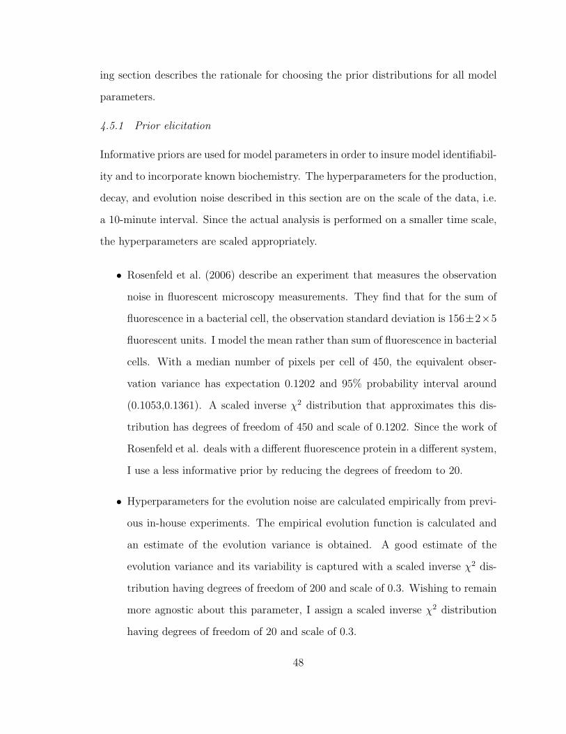
ing section describes the rationale for choosing the prior distributions for all model
parameters.
4.5.1 Prior elicitation
Informative priors are used for model parameters in order to insure model identifiabil-
ity and to incorporate known biochemistry. The hyperparameters for the production,
decay, and evolution noise described in this section are on the scale of the data, i.e.
a 10-minute interval. Since the actual analysis is performed on a smaller time scale,
the hyperparameters are scaled appropriately.
• Rosenfeld et al. (2006) describe an experiment that measures the observation
noise in fluorescent microscopy measurements. They find that for the sum of
fluorescence in a bacterial cell, the observation standard deviation is 156±2×5
fluorescent units. I model the mean rather than sum of fluorescence in bacterial
cells. With a median number of pixels per cell of 450, the equivalent obser-
vation variance has expectation 0.1202 and 95% probability interval around
(0.1053,0.1361). A scaled inverse χ2 distribution that approximates this dis-
tribution has degrees of freedom of 450 and scale of 0.1202. Since the work of
Rosenfeld et al. deals with a different fluorescence protein in a different system,
I use a less informative prior by reducing the degrees of freedom to 20.
• Hyperparameters for the evolution noise are calculated empirically from previ-
ous in-house experiments. The empirical evolution function is calculated and
an estimate of the evolution variance is obtained. A good estimate of the
evolution variance and its variability is captured with a scaled inverse χ2 dis-
tribution having degrees of freedom of 200 and scale of 0.3. Wishing to remain
more agnostic about this parameter, I assign a scaled inverse χ2 distribution
having degrees of freedom of 20 and scale of 0.3.
48

• Decay in mean fluorescence is composed of both the protein decay and increase
in pixel size of a bacterial cell. The decay of T7 RNAP has a half-life around
4 hours [Cheemeng Tan, personal communication]. The percentage increase
in pixel size of a bacterial cell was estimated using previous experiments and
found to be 7.4% in a 10-minute period. Combining these two effective decay
rates, I find the overall percentage decay to have an expected value of 0.0952
over a 10-minute period. As a prior for this parameter, I use a normal truncated
to (0,1) with expected value 0.0952 and scale parameter .01.
• The parameter k, which accounts for the production of T7 RNAP when no
T7 RNAP is available for the feedback loop, is small but it is unclear how
small. Previous attempts at modeling this data with diffuse priors on this
parameter caused identifiability issues since either αx or k can be responsible
for production. Therefore, I use an informative prior on this parameter based on
scientific intuition. The resulting prior is a positive normal prior with expected
value of 0.1 and standard deviation 0.1.
• The parameter α accounts for the level of production of T7 RNAP when the
level of T7 RNAP is high. Since I have placed an informative prior on k less
information is needed about α in order to insure identifiability of the model.
I use a diffuse positive normal prior with expected value of 4 and standard
deviation of 10.
• Finally, the nonlinear parameter β represents the equilibrium constant for the
binding and unbinding of T7 RNAP association with the promoter. As a
practical matter, it is hard to measure this equilibrium constant. Even if it
were, I am modeling the changes of protein concentration on the fluorescence
level and the conversion factor is unknown. Attempting to be non-informative
49

I assume a positive normal prior with mean of 10 and standard deviation of
10.
In the model described by equations (4.4), parameters describing the evolution
function for each cell trajectory are distinct. In the analyses that follow, the equiva-
lent prior distributions are assumed for the same parameters in each cell trajectory
and the observed differences between the posterior distributions inferred by each tra-
jectory is analyzed. More information on priors and full conditional distributions is
available in Appendix C.1.
4.5.2 DnLM simulated data
As a first approach to understand parameter estimation in discrete-time biological
models, simulations from the model shown in equations (4.4) were performed for
C = 2. For the two cell trajectories the following parameters were used: k = 0.01,
β = 10, d = 0.01, W = 0.3, V = 0.12 and x1,0 = x2,0 = 50. The trajectories differed
only in the α parameter where that parameter was set to 0.25 and 1.2 to represent
low and high T7 feedback mechanisms, respectively. The results of this simulation
are shown in Figure 4.1 where the effect of α is clear.
Figure 4.2 shows the results of an MCMC analysis using J = 1 components in
AM4 with p(x1,0) = p(x2,0) = N(50, 1). As can be seen from the plots, no new
information is gained in the analysis about the parameters k1, k2, β1, β2, and V , but
information is gained on α1, α2, d1, d2, and W . Importantly, the information gained
on the decay parameter is consistent between the two sets of cells but the posteriors
for α, the feedback production term, hardly overlap. Recall that the only difference
in the two sets of simulated data is in that parameter noted by the two red Xs in
the upper right hand plot of the figure.
The production and decay parameters are highly correlated as can be seen in
Figure 4.3. This correlation should be unsurprising because an increase in decay can
50

Figure 4.1: Time-lapse fluorescent microscopy data simulated from aDnLM for two levels of enhanced RNA production. The shaded regions in-dicate 95% probability intervals based on 1,000 simulations from the modelwhile the two trajectories are the simulations used in this analysis.
be compensated for by an increase in the production. This correlation is important
when building new biochemical models and thinking about priors on parameters in
those models. For identifiability reasons, informative priors will be needed on at
least one of the parameters. In order to obtain meaningful information separately on
these parameters, experiments need to be designed to isolate one of the parameters.
The decay rate is easier to isolate by designing an experiment that has no produc-
tion but only has decay of the protein. In the literature, this is the case as more
information is available on decay rates than on most other biochemical parameters,
see e.g. Rosenfeld et al. (2006).
In addition to posterior estimates of fixed biochemical parameters, the MCMC
analysis also provides posterior estimates for the latent protein levels. Figure 4.4
shows posterior estimates of the two cell trajectories shown in Figure 4.1. The
51

Figure 4.2: Posterior plots for model parameters based on the DnLMsimulated data shown in Figure 4.1. The top four plots contain posteriorhistograms for cells with low (red) versus high (blue) enhanced RNAproduction. Starting from the top left and continuing clockwise, theseparameters are k, α, β, and d. The bottom two plots show parameterscommon to both sets of cells where
√W is shown on the left and
√V
shown on the right. In all plots, the prior is shown in green and thetruth shown as a red X.
pointwise 95% credible intervals display a characteristic linked-bubble shape due to
the imputation of latent states between observations. The locations of the link in
these bubbles is due to an observation occurring at that time and therefore more
information is available for the posterior estimate of that latent state. Similarly, the
least information about the latent state is available mid-way between observations
and therefore the credible interval has maximum width at those times.
52
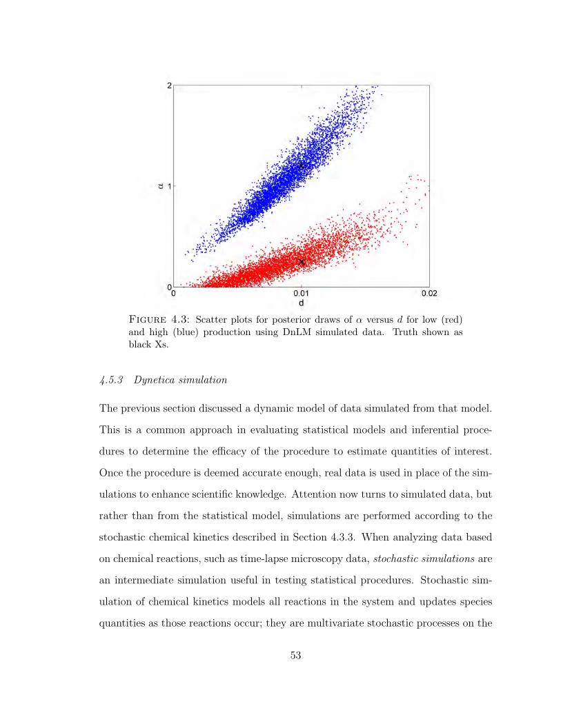
Figure 4.3: Scatter plots for posterior draws of α versus d for low (red)and high (blue) production using DnLM simulated data. Truth shown asblack Xs.
4.5.3 Dynetica simulation
The previous section discussed a dynamic model of data simulated from that model.
This is a common approach in evaluating statistical models and inferential proce-
dures to determine the efficacy of the procedure to estimate quantities of interest.
Once the procedure is deemed accurate enough, real data is used in place of the sim-
ulations to enhance scientific knowledge. Attention now turns to simulated data, but
rather than from the statistical model, simulations are performed according to the
stochastic chemical kinetics described in Section 4.3.3. When analyzing data based
on chemical reactions, such as time-lapse microscopy data, stochastic simulations are
an intermediate simulation useful in testing statistical procedures. Stochastic sim-
ulation of chemical kinetics models all reactions in the system and updates species
quantities as those reactions occur; they are multivariate stochastic processes on the
53

Figure 4.4: Posterior 95% credible intervals (blue) for the latent stateseries with the truth (red) for DnLM simulated data.
positive integers in continuous time. For a review, see Gillespie (2007).
Stochastic simulations were performed using the Dynetica software (You et al.,
2003) according to the first reaction method (Gillespie, 1977). Dynetica is a graphi-
cal user interface that allows for building biochemical systems according to species,
reactions, and reactions rates (either deterministic or stochastic). It allows for deter-
ministic simulations according to approximations to the differential equations as well
as stochastic simulations using a variety of methods. Figure 4.5 displays the Dynet-
ica schematic used in this simulation. This schematic is a graphical representation
of the biochemical system under study.
Data were recorded on 10-minute intervals for a total of 400 minutes. The kinetic
parameters used in this simulation are 0.001 for basal RNA production, 1 for protein
production, 5.6 and 0.2 for association and dissociation of protein with the promoter,
0.063 for RNA decay, and 0.00435 for protein decay. Simulations were performed
54

Figure 4.5: Dynetica schematic of T7 RNA polymerase feedback. Thefour chemical species (blue circles) either decay (red lines) or are pro-duced (green lines) through a set of seven chemical reactions (boxes witharrows) described in Table A.1.
using two different levels of enhanced RNA production: 0.005 (low) and 0.24 (high).
The simulations were initiated with 50 T7 genes (multiplicity due to the number
of plasmids within the cell containing this gene circuit), 1500 T7 protein molecules,
no RNA, and no promoter-protein complexes, but only the number of T7 protein
molecules is recorded. The quantity of T7 RNAP protein was then multiplied by
15, representing the conversion to fluorescence units (Rosenfeld et al., 2006), and
divided by 450 to obtain mean fluorescence per pixel. The simulated data are shown
in Figure 4.6. Measurement noise was then added as independent Gaussian errors
with mean 0 and variance 0.12.
Figure 4.7 displays MCMC estimates of the parameters in equations (4.4) on
Dynetica simulated data using exactly the same priors and tuning parameters as
in the previous section. Similar to the previous analysis, no information gain is
seen for parameters k1, k2, β1, β2, and V although perhaps V has a slight shift. In
contrast, the parameters α1, α2, d1, d2, andW are informed by the data. In particular,
55

Figure 4.6: Dynetica simulated time-lapse fluorescent microscopy data fortwo levels of enhanced RNA production. The shaded regions indicate 95%probability intervals based on 1,000 simulations from the model while the twotrajectories are the simulations used in this analysis.
interest focuses on the posterior for parameter α1 compared to α2 since the system
was simulated expecting these two parameters to be different. The posteriors are
certainly different for these two parameters, but not as distinctly as in the DnLM
simulated data. It appears the difference in these parameters is perhaps confounded
with the observed difference in the posterior for the decay parameters.
Figure 4.8 shows the posterior correlation for the enhanced production and decay
parameters for the two analyses. It is clear from this figure that the posterior joint
distribution for these two parameters lie in different regions of the parameter space.
The fan shape of the joint distribution for these parameters under the high production
simulation suggests using a more informative prior for at least one of the parameters
when possible.
Figure 4.9 displays 95% credible intervals for the latent state. These posterior
56

Figure 4.7: Posterior plots for model parameters based on Dyneticasimulated data shown in Figure 4.6. The top four plots contain pos-terior histograms for cell trajectories with low (red) versus high (blue)enhanced RNA production. The bottom two plots show parameterscommon to both sets of cell trajectories. In all plots, the prior is shownin green. The true parameter value is known only for
√V and is shown
as a red X in that plot.
estimates are useful when studying a cascading network where the levels of upstream
proteins affect the levels of downstream proteins. In particular, a common view is
that biological systems work on thresholds whereby a downstream protein becomes
active when an upstream protein reaches a threshold. If the threshold for this protein
happened to be 100, the data alone would suggest the protein reaches that level at
time 250, but the statistical analyses suggests that there is a sizable probability that
it occurs between time 240 and 250, with some smaller probability that it occurs
57

Figure 4.8: Scatter plots for posterior draws of α versus d for low (red)and high (blue) production using Dynetica simulated data.
before time 240.
4.5.4 Time-lapse fluorescent microscopy data
Escherichia coli bacteria were transfected with a plasmid containing a gene circuit.
This gene circuit contains a T7 RNAP gene and the cyan fluorescence protein (CFP)
gene. The circuit is constructed such that T7 RNAP and CFP are simultaneously
expressed and therefore CFP is a measure of the amount of T7 RNAP in the sys-
tem. A small number of these bacterial cells were placed on a microscope slide and
photographed automatically on 10-minute intervals; see Section 4.2 for more details
of time-lapse microscopy experiments. Figure 4.10 shows three frames from a time-
lapse microscopy movie. The phase image in this figure uses all visible light and is
therefore exactly what a scientist would see while looking through the microscope.
The fluorescent image on the other hand is produced by shining light of 455nm in
58

Figure 4.9: Posterior 95% credible intervals (blue) for the latent stateseries with the truth (red) for Dynetica simulated data.
wavelength and then recording the intensity of light at wavelength 480 ± 40 for a
short duration.
Cell segmentation, tracking, lineage reconstruction, and data collection were per-
formed using CellTracer (Wang et al., 2009); this paper, describing our novel imaging
methodology, is reproduced in Appendix E. The main contributions of the paper in-
clude an algorithm for automatically identifying individual cells in a population,
tracking each cell from one frame to the next as well as multiple daughter cells from
one mother cell, building a genealogic tree to record which daughter cells are descen-
dent from which mother cells, and reporting cell characteristics such as fluorescence
level and size. CellTracer outperforms other commercially and academically available
software for these tasks in bacterial cells as well as in other contexts.
My contribution to the work involved testing alternative software and discussions
involving the algorithm design. Prior to building the software in house, I attempted
59

Figure 4.10: Frames from a time-lapse fluorescent microscopy movie.The phase image contains all wavelengths of visible light whereas the flu-orescence image is captured using a filter that only records wavelengthsaround 480nm.
to find existing commercial or academic software, but none produced satisfactory
results. Some of the algorithm innovations in CellTracer include novel methods
for iterative removal of the background from the segmentation process, performing
the segmentation through iterations of filtering, tracking cells through time using
overlapping both forward and backward in time, and modeling cells as “bendy”
cigars.
Figure 4.11 shows the resulting fluorescence trajectory of two cells that appear
to have different biochemical parameters. There is no immediate reason as to why
two cells would have similar fluorescence up to time 200 and diverge thereafter.
Therefore, it is assumed for the purposes of this analysis that the similarity up to
time 200 is solely due to the random, intrinsic noise in the cellular environment of
the cells.
Similar to the previous analyses, this data was analyzed using the model of equa-
60

Figure 4.11: Mean cellular fluorescence in two cells obtained using time-lapse fluorescent microscopy on 10-minute intervals.
tions (4.4) and exactly as performed in the previous two sections. Figure 4.12 displays
posterior histograms for model parameters estimated using time-lapse microscopy
data. Compared to the simulated data, in this analysis the evolution variance as
well as the enhanced production and decay parameters are informed by the data.
The enhanced production parameters have distinctive posterior distributions due to
their shapes, but it is unclear if this is suggesting that one has higher or lower produc-
tion than the other. In contrast, the decay parameters appear to be different. The
decay parameter for the high trajectory in Figure 4.11 is small compared to the de-
cay parameter for the low trajectory. This lends credence to the scientific hypothesis
raised that bistability in protein fluorescence level is caused by growth-modulation
[Cheemeng Tan, personal communication].
Figure 4.13 shows the posterior correlation between the α and d parameters for
the two different cell trajectories. On one hand, the marginal distribution for α shown
61

Figure 4.12: Posterior plots for model parameters based on real datashown in Figure 4.11. The top four plots contain posterior histogramsfor cell trajectories with low (red) versus high (blue) enhanced RNAproduction. The bottom two plotsshow parameters common to bothsets of cell trajectories. In all plots, the prior is shown in green.
in Figure 4.12 suggests there is not enough information in the data to distinguish the
parameter α between the two trajectories. On the other hand, this bivariate scatter
plot suggests that it is the joint distribution of α and d that are distinct.
Figure 4.14 then shows posterior credible intervals for the latent protein state.
The large jump in the blue trajectory around time 340 suggests a heavier-tailed
distribution to govern the underlying dynamics. In particular, modeling the evolution
using any Beta-Gamma autoregressive process (Ristic, 2005) would provide for this
dynamic.
62
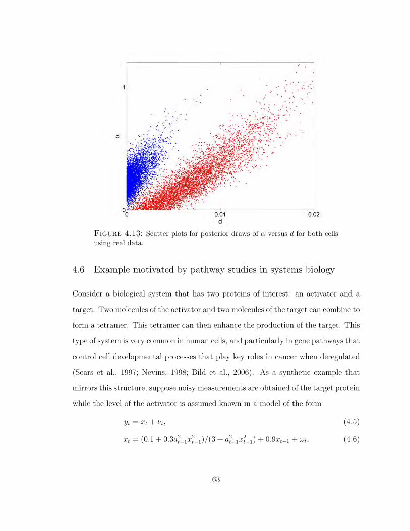
Figure 4.13: Scatter plots for posterior draws of α versus d for both cellsusing real data.
4.6 Example motivated by pathway studies in systems biology
Consider a biological system that has two proteins of interest: an activator and a
target. Two molecules of the activator and two molecules of the target can combine to
form a tetramer. This tetramer can then enhance the production of the target. This
type of system is very common in human cells, and particularly in gene pathways that
control cell developmental processes that play key roles in cancer when deregulated
(Sears et al., 1997; Nevins, 1998; Bild et al., 2006). As a synthetic example that
mirrors this structure, suppose noisy measurements are obtained of the target protein
while the level of the activator is assumed known in a model of the form
yt = xt + νt, (4.5)
xt = (0.1 + 0.3a2t−1x
2t−1)/(3 + a2
t−1x2t−1) + 0.9xt−1 + ωt, (4.6)
63
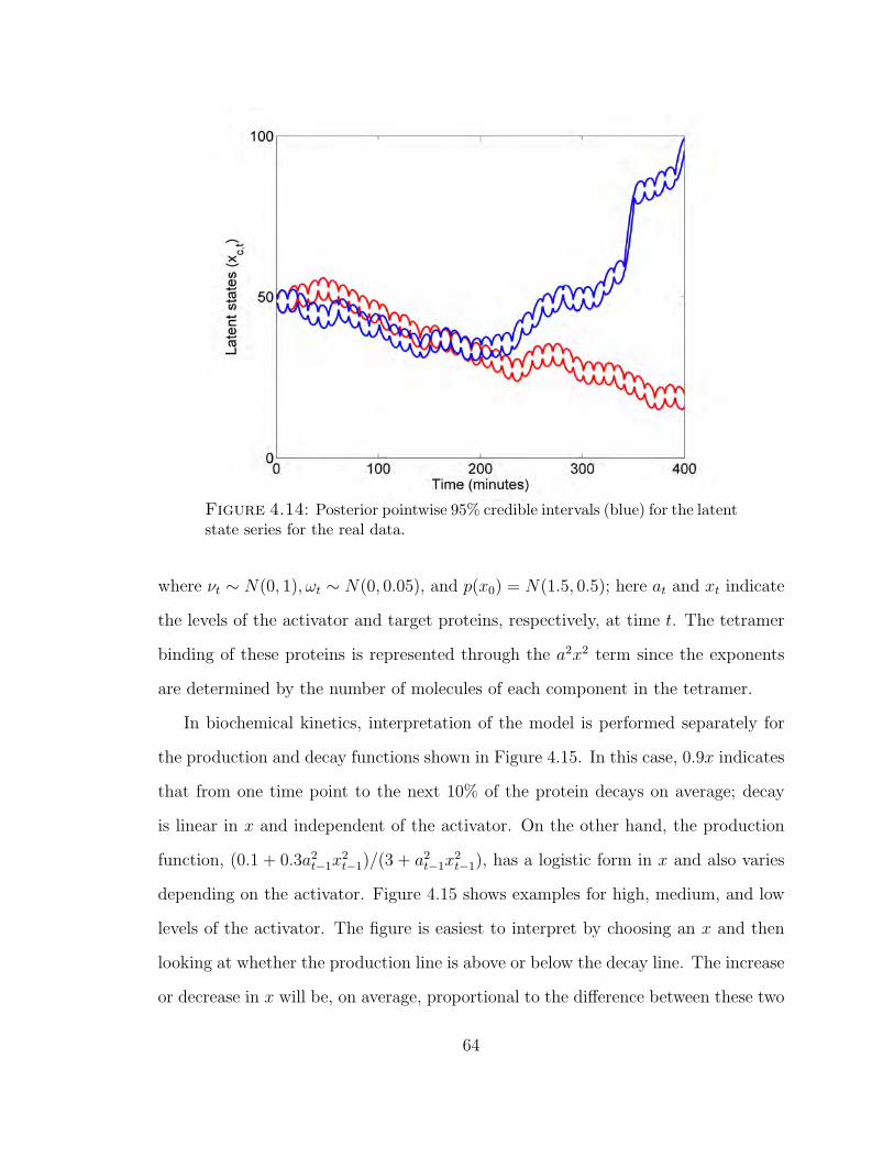
Figure 4.14: Posterior pointwise 95% credible intervals (blue) for the latentstate series for the real data.
where νt ∼ N(0, 1), ωt ∼ N(0, 0.05), and p(x0) = N(1.5, 0.5); here at and xt indicate
the levels of the activator and target proteins, respectively, at time t. The tetramer
binding of these proteins is represented through the a2x2 term since the exponents
are determined by the number of molecules of each component in the tetramer.
In biochemical kinetics, interpretation of the model is performed separately for
the production and decay functions shown in Figure 4.15. In this case, 0.9x indicates
that from one time point to the next 10% of the protein decays on average; decay
is linear in x and independent of the activator. On the other hand, the production
function, (0.1 + 0.3a2t−1x
2t−1)/(3 + a2
t−1x2t−1), has a logistic form in x and also varies
depending on the activator. Figure 4.15 shows examples for high, medium, and low
levels of the activator. The figure is easiest to interpret by choosing an x and then
looking at whether the production line is above or below the decay line. The increase
or decrease in x will be, on average, proportional to the difference between these two
64

lines.
In reality, the activator often has an oscillating pattern – related to the progression
through cell cycles – and scientists are interested in the response of the target. Figure
4.16 shows the level of the oscillating activator and the observations for a simulated
data set with T = 180. Inference on xt levels is important since the target protein
may affect genes downstream in the overall biological pathway. From the data in
this plot, it seems clear that periodicity exists; however, due to the realistically high
degree of measurement noise, it is unclear what exactly the levels of the underlying
protein are. This can be particularly important when downstream target genes are
extremely sensitive to the levels of the protein, perhaps only being expressed when
the protein passes a certain threshold.
AM4 was applied using J = 100, again saving 100,000 MCMC samples after the
same length burn-in and now achieving a Metropolis acceptance rate of 41%. Figure
4.17 provides a graphical summary of the inferred trajectory of the target protein
in terms of pointwise median and 95% credible interval for each p(xt|y1:T ) from the
MCMC output. The known “true” target values are overlaid. For reference, the
activator is included showing how the target response oscillates in a delayed fashion
relative to the activator.
4.6.1 Multivariate states and parameters
Scientists are naturally interested in models with state vectors in more than one
dimension, and have studied a number of examples with analysis based on the im-
mediate application of the above computational strategy now extended via a Gibbs
sampling set to treat each of the individual states. The alternative approach –
extending the general mixture strategy to be based on multivariate mixtures – is
certainly of interest but beyond the scope here, while the coupling of univariate sam-
plers within a Gibbs framework is immediate and, in these examples, effective. As
65

Figure 4.15: Model of (4.6): Production and decay functions for variouslevels of the activator.
Figure 4.16: Model of (4.6): The upper plot shows the known level ofactivator and the lower plot shows the observation at all time points.
66

Figure 4.17: Model of (4.6): Pointwise median (solid, blue) and 95%credible interval (dotted, blue) results for the target protein (black). Theactivator (red) is shown for reference.
an example, I examine the above model now including inference on both activator
and target state variables.
The more realistic version of the above model in equations (4.6) involves measure-
ments on both the activator and the target protein as well as uncertainty about the
parameters in the evolution functions. As an example, suppose that the evolution
function for the activator is an autoregressive process whose mean varies depending
on the on/off state of the activator that is controlled experimentally. The full model
is then
yt =
(atxt
)+ νt
(atxt
)=
(µct + φ(at−1 − µct)
(k + αa2t−1x
2t−1)/(β + a2
t−1x2t−1) + ψxt−1
)+ ωt
(4.7)
where ct ∈ 0,1, νt ∼ N(0, σ2mI), and ωt ∼ N (0, diag(σ2
a, σ2x)) again independent
67

and mutually independent. Simulations were performed up to T = 180 using k =
0.01, α = 0.3, β = 4, ψ = 0.9, µ0 = 0.5, µ1 = 2.5, φ = 0.9, σm = 1, σa = 0.05,
σx = 0.05, x0 = 1.5 and a0 = 1.5 and the results are shown in Figure 4.19.
Informative priors are used for all fixed parameters either to truncate the parame-
ters to reasonable regions or to provide information on plausible biological knowledge.
For example, many parameters are products of chemical kinetic reaction parameters.
Since chemical kinetic parameters are all positive, their products are also positive.
This includes the parameters k, α, β, µ0, and µ1 which are given positive Gaussian
distributions with expected value equal to the truth and scales (standard deviations)
of 0.032, 1, 1, 0.1, and 0.1, respectively. The autoregressive parameters, i.e. the
percentage of protein remaining from the previous time point, are given Gaussian
priors truncated to the interval (0,1). Both priors have expected value equal to the
truth and scales of 0.1 which are fairly diffuse. Finally, priors for the variance terms
are given scaled inverse χ2 with degrees of freedom of 3 and expected values equal
to the truth.
The analysis performed through MCMC is decomposed into Gibbs and Metropolis
steps. The steps are all univariate with the exception of the draws for the latent states
of the activator a0:T and the target x0:T . All fixed parameters with the exception of
β are available as Gibbs steps and a random walk Metropolis was used for β. The
joint draw for a0:T is available using FFBS neglecting the evolution equation for x
and then using this as a Metropolis proposal. The joint draw for x0:T is performed
through AM4 of Chapter 2. More details on the full conditional distributions for all
model parameters is provided in Appendix C.2.
The full MCMC analysis was performed using J = 10 mixture components for
the target protein Metropolis step, saving 50,000 iterations after 5,000 burn-in, and
achieving a Metropolis acceptance probabilities of 40%, 43%, and 9% for β, x0:T , and
a0:T respectively. Figure 4.18 provides the posterior marginal histograms for fixed
68

Figure 4.18: Model of (4.7): Histograms of marginal posterior estimates(blue), prior (green), and true value (red) for fixed model parameters.
model parameters as well as the priors and true values used in the simulation. This
figure shows that little information is gained about k, µ0, and µ1. On the other
hand, α, ψ, φ, and σm all have more informed posteriors relative to their priors. In
contrast, although the priors were meant to be uninformative for parameters β, σx,
and σa very little information is gained in the analysis.
Figure 4.19 provides posterior median and pointwise 95% credible intervals for
the activator and target protein. The credible intervals appear to capture the truth
quite accurately and these inferences are much more accurate than the observed data.
As mentioned earlier, these plots would be particularly useful when combined with a
larger model where the target protein affected downstream proteins via a threshold
69

Figure 4.19: Model of (4.7): Pointwise median (solid) and 95% credibleinterval (black) results for the underlying state (red) for the activator (top)and target (bottom) proteins.
or similar method since MCMC methods allow for calculating the probability of the
target protein being above or below that threshold at each time point.
4.6.2 Mis-specified prior for nonlinear parameter
As mentioned previously, little scientific knowledge is available for the nonlinear
parameter β. In this section, I intentionally mis-specify the parameter β by giving
it a prior with expected value 12 and standard deviation of 1 when the true value is
3. I then analyze how this mis-specification affects the inference on β and all other
parameters.
Exactly the same settings are used for this analysis as were used in the previous
with the exception of this parameter. Figure 4.20 provides posterior histograms for
fixed model parameters when the prior on β is mis-specified. Most of the parameters
appear unaffected by this mis-specified prior. The posterior for β appears to be,
70

Figure 4.20: Model of (4.7): Histograms of marginal posterior estimates(blue), prior (green), and true value (red) for fixed model parameters whenthe prior for β is inaccurate.
if anything, moving toward the true value relative to the prior, but this change is
certainly slight. The only other parameter that appears to be affected is ψ, the
percentage of target protein remaining from the previous step. This should come
as no surprise since β reduces the production of the target protein and therefore ψ
compensates by increasing the amount of target protein retained from the previous
time point. Results for the latent states are not shown as there was very little
difference from the previous analysis.
4.6.3 Inference on unmeasured components
One question that arises in the analysis of systems biology models is that of inference
on components of the system for which no measurements are taken. The biological
models that are described here are founded on the underlying levels of DNA, RNA,
and other proteins that are not specifically modeled; see Appendix A. A natural
71

question is: what information can be obtained about unmeasured components in the
system?
I begin with the system described in equations (4.7). In the previous section, all
fixed parameters are assumed unknown, although some had informative priors, and
both of the components of interest were observed with noise. In this section, I assume
no observations are taken on the activator and try to understand what information
can be obtained concerning its level.
In the following two subsections, I analyze this question making two different
assumptions. In Section 4.6.4, inference is performed for the latent activator level
when all fixed parameters and the level of the target protein are known. In Section
4.6.5, I relax the assumption of all known parameters by relaxing the priors in the
evolution equation for the activator.
4.6.4 All fixed parameters and target level known
Earlier, I performed an analysis of a simulated systems biology example containing
an activator and a target protein and their underlying dynamics. The evolution
and observation equations contained 10 fixed parameters that were inferred from the
measured levels of the two proteins. Here I assume that all fixed parameters and
the target protein level are known, but no measurements are taken on the activator.
The objective is to understand how much information is available about the latent
state of that activator.
Figure 4.21 shows the prior and posterior for the latent activator level when the
stationary means, autoregressive parameter, and evolution variance for the activator
are all known, but no measurements are taken on the activator. From this figure,
it is clear that the prior itself is very informative about the level of the activator.
Recalling equations (4.7), the posterior shows the additional information provided
on the activator by the evolution equation for the target protein. The most obvious
72

Figure 4.21: Pointwise 95% credible intervals (dashed) and median (solid)for the prior (gray) and the posterior (black) for latent activator protein levelwhen no measurements are taken on this protein and all fixed parameters areknown.
difference occurs initially where the credible interval is much tighter for the posterior
than for the prior. In addition, differences can be seen as shifts in the troughs where
in the first trough the posterior is shifted higher and in the second and third the
posterior is shifted lower.
4.6.5 Relaxing priors on fixed parameters
I now relax the assumption of all fixed parameters known by allowing the variance
for the activator evolution to be unknown. This parameter is given diffuse scaled
inverse χ2 distribution with degrees of freedom of 3 and scale of 0.052/3 so that
the expected value is the truth. All other parameters are assumed known at their
true values including the target protein level. So although the stationary means and
autoregressive parameter are known, both the marginal and conditional distributions
for the activator have unknown variance.
Figure 4.22 displays the prior and posterior for the activator level when the evo-
lution variance is known but no measurements are taken on the activator. This
figure shows that the pointwise 95% credible intervals are slightly wider for the prior
73
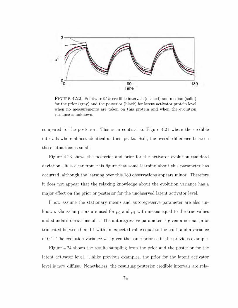
Figure 4.22: Pointwise 95% credible intervals (dashed) and median (solid)for the prior (gray) and the posterior (black) for latent activator protein levelwhen no measurements are taken on this protein and when the evolutionvariance is unknown.
compared to the posterior. This is in contrast to Figure 4.21 where the credible
intervals where almost identical at their peaks. Still, the overall difference between
these situations is small.
Figure 4.23 shows the posterior and prior for the activator evolution standard
deviation. It is clear from this figure that some learning about this parameter has
occurred, although the learning over this 180 observations appears minor. Therefore
it does not appear that the relaxing knowledge about the evolution variance has a
major effect on the prior or posterior for the unobserved latent activator level.
I now assume the stationary means and autoregressive parameter are also un-
known. Gaussian priors are used for µ0 and µ1 with means equal to the true values
and standard deviations of 1. The autoregressive parameter is given a normal prior
truncated between 0 and 1 with an expected value equal to the truth and a variance
of 0.1. The evolution variance was given the same prior as in the previous example.
Figure 4.24 shows the results sampling from the prior and the posterior for the
latent activator level. Unlike previous examples, the prior for the latent activator
level is now diffuse. Nonetheless, the resulting posterior credible intervals are rela-
74

Figure 4.23: Posterior histogram and prior (green) for the evolution stan-dard deviation of the activator.
Figure 4.24: Pointwise 95% credible intervals (dashed) and median (solid)for the prior (gray) and the posterior (black) for latent activator protein levelwhen no measurements are taken on this protein and all evolution parametersare unknown.
75

Figure 4.25: Posterior histogram and prior (green) for activator evolutionparameters. Clockwise from top left the parameters are µ0, µ1, φ, and σa.
tively tight. A couple of apparent artifacts can be seen, but these were consistent
across multiple runs of the MCMC. Since the information about the activator level is
coming through the evolution equation for the target, presumably these “artifacts”
reflect an extreme target protein level. This analysis suggests that a lot of infor-
mation about the activator is passed through the evolution equation for the target
protein.
We can also evaluate the learning about the activator evolution parameters by
their posteriors in Figure 4.25. The stationary means and autoregressive parameter
have posteriors very distinct from their priors whereas the evolution standard devi-
ation is approximately the same. A progression of increasing knowledge can be seen
76

which impacts parameter estimates and, in turn, the latent activator state. With lit-
tle knowledge of parameters, i.e. the prior in Figure 4.24, the intervals for the latent
activator state are large. As knowledge about the fixed parameters increases, e.g.
the posterior in Figure 4.24, our uncertainty about the activator decreases. When
knowledge about these parameters is complete, e.g. Figure 4.21, the intervals for the
latent activator are the most precise.
4.7 Summary
This chapter explored some discrete time models for biological systems and MCMC
analyses on simulations and real data. The objective was to estimate parameters and
unknown states while understanding the affect of knowledge about different model
components. Beginning from a mechanistic approach outlined in Appendix A, it is
clear that many chemical kinetic parameters in the system will never be identified
solely by the data. Even aggregating these parameters to build a dynamic model
requires the use of informative priors with data of the sort analyzed here.
Experiments will need to be carefully designed to isolate model parameters and
allow for their identification by data. In particular, some suggestions for possible
future experiments are listed here.
• Take repeated measurements of the system to understand the observation vari-
ance.
• At each time point, activate fluorescent proteins with a small amount of exci-
tation light and take a measurement. Repeat this multiple times at that time
point to understand the relationship between protein amount and observed
fluorescence.
• Build a system with a highly stable protein and no production of that protein
77

and little bacterial growth. Measure this protein repeated through time to
understand the measurement error variance.
• Build a system that can be initiated with high protein concentration and such
that the no more protein is produced to isolate the decay parameter.
• Build a system where the protein can be maintained at a high level, i.e. no cell
growth, to estimate the high-protein production rate.
• Build a system where the protein can be maintained at a low level by, for
example, washing away a protein that can easily permeate the cell membrane.
This will isolate the low production rate.
The understanding of in vitro systems will be enhanced when we are able to
decompose the system into components that can be studied in isolation. This will
facilitate model building, parameter estimation, and use of previous experiments as
priors for future models.
78

5
Nonlinear, non-Gaussian models: an example inhistorical analysis of US dollar - British pound
exchange Rate
The previous chapters have discussed the case of nonlinear but Gaussian models.
This chapter aims to extend that discussion to general dynamic models. In the
nonlinear examples, the observation and evolution functions were linearized using a
first-order Taylor series expansions which kept the Gaussian error structure intact. In
general dynamic models, this linearization is not applicable. The approach here is to
update the mixture components approximately by taking a Gaussian approximation
of the density around each mixture component. As a motivating example, I look at
stochastic volatility models and data on the US Dollar - British pound exchange rate
over several years.
5.1 Analysis of stochastic volatility models
The efficient fitting of models with stochastic volatility is a challenge in modern time
series analysis (Taylor, 1986; Jacquier et al., 1994). These models can be interpreted
79

as dynamic models where the unobserved states determine the variability in the
observation equation. These models arise out of a generalization of the Black-Scholes
option pricing equation by allowing the variance to change over time (Hull and White,
1987; Chesney and Scott, 1989; Melino and Turnbull, 1990; De Jong and Shephard,
1995).
The simplest stochastic volatility model has the form
rt = σtνt, (5.1a)
log σt = µ+ φ(log σt − µ) +√Wωt, (5.1b)
where νt and ωt are standard normals that are independent across time and mu-
tually independent. The observations, rt, are daily (or weekly) returns on an in-
vestment of interest, σt is the volatility, and the fixed parameter is three dimen-
sional: θ = µ, φ,W. Extensions of this model include regression terms, e.g.
rt ∼ N(x′tβ, σ2t ), or heavy-tailed distributions (Chib et al., 2002; Jacquier et al.,
2004). Slight modifications of the methods developed in this chapter apply to these
cases.
The likelihood function, i.e. f(θ) ∝ p(r1:T |θ) for a fixed set of returns r1:T , in these
stochastic volatility models is hard to evaluate and, for this reason, early statistical
analyses have avoided this computation. Taylor (1986), Melino and Turnbull (1990),
and Vetzal (1992) used method of moments to avoid the integration involved with
the likelihood computation. Nelson (1988), Harvey et al. (1994), and Ruiz (1994)
developed a quasi-maximum likelihood estimator by approximate linear filtering.
Danielsson and Richard (1993) and Danielsson (1994) develop a simulation approach
to deriving maximum likelihood estimates termed accelerated Gaussian importance
sampler.
In contrast to these approaches, Bayesian techniques perform the integration
using sampling methods such as MCMC. These methodologies draw samples from
80

Table 5.1: Component probabilities (pj), means (ηj), and variances (ς2j ) for
a mixture of normals to approximate the distribution of a log(χ21)/2 random
variable.pj : 0.00730 0.00002 0.10556 0.25750 0.34001 0.24566 0.04395ηj : −5.7002 −4.9186 −2.6216 −1.1793 −0.3255 0.2624 0.7537ς2j : 1.4490 1.2949 0.6534 0.3157 0.1600 0.0851 0.0418
p(θ, σ1:t|r1:t) by alternating draws from p(θ|σ1:t, r1:t) and p(σ1:t|θ, r1:t). In addition,
some of these methods further decompose the state draw into a sequence of draws
from each marginal distribution, i.e. p(σj|σ−j, θ, r1:t). For example, Carlin et al.
(1992) were the first to suggest this general approach in dynamic models where they
used accept/reject methods within a Gibbs sampling context. Improvements upon
this general methodology in stochastic volatility models include Jacquier et al. (1994)
who utilize accept/reject methods where practical and augment with Metropolis steps
when necessary.
In contrast to these MCMC approaches which sample from individual states at
a time, Carter and Kohn (1994) and Shephard (1994) suggest sampling from the
full joint distribution of all states simultaneously. Their suggestion is based on the
linearization of equation (5.1a) such that yt = log(r2t )/2. Then yt = xt + ηt where
xt = log σt, ηt = log(κt)/2, and κt ∼ χ21. They then approximate the distribution
for ηt by a mixture of normals which was implemented in Kim et al. (1998). Table
5.1 provides the component probabilities, means, and variances for a 7-component
mixture of normals approximation to the log(χ21)/2 distribution. Figure 5.1 presents
a graphical illustration showing the good approximation found in the main mass of
the distribution and the errors in approximating the left tail.
The MCMC is then augmented with an auxiliary variable at each time point,
λt ∈ 1, 2, . . . , 7. These auxiliary variables indicate which mixture component each
observation is drawn from. This MCMC scheme draws samples from the joint distri-
bution p(θ, x1:t, λ1:t|y1:t) which has the target distribution p(θ, x1:t|y1:t) as a marginal.
81

Figure 5.1: Density of a log(χ21)/2 random variable (green) and a 7-
component mixture of Gaussians approximation (blue) with the 7 com-ponents (red). Left plot shows the left tail while the right plot showsthe main mass of the distribution.
The additional task of sampling from p(λ1:t|θ, x1:t, y1:t) can be done component-wise
due to conditional independence of λt across time. The benefit of this approach is
that the full conditional distribution for the volatility state process can be sampled
jointly using FFBS.
5.2 Non-Gaussian mixture updating
Similar to the approach of Kim et al. (1998), I aim to sample the distribution for the
latent states jointly conditional on the fixed parameters. The steps in this procedure
are similar to those outlined in Section 2.1. I use the notation xt = log σt, where xt is
an autoregressive process according to equation (5.1b). Assuming that the posterior
for the state at time t− 1, namely p(xt−1|y1:t−1), is a mixture of Gaussians, the first
step is to propagate this distribution through the evolution equation to obtain the
prior for the state at time t. Since the evolution equation in a stochastic volatility
model is linear and Gaussian, the prior is trivially a mixture of Gaussians. I update
this mixture according to the observed value yt and the observation equation p(yt|xt).
In this stochastic volatility example, the observation equation is given by yt = xt+ηt
82

Table 5.2: Equations for approximately updating a normal mixturex ∼ Nm(p1:J , a1:J , R1:J) given an observation y from an arbitrary ob-servation density p(y|x). These equations provide the approximate pos-terior p(x|y) = Nm(p′1:J ,m1:J , C1:J). The notation d1(a) and d2(a) in-dicate the first and second derivatives of x of the logarithm of the ob-servation density evaluated at a, respectively. See Appendix B for fulldetails.
p′j ∝ pjp(y|aj)N
(d1(aj)
d2(aj)
∣∣∣ 0, d2(aj)−1 +Rj
)N
(d1(aj)
d2(aj)
∣∣∣ 0, d2(aj)−1)
mj = Cj
(d2(aj)
[aj −
d1(aj)
d2(aj)
]+ aj/Rj
)Cj = (d2(aj) + 1/Rj)
−1
where each ηt is an independent log(χ21)/2 random variable. This mixture will provide
a posterior for the latent state at time t that is a mixture of Gaussians.
In order to update a mixture of Gaussians given an arbitrary observation equa-
tion, we approximate the observation density using a second-order Taylor series ex-
pansion of the logarithm of that density around the expected value of each mixture
component. This approximation provides a mixture of Gaussians which can be up-
dated for each mixture component individually and then the component probabilities
can be updated according to the predictive distribution for each component. Given a
prior for x that is a mixture of Gaussians, i.e. x ∼ Nm(p1:J , a1:J , R1:J), the posterior
is then approximately given by x|y ∼ Nm(p′1:j,m1:j, C1:j) where the updating rules
are given in Table 5.2 with details and code provided in Appendices B and D.5,
respectively. The intuition here is that the observation density is approximated by
a Gaussian with precision d2(a) and mean d1(a)/d2(a) where a is the Taylor series
expansion point and d1 and d2 are the first and second derivatives of the logarithm
of the observation density, respectively. Each component is updated according to
its own mean aj and the component probabilities are updating according to the
83

Table 5.3: Equations for approximately updating a normal mixture x ∼Nm(p1:J , a1:J , R1:J) given an observation y from the model y = x + ηwhere η is a log(χ2
1)/2 random variable. Plugging these values into theequations in Table 5.2 complete the updating.
p(y|aj) = (π/2)−1/2 exp(y − aj − e2(y−aj)/2
)d1(aj) = 1− e2(y−aj)
d2(aj) = 2e2(y−aj)
predictive distribution for each component.
5.2.1 Updating filtered distributions in a stochastic volatility model
In this stochastic volatility example, the filtered distribution for the state at time t−1
is approximated by a mixture of Gaussians. This implies a prior for the state at time
t that is a mixture of Gaussians due to the linear Gaussian nature of the evolution
equation. Using Tables 5.2 and 5.3 together, this prior can be approximately updated
given an observation yt = log(r2t )/2.
If iterated, this procedure provides a means to obtain the filtered distributions
for the latent states given a sequence of observations. Similar to the situation in non-
linear Gaussian models, this procedure can cause degeneration in the mixture com-
ponents. In order to combat this degeneracy, the regeneration procedure discussed
in Table 2.1 is used after each updating step. This procedure sets the component
probabilities equal, the component means to be the quantiles of the distribution,
and the variances equal such that the overall variance matches that of the true dis-
tribution. Figure 5.2 shows the effect of this regeneration procedure as well as the
resulting posteriors. The prior for x in this figure was produced using a randomly
generated 5-component mixture of normals. It is clear that as the number of mixture
components is increased the approximation to the posterior is more accurate. Also,
the the posterior under all of the regenerated distributions is more diffuse than the
84

Figure 5.2: Prior (left) and posterior (right) for x under a randomlychosen prior and the observation model y = x+ ν where ν ∼ log(χ2
1)/2.Shown are approximations to the truth (black) based on the regenerationprocedure of Section 2.2.4 using 2 (red), 10 (green), and 100 (blue)mixture components.
truth which is beneficial as a Metropolis proposal.
To build AM4 for the stochastic volatility model, I incorporate the use of the
regeneration procedure. Since the evolution equation is linear Gaussian, the prop-
agation of the mixture of Gaussians from posterior at time t − 1 to prior at t is
exact and therefore no regeneration is necessary. The regeneration procedure is used
once per filtering iteration after the prior has been updated using Table 5.2. One
iteration of the adaptive mixture filtering procedure for stochastic volatility models
is provided in Table 5.4 and code is provided in Appendix D.6.
5.2.2 Metropolis-Hastings sampling of the volatility
The procedure as outlined provides approximations to the filtered distributions for
the state at all time points based on a mixture of Gaussians at each time point.
In order to obtain a sample from the joint distribution for all latent states, we use
the backward sampling procedure outlined in Chapter 2. This procedure draws an
approximate sample from the joint posterior for all latent states. In order to obtain
a true draw, this proposed sample is corrected using a Metropolis-Hastings step as
85

Table 5.4: Algorithm for adaptive mixture filtering in the stochastic volatilitymodel shown in equations 5.1.
1. Assume we have p(xt−1|y1:t−1).
2. Use RP1 on p(xt−1|y1:t−1) to obtain Nm(pt−1,1:J ,mt−1,1:J , Ct−1,1:J).
3. Calculate the one-step ahead prior
p(xt|y1:t−1) = Nm(pt−1,1:J , at−1,1:J , Rt−1,1:J)
where
at,j = µ+ φ(mt−1,j − µ) and Rt,j = φ2Ct−1,j +W.
4. Update the mixture components based on the observed data yt =log(r2
t )/2 to obtain p(xt|y1:t) = Nm(p′t,1:J , mt,1:J , Ct,1:J) accordingto the equations in Tables 5.2 and 5.3.
outlined in Section 2.3. We then accept or reject this sample accordingly and, in the
limit, have a draw from the stationary distribution of the Markov chain, namely the
target distribution p(x0:t|y1:t).
5.3 MCMC algorithm for stochastic volatility example
In a running theme, the full MCMC for this stochastic volatility example involves
alternating draws from parameters given states followed by states given parameters.
The previous section outlined the procedure for sampling from the states given the
parameters. One piece of information omitted from the previous section was the
prior for the initial state. In order to ensure stationarity of the model, we assume the
initial prior is x0 ∼ N(µ,W/(1− φ2)). In sampling for the states given parameters,
this simply means approximating this prior by a mixture of Gaussians using the
regenerating procedure and then adjusting for this approximation in the Metropolis
acceptance probability.
The full parameter vector is θ = µ, φ,W and sampling is performed on each
86
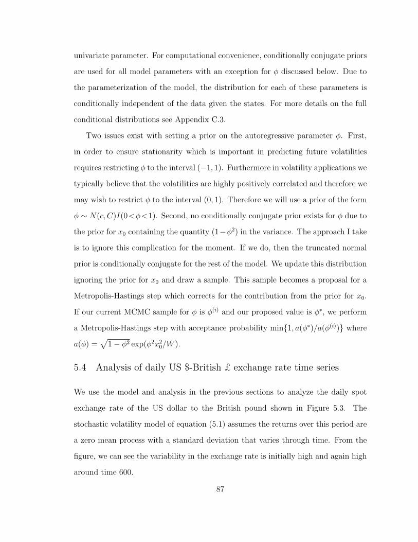
univariate parameter. For computational convenience, conditionally conjugate priors
are used for all model parameters with an exception for φ discussed below. Due to
the parameterization of the model, the distribution for each of these parameters is
conditionally independent of the data given the states. For more details on the full
conditional distributions see Appendix C.3.
Two issues exist with setting a prior on the autoregressive parameter φ. First,
in order to ensure stationarity which is important in predicting future volatilities
requires restricting φ to the interval (−1, 1). Furthermore in volatility applications we
typically believe that the volatilities are highly positively correlated and therefore we
may wish to restrict φ to the interval (0, 1). Therefore we will use a prior of the form
φ ∼ N(c, C)I(0<φ<1). Second, no conditionally conjugate prior exists for φ due to
the prior for x0 containing the quantity (1−φ2) in the variance. The approach I take
is to ignore this complication for the moment. If we do, then the truncated normal
prior is conditionally conjugate for the rest of the model. We update this distribution
ignoring the prior for x0 and draw a sample. This sample becomes a proposal for a
Metropolis-Hastings step which corrects for the contribution from the prior for x0.
If our current MCMC sample for φ is φ(i) and our proposed value is φ∗, we perform
a Metropolis-Hastings step with acceptance probability min1, a(φ∗)/a(φ(i)) where
a(φ) =√
1− φ2 exp(φ2x20/W ).
5.4 Analysis of daily US $-British £ exchange rate time series
We use the model and analysis in the previous sections to analyze the daily spot
exchange rate of the US dollar to the British pound shown in Figure 5.3. The
stochastic volatility model of equation (5.1) assumes the returns over this period are
a zero mean process with a standard deviation that varies through time. From the
figure, we can see the variability in the exchange rate is initially high and again high
around time 600.
87

Figure 5.3: Changes in the daily spot exchange rate of the US dollarto the British pound over a period of 1000 days ending on 8/9/96.
5.4.1 Informative prior for evolution variance
The first analysis of this data places an informative prior on the evolution variance
W , namely a scaled inverse chi-squared distribution with degrees of freedom 1000
and scale parameter 0.01. Since the posterior will provide another 1000 degrees of
freedom, this prior places equal weight on the data and the prior. The priors for the
stationary mean and autoregressive parameter are diffuse and Gaussian, although
the autoregressive parameter is truncated between 0 and 1 to ensure a stationary
and a positively correlated series.
I compare our approach to the approach of Kim et al. (1998), referred to as KSC,
who approximate the additive log(χ21)/2 distribution by a mixture of Gaussians. The
KSC analysis implemented here utilizes a different prior and sampling scheme for φ,
but otherwise remains the same. The sampling steps for all fixed parameters under
88

these two sampling schemes are identical. The difference is in the sampling of the
latent states. In the method described in this chapter, I use AM4 as described
above with J = 10 components to provide a Metropolis proposal draw. In contrast,
KSC samples states using two steps in the MCMC. The first step involves sampling
mixture indicators for each time point and the second involves an FFBS step for joint
sampling of the entire state vector conditional on these indicators. The stationary
distributions for these two chains are different; the stationary distribution for KSC
is an approximation to the true model, whereas our approach has the exact posterior
as the stationary distribution.
Figure 5.4 provides posterior histograms under the two different sampling schemes.
The two approaches are relatively close, but the evolution standard deviation appears
larger while the autoregressive parameter and mean are slightly smaller under KSC.
Figure 5.5 compares the pointwise 95% credible intervals and means for the latent
volatility under the two models. In general, AM4 has narrower credible intervals.
Nonetheless, these two analyses seem to provide fairly comparable results.
5.4.2 Uninformative prior for evolution variance
In the previous analysis, the evolution variance was given a fairly informative prior.
In particular, the weight of the prior was, in some sense, equal to the weight given by
the data. In the next analysis, I reduce the weight given to the prior by adjusting the
degrees of freedom in the inverse chi-squared distribution down to 10 and keeping
the same scale parameter.
Figure 5.6 provides posterior histograms under the two analyses using this less
informative prior. These results are much more disparate than the previous results.
The stationary mean is about equal in the two models. The evolution standard
deviation is approximately 10 times as large using the approximate model. The
autoregressive parameter is around 0.95 using our method and is around 0.1 using
89

Figure 5.4: Posterior histograms and priors (green) for stochasticvolatility model parameters using AM4 (blue) and KSC (red) when theevolution standard deviation is given an informative prior.
Figure 5.5: Pointwise 95% credible intervals for the volatility (σt)using AM4 (blue) and KSC (red) where
√W is given an informative
prior.
90

Figure 5.6: Posterior histograms and priors (green) for stochasticvolatility model parameters using AM4 (blue) and KSC (red) when theevolution standard deviation is given a relatively uninformative prior.
Figure 5.7: Pointwise 95% credible intervals for the volatility (σt)using AM4 (blue) and KSC (red) where
√W is given a relatively unin-
formative prior.
91

the approximate model. These differences are magnified in the estimation of the
volatility shown in Figure 5.7. The credible intervals for the approximate model are
much wider and there is less agreement from day to day. This is consistent with
the parameters in this model which show that the volatility from day to day is only
slightly correlated and the evolution variance is large. Therefore, given the posteriors
for the fixed parameters, it is not surprising to observe the differences in volatility.
Nonetheless, the differences between these two methods in this analysis is striking.
This difference is presumably due to the inadequacies of the mixture approxima-
tion to the log(χ21)/2 distribution in the left tail. The approximate model cannot
account for large negative returns simply due to the observation equation. In order
to account for these large negative returns, the approximate model must account for
these observations using the latent volatility. The latent volatility must be allowed to
be very high at that time point. Since observations around this extreme observation
are not necessarily extreme themselves, the latent volatility will be small at sur-
rounding time points. This lack of autocorrelation and large variations in volatility
are supported by the posteriors for φ and√W .
5.5 Summary
This chapter developed a method for using AM4 on nonlinear and non-Gaussian mod-
els. The idea rests upon updating Gaussian mixture components by approximating
non-Gaussian distributions locally by Gaussians. This provides a proposal for the
joint distribution of the vector of latent states that is accepted using a Metropolis-
Hastings step. I implemented this approach in a stochastic volatility example ana-
lyzing US $ - British £ exchange rate data.
This analysis showed comparable results with an approximate model based on
approximating the log(χ2)/2 error in the observation by a mixture of Gaussians when
an informative prior is used on the evolution variance. The same cannot be said for
92

an uninformative prior on the evolution variance where the two analyses differed
dramatically. The only difference between the two analyses was the sampling of the
latent states. The approximate model jointly samples the latent states using FFBS
conditional on mixture component indicators and then samples the indicators as part
of the MCMC.
This analysis suggests that the deficiency in the mixture of Gaussians approxi-
mation to the log(χ2)/2 density provides inaccurate inferences about the true model
parameters in equations 5.1. Expanding the approximation beyond a 7-component
mixture should reduce the inaccuracies but not eliminate them. These inaccuracies
can be overcome by enforcing a slow moving volatility process through an informative
prior on the evolution variance.
93

6
Sequential Monte Carlo methods
The analysis of the previous chapters has focused on analysis of time series data
in batch. Often time series data is available sequentially and therefore data should
be processed as it arrives. This is often accomplished using particle filtering meth-
ods, such as sequential importance sampling, where a weighted sampled from the
filtered distribution at one time point is used to generate a weighted sample for the
filtered distribution at the following time point. Breakthroughs came with Gordon
et al. (1993) and West (1993b) where the authors fought against state degeneracy
by incorporating resampling and local smoothing at each step in the iterative pro-
cedure. Further improvements of these approaches are available, including notably
the auxiliary particle filter (APF) in Pitt and Shephard (1999).
These widely used algorithms often perform well when all fixed parameters are
known, but suffer from degeneracy issues when parameters are unknown. A naive
approach incorporates unknown fixed parameters into the state vector. These new
‘states’ have no evolution since they are fixed. Unfortunately, the resampling step
necessary to avoid dynamic state degeneracy induces attrition in the set of particles
representing fixed parameters. This occurs because samples for fixed parameters
94

are only drawn at the initial time point. An initial approach, first suggested in
Gordon et al. (1993) using the term roughening penalty and, at the same time and
independently, in West (1993b) using local kernel smoothing of particles, is to add
artificial evolution noise to the parameters. This allows a whole new set of parameter
values at each step in the procedure. As pointed out in West (1993b), and in more
detail in Liu and West (2001), one serious drawback of this approach is that the
parameters are fixed and introducing artificial noise induces a loss of information
about these parameters.
A reconciliation of this problem is provided in Liu and West (2001) who use the
kernel smoothing ideas (West, 1993a) to regenerate fixed parameters at each step in
their algorithm. The roughening penalty is essentially derived from a kernel density
estimate of currently sampled parameter values and this estimate is over-dispersed
relative to the samples. In order to correct for this over-dispersion, kernel shrinkage
ideas can more accurately approximate the mean and variance-covariance matrix
implied by the parameter samples. This framework provides a easily implemented
algorithm that can be used in arbitrary dynamic models. Unfortunately, as will be
shown in Section 6.2.3, this approach sometimes reduces the degeneracy only slightly
and new methods are still needed to further combat degeneracy.
A different approach to dealing with degeneracy in parameters utilizes sufficient
statistics. Introduced in Storvik (2002) and Fearnhead (2002) and further developed
in Carvalho et al. (2008), these sufficient statistic ideas suggest an approach where
particles carry sufficient statistics for parameters rather than samples of parameters
themselves. Inference for parameters can then be performed off-line using the dis-
tribution for the parameters conditional on the sufficient statistics. As will be seen
in Section 6.2.3, these methods can reduce degeneracy dramatically. Unfortunately
the model class for which they can be used is limited.
To expand the model class for which sufficient statistics can be used, I partition
95

the fixed parameters into two subsets. One of these subsets has no convenient suf-
ficient statistic structure, but the other, conditional on the first, does. I then use
the kernel smoothing approach of Liu and West (2001) to update the first set of
parameters and then sufficient statistics for the second set. This allows for the re-
duced degeneracy that the sufficient statistics provide while being broadly applicable
to a large model class. The chapter is organized as follows. Section 6.2 describes
the kernel smoothing and sufficient statistic ideas in detail. Section 6.2.3 compares
these two approaches in terms of degeneracy in fixed parameters and computation
time. Section 6.3 introduces the algorithm for combining the kernel smoothing and
sufficient statistic ideas and Section 6.4 provides an example.
6.1 Sequential Monte Carlo with known parameters
Consider the general dynamic model defined by equations (6.1) with initial state
distribution p(x0|θ),yt ∼ p(yt|xt, θ), (observation equation) (6.1a)
xt ∼ p(xt|xt−1, θ). (evoution equation) (6.1b)
I first consider the fixed parameters θ as known and therefore suppress them in
notation for the remainder of this section. The aim here is to sequentially estimate
the posterior distribution at time t, namely p(x0:t|y1:t), including as a marginal the
filtering distribution p(xt|y1:t) and other features.
At any time t, this posterior distribution is given by Bayes’ theorem
p(x0:t|y1:t) ∝p(y1:t|x0:t)p(x0)∫p(y1:t|x0:t)p(x0)dx0:t
.
A recursive formula for sequentially determining the posterior distribution at the
next time point is available via the relationship
p(x0:t+1|y1:t+1) = p(x0:t|y1:t)p(yt+1|xt+1)p(xt+1|xt)
p(yt+1|y1:t).
96

If interest centers on the filtering distribution, we have
p(xt|y1:t−1) =
∫p(xt|xt−1)p(xt−1|y1:t−1)dxt−1,
and
p(xt|y1:t) =p(yt|xt)p(xt|y1:t−1)∫p(yt|xt)p(xt|y1:t−1)dxt
.
Unfortunately the integrals in these deceptively simple equations are analytically
intractable in general dynamic models. Therefore numerical methods such as impor-
tant sampling are utilized.
6.1.1 Importance sampling
Assume the expectation of a function of the posterior distribution at time t is of
concern, namely
I(f) =
∫f(x0:t)p(x0:t|y1:t)dx0:t
for some function f(·) of all or a subset of states x0:t. A Monte Carlo approach
to approximating this integral involves sampling x0:t from p(x0:t|y1:t) and evaluating
f(·) at each of these samples. If x(j)0:t denotes the jth sample, then an estimate of the
above integral is given by IMC(f) =∑J
j=1 f(x(j)0:t). It is not always possible to sample
from p(x0:t|y1:t), but even if possible, this approach is suboptimal with regard to the
variance of this estimation (Robert and Casella, 2004, Thm 3.12).
Importance sampling (IS) can be used to reduce the variance of the Monte Carlo
estimate (see Ch. 2 Liu, 2001). To do so introduce an importance sampling distri-
bution with density function q(x0:t|y1:t). This distribution should be easy to sample,
include the support of p(x0:t|y1:t), and have heavier tails than p(x0:t|y1:t). The expec-
tation above can be rewritten
I(f) =
∫f(x0:t)w(x0:t)q(x0:t|y1:t)dx0:t∫
w(x0:t)q(x0:t|y1:t)dx0:t
97

where w(x0:t) is the importance weight given by
w(x0:t) =p(x0:t|y1:t)
q(x0:t|y1:t).
Drawing samples x(i)0:t from the IS distribution provides the following Monte Carlo
estimate of the integral above via
I(f) =N∑i=1
f(x(i)0:t)w
(i)t
where the normalized weight w(i)t is given by
w(i)t =
w(i)t (x0:t)∑J
j=1w(j)t (x0:t)
.
Under weak assumptions I(f) converges to I(f) (Geweke, 1989)
As currently described, importance sampling is insufficient for a sequential anal-
ysis since it appears that a new importance sampling distribution is needed at each
time t. Ideally at any time point t, we want to reuse the samples already obtained
for x0:t−1 and simply augment with samples for xt.
6.1.2 Sequential importance sampling
Sequential importance sampling (SIS) allows for this augmentation (Liu, 2001). Sup-
pose an importance sampling distribution is chosen such that the density can be
decomposed as follows
q(x0:t|y1:t) = q(x0)T∏t=1
q(xt|x0:t−1, y1:t).
Now, at each new time t, this decomposition allows samples from xt conditional on
all previous samples and the data up to time t. Importance weights can be calculated
98
sequentially according to
w(i)t ∝ w
(i)t−1
p(yt|x(i)t )p(x
(i)t |x
(i)t−1)
q(x(i)t |x
(i)0:t−1, y1:t)
.
Using this framework an obvious and appealing importance distribution is to use the
evolution equation p(xt|xt−1) which would cancel in the importance weight calcula-
tion leaving w(i)t ∝ w
(i)t−1p(yt|x
(i)t ) as suggested in Gordon et al. (1993).
The issue with this approach is the same as with importance sampling. As the
dimension of the problem increases, the weights become less uniform. As the weights
become less uniform, the approximations are dominated by a few samples of x(i)0:t
and therefore approximations of the integrals of interest are poor. In this case,
the dimension increases with t and therefore as time increases the weights become
less uniform (Doucet et al., 2000). In this setting, we will call this phenomenon
degeneracy.
6.1.3 Resampling
An idea introduced in Gordon et al. (1993) to eliminate this degeneracy issue is
the idea of resampling. Informally sequential importance sampling with resampling
(SIR) introduces a step in SIS where the samples x(i)0:t are resampled with replacement
according to their importance weight. After this step, the resulting samples have
uniform weights, although there may be many replicates of the same set of draws.
When the distribution of interest is the filtering distribution p(xt|y1:t) this approach
can produce very good results.
The resampling scheme outlined above is called multinomial sampling, but al-
ternatives to this approach have been an active area of research. In particular,
stratified (Kitagawa, 1996), residual (Whitley, 1994; Higuchi, 1997; Liu and Chen,
1998), and systematic (Carpenter et al., 1999; Whitley, 1994) resampling are popu-
lar approaches. Randal et al. (2005) compare these resampling schemes theoretically
99

and practically. They suggest the use of residual or stratified sampling due to the-
oretical results available for these approaches. These schemes are unbiased in that
the expected number of replicates of particle i after resampling is Nw(i)t where N is
the total number of particles after resampling and w(i)t is the normalized importance
weight for particle i. Biased approaches are also available, see e.g. Kitagawa (1996).
Initial particle filtering algorithms suggested resampling at each time point. This
is neither necessary, since the importance weights could be approximately uniform,
nor efficient, since resampling introduces additional Monte Carlo variability. Of
course, one could simply decide to resample every t∗ steps, but determining an ap-
propriate t∗ would be problem dependent. Dynamic approaches based on effective
sample size Kong et al. (1994), coefficient of variation, or entropy allow for a more
automated approach. These methods all measure the dispersion of the importance
weights and, if the dispersion is too high, induce resampling.
6.2 Sequential fixed parameter estimation
I now consider the general dynamic model equations (6.1) where θ is unknown, initial
state prior is p(x0|θ), and the fixed parameter prior is p(θ). Parameter and state
filtering are characterized by the joint posterior distribution given by p(xt, θ|y1:t)
whereas smoothing is characterized by p(x1:T , θ|y1:T ) where T represents the final
time point. The focus here is on the filtering problem here, but the reader is referred
to Godsill et al. (2004) and Carvalho et al. (2008) for information on smoothing
which is directly applicable to the work described here.
At each time t, the SMC approximations to the filtering distributions are discrete
mixture distributions, i.e.,
pN(xt, θ) =1
J
J∑j=1
δ(xt,θ)(j)
100

where J denotes the number of particles, (xt, θ)(j) denotes a particle vector, and
δ(xt,θ)(j) represents a point mass at the location (xt, θ)(j). Given a particulate approx-
imation at a particular time point, the idea is to use this approximation to build a
particulate approximation at the next time point.
6.2.1 Kernel smoothing
Kernel smoothing techniques are used to approximate a set of samples drawn from
a distribution by a continuous distribution often composed of mixtures of normal
or T distributions. Introduced in West (1993b), Liu and West (2001) further re-
fined this technique to approximate the filtered distribution for fixed parameters.
New parameter values are sampled from this continuous approximation to allow for
regeneration of the values representing parameters. In that paper, they suggested
coupling this idea with the auxiliary particle filter of Pitt and Shephard (1999) to
reduce variability in particle weights.
Starting with a particle approximation to the filtered distribution at time t− 1,
i.e. (xt−1, θ)(j) for j ∈ 1, 2, . . . , J with weights 1/J , the algorithm is shown in Table
6.1 where a2 = 1− h2 is set by the user. See Liu and West (2001) for suggestions on
how to set this tuning parameter. This algorithm provides an iterative framework
to move from a particle approximation of the filtered distribution for the states and
fixed parameters at one time to a particle approximation of the filtered distribution
at the next time point.
6.2.2 Parameter learning
An alternative to regenerating parameter samples using kernel smoothing techniques
is to use sufficient statistics. Use of these sufficient statistics has been studied in
Storvik (2002), Fearnhead (2002), and Carvalho et al. (2008). The additional model
101

Table 6.1: Kernel smoothing algorithm as described in Liu andWest (2001). The algorithm assumes a particle approximation top(xt−1, θ|y1:(t−1)) is available, namely (xt−1, θ)
(j), j ∈ 1, 2, . . . , J.
1. For each j = 1, . . . , J , calculate µ(j)t = E(xt|x(j)
t−1, θ(j)) and m
(j)t−1 =
aθ(j) + (1− a)θt−1 where θt−1 is the current Monte Carlo estimateof the mean for θ and a =
√1− h2 for some h in (0, 1), typically
small.
2. Sample k ∈ 1, . . . , J with probabilities proportional to
w(j)t−1p(yt|µ
(j)t ,m
(j)t−1).
3. Draw a new value for θ(j) ∼ N(θ|m(k)t−1, h
2Mt−1) where Mt−1 is thecurrent Monte Carlo estimate of the covariance matrix of θ.
4. Propagate the state according to x(j)t ∼ p(xt|x(k)
t−1, θ(j)).
5. Calculate the corresponding weights
w(j)t ∝ p(yt|x(j)
t , θ(j))
p(yt|µ(k)t ,m
(k)t−1)
.
6. If j < J , set j = j + 1 and return to step 2.
structure required to use sufficient statistics is
p(θ|x1:t, y1:t) = p(θ|st)
where st is a set of sufficient statistics for θ. When this structure is available and
conditionally conjugate priors are chosen, then sufficient statistics can be updated
deterministically according to
st = S(st−1, xt, xt−1, yt)
when new data is observe and a new state is sampled. In particle filtering, the
particles now also track sufficient statistics for the θ. Parameter inference is then
performed off-line according to approximations to P (θ|y1:t) of the form proportional
to∑J
j=1 p(θ|s(j)t ). The deterministic updating of the sufficient statistics suggests a set
102

of marginal and conditional distributions to update the sufficient statistics and state
jointly. In particular, the state is sampled first followed by deterministic updating
of the sufficient statistics.
In order to sample the states first, Carvalho et al. (2008) use exact sampling.
Exact sampling is based on the decomposition
p(xt, xt−1|yt, θ) ∝ p(yt|xt−1, θ)p(xt|xt−1, θ, yt).
Recalling SIS, we can simply use p(xt|xt−1, θ, yt) as an importance sampling distri-
bution and then reweight each particle by p(yt|x(j)t−1, θ
(j)). A more efficient approach
is available by recognizing that the incremental weight does not depend on x(j)t and
therefore can be calculated prior to sampling xt(i). By reording the operations,
namely by resampling the particles first proportional to p(yt|x(j)t−1, θ
(j)) and then
sampling a new state, the resulting algorithm retains uniform weights at each step.
Exact sampling is available when we can evaluate the density
p(yt|xt−1, θ) =
∫p(yt|xt, θ)p(xt|xt−1, θ)dxt
and sample from the implied conditional distribution with density
p(xt|xt−1, θ, yt) =p(yt|xt, θ)p(xt|xt−1, θ)∫p(yt|xt, θ)p(xt|xt−1, θ)dxt
.
Note that the integration required is common to both of these distributions. If this
integration is analytically tractable, then the predictive density can be evaluated and
the posterior for (xt|xt−1, θ, yt) can be sampled. Starting with a particle approxima-
tion to the filtered distribution at time t− 1, i.e. (xt−1, θ, st−1)(j), the full algorithm
is shown in Table 6.2.
103

Table 6.2: Particle learning algorithm as described in Carvalhoet al. (2008). The algorithm assumes a particle approximationto p(xt−1, θ, st−1|y1:(t−1)) is available, namely (xt−1, θ, st−1)
(j), j ∈1, 2, . . . , J.
1. Reweight particles according to w(j)t ∝ p(yt|x(j)
t−1, θ(j)). Set j = 1.
2. Sample an index k = w(j)t .
3. Propagate the state according to x(j)t ∼ p(xt|x(k)
t−1, θ(k), yt).
4. Update the sufficient statistic according to s(j)t =
S(s(k)t−1, x
(j)t , x
(j)t−1, yt).
5. Draw a new auxiliary parameter value θ(j) ∼ p(θ|s(j)t ).
6. If j < J , set j = j + 1 and return to step 2.
6.2.3 Comparison of kernel smoothing with particle learning
To compare the approaches introduced in the previous two sections, we use the
following DLM:
yt =xt + νt (6.2a)
xt =α+ βxt−1 + ωt (6.2b)
where νt ∼ N(0, V ) and ωt ∼ N(0,W ) are independent across time and mutually
independent. To assure conditionally conjugacy and therefore the applicability of
parameter learning using sufficient statistics, we assign an inverse-gamma prior to V
and a joint normal-inverse gamma prior to α, β, and W . The initial state is given a
standard normal prior.
Data are simulated from this model up to time 500 and the results are shown in
Figure 6.1. I analyze this data using both the kernel smoothing and parameter learn-
ing approaches outlined in Sections 6.2.1 and 6.2.2. The objective here is to compare
the degeneracy using these two methods and to also compare them to an analysis
104
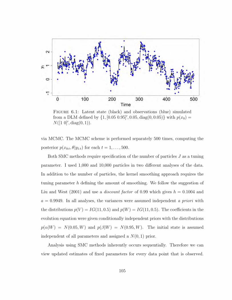
Figure 6.1: Latent state (black) and observations (blue) simulatedfrom a DLM defined by 1, [0.05 0.95]′, 0.05, diag(0, 0.05) with p(x0) =N([1 0]′, diag(0, 1)).
via MCMC. The MCMC scheme is performed separately 500 times, computing the
posterior p(x0:t, θ|y1:t) for each t = 1, . . . , 500.
Both SMC methods require specification of the number of particles J as a tuning
parameter. I used 1,000 and 10,000 particles in two different analyses of the data.
In addition to the number of particles, the kernel smoothing approach requires the
tuning parameter h defining the amount of smoothing. We follow the suggestion of
Liu and West (2001) and use a discount factor of 0.99 which gives h = 0.1004 and
a = 0.9949. In all analyses, the variances were assumed independent a priori with
the distributions p(V ) = IG(11, 0.5) and p(W ) = IG(11, 0.5). The coefficients in the
evolution equation were given conditionally independent priors with the distributions
p(α|W ) = N(0.05,W ) and p(β|W ) = N(0.95,W ). The initial state is assumed
independent of all parameters and assigned a N(0, 1) prior.
Analysis using SMC methods inherently occurs sequentially. Therefore we can
view updated estimates of fixed parameters for every data point that is observed.
105

Analysis performed in this fashion using 1,000 particles for both SMC methods can
be seen in Figure 6.2. In these plots, the MCMC analysis is used as a gold standard.
If one of the SMC algorithms is performing adequately it will match the MCMC
results with deviations from MCMC being due to either Monte Carlo variation or
biases due to the methodology. Monte Carlo variation is expected to be random
around the MCMC analysis as opposed to systematically biased over time.
Monte Carlo variation can be seen in these plots by noting, for example, the
sequential estimates for α. In particular, the kernel smoothing estimate of the 97.5%
quantile is initially low relative to the MCMC approach whereas around time 80
it is relatively high. Similarly the particle learning estimate of this same quantile
appears to be random around the MCMC results from time 0 to 150. Of course, there
is also Monte Carlo variation in the MCMC analysis and therefore it is unclear where
the truth lies. Nonetheless, it appears in these figures as though kernel smoothing
contains more Monte Carlo variation than the particle learning approach.
Of more immediate concern is bias due to the methodology. Due to the degen-
eracy issues caused by particle attrition, credible intervals estimated via these SMC
methods are expected to be narrower than the truth (or MCMC). Looking at the
plot for V in Figure 6.2, this degeneracy can be observed . Around time 140, the
credible intervals based on kernel smoothing appear to dramatically shrink relative
to MCMC. These intervals continue to shrink to almost a point at time 500. In a
similar manner, the particle learning approach shrinks beginning around time 200
and continues until 500, although not as severely as the kernel smoothing approach.
The easiest resolution to this degeneracy is to increase the number of particles
used in the SMC approaches. Figure 6.3 shows the same analysis but now with 10,000
particles rather than 1,000. An improvement over the previous analysis is obvious
although some degeneracy is still observed. Overall it still appears that the particle
learning approach outperforms kernel smoothing. If the length of the time series
106
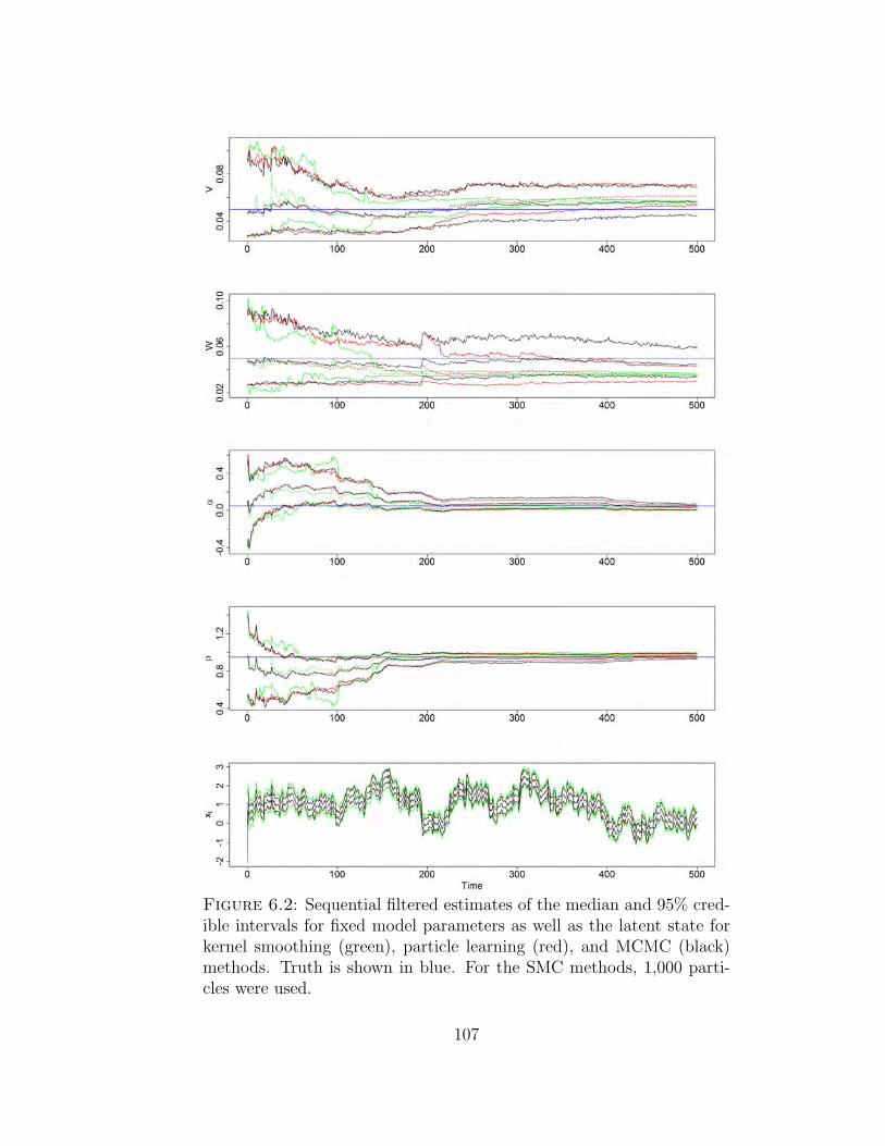
Figure 6.2: Sequential filtered estimates of the median and 95% cred-ible intervals for fixed model parameters as well as the latent state forkernel smoothing (green), particle learning (red), and MCMC (black)methods. Truth is shown in blue. For the SMC methods, 1,000 parti-cles were used.
107

Figure 6.3: Sequential filtered estimates of the median and 95% cred-ible intervals for fixed model parameters as well as the latent state forthe kernel smoothing (green), parameter learning (red), and MCMC(black) methods. Truth is shown in blue. For the SMC methods, 10,000particles were used.
108

were increased, I suspect more degeneracy would be observed in both approaches,
but more so in the kernel smoothing approach.
As mentioned earlier, the particle learning approach is more efficient computa-
tionally than the kernel smoothing approach. Since the particle learning approach
is theoretically more efficient and incurs less degeneracy, it is intuitive that where
possible we use this approach over the kernel smoothing approach. The next section
discusses a methodology that utilizes particle learning whenever possible and kernel
smoothing ideas otherwise.
6.3 Partial conditional sufficient structure
Unfortunately the model class that has a sufficient statistic structure is limited, e.g.
it does not include Gaussian models with nonlinear parameters such as studied in
Chapter 3 of this thesis. Hence, it is of interest to consider a wider class of models
that has a partial conditional sufficient structure. For these models, we subset fixed
parameters into two sets, θ and φ. Conditional on the latent states, data, and
parameter vector φ, the distribution for θ has a conditional sufficient structure, i.e.
p(θ|x1:t, y1:t, φ) = p(θ|st)
where st is a recursively defined sufficient statistic
st = S(st−1, xt, xt−1, yt, φ).
Clearly, models with conditional sufficient statistics represent a subclass of these
models.
Sequential parameter estimation is accomplished using the following factorization
p(θ, φ, xt, st|y1:t) = p(θ|st)p(φ, xt, st|y1:t).
This algorithm develops a particle approximation to the joint distribution of the
latent states, the sufficient statistics, and φ. Inference for θ is then performed off-
109

Table 6.3: Sequential Monte Carlo algorithm combining kernel smoothing andparticle learning in models with partial sufficient statistics. The algorithm as-sumes a particle approximation to p(xt−1, θ, φ, st−1|y1:(t−1)) is available, namely(xt−1, θ, φ, st−1)
(j), j ∈ 1, 2, . . . , J.
1. Reweight particles according to w(j)t ∝ p(yt|x(j)
t−1, φ(j), θ(j)).
2. Approximate p(φ|y1:t) ≈∑J
j=1N(φ|m(j)t , h2Mt) where m
(j)t = aφ(j) + (1− a)φt
and
φt =J∑j=1
w(j)t φ(j) and Mt =
J∑j=1
w(j)t (φ(j) − φt)(φ
(j) − φt)T .
Set j = 1.
3. Sample an index k = w(j)t and draw a new value for φ(j) ∼ N(φ|m(k)
t , h2Mt).
4. Propagate the state according to x(j)t ∼ p(xt|x(k)
t−1, θ(k), φ(j), yt).
5. Update the sufficient statistics according to s(j)t = S(s
(k)t−1, x
(j)t , yt, φ
(j)).
6. Sample a set of auxiliary parameters according to θ(j) ∼ p(θ|s(j)t ).
7. If j < J , set j = j + 1 and return to step 4.
line conditional on the sufficient statistics at the associated time. The full algorithm
is shown in Table 6.3. This provides a framework for reducing degeneracy as much
as possible with applicability to this wide model class.
6.4 Example motivated by pathway studies in systems biology
As an illustration of this method, consider the model shown in equation (4.6). This
model contains the parameter β which appears nonlinearly in the evolution equation
for the target protein. Due to this nonlinearity, this model cannot be analyzed by the
particle learning framework discussed in Section 6.2.2. Adding a kernel smoothing
approach, as discussed in Section 6.3, allows sufficient statistics to be used for all
110

parameters other than β.
The same data and priors as those used in Section 4.6.1 are used in this analysis.
Due to k, α, ψ, φ having truncated normal priors, a slightly modified version of the
algorithm described in Table 6.3 is required. Step 5 and 6 are modified by a Gibbs-
style step. Instead of updating all sufficient statistics in block and then sampling new
values for each parameters, the sufficient statistic for each parameter will be updated
and then a new value will be sampled prior to updating the sufficient statistics for
other model parameters.
To fix this idea, suppose two fixed parameters, θ1 and θ2, are to be updated along
with their sufficient statistics. At time t − 1, particle i contains draws for the pa-
rameters, θ(i)1,t−1 and θ
(i)2,t−1 and their sufficient statistics s
(i)1,t−1 and s
(i)2,t−1, respectively,
and where the subscript indicates that these parameters and their sufficient statistics
were determined at time t−1. First, update s(i)1,t−1 conditional on θ
(i)2,t−1 to obtain s
(i)1,t
and sample θ(i)1,t ∼ p(θ1|s(i)
1,t). Second, update s(i)2,t−1 conditional on θ
(i)1,t to obtain s
(i)2,t
and sample θ(i)2,t ∼ p(θ2|s(i)
2,t). If more than two fixed parameters are to be updated,
conditioning on the most recently sampled parameters as in Gibbs sampling provides
the updating.
I analyzed the data using the SMC algorithm described in Table 6.3 where φ = β,
θ = k, α, ψ, µ0, µ1, φ, σm, σa, σx, h = 0.1004, and a = 0.9949. The modification
described in the previous paragraph was used to update the sufficient statistics for
k, α, ψ, and σx in sequence as well as µ0, µ1, φ, and σa. Runs were performed
as described in Table 6.3, but showed high multi-modality presumably due to high
Monte Carlo variation induced by the multinomial sampling in Step 3. Therefore
Step 3 in this table was also replaced with a residual sampling. If J particles are
required, residual sampling replicates each particle bJw(j)t c times where bxc denotes
the largest integer less than x and w(j)t is the normalized weight. Then multinomial
111

samples are taken proportional to Jw(j)t − bJw(j)
t c for a total of J particles.
The algorithm was run using 20,000 particles although a 100,000 particle run was
also performed yielding similar results. These runs can be completed in a matter of
a couple of minutes on a 3.2GHz computer, but the 100,000 particle run required
4.5Gb of memory. This requirement could be lessened if particle histories are not
stored.
Posterior estimates for model parameters are investigated using the final filtered
distribution shown in Figure 6.4 which can be compared to the MCMC results shown
in Figure 4.18 reproduced as Figure 6.5. The ranges of the axes in these plots were
made equal to the ranges in the MCMC analysis for ease of comparison. The poste-
riors in these plots generally agree with the MCMC analysis, but discrepancies exist.
In particular, many of the histograms are multi-modal where a smooth distribution
is expected. These differences are most likely due to particle attrition.
This analysis implements an SMC approach to analyzing a 10-dimensional fixed
parameter vector along with a 2-dimensional state. Compared to the MCMC anal-
ysis, the results of the SMC analysis are not as convincing and runs with larger
numbers of particles are necessary to reduce the degeneracy observed. Larger runs
are restricted by memory currently available in computers and therefore meticulous
coding is required to maximize the number of particles available.
6.5 Summary
In this chapter, I discussed the basics of sequential Monte Carlo and outlined two
existing approaches to reducing weight degeneracy in SMC algorithms with fixed,
but unknown parameters. Through an example, I illustrated the benefits of using
the particle learning approach over the kernel smoothing with APF approach when it
is possible. I introduced an algorithm that utilizes sufficient statistics where possible
112

Figure 6.4: Model of (4.7): Histograms of marginal posterior estimates(blue), prior (green), and true value (red) for fixed model parameters basedon an SMC analysis.
Figure 6.5: Model of (4.7): Histograms of marginal posterior estimates(blue), prior (green), and true value (red) for fixed model parameters basedon an MCMC analysis.
113

and kernel smoothing otherwise to reduce degeneracy for fixed parameters. Finally,
I implemented this algorithm on a biology example and compared the results with
an MCMC analysis.
Bayesian approaches to sequential estimation of both states and fixed parameters
currently suffer from degeneracy of particles representing fixed parameters. Sufficient
statistics can be used in some models to reduce this degeneracy. The approach
discussed in this chapter attempt to alleviate this degeneracy by combining kernel
smoothing and sufficient statistics ideas but ultimately still suffer as t increases. One
approach I am currently exploring that may alleviate this problem is to freeze the
sufficient statistics at some lag L prior to the current time t. Freezing the sufficient
statistics introduces bias, but combats the degeneracy issue by not resampling the
entire particle history. This approach has been used in the expectation-maximization
framework for maximum likelihood estimation (Olsson et al., 2008).
114
7
Sequential Monte Carlo methods for influenzaoutbreak detection using Google flu activity
Estimate
Public health surveillance for infectious diseases attempts to quickly recognize emerg-
ing outbreaks whether from natural or bioterrorism sources and alert public health
officials. The data sources for these surveillance system are numerous, including
emergency department visits, poison control center hotlines, and over-the-counter
medicine sales. For reviews of these and other sources, see Thacker and Berkelman
(1988) and Thacker and Stroup (1994).
Statistical methods are widely used for analyzing these data streams. Initial work
has focused on statistical process control approaches including thresholds (Serfling,
1963; Watier et al., 1991; Farrington et al., 1996), moving averages (Stern and Light-
foot, 1999), exponentially weighted moving averages (Williamson and Hudson, 1999),
cumulative sums (Rossi et al., 1999; Frisn, 2003), and autoregressive integrated mov-
ing averages (Choi and Thacker, 1981; Helfenstein, 1986; Stroup et al., 1989; Watier
et al., 1991; Reis and Mandl, 2003). For influenza, the Centers for Disease Con-
trol and Prevention (CDC) currently uses Serfling’s method (Serfling, 1963) which
115
attempts to determine a national baseline level of flu activity and a threshold for
declaring an influenza epidemic. As pointed out by Martınez-Beneito et al. (2008),
such threshold methods have serious drawbacks when baselines change over time
or when the interest is in regional rather than national outbreaks. For reviews of
these methods see LeStart (2005) and Burkom (2007). Many of these algorithms are
implemented in the R-package surveillance (Hohle, 2007).
Time series analysis using dynamic models has increased in popularity recently.
Inference is performed either on a switching Markov state that indicates whether
the area under observation is currently in an epidemic or on an underlying state
that indicates the prevalence of the disease. For early reviews in this area, see
Woodall (1997), Frisn (2003), and Sonesson and Bock (2003). Maximum likelihood
approaches to inference in these models can be found in Le Strat and Carrat (1999),
Rath et al. (2003), Cooper and Lipsitch (2004), and Porter et al. (2008). For Bayesian
approaches in hidden Markov models, see Madigan (2005), Cowling et al. (2006),
Sebastiani et al. (2006), and Martınez-Beneito et al. (2008). In particular, Cowling
et al. (2006) find that a DLM outperforms a cumulative sum approach in monitoring
influenza in Hong Kong and the US.
For real public health surveillance, more sophisticated models will be required
that incorporate the natural spatial and multivariate data sources. Space-time mod-
els are a natural extension of time series models when data is being collected on
regional units such as states or counties. Examples of these models and their ap-
plications can be found in Svensson and Lindback (2002), Mugglin et al. (2002),
Knorr-Held and Richardson (2003), Rogerson and Yamada (2004), Madigan (2005),
and Niemi et al. (2008a). Another natural extension is to multivariate data streams
such as those found in Held et al. (2005) and Sebastiani et al. (2006). From all
of these surveillance systems, public health decisions are the end goal. Merl et al.
(2008) discuss a statistical framework for choosing optimal intervention strategies.
116

In this chapter, I consider univariate time series data with information on out-
breaks, and attempt to quickly recognize those outbreaks. I build a dynamic model
that contains a Markov switching process identifying the epidemic. The novelty lies
in the dynamic model construction, the data source, and applying sequential Monte
Carlo algorithms for inference. SMC was suggested in Martınez-Beneito et al. (2008),
but the analysis was not performed.
7.1 Google flu activity estimate
Influenza is infection of the lungs and airways by one of the influenza viruses. It can
cause a fever, sore throat, cough, headache, muscle aches, and a general feeling of
illness. Influenza epidemics occur every year during the late fall and early winter.
These normal epidemics result in an estimated 20 to 50 million cases of influenza and
influenza-like illness, resulting in over 100,000 hospitalizations, over 36,000 influenza-
related death, and incur 1 to 3 billion U.S. dollars in direct medical costs and 10 to
15 billion dollars in indirect costs. Baccam et al. (2006). During pandemics these
numbers can be much higher. Therefore influenza surveillance is an important task
in public health.
Recently researchers have identified a new source of data for quick determination
of the influenza status across the entire US (Ginsberg et al., 2009). This data source
involves measurements of the number of search engine queries for terms associated
with influenza and its symptoms. CDC has an alternative approach based on a
sentinel network of physicians who report to the CDC on the number/percentage of
patients who are symptomatic of the flu. The search engine query data was shown
to provide an accurate approximation to the CDC sentinel data. The benefit of
the search engine query data is the promptness of the reporting which can be up
to two weeks earlier than that of the sentinel network. In fact, according to the
authors, search engine query data can be reported with a “lag of about one day.”
117

Figure 7.1: Weekly reported Google flu activity estimate for NorthCarolina influenza season (top) and first order differences (bottom) frommid-2004 until mid-2008.
Therefore, this data source may be more practical for use by public health officials
in determining regional intervention decisions.
Figure 7.1 shows an influenza estimate for the state of North Carolina over the
past five years. It is clear that near the middle of each year influenza peaks, but the
severity, number, and exact timing of the peaks varies from year to year. From a
public health perspective an ideal scenario is to build a model that accurate predicts
both the severity and location of these peaks. In this chapter, I build a model and
analysis for online determination of the probability of currently being in an epidemic.
118

7.2 A model for influenza epidemic detection
Following Martınez-Beneito et al. (2008), I model the one-step differences in obser-
vations. For the North Carolina data, these differences are shown in the bottom half
of Figure 7.1. Similar to their argument, I model the epidemic and non-epidemic
phases using a hidden Markov model (Carvalho and Lopes, 2007). Let Yt indicate
the flu activity estimate at time t minus the flu activity estimate at time t − 1. I
augment the model of Martınez-Beneito et al. (2008) to create a dynamic model.
The observation equation is
Yt ∼ N(Xt, σ2y)
where Xt is the latent state of the system. The evolution equation for the state Xt
is dependent on the indicator for epidemics Zt through
Xt|Zt = 1 ∼ N(ρXt−1, σ2x)
and P (Xt = 0|Zt = 0) = 1. In an epidemic, the state is an autoregressive process
of order one. The epidemic indicator is a two-state Markov chain with transition
probability p0 and p1 to remain in a non-epidemic and epidemic phase, respectively.
Although this model is very close in spirit with Martınez-Beneito et al. (2008), I be-
lieve it offers a more natural interpretation. In particular, σ2y represents the variance
associated with measurement error of the observations and Xt is the rate of change
of the epidemic.
This model is a modification of the state-of-the-art model of Martınez-Beneito
et al. (2008) for influenza detection. Nonetheless, it is clear from visual inspection of
Figure 7.1 that this model of first differences is inadequate. In particular, rather than
an autoregressive process occurring during outbreaks, the first differences appear to
have a more complicated structure due to the negative correlations observed. Options
119

for more accurately modeling these first differences include allowing for negative
autoregressive parameters or increasing the order of the autoregressive process. The
focus here is on the applicability of SMC methods to detection of influenza outbreaks
and therefore building of more accurate models is beyond the scope of this chapter.
7.3 Sequential Monte Carlo methods for influenza detection
The sequential approach adopted by Martınez-Beneito et al. (2008) was to run a
full MCMC for each time point. Therefore the analysis at time t − 1 has no affect
on the analysis at time t despite the only difference between these analyses being
the one extra observation at time t. SMC algorithms use all information up to
time t − 1 in accomplishing the analysis at time t. Therefore, SMC algorithms are
computationally efficient compared to sequential MCMC analyses.
This section introduces three approaches to SMC for Bayesian analysis of the
model described in the previous section. The first implements the particle learning
approach of Carvalho et al. (2008) utilizing the Gibbs step as described in Section
6.4. The second builds on the kernel smoothing approach in West (1993b) and Liu
and West (2001) by taking advantage of the exact sampling framework of Carvalho
et al. (2008). The third uses the methodology of Section 6.3 which combines kernel
smoothing and particle learning.
7.3.1 Particle learning for influenza detection
The particle learning framework of Carvalho et al. (2008) can be applied to the model
of Section 7.2. Define the parameter vector to be θ = (σ2y , σ
2x, ρ, p0, p1), then particle
learning has three requirements:
1. P (Yt|Xt−1, Zt−1, θ) can be evaluated,
2. P (Xt, Zt|Yt, Xt−1, Zt−1, θ) can be sampled, and
120

3. P (θ|y1:t, x1:t, z1:t) = P (θ|st) for some sufficient statistic st whose dimension
does not depend on t.
The first requirement is satisfied noting the following identities:
P (Yt|Xt−1 = 0, Zt−1 = 0) = p0N(yt|0, σ2y) + (1− p0)N(yt|0, σ2
y + σ2x),
P (Yt|Xt−1 = xt−1, Zt−1 = 1) = (1− p1)N(yt|0, σ2y) + p1N(yt|ρxt−1, σ
2y + σ2
x).
The predictive distribution for the next observation is a two-component mixture of
Gaussians. If currently in an epidemic, then the predictive distribution sums over the
two possibilities: staying in an epidemic or moving out of one. If currently not in an
epidemic, then the predictive distribution sums over the complementary possibilities:
staying out of an epidemic or moving into one.
The second requirement is satisfied noting the identity
P (Xt, Zt|Yt, Xt−1, Zt−1, θ) = P (Xt|Yt, Xt−1, Zt, θ)P (Zt|Yt, Xt−1, Zt−1, θ).
This suggests a joint sampling strategy for Xt and Zt where Zt is sampled first and
then conditional on Zt, Xt is sampled. Since Zt is binary, the conditional posterior
probabilities are easy to compute and are given in equations (7.1) and (7.2).
P (Zt = 0|Yt = yt, Xt−1 = 0, Zt−1 = 0, θ) =
p0N(yt|0, σ2y)
p0,1N(yt|0, σ2y) + p0,1N(yt|0, σ2
y + σ2x)
(7.1)
P (Zt = 1|Yt = yt, Xt−1 = xt−1, Zt−1 = 1, θ) =
p1N(yt|ρxt−1, σ2y + σ2
x)
p1N(yt|ρxt−1, σ2y + σ2
x) + p1,0N(yt|0, σ2y). (7.2)
If Zt = 0 is sampled, then Xt is trivially 0, but if Zt = 1 then sampling from the
conditional filtered distribution for Xt is accomplished according to
P (Xt|Yt = yt, Xt−1 = xt−1, Zt = 1, θ) = N(gt, Gt) (7.3)
121
where gt = Gt
(ytσ
−2y + ρxt−1σ
−2x
)and Gt = (σ−2
y + σ−2x )−1.
The third requirement would be satisfied if these priors are assumed at time
t − 1: σ2y ∼ IG(at−1, At−1), σ
2x ∼ IG(bt−1, Bt−1), ρ|σ2
x ∼ N(ct−1, σ2xCt−1), p0 ∼
Be(dt−1, Dt−1), and p1 ∼ Be(et−1, Et−1). The prior for ρ is unrestricted, but Martınez-
Beneito et al. suggest restricting ρ to (0, 1) to maintain stationary of the x process
and positive correlations. Therefore a prior of the form ρ|σ2x ∼ N(ct−1, Ct−1)I(0 <
ρ < 1) is chosen.
This choice requires a Gibbs step to be introduced as it was in Section 6.4. The
idea is to first update the sufficient statistics for ρ and draw a sample. Then, update
the sufficient statistics for all other parameters conditional on this new value for ρ and
sample the other parameters. Once yt is observed and xt and zt have been jointly
sampled using the procedure above, the sufficient statistics for ρ can be updated
using the updating rules
ct = Ct
(ztxtxt−1
σ2x
+ct−1
Ct−1
), Ct =
(ztx
2t−1
σ2x
+1
Ct−1
)−1
. (7.4)
The inclusion of zt indicates that ρ is only updated when the state of the system is
in an epidemic at time t. Once ρ has been sampled from N(ρ|ct, Ct), the following
rules can be used to update the remaining sufficient statistics
at = at−1 + 1/2, At = At−1 +(yt − xt)
2
2,
bt = bt−1 + zt/2, Bt = Bt−1 + zt(xt − ρxt−1)
2
2, (7.5)
dt = dt−1 + zt(1− zt−1), Dt = Dt−1 + (1− zt)(1− zt−1),
et = et−1 + ztzt−1, Et = Et−1 + (1− zt)zt−1.
The sufficient statistic vector is then st = (at, At, bt, Bt, ct, Ct, dt, Dt, et, Et) and off-
line inference concerning the parameters can be accomplished using P (θ|st). The
model and analysis is fully-specified by assuming a prior distribution for X0 ∼
122
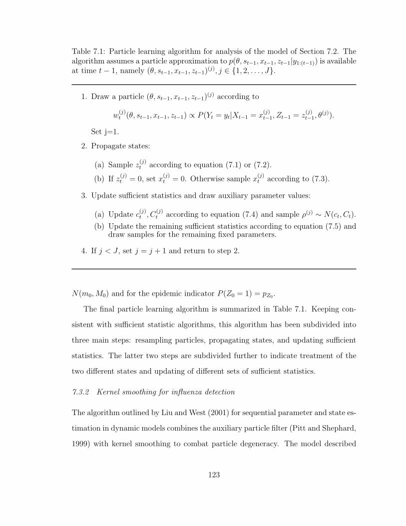
Table 7.1: Particle learning algorithm for analysis of the model of Section 7.2. Thealgorithm assumes a particle approximation to p(θ, st−1, xt−1, zt−1|y1:(t−1)) is availableat time t− 1, namely (θ, st−1, xt−1, zt−1)
(j), j ∈ 1, 2, . . . , J.
1. Draw a particle (θ, st−1, xt−1, zt−1)(j) according to
w(j)t (θ, st−1, xt−1, zt−1) ∝ P (Yt = yt|Xt−1 = x
(j)t−1, Zt−1 = z
(j)t−1, θ
(j)).
Set j=1.
2. Propagate states:
(a) Sample z(j)t according to equation (7.1) or (7.2).
(b) If z(j)t = 0, set x
(j)t = 0. Otherwise sample x
(j)t according to (7.3).
3. Update sufficient statistics and draw auxiliary parameter values:
(a) Update c(j)t , C
(j)t according to equation (7.4) and sample ρ(j) ∼ N(ct, Ct).
(b) Update the remaining sufficient statistics according to equation (7.5) anddraw samples for the remaining fixed parameters.
4. If j < J , set j = j + 1 and return to step 2.
N(m0,M0) and for the epidemic indicator P (Z0 = 1) = pZ0 .
The final particle learning algorithm is summarized in Table 7.1. Keeping con-
sistent with sufficient statistic algorithms, this algorithm has been subdivided into
three main steps: resampling particles, propagating states, and updating sufficient
statistics. The latter two steps are subdivided further to indicate treatment of the
two different states and updating of different sets of sufficient statistics.
7.3.2 Kernel smoothing for influenza detection
The algorithm outlined by Liu and West (2001) for sequential parameter and state es-
timation in dynamic models combines the auxiliary particle filter (Pitt and Shephard,
1999) with kernel smoothing to combat particle degeneracy. The model described
123

Table 7.2: Kernel smoothing algorithm for analysis of the model of Section 7.2. Thealgorithm assumes a particle approximation to p(θ, xt−1, zt−1|y1:(t−1)) is available attime t− 1, namely (θ, xt−1, zt−1)
(j), j ∈ 1, 2, . . . , J.
1. Reweight particles according to
w(j)t (θ, xt−1, zt−1) ∝ P (Yt = yt|Xt−1 = x
(j)t−1, Zt−1 = z
(j)t−1, θ
(j))
2. Calculate the kernel density approximation to the posterior distribution for θ,
namely p(θ|y1:t) =∑J
j=1N(θ|m(j)t , h2Mt) where m
(j)t = aθ(j) + (1 − a)θ, θ =∑J
j=1w(j)t θ(j), Mt =
∑Jj=1w
(j)t (θ − θ)(θ − θ)′, and h =
√1− a2 is typically
small. Set j=1.
3. Sample an indicator k ∈ 1, . . . , J with probability proportional to w(j)t and
sample θ(j) ∼ N(m(k)t , h2Mt).
4. Sample z(j)t according to (7.1) or (7.2) using z
(k)t−1.
5. If z(j)t = 0, set x
(j)t = 0. Otherwise sample x
(j)t according to (7.3) using x
(k)t−1
and θ(j).
6. If j < J , set j = j + 1 and return to step 3.
in Section 7.2 for influenza detection allows for a more efficient approach due to the
analytical tractability of P (Yt|Xt−1, Zt−1, θ) and P (Xt, Zt|Yt, Xt−1, Zt−1, θ) as shown
in the previous section. This allows for exact sampling of particles at each time point
(Carvalho et al., 2008). Once exact sampling has been accomplished, new parameters
can be sampled using the kernel smoothing ideas of West (1993b).
The algorithm that combines exact sampling with kernel smoothing is provided
in Table 7.2. A difference from the algorithm outlined in Liu and West (2001) is that
kernel smoothing occurs after particle reweighting. Therefore, the kernel smoothed
distribution is an approximation of the posterior of the fixed parameters at time t
rather than an approximation of the prior at that time.
124

7.3.3 Kernel smoothing with particle learning applied to influenza data
The previous two sections have developed particle filtering algorithms for sequential
parameter and state estimation using kernel smoothing and sufficient statistics sep-
arately to combat particle degeneracy. This section combines these two approaches
by regenerating samples for ρ using kernel smoothing and using sufficient statistics
for all other parameters. This approach was utilized in Section 6.4 for a nonlinear
parameter allowing sufficient statistics to be used for all other parameters. The no-
tation θ−ρ is used to represent the vector of fixed parameters excluding ρ. In this
section, the sufficient statistics are sufficient statistics for θ−ρ.
The algorithm describing this approach for use in influenza surveillance is in Table
7.3. Compared with the kernel smoothing approach of Table 7.2 which required kernel
density approximation in five dimensions, this algorithm only requires kernel density
approximation in one. It is therefore expected, based on the comparison of kernel
smoothing and particle learning performed in Section 6.2.3, that this algorithm would
perform superior to the kernel smoothing of all parameters. It is unclear how this
algorithm will fair relative to the particle learning with a Gibbs step of Table 7.1.
7.4 Analysis of Google flutrend data
The algorithms of the previous section are used to the analyze the North Carolina
Google flu activity estimate shown in Figure 7.1. Initial priors for model parameters
were all assumed independent and diffuse. In particular σ2y ∼ IG(2, 0.12), σ2
x ∼
IG(1, 52), ρ ∼ N(0.5, 0.252)I(0 < ρ < 1), p0 ∼ Be(9, 1), p1 ∼ Be(9, 1), p(x0) =
N(0, 1), and p(z0 = 1) = 1/100. I used 10,000 particles over this 4-year time-
frame that included a total of 212 observations. For both algorithms that utilized
kernel smoothing, h = 0.1004. Running the algorithms multiple times resulted in
equivalent inferences within Monte Carlo variation indicating that degeneracy in this
125

Table 7.3: Algorithm combining kernel smoothing with particle learning foranalysis of the model of Section 7.2. The algorithm assumes a particle ap-proximation to p(θ−ρ, ρ, st−1, xt−1, zt−1|y1:(t−1)) is available at time t − 1, namely(θ−ρ, ρ, st−1, xt−1, zt−1)
(j), j ∈ 1, 2, . . . , J.
1. Reweight particles according to
w(j)t (θ−ρ, ρ, st−1, xt−1, zt−1) ∝ P (Yt = yt|Xt−1 = x
(j)t−1, Zt−1 = z
(j)t−1, θ
(j)−ρ, ρ)
2. Calculate the kernel density approximation to the posterior distribution for ρ,
namely p(ρ|y1:t) =∑J
j=1N(ρ|m(j)t , h2Mt) where m
(j)t = aρ(j) + (1 − a)ρ, ρ =∑J
j=1w(j)t ρ(j), Mt =
∑Jj=1w
(j)t (ρ(j) − ρ)2, and h =
√1− a2 is typically small
Set j=1.
3. Sample an indicator k ∈ 1, . . . , J with probability proportional to w(j)t and
sample ρ(j) ∼ N(m(k)t , h2Mt).
4. Sample z(j)t according to (7.1) or (7.2) using z
(k)t−1.
5. If z(j)t = 0, set x
(j)t = 0. Otherwise sample x
(j)t according to (7.3) using x
(k)t−1
and θ(k)−ρ and ρ(j).
6. Update s(j)t according to (7.5) for all distributions except that for ρ.
7. Draw θ(j)−ρ ∼ P (θ−ρ|s(j)
t ).
8. If j < J , set j = j + 1 and return to step 3.
model using this many particles over this many observations was not an issue.
Sequential parameter estimates are shown in Figure 7.2. In this set of plots, the
effect of no epidemic is clear. In particular, no information is gained for parameters
σx, ρ, and p1 and therefore the medians and credible intervals are flat (outside of
Monte Carlo variation). Additionally, the parameter p0 has credible intervals that
are converging to 1 prior to any epidemic. As soon as an epidemic is observed,
more uncertainty is evident for p0 while the 3 epidemic parameters show immediate
learning.
126

Figure 7.2: Sequential pointwise 95% credible intervals and means forfixed parameters using the kernel smoothing (blue), particle learning(green), and kernel smoothing with particle learning (red) approacheson North Carolina Google flu activity estimate.
127
The analysis by the particle learning (PL) and the particle learning with kernel
smoothing (PL+KS) show approximately the same results. The kernel smoothing
(KS) approach appears to degenerate rapidly. This appears to be caused by the
sequential estimation of the observation error σy. For this parameter, all three meth-
ods agreed initially. At the end of 2004, the particle learning based approaches infer
a much larger observation error compared with the KS approach. Presumably the
degeneracy observed in the KS approach is due to the inability to sample particles
with large values of σy while simultaneously having reasonable values for all other
parameters.
Of primary interest to public health officials is the probability of an influenza
outbreak. Figure 7.3 shows the sequential estimate for the current probability of
being in an influenza outbreak. All three methods appear similar in their probability
estimation despite their differences in parameter estimation.
7.5 Summary
This chapter built a dynamic model for influenza detection and analyzed North Car-
olina Google flu activity estimate using a variety of SMC procedures. Modifications
to existing SMC algorithms were made to combat degeneracy in both parameter
and state estimation using a combination of exact sampling, kernel smoothing, and
sufficient statistics. Use of sufficient statistics for all or part of the parameter vector
appears to be beneficial in reducing degeneracy of sequential parameter estimates.
A similar version of this model appears to have worked well for Martınez-Beneito
et al. (2008) when analyzing influenza data from sentinel data in Comunitat Valen-
ciana, Spain. The model can clearly be improved by explicitly modeling the negative
autocorrelations observed in the first differences of influenza activity. Future work
will focus on these modeling choices as well as incorporating spatial information and
influenza mechanisms.
128

Figure 7.3: Sequential estimates of current epidemic probability basedon kernel smoothing (blue), particle learning (green), and kernel smooth-ing with particle learning (red) approaches with scaled North CarolinaGoogle flu activity estimate (gray).
129

8
Additional discussion and future research
I have discussed a number of computational methods for Bayesian analysis in dy-
namic models. The methods have focused on computational efficiency in the presence
of unknown fixed parameters as well as states. I applied these methods to real and
simulated data sets in the diverse fields of systems biology, quantitative finance, and
disease surveillance. These methods outperformed standard alternative methods in
the examples tested. These are significant advances but the opportunities for future
research are abundant.
8.1 Adaptive mixture modeling
The adaptive mixture modeling approach described in Chapters 2 and 5 provides
methodology for jointly sampling the latent state vector process in nonlinear non-
Gaussian models. These methods could be improved by more efficient quantile esti-
mation, generalizing to multivariate states, dynamic choice for the number of mixture
components, and increasing the effective acceptance rate.
The AM4 method requires computing quantiles of mixtures of Gaussians. This is
currently accomplished through a relatively brute force approach based on finding a
130

zero for the function f(x) = q−∑J
j=1 pjΦ(x|mj, Cj) where Φ(x|m,C) is the cumula-
tive distribution function for a Gaussian with mean m and variance C evaluated at
x. This zero-finding is performed for J-quantiles for each regeneration. At minimum
a more efficient approach would utilize the monotonic nature of the function in both
x and q. At best, one would utilize the fact that I am always finding quantiles of
mixtures of Gaussians as opposed to arbitrary functions.
My approach to jointly sampling a latent state vector in nonlinear non-Gaussian
models is currently limited to univariate states. Generalizing the approach to multi-
variate states requires either being able to define and calculate multivariate quantiles
or avoiding them altogether. A possible approach used by Sorenson and Alspach
(1971) is to approximate each evolution error distribution by a mixture of precise
Gaussians. If the initial prior was composed of J0 mixture components and I ap-
proximate the evolution error distribution at time t by Jt mixture components, then
at time T approximation of the state posterior would require∏T
t=0 Jt mixture com-
ponents which would be a prohibitively large number. Sorenson and Alspach (1971)
suggest pruning/combining components to fix either a constant number of compo-
nents throughout the procedure or a maximum error in each step. If the evolution
error distribution is constant through time this could provide an appealing approach,
but if this error distribution changes the procedure requires approximating each
unique distribution with a new mixture of Gaussians which would be computational
intensive. The strategy opted for in this thesis alternates draws from each univariate
state process using Gibbs sampling. This strategy was very effective in the examples
studied.
The AM4 methodology currently sets the number of mixture components at time
zero and runs through the algorithm. As a practical matter, this number is increased
until a suitable acceptance rate is observed. A more efficient and less user intensive
approach would adapt at each step by dynamically choosing the number of mixture
131

components needed for that step. This need is clearly seen when discussing the
nonlinear Gaussian examples. On one hand, if the function happens to be fairly linear
over the mass of the prior, then only one component is need to accurately capture
the nonlinearity. On the other hand, if the function is highly nonlinear, then many
components will be needed for accurate approximations. It is likely that the number
of mixture components needed for a specific acceptance rate is heavily influenced by
one (or a few) highly nonlinear times. Dynamically learning the number of mixture
components could reduce the number of components needed, but will require many
evaluations of the function and perhaps its derivative.
In situations where AM4 has low acceptance rate and therefore induces poor
mixing, an improvement to the MCMC is to repeat the Gibbs step for sampling latent
states multiple times for each sweep of the MCMC. The AM4 method is composed of
three main steps: forward filtering, backward sampling, and Metropolis acceptance
probability calculation. Forward filtering is relatively computational expensive, but
in this scenario would only be run once for each MCMC sweep. Backward sampling
and Metropolis acceptance probability calculation could then be done multiple times
with relatively little computational overhead. The number of repeats could be fixed,
random, or even learned adaptively up to some MCMC iteration. Perhaps a more
efficient approach would be to incorporate delayed rejection (Mira, 2001) which would
allow the algorithm to continue as soon as a sample is accepted. This is particularly
appealing in an independence sampler such as AM4.
8.2 Sequential Monte Carlo for fixed parameters
In Chapter 6 I introduced two SMC algorithms for simultaneous state and parameter
estimation in dynamic models. I used a simulation example to argue that the particle
learning approach (Carvalho et al., 2008) is less susceptible to the degeneracy issue
compared to the kernel smoothing plus APF approach (Liu and West, 2001). Un-
132

fortunately, the particle learning approach is restricted to a specific class of models
whereas the alternative approach is completely general. One future area of focus is
to understand whether the gains by using particle learning are attributable to exact
sampling, sufficient statistics, or the combination of the two.
I then introduced a novel algorithm that adds kernel smoothing to the particle
learning approach for parameters that do not have a sufficient statistic structure.
Directions for future work include adding sufficient statistics to the kernel smoothing
plus APF approach, understanding the importance of resampling scheme in the exact
sampling framework, and researching biased approaches using sufficient statistics
that have less (or no) degeneracy issues.
The novel SMC method outlined in this thesis is restricted to the class of models
where exact sampling is possible, i.e., those models where the integral∫p(yt|xt, θ)p(xt|xt−1, θ)dxt
is analytically tractable. An approach that avoids this integration when it is in-
tractable while still maintaining reasonably uniform importance weights is APF. A
new completely general, yet efficient SMC algorithm would add sufficient statistics
where applicable to the approach of Liu and West (2001). When no parameters have
a sufficient statistic structure, the algorithm would reduce to that of Liu and West,
but when possible the use of sufficient statistics should reduce the degeneracy issue.
Currently, the exact sampling procedure of Carvalho et al. (2008) uses multino-
mial resampling prior to propagation. Use of other resampling procedures such as
the use of residual sampling in Section 6.4 should reduce the degeneracy issue since
they reduce the Monte Carlo variability introduced in the resampling step.
As mentioned in the summary of Chapter 6, if unbiased specification is relaxed in
SMC algorithms, if my be possible to develop algorithms with lower mean squared
error (MSE) for estimation of medians or credible intervals. The approach suggested
133
is to use a fixed lag at which the sufficient statistics are frozen. This has been
used successfully both practically and theoretically in the expectation-maximization
literature for finding maximum likelihood estimates in nonlinear dynamic models
(Olsson et al., 2008).
8.3 Systems and synthetic biology
Through the use of microarrays and other high-throughput technology, scientists
are beginning to understand the interconnectedness of DNA, RNA, and proteins
within living cells. From these data, graphcs can be built that represent pathways of
interaction between these components. Part of this thesis was devoted to Bayesian
methods for analysis that aims to understanding the dynamics of a given subgraph to
answer biological questions. For example: How quickly does the activation of protein
B by protein A occur? If we reduce the association strength of two proteins by half,
what will be the affect on the system? If we design a drug bind with protein C,
will that stop the tumor progression? What role does intrinsic variation play in cell
differentiation? To answer these types of questions a statistical model is necessary to
describe the system and the parameters in this model need to be estimated by data.
Future work in this area will focus on experimental design, evolution equations that
reflect mechanisms, positive evolution error distributions, and incorporating multiple
data sources.
The experimental design front seeks to isolate particular parameters in a statisti-
cal model. Using Bayesian techniques allows for using posteriors from one experiment
to build priors for the next. This will allow learning to progress in a manner that is
consistent with the way science knowledge is gained. In so doing bigger and more so-
phisticated models can be constructed to represent the complexity that exists within
living cells.
The biological models studied in this thesis were built such that the observation
134

equation was a noisy measurement of a true fluorescence level. This then requires the
state to live in the domain of fluorescence. More appealing is a state that lives in the
more natural domain of either protein concentration or number of molecules. In turn,
this requires the observation equation to reflex the transformation of the state to the
observation. In fluorescence microscopy experiments this may lead to logistic type
curves since there is a minimum and maximum possible fluorescence. This would
make priors and posteriors for evolution parameters more naturally interpretable by
scientists since they are accustomed to thinking in terms of concentration or numbers
of molecules.
Now that the evolution equation represents concentration or numbers of molecules
it is more natural to require the evolution distribution to be positive, e.g. gamma
or Poisson. A gamma autoregressive process when decomposed into the sum of a
gamma random variable (r.v.) plus a beta r.v. times the current state is quite natural
in this context. The beta r.v. can be interpreted as the percent remaining from the
previous time point and the gamma r.v. as the amount produced. These models
more naturally handle low numbers of molecules as there is no chance of a negative
value.
In addition to more accurate modeling of experiments such as time-lapse fluores-
cence microscopy is to combine multiple data sources. A natural complement for the
microscopy experiments is flow cytometry. In a flow cytometry experiments, enor-
mous amounts of data are obtained on the marginal distribution of protein concen-
tration, but no information is available about the dynamics. Building dynamic mod-
els where the state represents either protein concentration or number of molecules
would allow for simultaneous analysis of both experiments. The observation equa-
tions would then represent the actual observation process involved. Combining these
and other data sources has the potential to dramatically improve knowledge about
these systems.
135

8.4 Disease surveillance
To borrow a phrase, in a world that is hot, flat, and crowded diseases are certainly
going to be a public health concern. Diseases can be naturally occurring such as
influenza, SARS, or bird flu, but then can also be human caused such as an anthrax
attack, thickening milk with melamine, or releasing peanut butter with salmonella.
In all of these situations, automated systems for tracking, analysis, and reporting
will be necessary for effective public health measures to be put in place. Future
work in this area will most likely focus on combining various data sources, including
mechanistic aspects within a statistical model, and building computational efficient
methods of inference in these models.
Due to the nature of the surveillance, effective systems will be temporal, spatial,
and multivariate. Combining dynamic models with spatial conditionally autore-
gressive (CAR) models should effectively capture these aspects. CAR models are
ambivalent about spatial-temporal direction, but modeling this directionality may
also be important. Although only a few years of data, the data seem to indicate that
influenza sweeps through the country in a particular direction.
Building models that incorporate specific disease transmission ideas, such as those
found in susceptible-infected-recovered (SIR) mechanistic models, bridge the gap
between theoretical biology and public health surveillance. If parameters can be
estimated in SIR models, we gain an understanding of the transmission and recovery
rate for a particular disease. Learning these parameters online can give an indication
of the possibility severity of a particular outbreak which would affect public health
interventions.
For timely interventions computationally efficient methods are needed. Sequential
Monte Carlo and/or variational methods are necessary for Bayesian analysis of these
data sources due to the severe time constraints required for reporting. New ideas
136

will be needed to implement these methods in temporal, spatial, and multivariate
models built for disease surveillance.
137
Appendix A
Differential equation model derivations
In this Appendix we show the derivation of differential equation models meant to
represent chemical kinetic networks. These models utilize mass balance and quasi-
steady state assumptions to eliminate components and therefore create a parsimo-
nious model (Rao and Arkin, 2003).
A.1 T7 RNA polymerase feedback
This section derives the differential equation model for the T7 RNA polymerase
feedback system discussed in Section 4.5.
Figure 4.5 shows a schematic of a synthetic network containing a number of
reactions. A minimal set of reactions that could explain this schematic is shown
in Table A.1 where O represents the T7 promoter, R represents the mRNA of T7
RNAP, P represents T7 RNAP, and OP represents the complex of T7 RNAP with
the T7 promoter. In order, the reactions are (A.1) basal production of the mRNA,
(A.2) enhanced production of the mRNA due to T7 RNAP binding with its promoter,
(A.3) production of T7 RNAP from its mRNA, (A.4) degradation of the T7 mRNA,
138

Table A.1: Reactions describing the T7 RNA polymerase feedback system.
O →O +R pR (A.1)
OP →OP +R p′R (A.2)
R→R + P pP (A.3)
R→∗ dR (A.4)
P →∗ dP (A.5)
O + P OP fOP , rOP (A.6)
Table A.2: Differential equations for T7 RNA polymerase feedback system.
d[R]
dt=pR[O] + p′R[OP ]− dR[R] (A.7)
d[P ]
dt=pP [R]− dP [P ] (A.8)
d[O]
dt=− fOP [O][P ] + dOP [OP ] (A.9)
(A.5) degradation of T7 RNAP, and (A.6) the association and dissociation of T7
RNAP with its promoter.
The reactions in Table A.1 determine the differential equations in Table A.2. If we
make a quasi-steady state assumption (QSSA) for the association and dissociation
of T7 RNAP with its promoter which sets d[O]/dt = 0, we obtain the identity
[OP ] = fOP [O][P ]/dOP . We then plug this result into the conservation of mass
equation for the T7 promoter, namely O0 = [O] + [OP ], to obtain the result [O] =
O0[1 + fOP [P ]/dOP ]−1. Through substitutions and a bit of algebra, we can rewrite
(A.7) as
d[R]
dt=pRO0 + p′RfOPO0[P ]/rOP
1 + fOP [P ]/rOP− dR[R].
If we then make a quasi-equilibrium assumption on the mRNA and plug the result
139

Table A.3: Reactions describing an activator-target protein tetramer feedback sys-tem.
O →O +X k1 (A.10)
A+X AX kf , kr (A.11)
A+ AX A2X kf , kr (A.12)
X + A2X A2X2 kf , kr (A.13)
A2X2 +O A2X2O kf , kr (A.14)
A2X2O →A2X2O +X k2 (A.15)
X →∗ dp (A.16)
into (A.8), we obtain
d[P ]
dt=pPpRO0/dR + pPp
′RfOPO0[P ]/(rOPdR)
1 + fOP [P ]/rOP− dP [P ] =
k + α[P ]
β + [P ]− d[P ]
where the final parameters are k = pP pRrOPO0
dRfOP, α =
pP p′RO0
dR, β = rOP
fOP, and d = dP .
A.2 Tetramer feedback
This section derives the differential equation model for the tetramer feedback system
discussed in Section 3.3.
We use the mass balance relationship O0 = [O] + [A2X2O]. After QSSA the
resulting equation is
d[X]
dt=k1O0k
4r/k
4f + k2O0[A]2[X]2
k4r/k
4f + [A]2[X]2
− dp[X] =k + α[A]2[X]2
β + [A]2[X]2− d[X]
where k = k1O0k4r/k
4f , α = k2O0, β = k4
r/k4f , and d = dp. If, instead of using the
same reaction rates for the equilibrium reactions, we used different reactions rates,
the ultimate equation would be the same but the parameters would have slightly
different meanings.
140

Appendix B
Updating a mixture of Gaussians prior using anarbitrary observation model
This appendix discusses the method of updating a mixture of Gaussians p(x) =
Nm(p1:J ,m1:J , C1:J) given data y observed from an arbitrary observation model
p(y|x). This method was used in Chapter 5 to update a prior given observations
from the model y = x + η where η is a log(χ21)/2 random variable. The idea is
to approximate the arbitrary observation model by a mixture of Gaussians, one for
each component of the mixture for p(x). Since p(x) will be designed with precise
components, this approximation will only need to be valid for a small range of x for
each component.
B.1 Updating a single Gaussian
First consider the case where p(x) is a single Gaussian p(x) = N(x|a,R). Take a
first-order Taylor series expansion of log p(y|x) as a function of x around the point
141

x = a. The approximation q(y|x) is shown below
log p(y|x) ≈ d0 − (x− a)d1 −1
2(x− a)2d2
q(y|x) = p(y|a) exp
(−(x− a)d1 −
1
2(x− a)2d2
)
= p(y|a)[N
(d1
d2
∣∣∣∣ 0, d−12
)]−1
N
(a− d1
d2
∣∣∣∣ x, d−12
)(B.1)
where
d0 = d0(a) = log p(y|a),
d1 = d1(a) = − ∂
∂xlog p(y|x)
∣∣x=a
,
d2 = d2(a) = − ∂2
∂x2log p(y|x)
∣∣x=a
.
From the approximation model q(y|x) above, the only term containing x is N(a−
d1/d2|x, d−12 ). Updating x conditional on the observation a − d1/d2 is trivial. The
predictive distribution for a − d1/d2 after integrating out x from the distribution
N(x|a,R) is
p
(a− d1
d2
)= N
(d1
d2
∣∣∣∣ 0, d−12 +R
). (B.2)
The posterior for x after observing the data a−d1/d2 from the distribution N(x, d−12 )
is
p
(x
∣∣∣∣a− d1
d2
)= N(m,C)
m = C(d2a− d1 +
a
R
)(B.3)
C = (d2 +R−1)−1.
This provides the posterior for x assuming the prior on x is p(x) = N(x|a,R) and
the observation model is q(y|x) and therefore is an approximation to the posterior
for x after observation data from the true model p(y|x).
142

B.2 Updating a mixture of Gaussians
Now, assume the prior for x is a mixture of Gaussians p(x) = Nm(p1:J , a1:J , R1:J).
Interest centers on the posterior for x after an observation y from the true sam-
pling model p(y|x). For general sampling models, this is analytically intractable.
Instead, we approximate the joint distribution of p(x, y) = p(y|x)p(x) by a mixture
of Gaussians.
The intuition is exactly as described in Chapter 2 and is based on the relationship
p(x, y) =J∑j=1
pjp(y|x)N(x|aj, Rj).
This relationship suggests updating the means and variances for each mixture com-
ponent individually using equation (B.3) and then updating the component proba-
bilities. Plugging in the approximate observation model of equation (B.1), provides
the relationship
p(x, y) ≈J∑j=1
pjq(y|x)N(x|aj, Rj).
The approximate observation model q(y|x) is composed of a Gaussian piece that
includes x and other terms that do not include x. Incorporating the latter terms
into the component probability provides
p(x, y) ≈J∑j=1
qjN
(a− d1
d2
∣∣∣∣ x, d−12
)N(x|aj, Rj)
where
qj = pjp(y|a)[N
(d1
d2
∣∣∣∣ 0, d−12
)]−1
.
This makes clear that using this approximation is equivalent to updating a mix-
ture of Gaussians prior using a Gaussian observation. When updating a mixture
143

of Gaussians prior using a Gaussian observation, each component is updated indi-
vidually and the probabilities are adjusted according to the predictive distribution
of each component provided in equation (B.2). There, performing this approximate
updating results in the following posterior:
p(x|y) ∝ p(x)p(y|x)
=J∑j=1
p′jN(mj, Cj)
where
p′j ∝ pjp(y|aj)N
(d1(aj)
d2(aj)
∣∣∣ 0, d2(aj)−1 +Rj
)N
(d1(aj)
d2(aj)
∣∣∣ 0, d2(aj)−1) ,
mj = Cj
(d2(aj)
[aj −
d1(aj)
d2(aj)
]+ aj/Rj
), (B.4)
Cj = (d2(aj) + 1/Rj)−1.
So given a prior for x that is a mixture of Gaussians, i.e. x ∼ Nm(p1:J , a1:J , R1:J),
we update the component probabilities, means, and variances according to these up-
dating rules. The posterior is then approximately given by x|y ∼ Nm(p′1:j,m1:j, C1:j)
according to equations (B.4).
144

Appendix C
MCMC implementation details
This chapter contains details for the MCMC analysis performed in this thesis. Through-
out the notation a is used to represent the hyperparameter a for the prior and a is
used for the same parameter in the full conditional distribution.
C.1 Feedback of T7 RNA polymerase analysis
The details in this section are used in the analysis of Section 4.5 and model described
in equations (4.4). The fixed parameter set is θ = kc, αc, βc, dc, V,W ; c ∈ 1, 2
and the latent state is x0:T . Data were observed on 10-minute intervals, but the
model was split into 10 sub-intervals per observation (Golightly and Wilkinson, 2005,
2006b,a, 2008). We generically use the notation y1:T to represent all the data with
the understanding that many of the data points are actually unobserved.
The MCMC analysis was accomplished by sampling each univariate fixed pa-
rameter followed by sampling the latent state. For each unknown in the model, we
outline the prior and full conditional distribution for that parameter. In the follow-
ing distributions, we use the notation f(x, k, α, β, d) = x + k+αxβ+x
− dx to represent
145

the evolution function.
kc: The prior for kc is p(kc) ∼ N(k, vk)I(0 < kc). The truncated normal is condi-
tionally conjugate and therefore the full conditional distribution is
p(kc| . . .) ∼ N(k, vk)I(0 < kc)
with
vk =W
x′x+
1
vk, k =
W
x′y+k
vk,
xt =1
β + xc,t−1
, yt = xc,t − f(xc,t−1, 0, α, β, d) t ∈ 1 : T.
αc: The prior for αc is p(αc) ∼ N(α, vα)I(0 < αc). The truncated normal is condi-
tionally conjugate and therefore the full conditional distribution is
p(αc| . . .) ∼ N(α, vα)I(0 < αc)
.
vα =W
x′x+
1
vα, α =
W
x′y+α
vα,
xt =xc,t−1
β + xc,t−1
, yt = xc,t − f(xc,t−1, k, 0, β, d) t ∈ 1 : T.
βc: The prior for βc is p(βc) ∼ N(β, vβ)I(0 < βc). No conditionally conjugate prior
exists for βc so random walk Metropolis is used. A value is proposed from
β∗ ∼ N(β, σ2c ) and accepted with probability
ρ(β, β∗) = min
1,p(β∗)
p(β)
T∏t=1
N(xc,t|f(xc,t−1, k, α, β∗, d),W )
N(xc,t|f(xc,t−1, k, α, β, d),W )
.
where β is the current value.
146
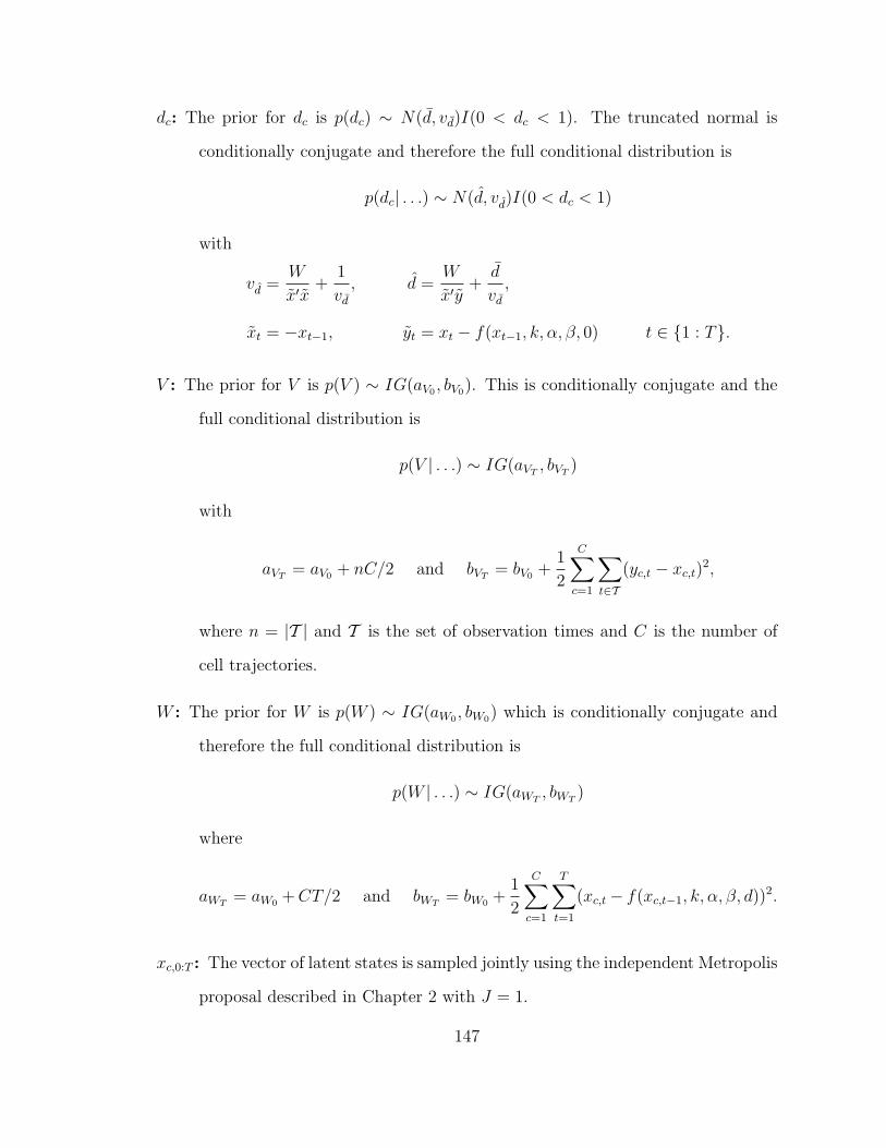
dc: The prior for dc is p(dc) ∼ N(d, vd)I(0 < dc < 1). The truncated normal is
conditionally conjugate and therefore the full conditional distribution is
p(dc| . . .) ∼ N(d, vd)I(0 < dc < 1)
with
vd =W
x′x+
1
vd, d =
W
x′y+d
vd,
xt = −xt−1, yt = xt − f(xt−1, k, α, β, 0) t ∈ 1 : T.
V : The prior for V is p(V ) ∼ IG(aV0 , bV0). This is conditionally conjugate and the
full conditional distribution is
p(V | . . .) ∼ IG(aVT, bVT
)
with
aVT= aV0 + nC/2 and bVT
= bV0 +1
2
C∑c=1
∑t∈T
(yc,t − xc,t)2,
where n = |T | and T is the set of observation times and C is the number of
cell trajectories.
W : The prior for W is p(W ) ∼ IG(aW0 , bW0) which is conditionally conjugate and
therefore the full conditional distribution is
p(W | . . .) ∼ IG(aWT, bWT
)
where
aWT= aW0 +CT/2 and bWT
= bW0 +1
2
C∑c=1
T∑t=1
(xc,t− f(xc,t−1, k, α, β, d))2.
xc,0:T : The vector of latent states is sampled jointly using the independent Metropolis
proposal described in Chapter 2 with J = 1.
147

C.2 Example motivated by pathway studies in systems biology
The details in this section are used in the analysis of Section 4.6 and model described
in equations (4.7). The fixed parameter set is θ = k, α, β, ψ, µ1:2, φ, V,W,U and the
latent states are x0:T and a0:T . The MCMC analysis was accomplished by sampling
each univariate fixed parameter followed by sampling the latent state. For each
unknown in the model, we outline the prior and full conditional distribution for that
parameter. In the following distributions, we use the notation fx(x, a, k, α, β, ψ) =
k+αa2x2
β+a2x2 + ψx and fa(a, µ, φ) = µ+ φ(a− µ) to represent the evolution functions for
the target and the activator, respectively. The data point yt is decomposed into two
components where y1,t and y2,t are the noisy measurement of at and xt, respectively.
k: The prior for k is p(k) ∼ N(k, vk)I(0 < k). The truncated normal is conditionally
conjugate and therefore the full conditional distribution
p(k| . . .) ∼ N(k, vk)I(0 < k)
where
vk =W
x′x+
1
vk, k =
W
x′y+k
vk,
xt =1
β + a2t−1x
2t−1
, yt = xt − fx(xt−1, at−1, 0, α, β, ψ) t ∈ 1 : T.
α: The prior for α is p(α) ∼ N(α, vα)I(0 < α). The truncated normal is condition-
ally conjugate and therefore the full conditional distribution
p(α| . . .) ∼ N(α, vα)I(0 < α)
where
vα =W
x′x+
1
vα, α =
W
x′y+α
vα,
xt =a2t−1x
2t−1
β + a2t−1x
2t−1
, yt = xt − fx(xt−1, at−1, k, 0, β, ψ) t ∈ 1 : T.
148

β: The prior for β is p(β) ∼ N(β, vβ)I(0 < βc). No conditionally conjugate prior
exists for β so a random walk Metropolis is used. A value is proposed from
β∗ ∼ N(β, σ2) and accepted with probability
ρ(β, β∗) = min
1,p(β∗)
p(β)
T∏t=1
N(xt|fx(xt−1, at−1, k, α, β∗, ψ),W )
N(xt|fx(xt−1, at−1, k, α, β, ψ),W )
.
ψ: The prior for ψ is p(ψ) ∼ N(ψ, vψ)I(0 < ψ < 1). The truncated normal is
conditionally conjugate and therefore the full conditional distribution is
p(ψ| . . .) ∼ N(ψ, vψ)I(0 < ψ < 1)
where
vψ =W
x′x+
1
vψ, ψ =
W
x′y+ψ
vψ,
xt = xt−1, yt = xt − f(xt−1, k, α, β, 0) t ∈ 1 : T.
µi: The prior for µi, i ∈ 0, 1 is p(µi) ∼ N(µi, vµi). The normal is conditionally
conjugate and therefore the full conditional distribution is
p(µi| . . .) ∼ N(µi, vµi)
where
vµi=
U
x′x+
1
vµi
, µi =U
x′y+µivµi
,
xt = 1− φ, yt = at − fa(at−1, 0, φ) t : ct = i.
φ: The prior for φ is p(φ) ∼ N(φ, vφ)I(0 < φ < 1). The truncated normal is
conditionally conjugate and therefore the full conditional distribution is
p(φ| . . .) ∼ N(φ, vφ)I(0 < φ < 1)
149

where
vφ =U
x′x+
1
vφ, φ =
U
x′y+φ
vφ,
xt = xt−1, yt = xt − fx(xt−1, at−1, k, α, β, 0) t ∈ 1 : T.
V : The prior for V is p(V ) ∼ IG(aV0 , bV0). Therefore the full conditional distribution
conditionally conjugate and is
p(V | . . .) ∼ IG(aVT, bVT
)
aVT= aV0 + T and bVT
= bV0 +1
2
T∑t=1
(y1,t − at)2 + (y2,t − xt)
2.
W : The prior for W is p(W ) ∼ IG(aW0 , bW0) which is conditionally conjugate and
therefore the full conditional distribution is
p(W | . . .) ∼ IG(aWT, bWT
)
where
aWT= aW0 + T/2 and bWT
= bW0 +1
2
T∑t=1
(xt − fx(xt−1, at−1, k, α, β, ψ))2.
U : The prior for U is p(U) ∼ IG(aU0 , bU0) which is conditionally conjugate and
therefore the full conditional distribution is
p(U | . . .) ∼ IG(aUT, bUT
)
.
aUT= aU0 + T/2 and bUT
= bU0 +1
2
T∑t=1
(at − fa(at−1, µ, φ))2.
x0:T : The vector of latent target states is sampled jointly using the independent
Metropolis proposal described in Chapter 2.
150
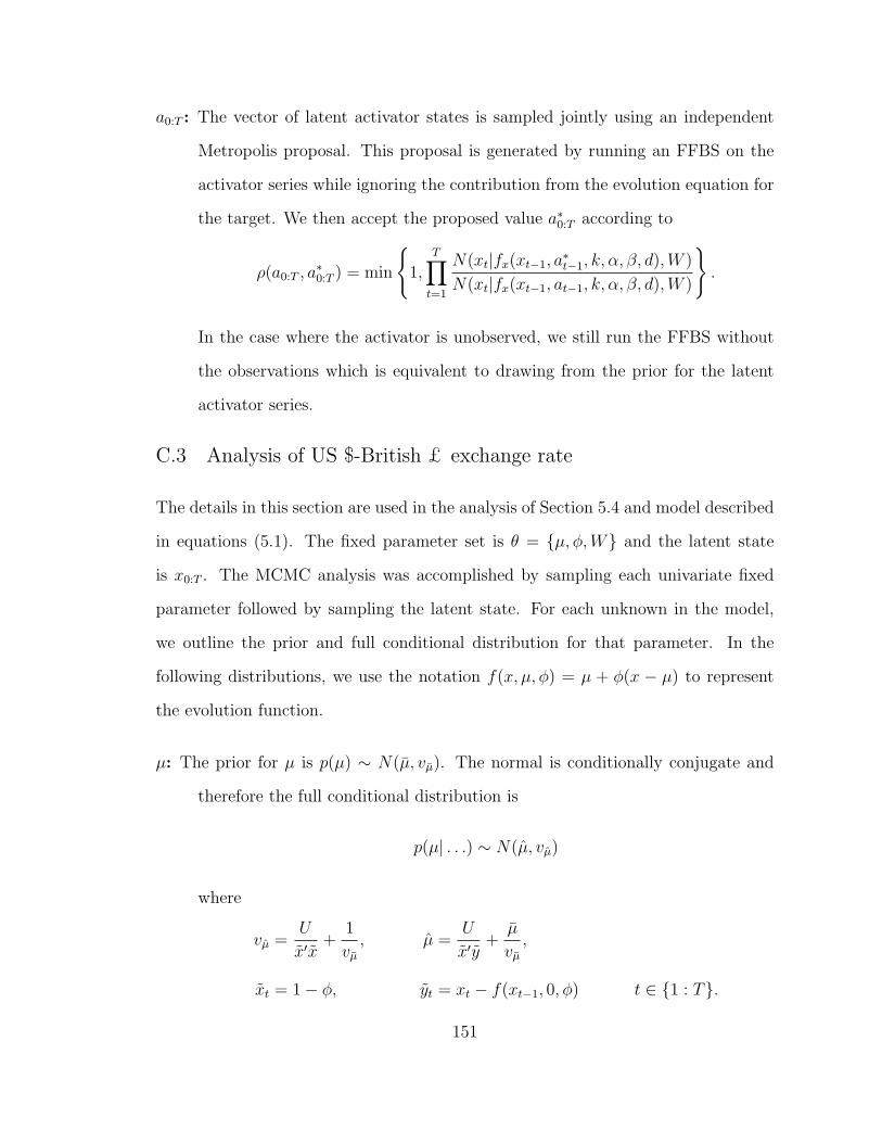
a0:T : The vector of latent activator states is sampled jointly using an independent
Metropolis proposal. This proposal is generated by running an FFBS on the
activator series while ignoring the contribution from the evolution equation for
the target. We then accept the proposed value a∗0:T according to
ρ(a0:T , a∗0:T ) = min
1,
T∏t=1
N(xt|fx(xt−1, a∗t−1, k, α, β, d),W )
N(xt|fx(xt−1, at−1, k, α, β, d),W )
.
In the case where the activator is unobserved, we still run the FFBS without
the observations which is equivalent to drawing from the prior for the latent
activator series.
C.3 Analysis of US $-British £ exchange rate
The details in this section are used in the analysis of Section 5.4 and model described
in equations (5.1). The fixed parameter set is θ = µ, φ,W and the latent state
is x0:T . The MCMC analysis was accomplished by sampling each univariate fixed
parameter followed by sampling the latent state. For each unknown in the model,
we outline the prior and full conditional distribution for that parameter. In the
following distributions, we use the notation f(x, µ, φ) = µ + φ(x − µ) to represent
the evolution function.
µ: The prior for µ is p(µ) ∼ N(µ, vµ). The normal is conditionally conjugate and
therefore the full conditional distribution is
p(µ| . . .) ∼ N(µ, vµ)
where
vµ =U
x′x+
1
vµ, µ =
U
x′y+µ
vµ,
xt = 1− φ, yt = xt − f(xt−1, 0, φ) t ∈ 1 : T.
151

φ: The prior for φ is p(φ) ∼ N(φ, vφ)I(0 < φ < 1). The truncated normal is condi-
tionally conjugate aside from the prior for x0 and therefore the full conditional
distribution is
p(φ| . . .) ∼ N(φ, vφ)I(0 < φ < 1)
where
vφ =W
x′x+
1
vφ, φ =
W
x′y+φ
vφ,
xt = xt−1, yt = xt − f(xt−1, µ, φ) t ∈ 1 : T.
W : The prior for W is p(W ) ∼ IG(aW0 , bW0) which is conditionally conjugate and
therefore the full conditional distribution is
p(W | . . .) ∼ IG(aWT, bWT
)
where
aWT= aW0 + T/2 and bWT
= bW0 +1
2
T∑t=1
(at − f(at−1, µ, φ))2.
x0:T : The vector of latent states is sampled jointly using the independent Metropolis
proposal described in Section 5.2.2.
C.4 Comparison of kernel smoothing with particle learning
The details in this section are used in the analysis of Section 6.2.3 and model de-
scribed in equations (6.2). The fixed parameter set is θ = (α, β, V,W ) and the latent
state is x0:T . The MCMC analysis was accomplished by sampling jointly from the
fixed parameters followed by sampling the latent state. Note that given the latent
state, the full conditional distribution for V is independent of the joint distribution
for (α, β,W ). Below we outline the prior and full conditional distribution in this
scheme.
152

V : The prior for V is p(V ) ∼ IG(aV0 , bV0) which is conditionally conjugate. There-
fore the full conditional distribution is
p(V | . . .) ∼ IG(aVT, bVT
)
where
aVT= aV0 + T/2 and bVT
= bV0 +1
2
T∑t=1
(y1,t − xt)2.
(α, β,W ): The prior for α, β, and W is a joint normal inverse-gamma which is con-
ditionally conjugate and therefore the full conditional distribution is available
and provided below (West and Harrison, 1997, see Ch. 17). For these results,
the notation y = (x1 x2 . . . xT )′, X = [(1 1 . . . 1)′ (x0 x1 . . . xT−1)′] is used.
p(W ) ∼ IG(aW0 , bW0), p(α, β|W ) ∼ N(c0,WC0),
p(W |x0:T ) ∼ IG(aWT, bWT
), p(α, β| . . .) ∼ N(cT ,WCT ),
aWT= aW0 + T/2, bWT
= bW0 + (y −XcT )′(y −XcT ) . . .
+ (cT − c0)′C−1
0 (cT − c0),
CT = (X ′X + C−10 )−1, cT = CT (X ′y + C−1
0 c0).
x0:T : The prior for x0 is normal and this is a linear Gaussian model so FFBS is used
to sample p(x0:T | . . .).
153

Appendix D
MATLAB code for algorithm implementation
This appendix contains many of the algorithms used throughout this thesis. In par-
ticular, it contains the algorithms to perform the methods described in Chapter 2
including mixture regeneration, the adaptive mixture filtering, backward sampling
from that filter, and calculation of the Metropolis-Hastings ratio. It also contains
the algorithms to perform the methods described in Chapter 5 including approxi-
mate updating of mixture components and adaptive mixture filtering for stochastic
volatility models.
154

D.1 Mixture regeneration
1 function [p m C] = regenerate(p1,m1,C1,J)2 %3 % [p m C] = regenerate(p1,m1,C1,J)4 %5 % This function will create a mixture of Gaussian approximation to6 % f(x) 6= \sum p1(i) N(m1(i),C1(i))7 % with the following properties:8 % * C will be equal and small9 % * m will be the J−quantiles of f()
10 % * p will be 1/J11
12 mn = p1'*m1; % Target mean13 vr = p1'*(C1 + (m1−mn).ˆ2); % Target variance14
15 if J==1, p=1;m=mn;C=vr; % If there is only one component16 else17 p = ones(J,1)/J; % Set all the components probabilities equal18 [mx ind] = max(p1); % Use for fzero starting value19 m = zeros(J,1); % Component means20
21 sd1 = sqrt(C1);22 % Set component means equal to density quantiles23 m(1) = fzero(@(x) 1/(1+J)−p1'*normcdf(x,m1,sd1),m1(ind),1/J/10);24 for j=2:J25 m(j)= myfzero(@(x) j/(1+J)−p1'*normcdf(x,m1,sd1),m(j−1));26 end27
28 % Set component variances equal and such that the mixture29 % variance is equal to the target variance30 C = repmat(vr − p'*(m−p'*m).ˆ2,J,1);31 end32
33 end
155

The myfzero function:
1 function RootMin = myfzero(Fun,X0)2 %3 % zero = myfzero(Fun,X0)4 %5 % This function finds a zero of Fun that is greater than X0.6 %7
8 RootMin = X0;9 while (Fun(RootMin)<0)
10 RootMin = RootMin−1;11 end12
13 RootMax = RootMin;14 while (Fun(RootMax)>0)15 RootMax = RootMax+1;16 end17
18 FMin = Fun(RootMin);19 FMax = Fun(RootMax);20 while (FMin−FMax>1e−8)21 RootMid = (RootMin+RootMax)/2;22 FMid = Fun(RootMid);23 if (sign(FMin)==sign(FMid))24 RootMin = RootMid;25 FMin = FMid;26 else27 RootMax = RootMid;28 FMax = FMid;29 end30 end31
32 end
156

D.2 Adaptive mixture filtering
1 function [p m C ap Rp G] = AM4(y,ff,df,fg,dg,V,W,p0,m0,C0,J)2 %3 % [p m C ap Rp G] = AM4(y,ff,df,fg,dg,V,W,p0,m0,C0,J)4 %5 % This function will perform the regenerating Gaussian sum filter6 % on the nonlinear Gaussian state space model:7 %8 % y t = ff(x t,t) + nu t nu t ¬ N[0,V t]9 % x t = fg(x t−1,t) + omega t omega t ¬ N[0,W t]
10 % x 0 ¬ sum j=1ˆJ p0(j) N(m0(j) ,C0(j) )11 %12 % Inputs:13 % y: Tx1 vector of observations14 % ff: observation function, ff(x t,t)15 % df: derivative of observation function16 % fg: evolution function, fg(x t−1,t)17 % dg: derivative of evolution18 % V: Tx1 vector of observation variances19 % (if V is a scalar, it is turned into a Tx1 vector)20 % W: Tx1 vector of evolution variances21 % (if W is a scalar, it is turned into a Tx1 vector)22 % p0: component probabilities for x 023 % m0: component means for x 024 % C0: component variances for x 025 % J: number of components26 %27 % Outputs:28 % p(t,j): probability of component j at time t29 % m(t,j): mean of component j at time t30 % C(t,j): variance of component j at time t31 % ap(t,j): prior mean of component j at time t (used in BS)32 % Rp(t,j): prior variance of component j at time t (used in BS)33
34 T = length(y);35 if length(V) == 1, V = V*ones(T,1); end36 if length(W) == 1, W = W*ones(T,1); end37 if size(p0,2) 6= 1, p0 = p0'; end38 if size(m0,2) 6= 1, m0 = m0'; end39 if size(C0,2) 6= 1, C0 = C0'; end40
41 m = zeros(T+1,J); C = m; p = m; logp = m; a = m; R = m;42 f = m; Q = m; e = m; A = m; F = m; G = m; ap = m; Rp = m;43
44 % Approximate the prior45 [tmp1 tmp2 tmp3] = regenerate(p0,m0,C0,J);46 p(1,:) = tmp1; m(1,:) = tmp2; C(1,:) = tmp3;
157

47
48 for t=1:T49 % waitbar(t/T,wb);50 for j=1:J51 ap(t+1,j) = fg(m(t,j),t);52 G(t+1,j) = dg(m(t,j),t);53 Rp(t+1,j) = G(t+1,j).ˆ2*C(t,j)+W(t);54 end55 % Regenerate56 [tmp1 tmp2 tmp3] = regenerate(p(t,:)',ap(t+1,:)',Rp(t+1,:)',J);57 p(t,:) = tmp1';58 a(t+1,:) = tmp2';59 R(t+1,:) = tmp3';60 logp(t,:) = log(p(t,:));61
62 if isnan(y(t))63 for j=1:J64 m(t+1,j) = a(t+1,j);65 C(t+1,j) = R(t+1,j);66 p(t+1,j) = p(t,j);67 logp(t+1,j) = logp(t,j);68 end69 else70 for j=1:J71 f(t+1,j) = ff(a(t+1,j),t);72 F(t+1,j) = df(a(t+1,j),t);73 Q(t+1,j) = F(t+1,j).ˆ2*R(t+1,j)+V(t);74 e(t+1,j) = y(t) − f(t+1,j);75 A(t+1,j) = R(t+1,j)*F(t+1,j)./Q(t+1,j);76 m(t+1,j) = a(t+1,j)+A(t+1,j)*e(t+1,j);77 C(t+1,j) = R(t+1,j)−A(t+1,j)*Q(t+1,j)*A(t+1,j);78 logp(t+1,j) = logp(t,j)−log(Q(t+1,j))/2−e(t+1,j)ˆ2/(2*Q(t+1,j));79 end80
81 % Adjust component probabilities to sum to 182 logp(t+1,:) = logp(t+1,:)−max(logp(t+1,:)); % avoid num. instab.83 tmp = exp(logp(t+1,:));84 p(t+1,:) = tmp/sum(tmp); logp(t+1,:) = log(p(t+1,:));85
86 % Regenerate87 [tmp1 tmp2 tmp3] = regenerate(p(t+1,:)',m(t+1,:)',C(t+1,:)',J);88 p(t+1,:) = tmp1;89 m(t+1,:) = tmp2;90 C(t+1,:) = tmp3;91 logp(t+1,:) = log(p(t+1,:));92 end % if isnan(y(t))93
94 end % end t95
96 end
158
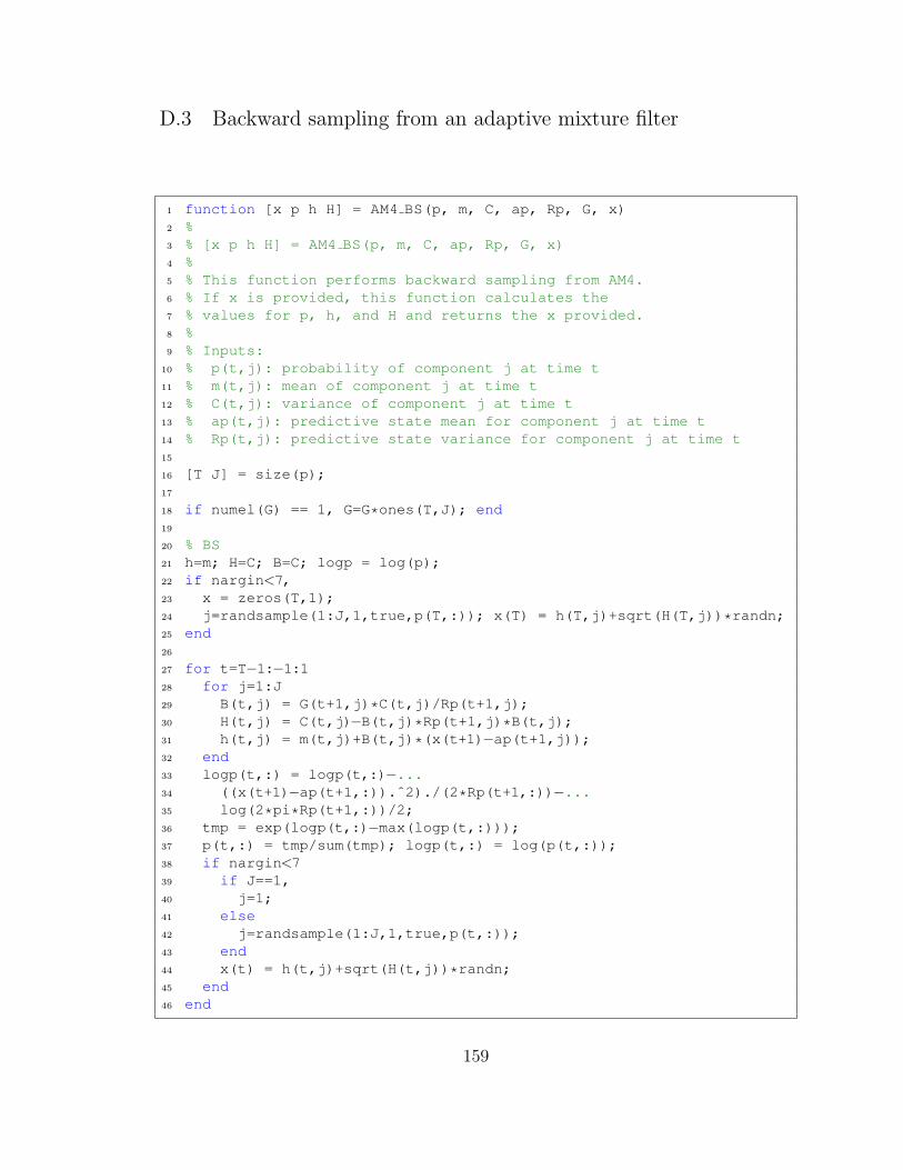
D.3 Backward sampling from an adaptive mixture filter
1 function [x p h H] = AM4 BS(p, m, C, ap, Rp, G, x)2 %3 % [x p h H] = AM4 BS(p, m, C, ap, Rp, G, x)4 %5 % This function performs backward sampling from AM4.6 % If x is provided, this function calculates the7 % values for p, h, and H and returns the x provided.8 %9 % Inputs:
10 % p(t,j): probability of component j at time t11 % m(t,j): mean of component j at time t12 % C(t,j): variance of component j at time t13 % ap(t,j): predictive state mean for component j at time t14 % Rp(t,j): predictive state variance for component j at time t15
16 [T J] = size(p);17
18 if numel(G) == 1, G=G*ones(T,J); end19
20 % BS21 h=m; H=C; B=C; logp = log(p);22 if nargin<7,23 x = zeros(T,1);24 j=randsample(1:J,1,true,p(T,:)); x(T) = h(T,j)+sqrt(H(T,j))*randn;25 end26
27 for t=T−1:−1:128 for j=1:J29 B(t,j) = G(t+1,j)*C(t,j)/Rp(t+1,j);30 H(t,j) = C(t,j)−B(t,j)*Rp(t+1,j)*B(t,j);31 h(t,j) = m(t,j)+B(t,j)*(x(t+1)−ap(t+1,j));32 end33 logp(t,:) = logp(t,:)−...34 ((x(t+1)−ap(t+1,:)).ˆ2)./(2*Rp(t+1,:))−...35 log(2*pi*Rp(t+1,:))/2;36 tmp = exp(logp(t,:)−max(logp(t,:)));37 p(t,:) = tmp/sum(tmp); logp(t,:) = log(p(t,:));38 if nargin<739 if J==1,40 j=1;41 else42 j=randsample(1:J,1,true,p(t,:));43 end44 x(t) = h(t,j)+sqrt(H(t,j))*randn;45 end46 end
159

D.4 Metropolis acceptance probability component calculation
1 function [logTar logPro] = ...2 AM4 Metropolis(y, x, ff, fg, V, W, m 0, C 0, p, h, H)3 %4 % [logTar logPro] = AM4 Metropolis(y,x,ff,fg,V,W,m 0,C 0,p,h,H)5 %6 % This function calculates the logarithm of the target distribution7 % and the logarithm of the proposal distribution when the components8 % for the proposal distribution are known. The target distribution is9 %
10 % y(t) = ff(x(t),t) + v(t) v(t) ¬ N(0,V)11 % x(t) = fg(x(t−1),t) + w(t) w(t) ¬ N(0,W)12 % x 0 ¬ N(m 0,C 0)13 %14 % The proposal distribution is defined at time t as15 %16 % x(t) ¬ sum j=1ˆJ p(t,j) N(h(t,j),H(t,j))17 %18 % p,h,H are associated with this x. If you need to calculate this for19 % a different x, use function AM4 BS with known x first.20 %21 % Inputs:22 % y(t): data at time t23 % x(t): latent state at time t24 % ff(x,t): observation function of x at time t25 % fg(x,t): evolution function of x at time t26 % V: observation variance27 % W: evolution variance28 % m 0: mean of x 029 % C 0: variance of x 030 % p(t,j): probability of component j at time t31 % h(t,j): mean of component j at time t32 % H(t,j): variance of component j at time t33 % Outputs:34 % logTar: log of the target distribution35 % logPro: log of the proposal distribution36
37 T = length(y);38 ObsTimes = find(¬isnan(y));39 nObs = length(ObsTimes);40 logp = log(p);41
42 % Evaluate the proposal43 logPro=0;44 for t=1:(T+1)45 tmp = −(x(t)−h(t,:)).ˆ2./(2*H(t,:))−log(2*pi*H(t,:))/2+logp(t,:);46 mx = max(tmp);
160

47 logPro = logPro+mx+log(sum(exp(tmp−mx)));48 end49
50 % Evaluate the target51 logTar = −nObs*log(2*pi*V)/2 ...52 −sum((y(ObsTimes)−ff(x(1+ObsTimes),ObsTimes)).ˆ2)/(2*V) ...53 −T*log(2*pi*W)/2−sum((x(2:end)−fg(x(1:end−1),(1:T)')).ˆ2)/(2*W) ...54 −log(2*pi*C 0)/2−sum((x(1)−m 0)ˆ2)/(2*C 0);55
56 end
161

D.5 Approximate updating of mixture components
1 function [p m C] = ...2 ApproximateMixtureUpdating(y,q,a,R,LogProbDensFunc,d1,d2)3 %4 % [p m C] = ApproximateMixtureUpdating(q,a,R,LogProbDensFunc,d1,d2)5 %6 % This function will approximately update a mixture prior under the7 % observation model p(y |x) = ProbDensFunc(y,x).8 %9 % Input:
10 % y: observation11 % q: vector of prior components probabilities12 % a: vector of prior components means13 % R: vector of prior component variances14 % LogProbDensFunc(y,x): a function to evaluate log p(y |x)15 % d1(y,a): −(d/dx) LogProbDensFunc(y,x) evaluated at x=a16 % d2(y,a): −(dˆ2/dxˆ2) LogProbDensFunc(y,x) evaluated at x=a17 %18 % Output:19 % p: vector of posterior component probabilities20 % m: vector of posterior component means21 % C: vector of posterior components variances22
23 if size(q,2) 6= 1, q=q'; end24 if size(a,2) 6= 1, a=a'; end25 if size(R,2) 6= 1, R=R'; end26
27 J = size(q,1); % number of mixture components28 logq = log(q); % for use in updating mixture component weights29
30 d1a = d1(y,a);31 d2a = d2(y,a);32 d1aoverd2a = d1a./d2a; % pre−computed for speed33 overd2a = 1./d2a; % pre−computed for speed34
35 % Calculate posterior component variance36 C = 1./(d2a+1./R);37
38 % Calculate posterior component mean39 m = C.*(d2a.*(a−d1aoverd2a)+a./R);40
41 % Calculate (proportional to) posterior component log probability42 logp = logq...43 +LogProbDensFunc(y,a)...44 +LogGaussPDF(d1aoverd2a,0,sqrt(overd2a+R))...45 −LogGaussPDF(d1aoverd2a,0,sqrt(overd2a));46
162

47 % Renormalize component probabilities48 logp = logp−max(logp);49 p = exp(logp);50 p = p./sum(p);51
52 end
163

D.6 AM4 for stochastic volatility model
1 function [p m C ap Rp] = AM4 SV(y,mu,phi,W,m0,C0,J)2 %3 % [p m C ap Rp] = AM4 SV(y,mu,phi,W,m0,C0,J)4 %5 % This function will perform AM4 on the6 % approximate stochastic volatility model:7 %8 % y t = x t + nu t nu t ¬ log−chi 1ˆ2/29 % x t = mu+phi (x t−1−mu) + omega t omega t ¬ N[0,W]
10 % x 0 ¬ N(m0 ,C0 )11 %12 % Inputs:13 % y: Tx1 vector of observations14 % mu: mean of AR process15 % phi: AR parameter16 % W: Tx1 vector of evolution variances17 % (if W is a scalar, it is turned into a Tx1 vector)18 % m0: mean for x 019 % C0: variance for x 020 % J: number of components21 %22 % Outputs:23 % p(t,j): probability of component j at time t24 % m(t,j): mean of component j at time t25 % C(t,j): variance of component j at time t26 % ap(t,j): prior mean of component j at time t (used in BS)27 % Rp(t,j): prior variance of component j at time t (used in BS)28
29 y = [NaN; y];30 T = length(y);31
32 LogProbDensFunc = @(y,x) −log(pi/2)/2+y−x−.5*exp(2*(y−x));33 d1 = @(y,a) 1−exp(2*(y−a));34 d2 = @(y,a) 2*exp(2*(y−a));35
36 m = NaN*zeros(T,J);37 C = NaN*zeros(T,J);38 p = NaN*zeros(T,J);39 a = NaN*zeros(T,J);40 R = NaN*zeros(T,J);41 ap = NaN*zeros(T,J);42 Rp = NaN*zeros(T,J);43
44 % Approximate the prior45 [tmp1 tmp2 tmp3] = regenerate(1,m0,C0,J);46 p(1,:) = tmp1; m(1,:) = tmp2; C(1,:) = tmp3;
164

47
48 for t=2:T49 for j=1:J50 ap(t,j) = mu+phi*(m(t−1,j)−mu);51 Rp(t,j) = phiˆ2*C(t−1,j)+W;52 end53
54 a(t,:) = ap(t,:);55 R(t,:) = Rp(t,:);56 p(t,:) = p(t−1,:);57
58 if isnan(y(t))59 m(t,:) = a(t,:);60 C(t,:) = R(t,:);61 else62 [tmpp tmpm tmpC] = ...63 ApproximateMixtureUpdating(y(t),p(t,:),a(t,:),R(t,:), ...64 LogProbDensFunc,d1,d2);65
66 % Regenerate67 if J>1, [tmpp tmpm tmpC] = regenerate(tmpp,tmpm,tmpC,J); end68 p(t,:) = tmpp; m(t,:) = tmpm; C(t,:) = tmpC;69 end % end isnan(y(t))70 end % end t71
72 end
165

Appendix E
Image segmentation and dynamic lineage analysisin single-cell fluorescence microscopy
The paper on the following pages will be published in Synthetic Biology, 2009 (Wang
et al., 2009).
166

Image segmentation and dynamic lineage analysis in single-cell fluorescence microscopy Quanli Wang1,2, Jarad Niemi1, Chee-Meng Tan3, Lingchong You2,3 and Mike West1,2
1Department of Statistical Science, Duke University 2Institute for Genome Sciences & Policy, Duke University
3Department of Biomedical Engineering, Duke University
Abstract An increasingly common component of studies in synthetic and systems biology is analysis of dynamics of gene expression at the single-cell level, a context that is heavily dependent on the use of time-lapse movies. Extracting quantitative data on the single-cell temporal dynamics from such movies remains a major challenge. Here, we describe novel methods for automating key steps in the analysis of single-cell, fluorescent images – segmentation and lineage reconstruction – to recognize and track individual cells over time. The automated analysis iteratively combines a set of extended morphological methods for segmentation, and uses a neighborhood-based scoring method for frame-to-frame lineage linking. Our studies with bacteria, budding yeast and human cells, demonstrate the portability and usability of these methods, whether using phase, bright field or fluorescent images. These examples also demonstrate the utility of our integrated approach in facilitating analyses of engineered and natural cellular networks in diverse settings. The automated methods are implemented in freely available, open-source software.
167

INTRODUCTION Time-lapse microscopy technologies now enable detailed data generation on dynamic cellular processes at the single cell level (1, 2). Recent studies have highlighted the use and importance of this technology for investigating biological noise in the dynamics of gene regulation, competence pathways in Bacilus subtili, and aspects of cell growth and proliferation, among other areas (2,3,4,5,6,7). Mathematical and statistical models are of growing interest in describing and testing hypothesis for such systems (9,10,11), and rely on extraction of data from time-lapse microscopy imaging techniques that generate sequences of individual, pixel-based image frames. Unlike data generated from flow cytometry, which represent snapshots of cellular states, time-lapse movies with sufficiently high temporal and spatial resolution allow time courses of gene expression dynamics to be established at the single-cell level. These time courses are critically important in studies investigating the dynamics of both natural (12,13,14,15) and synthetic (16,17,18,19) cellular networks, dynamics that are often masked at the population level. However, recognizing cells as objects in images, and tracking them from one image to the next, remain as central technical challenges (1). These tasks, segmentation and tracking, respectively, can be approached either manually or automatically. Typically, humans are good at these tasks, but automation – essential for this fast-developing technology – is difficult and poses open questions for methodology development. Depending on the cells being segmented and tracked, various existing algorithms are available (20,21,22,23,24). A universal solution to cell segmentation and tracking, applicable across cell types, has yet to be described. Algorithms that work well on one set of images often perform poorly on another set due to differences in the features that are exploited. A major goal in algorithm design and software development is then to provide a set of tools capable of extracting cell-like objects from many different types of images. Attempts have been made in both commercial and public domain software packages to solve these issues. Commercial software, including Imaris from BitPlabe, Amira from Mercury Computer Systems, Volocity from Improvision, MetaMorph from Molecular Devices and Matlab Image Processing toolbox from MathWorks, are mainly for general purpose image analysis, not specific nor customized to microscopy images. Among public-domain tools in development, Image-J is a general purpose image analysis program, while CellProfiler (23), Cell-ID (20), CellTracker (24), and GoFigure(1) aim to address segmentation and/or tracking in more specific areas. For example, Cell-ID was developed for automatic segmentation, tracking, and quantification of fluorescence protein levels in yeast. For specific synthetic or natural biological systems, ad hoc algorithms have also been adopted for analyses of gene expression dynamics in bacteria (5), yeast (25), and mammalian cells (26). The algorithms implemented in above-mentioned tools use a number of variations of watershed and level-set approaches for segmentation. The success of these approaches depends largely on success in defining initial cell identity and location markers. When cells are tightly clustered, as is often the case with data on E. coli and yeast, for example, it is typically difficult to correctly identify initial cell objects to avoid mis-segmentation. Also, the methods used to define cell markers vary with cell type and
168

image type, thus reducing algorithm portability. To address these questions, we develop the concept of hybrid grey-scale/black-white images and extend existing image filters and mathematical morphological operators for grey-scale images to work with these hybrid images. This approach allows us to extract cells from an image in an iterative process that gradually converts the grey-scale image into a black-white mask thus segmenting the image into cells, without relying on initial cell markers. Moreover, tracking algorithms used in existing tools also face portability challenges: they often accomplish the tracking task by minimizing ad hoc global energy functions that are problem-specific, and typically do not consider locally clustered cells. To overcome these complications, we incorporate neighboring cell information to compute numerical likelihood scores for cell identity between each pair of time steps t to t+1. We then apply an integer programming method to generate frame-to-frame correspondences between cells and the lineage map. The resulting, fully automated analysis, wrapped in an open-source Matlab application, is demonstrated here on two E. coli bacteria data sets, one yeast dataset and one human cell data set. Full algorithmic, workflow and analysis details, and more extensive examples, are given in several sections of the Supplementary Materials. Additional information and examples, together with the source code, a graphical user interface, examples of alternative workflows and other supporting documents, can be found at the CellTracer website (http://www.stat.duke.edu/research/software/west/celltracer/). With this methodology and tool, we have been able to successfully analyze single-cell time-lapse movies of cellular dynamics for diverse cell types, spanning from bacteria to yeast to human cells and diverse image types, from phase to bright-field to fluorescence images. As such, we believe it will facilitate quantitative spatiotemporal analysis of synthetic and natural cellular networks. RESULTS Image preprocessing and hybrid filters on hybrid grey-scale/black-white image Preprocessing begins with a three-step partition of an initial grey-scale image into three distinctive regions: background, border, and undecided. The first step identifies the background using a modified nonlinear range filter followed by a standard morphological dilation. This recognizes regions that do not vary much and yet are large enough to be part of a cell. The second step identifies border regions that are not background or part of a cell, using an extended high-pass filter that operates on the masked image from the first step. Undecided regions are regions yet to be classified. It is also sometimes useful to re-label undecided pixels with extreme values as border regions by global thresholding. Recognizing that bacterial, yeast and human cells typically have smooth borders, we used a nonlinear range filter with a disk-shaped neighborhood, or a structure element. The disk size has to be larger than the maximum width of cells from all images. Once these range values are calculated, a threshold is chosen such that a pixel with range value less than the threshold will be labeled as 0, an indicator for background. The
169

resulting images are grey-scale with zero values indicating background. If we also assign special meaning to the largest values in the grey-scale image (255 for 8-bit images), as we do (below) for cell borders, we create a hybrid grey-scale/black-white image. In contrast, most other filters will end up with either black-white or grey-scale images only. Consequently, we also have to modify the usual high-pass filter not to use the pixels that take zero values when identifying the border regions in the initial partition. This can be done with a masked neighborhood approach. That is, we exclude all pixels that are masked to be the black-white during filtering, and use only pixels in a neighborhood that are part of the grey-scale image. This mask-based strategy, including the modified range-filter in the previous step, can be applied to other filters (Supplementary Note 2). In general, we can extend the above ideas to design a class of mask-based filters on hybrid images, as follows. Let ),( MIH = be a hybrid image comprised of a grey-scale image I and a black-white mask M. Let )(' HFH = be a function where the output
)','(' MIH = is also a hybrid image, created via ( ', ') ' ( ) ( , ).I M H F H F I M= = = (1) Then F is called a hybrid filter if ),*.(),( MMIFMIF = (2) for all I and M, where.* represents the element-wise product. In other words, 'H only depends on pixel intensity values in I that have corresponding non-zero values in M. With this notation, given any hybrid image ( , ),H I M= we formally define a specific class of hybrid filters, called hybrid range filters (or HRFs), as follows. Each HRF is defined by a specified range parameter 0.r > For each image pixel ( , ),i j denote by
,i jE the structure element centered at the pixel, and define , ,( )i j i jU I E M= ∩ where ∩ is the set intersection operator. Then the HRF map ( ', ') ( , )I M F I M= is given by
⎪⎩
⎪⎨
⎧ ≤−=
,),0,0(
,)min()max(),1,()','(
,,,
,,
otherwise
rUUifIMI
jijiji
jiji (3)
Hence, to calculate the output gray-scale intensity value ', jiI , the HRF first extracts all the pixels from its neighborhood as defined by the structure element, and then these pixels are further selected according to the corresponding binary mask. The output intensity is then kept the same as input only when the intensity values from the above selected neighborhood fall into the range defined by .r The output binary mask ', jiM is simply set to 1 when the corresponding grey-scale intensity is non-zero. In addition to range filters, we can design hybrid median, mean, or rank filters, in an obvious extension of the above definition of range filters. There are several advantages to these hybrid filters. First, both black-white and grey-scale images can be treated as special cases of the hybrid images by using proper masks, thus avoiding the need to
170

distinguish the types of input images. For a pure grey-scale image, the mask M is a matrix of ones and for a pure black-white image M is a zero matrix of the same size as I. Second, as the input and the output images are always of the same type, we can combine various types of filters sequentially to address different filtering needs. Third, instead of being forced to threshold the grey-scale image into black-white at some point of the image processing all at once, we can gradually threshold the image in an iterative and selective way and slowly turn an input grey-scale image to an output black-white image. This advantage will be demonstrated in the segmentation step below. Figure 1 gives an example of applying hybrid filters to preprocess a raw, grey-scale image. This process generates a hybrid image by classifying some pixels as background and others as cell borders while keeping remaining regions for further segmentation. Figure 1a shows three images of engineered E. coli bacteria programmed via a synthetic gene circuit (Supplementary Note 1). The cells are generally represented by darker pixels and surrounded by bright borders while the grey regions are background. Figure 1b is the result of applying the hybrid range filter to identify background as colored in green. Figure 1c is the result of applying the hybrid high-pass range filter to Figure 1b to identify border regions, colored in blue. Figure 1d is the result of further applying a global threshold filter to mark more pixels as borders. Note that this preprocessing just gives an initial partition for the input images, and may or may not be needed for every data set analysis. Segmentation with iterative/selective masked erosion and dilatation Segmentation identifies groups of pixels as cell objects. A common challenge with any algorithm is over- or under- segmentation (27,28,29). We approach this issue using an iterative algorithm that couples our hybrid filters with hybrid smoothing and dilation. We extend the concept of hybrid filtering to image smoothing and erosion/dilation (Supplementary Note 2). The hybrid image from the preprocessing step is input to analysis that applies a hybrid filter, or a combination of filters, to erode the undecided regions, followed by hybrid dilation and smoothing to restore most of the pixel values changed by the filter. The overall result is a subtle change in the mask associated with the hybrid image. We iteratively repeat this process, possibly with slightly more aggressive parameter settings, to gradually change the associated mask until a stopping rule is met (Supplementary Note 4). This final mask associated with the hybrid image is the resulting segmented image. We enhance the above strategy by adding a cell object modeling and selection step at the end of each iteration. Recognizing that cells have common morphological features (shape, size, smoothness) we define cell or object shape models. Disconnected segmented regions – referred to as blobs – in the binary mask are labeled, evaluated, scored and then classified into two groups based on the object shape model. Here we apply this method to set of data generated with engineered E. coli carrying a population control circuit (31) (Supplementary Note 1). This data set is challenging in that many bacteria are elongated due to the circuit function and that there is great diversity in the sizes of closely clustered individual bacteria. With E. coli data, the cell object model assumes a straight or curved cigar shape and a minimum pixel volume; in the example of Figure 1, all blobs are classified as either cells or undecided. Undecided blobs are
171

subject to further segmentation and cells are considered done with no further segmentation performed. This approach proves to be very useful especially when the cells exhibit diversity in scale, e.g., cells differing in diameter, in which case cells at different scales will be picked up at different iterations. More details appear in the Methods section and Supplementary Note 4. We illustrate this approach in Figure 2 for the dataset used in the preprocessing step above. Figure 2a shows the result of using a hybrid rank filter with disk-shape structure element to the hybrid images in Figure 1d. Figure 2b shows the hybrid image after further smoothing, thickening, and re-smoothing to Figure 2a. Many larger blobs in Figure 1d are broken down into smaller blobs. By thresholding, all blobs in Figure 2b are classified into two subsets as shown in Figure 2c and Figure 2d. Figure 2c shows the binary masks of the blobs with lower scores that will not be further segmented and Figure 2d shows the blobs with higher scores and will be subject to further segmentation. Figure 2e is the final segmentation (cell coloring is arbitrary and only for visuals). The same approach for yeast and human cells uses a slightly different cell object shape model. The main difference is that we assume cells have convex or nearly convex shapes, instead of the “bendy” cigar shape. Detailed description of this model can be found in Supplementary Note 6. Though designed for yeast and human cells, this model works equally well on bacterial examples, illustrating the robustness of the method. Once the iterations terminate, cells are labeled by recognizing disconnected blobs in the binary mask image. Basic quantities such as shape, size, boundary, and centroid can then be measured using techniques such as described in (20). Cell lineage reconstruction through neighborhood-based scoring Segmentation generates a sequence of images with objects segmented in each. To track cells over time and to reconstruct lineage trees, we use a two-step algorithm to first construct score matrices for all cells in each pair of consecutive images and then apply an optimization algorithm to obtain the frame-to-frame correspondence matrices. Suppose that image t has m cells and image t+1 has n cells. A forward score matrix (m by n) and backward score matrix (n by m) describe the likelihood of a cell in image t corresponding to a cell in image t+1 and that of a cell in image t+1 corresponding to a cell in image t, respectively. These matrices are further combined and transformed into a 0-1 correspondence matrix with 1 indicating a correspondence between a cell in image t and a cell in image t+1. Due to cell growth, death, or division, a cell in image t can correspond to 0, 1 or 2 cells in image t+1. To construct forward and backward scores for each pair of cells, we calculate geometric overlapping scores for the pair. We then locate all neighbors of each cell in each image and compute a pair of neighborhood scores over the neighborhood of each cell using the overlapping scores. By repeatedly shifting one image slightly, we recalculate overlapping and neighborhood scores for cell pairs and record the final scores as the largest combined neighborhood score over all shifts within a predefined distance. We make these scores more robust by using a threshold when calculating the neighborhood
172

scores so that small overlapping scores are not used to calculate final scores. Note that we do not specify a cell object model for the tracking algorithm. Instead, only the area representing a cell is used in the algorithm. By design, this neighborhood-based approach introduces robustness to image shifting during image capturing or cell movement. Figure 3 provides an example for calculating the score for a pair of E. coli cells, using data of Rosenfeld et al. (4). Figures 3a and 3b show two images at consecutive times with the pair of cells labeled in blue. Figure 3c is the result if we overlay the segmented images. This will not yield an acceptable score as two highlighted cells do not overlap at all. Instead, to construct a pair of scores for the cell at these two times, the neighborhoods for these cells are first located as shown in Figure 3d and 3e respectively. Then by shifting image 3b around, the best scores are obtained at the overlapping position as shown in Figure 3f. The bright yellow indicates the cells used to construct the scores. To transform the forward and backward score matrices into a single correspondence matrix, we start by noting that a cell in image t can disappear (die), grow, or divide into two cells in image t+1. So a cell in image t can only correspond to 0, 1, or 2 cells in image t+1. We also assume that a cell in image t+1 can correspond to at most 0 or 1 cells in image t, which restates the fact that a cell is an orphan or a descendent of a cell in image t. We then combine the two score matrices using dot product and calculate the row and column maxima in the combined score matrix; our algorithm then scans the combined score matrix to locate values that are both row and column maxima and assigns matches for corresponding cell pairs. During this process, if more than two cells in image t+1 can be assigned to one cell in image t the backward score matrix is referenced so that the two cells with best scores are used to assign the matches. We repeat this process while excluding the cells in image t+1 that are already matched and enforcing the cell growth event restraints until no more correspondences can be found. Once the correspondence matrices for all consecutive images are generated, we reconstruct the cell lineage trees by linking the sequence of correspondence matrices. Individual tracks can be further obtained by back-tracking the cells identified in the last frame to the cells in the first frame from the lineage trees. Figure 4a shows the combined score matrix for Figure 3, displayed as a heat map. Figure 4b shows the resulting correspondence matrix heat map after applying our optimization algorithm. This can be converted into a 0-1 correspondence matrix by identifying those scores above a specified threshold. From the image, we notice from the columns that each cell corresponds to only one cell from the previous image; similarly, from the rows we see that each cell corresponds to one or two cells (cell splitting) in the following image. Figure 4c shows a complete lineage tree for cell 1 in images 1 through 25 (displayed using GraphExplore: www.stat.duke.edu/research/software/west/graphexplore.html). The numbers in each node represent the image index and the cell index, respectively. Comparison with existing algorithms Sigal et al. (26), Gordon et al. (20), and Charvin et al. (30) demonstrated segmentation/tracking results on human and yeast cells using the Cell-ID, CellProfiler
173

and other tools. While complete yeast segmentation/tracking results are not available from (20), Figure 5a provides the correspondence heat map analogous to Figure 4a using the methods in (20). Compared to Figure 4a, it shows more small but non-zero values (in light blue) and fewer large values (in bright red). It is evident that our neighborhood score based tracking method provides a much sharper score matrix with substantially improved cell correspondences as indicated by red/orange pixels. The Sigal et al. study provided human cell imaging data in terms of supplementary movies as well as summaries of cell tracking results. This human data example provides a nice context for a side-by-side comparison with our method. Figure 5b demonstrates all 97 tracks reconstructed using our approach as compared with only 57 reported in (26). Further investigation based on our full tracking result suggests that there are at most 99 actual tracks from the last frame back to the first frame in the movie. i.e., our algorithm reconstructs almost 98% of actual tracks in the movie. Importantly, our analysis was a direct application of the automated method applied to bacterial data with no additional parameter tuning. More details on analysis of this data set, as well as additional examples using budding yeast data, can be found in Supplementary Note 6. DISCUSSION Our results demonstrate the utility and portability of our cell segmentation and tracking analysis for single-cell images of bacterial, yeast and human cells. The method applies similarly to other cell types using cell object shape models. Whatever the cell type, the automated, iterative algorithm for segmentation provides a novel and accurate way to extract cell information from time-course images. The concept of hybrid images and hybrid image based filters can be readily ported to existing tools that are designed purely for grey scale or black-white images. The neighborhood-based score function provides an efficient way to track cells through time. By using very common cell features and avoiding modeling cell growth transformations, our approach is robust and has good portability for deployment in other studies. By thresholding and using only higher scores when calculating correspondence, we can easily make the tracking algorithm iterative to deal more complicated cases and design algorithms that allowing skipping a frame for cell correspondence. Common methods such as background filtering, contrast enhancement, iterative morphological operations are of proven utility in image segmentation. However, effectively combining such methods, as several prior studies have done, is challenging as these operators each apply to the entire image under investigation without discrimination and thus often create undesired side effects. Our hybrid image-based operators allow us to take advantage of these useful methods but in such a way as to minimize these undesired side effects. Depending on the types of images to be analyzed, the image preprocessing step can be vital to the success of segmentation. In the contexts here, image preprocessing is tuned to work specifically with cells that have smooth shapes and that are generally represented by pixels that are darker or brighter than the surrounding environment, which for example, might not be the case for DIC images. However, the general strategy
174

can be ported to deal with other cell types based on alternative assumptions about distinctive border and inner regions. Our iterative approach for cell segmentation gives another example of deploying different operators defined on hybrid images to selectively target the unclassified regions of images while leaving well classified regions untouched. This approach is especially useful when the cells in the images have different scales or distinctive subclass features. Compared to commonly used global and adaptive threshold methods, iterative morphological erosion/dilation, or watershed based methods for segmentation, our analysis across a range of examples is uniformly effective in terms of overcoming the common pitfalls of over- or under- segmentation. A core issue of cell tracking is to determine the correspondences between cells in two consecutive images. Some assumptions have to be made about the image acquisition rate and also about the cell growth rate to have a well defined problem. Low image sampling rate, high cell growth rate, or both will make tracking nearly impossible without strong assumptions. Even for well-behaved data, however, finding correspondences between cells across images is an NP-complete problem. This problem is further complicated by poor segmentation and various transformations and spatial mappings due to cell growth such as change of shapes, cell division and also imperfect image acquisition techniques. Some of the best methods currently available use joint estimation of correspondence and spatial mappings via optimization of energy functions (32). The success of such approaches is heavily dependent on the design of energy function and the choice of optimization technique as well as the choice of mapping functions and cell features. Other approaches use more formal statistical models to estimate the likelihoods of cell death and division between frames and consolidate these likelihood values into correspondence using integer programming optimizations (33). Our approach has built on the best characteristics of these general strategies. We first derive a score that uses only one robust feature extracted from cells together with the neighborhood information. Then our greedy search algorithm consolidates the scores into cell correspondences. To construct the score, we intentionally avoid using the popular cell feature candidates such as volume, orientation, centroid, and major and minor axis. Instead, we used geometric overlapping as a basis for our score. However, some obstacles have to be overcome to use this feature successfully. First, the standard overlapping measure is symmetric for two involved images and does not deal with cell division events correctly. We address this issue by using forward and backward overlapping measures, which turns out to be critical for successful tracking of budding yeast cells. Second, systematic shifts of image or local movements of cells can cause standard overlapping measure to be unstable. We address this issue by shifting one image around and finding the best local neighborhood match before deciding the actual overlapping measure. The resulting overlapping measure is robust to these obstacles and can be easily applied to other cell images. As a result, there is very little parameter tuning for three different types of cells we analyzed here. To further test our tracking algorithm, we have rerun analyses by skipping every other frame in the image sequences and have found that there is little change in tracking results for E. coli and human cells. In the case of budding yeast cells, however, we did observe more tracking mistakes at times when daughter cells were just separated from mother cells.
175
METHODS Initial partition to convert grey-scale image into hybrid image The input grey-scale phase images are first preprocessed to generate hybrid images for further segmentation. To identify the initial background, we customized the range filter from the Matlab image processing toolbox to use a disk shaped structure element in observing the fact that all the cells under consideration have rather smooth shapes. We then scan all image frames to generate an initial estimate of the maximum half width, r, of all cells and choose the radius of the disk structure element to be between r and 2r. After applying the range filter, a fixed threshold is chosen so that in any image, a pixel with range value less than the threshold will be marked as 0 for background. While there might be optimal values for such parameters to get best initial background partition, we find this usually gave satisfying initial results after a few preprocessing attempts. The resulting hybrid images are then fed into a modified high-pass range filter to identify the cell border regions. The high-pass range filter is modified in two ways: we use the disk shaped structure element as we did for background, and we exclude all background pixels when recording the minimum value within the neighborhood of each pixel. We choose a value for this threshold so that only the very obvious border pixels are marked as 255 for border in our 8-bit input images. Iterative cell segmentation Iterative cell segmentation in general involves the following steps: (1) Label disconnected blobs in the associated binary masks from hybrid images. (2) Filter each labeled blob using hybrid filters to obtain a refined estimate, which usually will break down some undesired blobs into smaller blobs. (3) Score the refined blobs based on the cell shape model assumptions. Some example cell shape models can be found in Supplementary Notes 3 and 6. (4) Threshold all blobs into two subsets using a user chosen score threshold. (5) Keep the subset of blobs with lower scores unchanged and repeat (1) through (4) until no more blobs can be broken down and the resulting binary mask is taken as the segmentation result. For our example datasets, step (2) is further detailed as follows: (2a) For each blob in the subset with higher scores, a modified rank filter with disk-shape structure element is applied to the corresponding grey-scale blob to identify the pixels with higher intensity values and to erode them from the corresponding binary mask; (2b) The eroded mask blob is then further smoothed by applying a distance transform to the inverted mask,which caculates the distance between each pixel that is set to zero and the nearest nonzero pixel in the mask, and then thresholding it; (2c) The smoothed mask is dilated through a morphological thickening with respect to the original binary mask in (2a). As a result of (2a) through (2c), many blobs with higher scores will break down into smaller blobs and yield further segmented hybrid images. We have also developed alternative procedures in the software for step 2 that user might find more effective for specific dataset or cell types. Construction of forward and backward score matrices
176

We use the strategy described earlier to construct the forward and backward score matrices. Our realization of this strategy uses the following implementations. At time t, we define the forward geometric overlapping score for cell i in image t and cell j in image t+1 as the ratio of number of pixels in cell i divided by the total number of pixels in both cell i and cell j. Similarly, we define the backward geometric overlapping score for cell j in image t+1 and cell i in image t as the ratio of number of pixels in cell j divided by the total number of pixels in both cell i and cell j. We regard a cell i is in the neighborhood of a cell j if they overlap at least once if we shift cell i within given pixels p, where p controls the maximum neighborhood size. The threshold we chose to decide if a geometric overlapping score will be counted as valid is 0.2. This threshold can be set to a higher value if cells do not move or change shape a lot. The combined neighborhood score is the square of the sum of the forward and backward scores. Correspondence matrix We transform the score matrices into correspondence matrix using the greedy approximation algorithm implemented in CellTracer, with implementation details provided in Supplementary Note 5. Alternative implementations We have presented one particular implementation of our overall strategy and resulting algorithm, in a form that works well on all three types of testing data sets – bacterial, yeast and mammalian cells – and based on phase, bright field or fluorescent images. It is however understood that improved segmentation results, or more efficient algorithms, may be achieved by tailoring the workflow to more specific features of a data set. Our emphasis is on robustness and portability, but we have detailed the opportunities to further customize the approach, if desired, in supporting material and describe some such customization in explicit detail in examples at the software website. ACKNOWLEDGEMENTS We are grateful to the editor and anonymous referees for constructive comments; to M. Elowitz and N. Rosenfeld for discussion and provision of a data set (Figure 3, Supp. Note 2); to Philippe Marguet for a data set (Supp. Note 4); and to Eric Siggia for a yeast data set (Supp Note 6). Research was partially supported by the National Science Foundation (DMS-0342172, BES- 0625213) and National Institutes of Health (NCI U54-CA-112952). Any opinions, findings and conclusions or recommendations expressed in this work are those of the authors and do not necessarily reflect the views of the NSF or NIH.
177

REFERENCES 1. Megason, S. G. & Fraser, S.E. Imaging in Systems Biology. Cell 130, 784-795 (2007). 2. Longo, D. & Hasty, J. Dynamics of single-cell gene expression. Molecular Systems Biology, 2:64 (2006) 3. Elowitz, M.B., Levine, A.J., Siggia, E.D. & Swain, P.S. Stochastic gene expression on a single cell. Science 297, 1183-1186 (2002). 4. Raser, J.M. & O’Shea, E.K. Control of stochasticity in eukaryotic gene expression. Science 304, 1811-1814 (2004). 5. Rosenfeld, N., Young, J.W., Alon, U., Swain, P.S. & Elowitz, M.B. Gene regulation at the single-cell level. Science 307, 1962-1965 (2005). 6. Levine, M. & Davidson, E.H., Gene regulatory networks for development. Proc. Natl. Acad. Sci. USA 91, 4936-4942 (2005). 7. Süel, G.M., Gracia-Ojalvo, J., Liberman, L.M. and Elowitz, M.B. An excitable gene regulatory circuit induces transient cellular differentiation. Nature 440, 545-550 (2006). 8. Colman-Lerner, A et al. Regulated cell-to-cell variation in a cell-fate decision system. Nature 437, 699-706 (2005). 9. Rosenfeld, N., Perkins, T.J., Alon, U., Elowitz, M.B. & Swain, P.S. A fluctuation method to quanlity In Vovo Fluorescence Data. Biophysical Journal 91, 759-766 (2006). 10. Kask, P., Palo, K., Ullmann, D. & Gall, K. Fluorescence-intensity distribution analysis and ites application in biomolecular detection technology. Porc. Natl. Acad. Sci. USA 96, 13756-13761 (1999). 11. Golding, I., Paulsson, J, Zawilski, S.M. & Cox, E.C. Real-time kinetics of gene activity in individual bacteria. Cell 123, 1025-1036 (2005). 12. Mihalcescu, I., Hsing, W. & Leibler, S. Resilient circadian oscillator revealed in individual cyanobacteria. Nature 430, 81-85 ( 2004). 13. Chabot, J.R., Pedraza, J.M., Luitel, P. & van Oudenaarden, A. Stochastic gene expression out-of-steady-state in the cyanobacterial circadian clock. Nature 450, 1249-1252. (2007). 14. Süel, G.M., Kulkarni, R.P., Dworkin, J., Garcia-Ojalvo, J & Elowitz, M.B. Tunability and Noise Dependence in Differentiation Dynamics. Science 23, 1716-1719. (2007). 15. Weinberger, L.S., Dar, R.D. & Simpson, M.L. Transient-mediated fate determination in a transcriptional circutof HIV. Nature Genetics 40, 466-470. (2008). 16. Elowitz, M.B. & Leibler, S. A synthetic oscillatory network of transcriptional regulators. Nature 403, 335-338. (2000). 17. Kaufmann, B.B., Yang, Q, Mettetal, J.T. & van Oudenaardem,A. Heritable stochastic switching revealed by single-cell genealogy. PloS Biol. 5(9). (2007). 18. Guido, N.J. et al. A bottom-up approach to gene regulation. Nature 439, 856-860. (2006). 19. Austin, D.W. et al. Gene network shaping of inherent noise spectra. Nature 439, 608-611. (2006). 20. Gordon et al. Single-cell quantification of molecules and rates using open-source microscope-based cytometry. Nat. Methods 4, 175-181 (2007). 21. Bao, Z. et al. Automated cell lineage tracking in Caenorhabditis elegans. Proc. Natl. Acad. Sci. USA 103, 2707-2712 (2006). 22. Gor, V., Elowitz, M.B., Bacarian, T. and Mjolsness, E. Tracking cell signals in fluorescent Images. Proc. IEEE Computer society conference on Computer Vision and pattern recognition. 2005.
178

23. Carpenter, A.E. et al. CellProfiler: image analysis software for identifying and quantifying cell phenotypes. Genome Biol. 7, R100 (2006). 24. Wessels, D., Kuhl, S., & Soll, D.R. Applications of 2D and 3D DIAS to motion analysis of live cells in transmission and confocal microscopy imaging. Methods Mol. Biol. 346, 261-279 (2006). 25. DiTalia, S., Skotheim, J.M., Bean, J.M., Siggia, E.D & Cross, F.R. The effects of molecular noise and size control on variability in budding yeast cell cycle. Nature 488, 947-951. (2007). 26. Sigal, A. et al. Dynamic proteomics in individual human cells uncovers widespread cell-type dependence of nuclear proteins. Nat. Methods 3, 525-531 (2006). 27. Chen, X., Zhou, X. & Wong, S.T.C. Automated segmentation, classification, and tracking of cancer cell numlei in time-lapse microscopy. IEEE Trans. Biomed. Eng. 53, 762-766 (2006). 28. Soille, P. & Vincent, .L. Watersheds in digital spaces: an efficient algorithm based on immersion simulations. IEEE Trans. Patt. Anal. Mach. Intell., 13, 583-598 (1991). 29. Dzyubachyk, O., Niessen, W. & Meijering, E. Advanced Level-Set Based Multi-Cell Segmentation and Tracking in Time-Lapse Fluorescence Microscopy Images. IEEE International Symposium on Biomedical Imaging --ISBI 2008, 185-188. (2008) 30. Charvin, G., Cross, F.R.and Siggia, E.D.A microfluidic device for temporally controlled gene expression and long-term fluorescent inaging in unperturbed dividing yeast cells. PloS One (2008) 31. You, L., Cox III, R.S., Weiss, R. and Arnold, F.H. Programmed population control by cell-cell communication and regulated killings. Nature 428, 868-871(2004). 32. Al-Kofahi, O. et al. Automated cell lineage construction: a rapid method to analyze clonal development established with murine neural progenitor cells. Cell Cycle 5:3, 327-335 (2006). 33. Shen, H. et al. Automated tracking of gene expression in individual cells and cell compartments. Journal of The Royal Society Interface 3, 787-794 (2006).
179

Figure Legends Figure 1. Preprocessing to convert the input grey-scale phase image into a hybrid image. (a) Sample grey-scale input images from E. coli experiment at time point t = 10,t = 25 and t = 40 respectively. (b) Resulting hybrid images after applying the modified range filter to identify initial backgrounds (colored in green). (c) Resulting hybrid images after applying the high-pass filter to (b) to further identif border regions (colored in blue). (d) the resulting hybrid images after applying a threshold filter to (c) to mark more pixels as borders. Figure 2. Iterative segmentation. (a) Result of using a hybrid quantile filter on images in Figure 1d. (b) Hybrid images after further smoothing, thickening and re-smoothing to (a). (c) The binary masks of the blobs with lower scores in (b). (d) The blobs with higher scores in (b). (e) The final segmentation result with (arbitrary) cell coloring for visual clarity. Figure 3. Neighborhood based cell tracking. (a,b) Two images at consecutive times with the same cell labeled in blue. (c) Result of overlaying the segmented images from a and (b). (d,e) Neighborhood of the cell identified in (a) and (b) respectively, labeled in blue and cyan. (f) The overlapping position where the best scores are obtained for the labeled cells in and (b). Figure 4. Cell tracking and lineage tree reconstruction. (a) The combined score matrix displayed as a heat map, with warm color indicating good matching. (b) Heat map for the final correspondence matrix. (c) Complete lineage tree for cell number 1 tracked in images 1-25. Figure 5. Comparison with other leading algorithms. (a) Heat map of score matrix analogous to Figure 4(a) using the method of (20). (b) Tracking result for human cells compared to that of (26).
180

a t = 10 t = 25 t = 40
b
c
d
Figure 1
181

a. t = 10 t = 25 t = 40
b
c
d
e
Figure 2
182
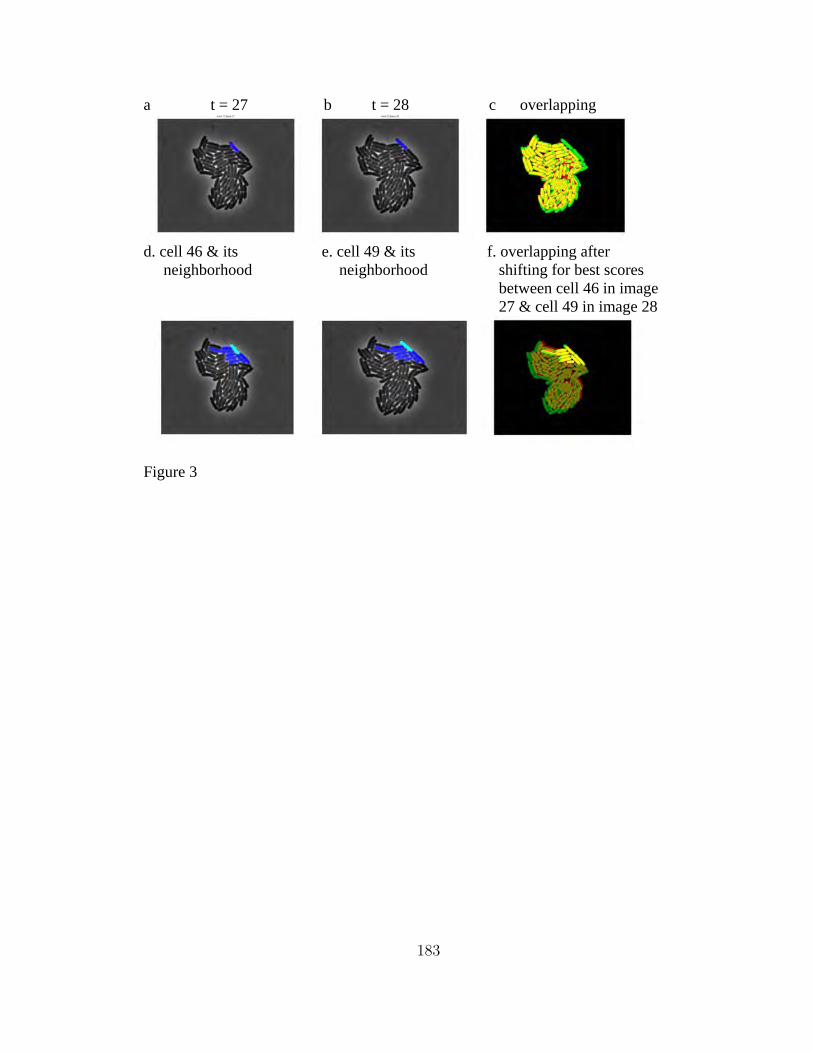
a t = 27 b t = 28 c overlapping
d. cell 46 & its e. cell 49 & its f. overlapping after neighborhood neighborhood shifting for best scores between cell 46 in image 27 & cell 49 in image 28
Figure 3
183

a. combined score matrix b. final correspondence matrix
c. lineage tree for cell 1 in the image 1.
Figure 4
184

a. Compared to Gordon method.
b. Compared to Sigal method.
Figure 5
185

Appendix F
A synthetic biology challenge: making cellscompute
The paper on the following pages was published in Tan et al. (2007).
186

A synthetic biology challenge: making cells compute Cheemeng Tan, Hao Song, Jarad Niemi, Lingchong You Abstract Advances in biology and engineering have enabled the reprogramming of cells with well-defined functions, leading to the emergence of synthetic biology. Early successes in this nascent field suggest its potential to impact diverse areas. Here, we examine the feasibility of engineering circuits for cell-based computation. We illustrate the basic concepts by describing the mapping of several computational problems to engineered gene circuits. Revolving around these examples and past studies, we discuss technologies and computational methods available to design, test, and optimize gene circuits. We conclude with discussion of challenges involved in a typical design cycle, as well as those specific to cellular computation. Keywords: synthetic biology, mathematical modeling, Bayesian statistics, information processing, cellular computing. Introduction
The last several years have witnessed the emergence of synthetic biology, a new area of biological research that aims to engineer gene circuits with desired functions for broad applications 1-6. This line of research has led to the development of diverse systems, such as oscillators7-9, communication-based circuits 10, 11, band detectors 11, bistable switches 12-15, ribo-switches 16-19, logic gates 20, 21, and drug-producing cells 22, 23. The broad spectrum of advances highlights the potential of the nascent field to impact diverse areas, including medicine 24, bioremediation 25, and computation 26.
Current computation is largely performed by digital computers with binary
information encoding. Information is transmitted and processed by electronic circuits, which can be arranged to eliminate crosstalk between signals and circuit components so as to minimize errors in information processing. It has been recognized that there are limitations to current digital computing technology: electronic circuits are often rigid and inflexible by design. They cannot evolve and adapt once implemented. Furthermore, computing is energy inefficient – even a desktop PC can consume significant amount of energy and generate waste heat. Furthermore, their architecture, which is largely based on sequential computation of complex tasks, may not be best suited for handling certain classes of computation 27-29. Finally, digital computers are believed to approach their computing speed limits due to constraints in miniaturization of transistors 30. These challenges have led to the development of new computing modes that build on alternative technologies, such as quantum computing 31 and DNA computing 32.
The advent of synthetic biology offers yet another opportunity to address
limitations of digital computation, which may ultimately lead to “cellular computation” 33.
187
At the outset, cells appear to possess some distinct advantages over digital computers. Cells can thrive in extreme environments, such as geysers with high temperatures 34, deep oceans with extreme pressures 35, and even nuclear plants filled with toxic chemicals 36. They can be readily engineered to sense and respond to diverse environmental signals. They can communicate with one another to exchange information about their environment 37, which enables coordinated population dynamics 38. In this scenario, a cell population can be considered as a vast collection of miniature computers working in parallel, where each consumes extremely minute amount of energy (at least in comparison to digital computers). Importantly, cells can adapt and evolve when they are challenged with new information that arises due to changes in nutrient abundance or temperature 39. This feature has been exploited to optimize cellular parts or gene circuits 40, 41
These apparent advantages suggest the appealing potential and opportunity of
using cells as programmable devices for computation. Neurobiology has a long history of considering neurons as computing units and extensive research is being carried out to decode mechanisms of such computing42-44. These studies have led to attempts to design simple chemical networks to implement basic computing tasks, such as a Turing machine45 and a frequency band-pass filter 46. Along another line of thinking, biological development has inspired the concept of “amorphous computing” that aims to generate coherent behavior from a group of unreliable and unknown parts, such as cells 47. Given the impressive advances in synthetic biology, it seems a natural next step to consider implementing computing tasks from bottom-up using well-defined synthetic gene circuits. Before engineering cells to perform human-defined computation, however, we must address several fundamental questions. For example, what kind of computational problems can we pose to cells in such a way to fully exploit their advantages? What are the fundamental challenges involved in cellular information processing and computation? Exploration of these issues will benefit from deeper understanding of how cells process information in nature, which may in turn offer inspiration for cellular computation. Cellular information processing
Cells process a plethora of environmental information relevant to their functions, such as variations in nutrients, growth factors, and temperature. This processing can be regarded as the flow of information from the extracellular environment, across the cell membrane and, through a series of signaling networks in the cytoplasm, finally initiating gene expression from the chromosome (Figure 1) 48. Extracellular information is received by cell membrane receptors and transformed into intracellular signals. For instance, binding of a specific ligand to a receptor can often trigger fast time-scale responses, such as methylation or phosphorylation of the intracellular domains of the receptor. These responses in turn can modulate downstream signaling cascades, leading to longer-term regulation of a diverse array of cellular components, such as kinases, phosphatases, secondary messengers, and transcription factors. Some proteins (e.g., kinases) can directly regulate cellular metabolic activities in the cytoplasm. Others (e.g., transcription factors) may translocate to the nucleus to activate gene expression. However, natural
188
information processing may bypass some steps in the generic architecture illustrated here. An extracellular molecule may diffuse across the cell membrane, activate a transcription regulator, and then initiate gene expression. This is a common mechanism of quorum sensing for many gram-negative bacteria. In this case, information processing bypasses many intermediate steps, for example the receptor-ligand binding reactions.
Natural cellular information processing exhibits several interesting features. In
particular, cells use various mechanisms to regulate information processing. This regulation may be conceptualized as being carried out by network motifs. A motif, such as feedback or feedforward regulation, is commonly defined as a small set of interactions among cellular components with a well-defined function 49-53. For example, positive feedback serves as the basis for ultrasensitive or bistable switches 54, 55. Negative feedback may reduce noise and introduce stability 56, but may also generate oscillations if a long time delay is involved 57. A wide variety of feedforward loops are also common in cellular networks and have diverse yet well-defined dynamic properties depending on their specific architecture58. Network motifs can be integrated to carry out more sophisticated cellular functions 50, 59. These may include cell cycle regulation, apoptosis, and differentiation.
Another feature of cellular information processing is parallelism, where a large
number of cells can carry out a certain function simultaneously. The parallelism is also evident when cells process complex information from diverse sources in parallel 60, 61. Such parallel information processing can be illustrated using the Escherichia coli chemotaxis pathway, by which E. coli cells sense extracellular stimuli and then migrate accordingly. Bacteria live in a dynamic environment with multiple conflicting stimuli, including chemoattractants and chemorepellents. These stimuli simultaneously bind to respective membrane receptors and initiate signaling cascades leading to phosphorylation or dephosphylation of a protein CheY. The extent of CheY phosphorylation modulates the frequency and direction of flagellar motor rotation, which then controls E. coli migration. Equipped with signaling cascades and gene regulatory networks, E. coli can respond flexibly to different streams of information in a complex and dynamic environment. Mapping computation to circuit engineering
The versatility of cells in information processing seems to suggest a great potential for cellular computation mediated by engineered gene circuits. One immediate set of questions then relates to the nature of computational problems for which cellular computation might be advantageous. Evidently, some initial examples would be various logic gates that have been proposed or implemented over the last few years 20, 26. Combinations of these logic gates can in principle serve as the basis for universal computation 62. To move towards more complex computation problems, however, we will need to develop much deeper understanding of how cells process information in natural contexts.
189

Here we attempt to map three commonly encountered computational problems (integration, optimization and signal-processing) to specific designs of gene circuits to illustrate the concept of cellular computation. For simplicity, we assume all these circuits are being implemented in E. coli, a major workhorse for synthetic biology research to date. These circuits (Figures 2-4) are hypothetical and their actual implementation may require fine-tuning or replacement of individual genetic components. However, we believe that these designs are within our reach given recent achievements in the field. Their implementation, if demonstrated to be functional, may open doors to exciting opportunities for cellular computation. Importantly, analysis and implementation of these circuits may offer insight into underlying mechanisms of nature cellular information processing. Integration
The aim is to compute the integral of a function )(xf in a limit, defined by h1(x), h2(x) and g(x) (Eq. 1 and Figure 2a).
∫ −=)(
)(
2
1
))()((Integralxh
xh
dxxgxf [1]
When )(xf and g(x) are simple functions, the integral is calculated easily with simple numerical methods such as the Simpson rule or the Trapezoidal rule. For more complex functions, such as ones encountered in quantum mechanics 63, the integral can often be approximated numerically using one of many Monte Carlo integration methods 64. The integral is essentially the area (Ω) as defined in Figure 2a. We now define an area Φ with well-defined dimensions that encloses Ω. Such algorithms evaluate multiple points in Φ and the points inside Ω will be registered as “hits”. In the simplest Monte Carlo method, the integral can then be calculated as the ratio of hits to the total number of points multiplied by Φ (Eq. 2). With this method, the approximation error decreases proportionally with increasing total number of points evaluated in Φ.
Φ=Φ=)coloniesall(#
)coloniesfluorecent(#points)(all#hits#Integral [2]
Such method can be readily mapped into cellular computation. For simplicity, we
consider a bounded area in an agar plate, covered by a uniform concentration of an immobilized ligand (Figure 2b). To “integrate”, we can engineer bacteria to carry a simple circuit that enables them to respond to the ligand by fluorescing (Figure 2c). By randomly plating these bacteria onto the agar surface, one can perform “integration” by simple colony counting: the integral can be estimated by the fraction of fluorescent colonies multiplied by the total area of the agar plate (Eq. 2). This simple system can be considered as an “integrator” and it can be implemented experimentally by using well-characterized inducible promoters. For illustration of the concept, colony counting on a surface will be convenient. However, the integration can also be carried out in three
190

dimensions to integrate over irregular volumes. In this case, one may first collect the bacteria and use flow cytometry to count the number of fluorescent bacteria.
We note that the non-trivial computational method can be mapped to an
apparently trivial biological circuit (an inducible promoter). This suggests that using cells to do what we normally consider as “computation” may be quite straightforward. By itself, a simple integrator will unlikely have any advantage over current computing methods. However, if cells can be engineered so that the integration result is connected to a physiological function, then cells can carry out real-time calculation and make decisions accordingly. For instance, one can imagine using a ligand to control a quorum sensing module to enable cell-cell communication. This configuration may allow cells to “calculate” the volume of an environment and act accordingly. In a sense, natural quorum sensing bacteria are constantly using such Monte Carlo type integration to probe their environments. Optimization
The notion of coupling environmental sensing and communication can lead to a gene circuit working as an “optimizer”. In an optimization problem as formulated in Eq. 3, the aim is to find the (x, y) value in a bounded search space that maximizes an objective function ),( yxF .
),(max: yxFObjecive [3]
For a simple ),( yxF with a distinct global maximum in the space, the problem
can be readily solved by using numerical methods such as interior point methods or simplex methods 65. These methods often fail for complex ),( yxF with multiple local maxima. In this case, the problem can be solved by using stochastic search algorithms such as simulated annealing 66, genetic algorithms 67, and swarm algorithms 68. These stochastic search algorithms are also Monte Carlo methods that depend on statistical sampling of a search space. Briefly, ),( yxF is evaluated at multiple points in the search space. The evaluations in each iteration are used to guide the search directions in the next iteration. The processes of evaluation and searching are repeated until the algorithm finds solutions that maximize ),( yxF . With limited computational resources, the success in locating the optimal solution will depend on the efficiency of “search” strategies. This efficiency can be improved by incorporating “communication” in the search process. That is, the algorithm integrates information from evaluations to choose appropriate search directions for the next iteration 68. In more mainstream statistical analysis, stochastic search methods are also coupled with Monte Carlo integration and "swarm-like" variants have proven most effective in even very challenging applications 69, 70.
Many such algorithms have been inspired from biological processes (e.g. swarm
algorithms and genetic algorithms) and they can be readily mapped back to cellular computation. ),( yxF can be represented by a distribution of ligand molecules on a
191
surface (Figure 3a). The molecules are immobilized and are not metabolized by cells. Bacteria can be engineered to respond to these molecules and adjust their motility (Figure 3b). This can be achieved by using the bacterial chemotaxis pathway that senses the ligand’s concentration gradient. In addition, they need to be engineered to communicate with one another, for example, by using a quorum sensing module. The communication will coordinate cells’ migration and increase the convergence rate of the population towards the optimal solution. In this design, we need to require that communication and ligand sensing be integrated at an AND gate. The AND gate can then be used to control chemotaxis by modulating the activity of key regulatory proteins, such as CheZ. This design aims to direct a cell population towards the optimal solution when both concentration gradient and cell density is high. We anticipate that cells regulated by this circuit will cluster significantly more than wild type cells at the globally optimal solution. As for any other complex gene circuit, successful implementation of the optimizer will require fine-tuning of circuit components to balance the amplitude and the signaling speed of both the ligand sensing module and the cell-cell communication module.
Some existing synthetic or natural circuits already possess partial characteristics
of an optimizer described above. For instance, Anderson et al. engineered bacteria to invade cancer cells by using either a hyposia-sensing module or a quorum sensing module 24. As such, the engineered bacteria will only invade cancer cells either under an anaerobic condition or when their density is high. Modification of the gene circuit by integrating hyposia-sensing and quorum-sensing at an AND gate may improve specificity of bacteria invasion of cancer cells. This modified circuit can be considered as an optimizer in which the bacteria locate the optimal solutions (the cancer cells) by detecting multiple input signals. Budrene and Berg have shown that bacteria aggregate at a local space by using both chemotaxis and self-secretion of a chemo-attractant71. In this case, bacteria become the source of attractant molecules to other cells, which further promotes bacteria chemotaxis towards a certain direction. Extension of this natural circuit by using a cell-cell communication module to control cell motility will also allow implementation of the optimizer. If we take lessons from performance of stochastic search algorithms, the integration of communication with motility behavior will likely improve ability of these cells to locate optimal solutions. However, this notion will require further investigation by modeling and experimentation. Fourier Transform
The first two examples will end up producing “steady-state” solutions of the computation problems. Natural information processing can also be carried out in the temporal domain. For example, consider an input signal represented by temporal fluctuations of a specific entity, such as electric pulses, concentrations of a molecule, or temperature. In many biological systems, an input signal can oscillate and its oscillation frequency may be critical. For example, during inflammatory response, expression of IL-2 and IL-8 cytokines peaks at an approximate [Ca2+] oscillation frequency of 0.01/second 72. In this case, one would wonder whether cells are processing frequency information, how they do it, and how we can achieve a similar task using synthetic circuits.
192

Computationally, frequency contents of an oscillatory signal x(t) can be analyzed
using the Fast Fourier Transform 73. The essence of this method is to compare similarity between the signal (x(t)) and a basis function (b(t)) (Eq. 4). Common basis functions include sine and cosine functions. A coefficient λ can be calculated to indicate similarity between x(t) and b(t). In this analysis, the signal-processing capacity is directly proportional to the number of basis functions: higher number of basis functions increases the temporal sensitivity of the signal analysis.
∫ •= dttbtx )()(λ [4]
To map this computational method into cellular computation, we can define a signal x(t) by changing the concentration of a signaling molecule (e.g., AHL) (Figure 4). We can then use a tunable natural or synthetic oscillator, such as the respressilator7 to generate oscillations in a transcription regulator LuxR (R) with different frequencies, which “implements” the basis functions b(t). In particular, we shall require AHL to activate LuxR (R*). If x(t) has the same frequency as b(t), we will expect the maximum concentration of active LuxR via a resonance effect. As a consequence, this can lead to maximum production of a fluorescent protein (GFP), whose concentration thus quantifies the similarity between x(t) and b(t). Based on the GFP concentration, we can identify b(t) with high similarity with x(t) and thus determine the frequency content of x(t). We shall refer to this circuit as a “signal processor”. We note that these concepts have been proposed in the context of chemical networks 46. Their experimental implementation with engineered gene circuits will pose new and exciting challenges to synthetic biologists.
Again, aspects of this computation process can be identified in numerous natural
biological processes, where cells process temporally changing information, for examples in circadian clocks 74, segmentation clocks 75, and Ca2+ signaling pathways 76. In these examples, several fundamental questions are yet to be elucidated. In particular, what is the speed limit of information processing in each system? What is the underlying mechanism of cells’ response to an oscillatory signal? That is, how do cells decode frequency signals? Active pursuit of these questions will not only enable us to better understand how natural signaling networks are evolved to accurately handle diverse information contents, but also benefit engineering of cell-based computation. Design cycle of synthetic gene circuits
Each of the three examples detailed above requires engineering of an appropriate gene circuit. Circuit engineering typically involves multiple rounds of a design cycle (see detailed review by Marguet et al.6). Given a conceptual design, mathematical modeling is often used to explore its dynamics, which may offer guidance for subsequent implementation, test, and revision. For circuits with complex dynamics, the role of modeling becomes even more critical. In addition to suggesting choices of appropriate circuit components to initiate implementation, modeling may also identify critical
193

components for further optimization, by rational design or directed evolution. Conversely, data collected from experimental tests of an initial implementation can provide valuable information for evaluating and revising mathematical models and circuit parameters. This may benefit from established statistical methods. Modeling-guided design
A wide spectrum of modeling methods, encompassing both deterministic and stochastic approaches, is available for circuit analysis. Interactions among circuit components can often be conveniently described by ordinary differential equations (ODE). An ODE model can be represented in a general form shown by Eq 5:
)~(~~CfV
dtCd
•= [5]
where C~ is a vector containing concentrations of each molecular species, t is time, V represents the stoichiometry matrix of reaction networks, and )~(~ Cf is a vector of expressions defining the rate of change for the concentration of each species.
When spatial transport of cellular components (e.g. by diffusion) plays a
significant role in a circuit function, partial differential equations (PDE) can be used. This method has been frequently used to analyze pattern formations in organism development 77, 78. Here, it would be most suited for analyzing the “optimizer”, where cells migration and quorum sensing signals diffusion are integral part of the circuit dynamics. Typically, this can be modeled by a diffusion-reaction model, as represented in a generic form in Eq 6.
)~(~~~2 CfVCD
dtCd
•+∇•= [6]
where D is a matrix containing diffusivity of each component, and C~2∇ is the Laplacian
ofC~ and it can be represented by 2
2
2
2 ~~
yC
xC
∂∂
+∂∂ in a two-dimensional Cartesian coordinate
system (x, y). Both ODE and PDE models are deterministic in the sense that, given the same
initial conditions for each model, repeated simulations will produce the same results. Both models can be analyzed by using two popular types of mathematical analysis: parametric sensitivity analysis and bifurcation analysis. Parametric sensitivity analysis can be carried out to characterize quantitative changes of circuit dynamics in response to perturbations of circuit parameters 79. This analysis is most helpful for identifying critical circuit components. Bifurcation analysis is used to determine how qualitative properties of a circuit depend on its parameters. Specifically, it aims to find the steady-state solutions of a system and their stability 80, 81. Bifurcation is said to occur when there is a change either in the number of steady state solutions or the stability of one or multiple solutions. For example, at a Hopf bifurcation point, a steady-state solution loses stability
194

and sustained oscillation arises. Bifurcation analysis can be used to analyze the oscillator module in the signal-processor mentioned above, by predicting effects of circuit parameters on the oscillation amplitude and frequency.
The differential equations (DE) framework may be inadequate when molecular
number of a species is low, which will generate “noise”, or stochastic fluctuations in cellular processes. When cellular noise drastically affects a circuit function, it has to be accounted for in the mathematical analysis. This can be carried out by chemical Langevin equations (CLE) or chemical master equations (CME) 82. In CLE, a noise term is appended explicitly to an ODE. A typical form of CLE is shown in Eq 7 82, 83.
)(~)~(~)~(~~tCfVCfV
dtCd ξ••+•= [7]
where the 2nd term captures intrinsic noise and )(~ tξ is the white noise with unit amplitude.
A CLE model can be solved numerically by algorithms derived for standard ODE models 84. In fact, it approximates a CME model, which captures the “true” stochastic dynamics of a system consisting of elementary reactions in homogenous environment. A CME model can be solved by using the Gillespie algorithm 85. Following a Monte Carlo scheme, this algorithm tracks firings of individual reactions and time intervals between these firings.
Similar to spatial extension of ODE to PDE, spatial effects can also be
incorporated into stochastic models. A spatial-stochastic model is particularly useful when noise affects reaction-diffusion dynamics of a molecule or a cell. This model has been applied to analyze intracellular signaling of MAPK cascades 86, segmentation dynamics of E. coli 87, and bacteria chemotaxis pathways 88. The model can be used to analyze the optimizer by predicting effects of noise on cells’ migration in a search space. Implementation
Many circuits may be constructed by combinations of existing genetic parts 5, 89. Currently, there are concerted efforts to collect, index, and standardize commonly used genetic parts as Biobricks, which include RBS sequences, promoter sequences, and protein coding sequences (http://parts.mit.edu/). Well-characterized Biobricks will drastically facilitate implementation of diverse gene circuits by not only serving as the elementary building materials, but also by providing critical kinetic parameters for initial modeling. At the next level, well-characterized devices and systems with a matching interface can be integrated to generate even more complex systems 1. For instance, implementation of the optimizer will require a quorum sensing module and an AND gate, as well as an interface to connect with the chemotaxis pathways.
Experimental test
195

Once a circuit is assembled, its performance can be evaluated by standard biological techniques, including assays for gene expression and cell growth. In particular, circuit engineering will benefit from recent development of an array of new detection technologies, including flow cytometry 90, light microscopy 91, and microfluidics 92. In a flow cytometer, each cell is passed through an excitation light source. The light scattering and emission data from the cells will be collected. This technology has been used widely to collect population statistics such as fluorescence distribution 12, 93 and cellular morphology 94, 95. Light microscopy is becoming an important tool for characterizing synthetic gene circuits. A distinct advantage of microscopy is that it can be used to track real-time cellular dynamics by recording time-lapse movies of engineered cells 7. This technique has been used to study noise in gene expression of a single cell 96, 97 and behavioral variations of bacteria chemotaxis activity 98.
In some cases, engineered cells have to be characterized under a variety of specific conditions for an extended period. Such tasks will benefit from recent development in microfluidics. Based on advances in microfabrication technologies, microfluidics is the design of miniaturized devices that handle samples at nanoliter volumes 92. One major impact of microfluidics on synthetic biology focuses on miniaturization of cell growth environment, in order to facilitate single cell measurements. For instance, Balagadde et al. used a microchemostat to characterize a population control circuit for hundreds of hours 99. Groisman et al. used a microfluidic device to maintain chemostatic conditions for bacteria and yeast growing in microchambers 100. Cookson et al. used a microchemostat to track gene expression of single yeast cells over multiple cell cycles101. Oloffson et al. created a chemical waveform synthesizer that can generate spatial chemical gradient on a microfluidic chip 102. These devices can be particularly useful for characterizing circuits involving sophisticated manipulation of experimental conditions, for instance, the signal processor. In this case, a chemical waveform synthesizer can be used to generate an oscillatory signal and the microchemostat can be used to maintain the signal processor, in order to process a signal for a long period of time. Model refinement guided by statistical methods
In the initial phase of mathematical modeling, reaction mechanisms and kinetic parameters are often derived from the literature or from the preliminary measurement of circuit components. Due to lack of quantitative information on cellular components (even standard parts), a model may not generate the “true” cellular dynamics as a result of parameter and model misspecification. In this case, and assuming adequacy of the overall functional form of the model, the analysis can be fine-tuned using statistical methods to fit the model to experimental measurements and refine understanding of relevant regions of parameter space. In the computational and technically attractive approach via Bayesian statistical methods, the steps involved are:
1) develop a statistical model representing errors of measurement, biological variability and parameter uncertainty,
196

2) summarize and represent existing biochemical information in terms of prior distributions, or more commonly classes of prior distributions, that reflect the substantive information and uncertainty about model parameters; 3) develop and understand the implied posterior distributions representing how the prior information is updated with experimental data to revise estimations and uncertainty measures about parameters -- typically this is carried out using Markov chain Monte Carlo (MCMC) techniques to simulate and summarize the statistical analysis 103, 104. 4) Explore aspects of model fit, both within models fit to training data and in using fitted models to predict test data, for evaluation and criticism of assumed model forms that may lead to model refinements. A statistical model, P(Y|θ), describes the relationship between the data Y to be
observed and a set of unknown parameters θ, in terms of a population sampling distribution of the data based on the mathematically specified model combined with statistical error components. For examples, suppose data are fluorescence levels for the integrator, spatial cell densities for the optimizer, or fluorescence levels through time for the signal-processor. One statistical model for the integrator is shown in Eq 8.
),()|( 2σβαθ cc xNYP += [8] where Yc is the background adjusted fluorescence level of cell c,
xc is 1 if cell c is bound to the ligand and 0 if not, N(μ,σ2) indicates a Gaussian distribution with mean μ and standard deviation σ, α is the mean fluorescence level of unbound cells, and α+β is the mean fluorescence level of ligand-bound cells.
If the cells are assumed to be independent, the full statistical model is as shown in
Eq 9. ∏=
ccYPYP )|()|( θθ
[9] After observing data, this is called the likelihood and is denoted L(θ), indicating
that it is a function of the parameters having been defined on the basis of this specific, now known and fixed data outcome.
Bayesian parameter estimation requires encoding initial scientific information
about parameters in a prior distribution that combines with the likelihood function to provide summary inferences. Repeat analysis with different models and priors is part of the natural, iterative model building process. Assuming one assigned prior denoted P(θ), analysis can proceed and then be repeated under variations of the prior and model. One typical approach is to choose priors under which component parameters are independent, viz P(θ) = P(α)P(β)P(σ). At this point, we can assign probability distributions that restrict the range of our parameters. For example, we may expect the fluorescence levels of proteins bound to the ligand to be higher than those that are not. Therefore a probability distribution should restrict the range of β to be positive. An example is to choose
197
P(β)=N(β0,σβ2)δ(β>0) where β0 is a prior point-estimate for β, σβ2 represents prior uncertainty about that estimate, and δ(β>0) is 1 whenever β>0 and 0 otherwise which restricts the range of β to the positive real numbers. Information from previous experimentation can be formally incorporated in this analysis through the prior. If we do not have any information about parameters, then we can use flat, non-informative priors.
After deriving the likelihood and assigning appropriate prior probability
distributions to our parameters, the statistical model is fully specified. The next step, although not trivial, involves only algebra and calculus to derive the posterior distribution, P(θ|X), of the parameters given the data. This is defined by Bayes' theorem as in Eq 10.
)()|()|( θθθ PXPXP ∝ [10] The posterior can only be derived and understood mathematically in the simplest
models. Nonetheless, MCMC and other numerical simulation methods can draw simulated values of the parameters from this posterior to obtain very large posterior samples. Such sampled parameter sets can be directly summarized – in terms of histograms, sample means, variances, quantiles and so forth -- to provide descriptions of what has been learned from the experimental data relative to the specific prior distributions chosen.
As mentioned, such formal statistical methods can suggest model refinements in
terms of suggesting different ranges of parameter values. For example, in the integrator, if the point-estimate for β is smaller then that for σ our signal-to-noise ratio will be very small. This indicates that the system requires cells that have a greater difference in fluorescence protein production between the ligand-bound and unbound states.
A variety of statistical models and data collection schemes can be developed to
answer different questions. For example, in the optimizer, we can collect cell density measurements at a single time point or we can collect time-course data, and develop rich classes of statistical models for biochemical parameter estimation and evaluation of specific mathematical model forms 105. Circuit optimization and revision Preliminary design and testing of an engineered circuit will allow us to pinpoint and modify specific circuit components, such as ribosomal binding sites, promoters, or genes. This can be carried out by structural based rational design, guided by molecular dynamic simulations. This strategy has been recently applied to engineer a bacterial membrane receptor to bind new ligands such as trinitrotoluene, l-lactate, and serotonin 106.
However, when detailed knowledge about a component’s structure is unavailable, directed evolution can be used to modify its function. Directed evolution optimizes a component according to a specific design objective. The optimization starts with generation of a component library by randomly changing its sequence, for example, by
198

using the error-prone PCR method107. The library is screened to identify component variants that can satisfy the design objective. For instance, Collins et al. used directed evolution to increase specificity of a LuxR protein to a specific target molecule, C8HSL, while maintaining its specificity to a wild type target, 3OC6HSL 40. The optimal LuxR proteins were selected based on their sensitivity to different dosage of C8HSL and 3OC6HSL. Similar approach has also been taken to optimize binding properties of receptor-ligand pairs 108, nucleic acid enzymes109, and a genetic circuit 41.
Challenges
While appealing, turning cells into computers will be tremendously challenging and requires deeper understanding of natural biological systems as well as new design strategies relevant to gene circuit engineering. In particular, what are the limits of cellular computation in terms of processing speed and accuracy? How do we control, modulate or exploit noise in cellular information processing? How can we increase robustness of a gene circuit, so that it will function properly under different conditions?
Computation speed is a critical factor in any computation. Cells running simple logic gates will not have advantages over digital computers – they would be too slow. Future cellular computation must be so designed to take advantage of the vast parallelism of cells. The parallelism can be exploited in algorithms that require a huge amount of simple calculations, such as the Monte Carlo type algorithms. This strategy is exemplified by the integrator and the optimizer. Still, the overall computation speed will benefit from optimization of individual components to increase their processing speed. This can be improved by increasing the production rate or the decay rate of a critical component in a circuit 110. It may also be modulated by incorporating network motifs such as negative feedback 111 or feed forward regulation58. Different cellular components will also have different intrinsic capabilities in terms of their processing speed. Signaling networks, which involve covalent modification of proteins (e.g. methylation and phosphyrlation), in general have much faster dynamics than gene expression.
Importantly, computation results will be affected by the presence of cellular noise.
As alluded earlier, cellular noise exists in the form of fluctuations in molecular concentration, which further leads to diverse cellular phenotypes 82, 112-117. Noise can be classified into two categories: the intrinsic noise, which arises from interactions between small numbers of interacting molecules; the extrinsic noise, which arises from fluctuations in the cellular environment 96. Noise can be both advantageous and disadvantageous in cellular computation. On one hand, noise is undesirable because it may reduce computation accuracy by causing randomness in gene expression. For instance, in the repressilator, noise affects the circuit’s function, resulting in only 40% of oscillating cells 7. In this case, noise is a serious concern in engineering of a reliable and tunable oscillator. On the other hand, noise might be beneficial to cellular computation by introducing behavioral variability. For instance, Blake et al. has shown that variability in gene expression increases the survival advantage of yeast cells under acute environment stress118. In the context of cellular computing, a heterogeneous optimizer population with
199

different migration rates and directions may allow cells to explore a bigger search space 98. This way, the optimizer will have a higher probability of finding the optimal solutions.
The impact of noise and other perturbations from the environment can be probed by sensitivity analysis, bifurcation analysis, or stochastic modeling, as described above. In most cases, we would want an engineered circuit to be robust, or insensitive, to such perturbations. To this end, noise can be modulated by different control strategies 82. For instance, it was demonstrated that negative feedback can reduce variability in gene expression 56. Cell-cell communication has been suggested as an effective strategy to couple cellular oscillators to realize synchronous oscillations119, 120. Other mechanisms, such as feedforward regulation 121 and gene dosage 122 may also enable further tuning of noise levels. Conclusion
Drawing inspiration from biology, computer science, mathematics, and engineering, we may one day engineer cells to solve computation problems that are difficult to solve using conventional methods. The engineering process may also help us to understand how cells perform computation in nature. In the long term, we envision the design of cellular computers, consisting of cells with specific computation roles such as integrator, optimizer, and signal-processor.
Acknowledgments We thank Mike West, John Pearson, and anonymous reviewers for critical reading of the manuscript and helpful discussions. This work was partially supported by the David and Lucile Packard Foundation, the National Institute of Health, and the National Science Foundation.
200

References 1. D. Endy, Nature, 2005, 438, 449-453. 2. S. A. Benner and A. M. Sismour, Nat Rev Genet, 2005, 6, 533-543. 3. G. M. Church, Mol Syst Biol, 2005, 1, 2005 0032. 4. R. McDaniel and R. Weiss, Curr Opin Biotechnol, 2005, 16, 476-483. 5. C. A. Voigt, Curr Opin Biotechnol, 2006, 17, 548-557. 6. P. Marguet, F. Balagadde, C. Tan and L. You, J R Soc Interface, 2007,
10.1098/rsif.2006.0206. 7. M. B. Elowitz and S. Leibler, Nature, 2000, 403, 335-338. 8. E. Fung, W. W. Wong, J. K. Suen, T. Bulter, S. G. Lee and J. C. Liao, Nature,
2005, 435, 118-122. 9. M. R. Atkinson, M. A. Savageau, J. T. Myers and A. J. Ninfa, Cell, 2003, 113,
597-607. 10. L. You, R. S. Cox, 3rd, R. Weiss and F. H. Arnold, Nature, 2004, 428, 868-871. 11. S. Basu, Y. Gerchman, C. H. Collins, F. H. Arnold and R. Weiss, Nature, 2005,
434, 1130-1134. 12. T. S. Gardner, C. R. Cantor and J. J. Collins, Nature, 2000, 403, 339-342. 13. A. Becskei, B. Seraphin and L. Serrano, Embo J, 2001, 20, 2528-2535. 14. B. P. Kramer and M. Fussenegger, Proc Natl Acad Sci U S A, 2005, 102, 9517-
9522. 15. F. J. Isaacs, J. Hasty, C. R. Cantor and J. J. Collins, Proc Natl Acad Sci U S A,
2003, 100, 7714-7719. 16. C. I. An, V. B. Trinh and Y. Yokobayashi, RNA, 2006, 12, 710-716. 17. F. J. Isaacs, D. J. Dwyer, C. Ding, D. D. Pervouchine, C. R. Cantor and J. J.
Collins, Nat Biotechnol, 2004, 22, 841-847. 18. T. S. Bayer and C. D. Smolke, Nat Biotechnol, 2005, 23, 337-343. 19. S. K. Desai and J. P. Gallivan, J Am Chem Soc, 2004, 126, 13247-13254. 20. C. C. Guet, M. B. Elowitz, W. Hsing and S. Leibler, Science, 2002, 296, 1466-
1470. 21. R. Weiss, Ph.D.Thesis, Massachusetts Institute of Technology, 2001. 22. D. K. Ro, E. M. Paradise, M. Ouellet, K. J. Fisher, K. L. Newman, J. M. Ndungu,
K. A. Ho, R. A. Eachus, T. S. Ham, J. Kirby, M. C. Chang, S. T. Withers, Y. Shiba, R. Sarpong and J. D. Keasling, Nature, 2006, 440, 940-943.
23. E. S. Gilbert, A. W. Walker and J. D. Keasling, Appl Microbiol Biotechnol, 2003, 61, 77-81.
24. J. C. Anderson, E. J. Clarke, A. P. Arkin and C. A. Voigt, J Mol Biol, 2006, 355, 619-627.
25. M. Urgun-Demirtas, B. Stark and K. Pagilla, Crit Rev Biotechnol, 2006, 26, 145-164.
26. R. Weiss, S. Basu, S. Hooshangi, A. Kalmbach, D. Karig, R. Mehreja and I. Netravali, Natural Computing, 2003, 47-84.
27. J. Backus, Communications of the ACM, 1978, 21, 613-641. 28. M. Sipper, Computer, 1999, 32, 18-26.
201

29. P. Wegner and D. Goldin, Communications of the ACM, 2003, 46, 100-102. 30. N. Forbes and M. Foster, Computing in Science & Engineering, 2003, 5, 18- 19. 31. M. Hirvensalo, Quantum Computing 1st edn., Springer-Verlag, 2001. 32. A. J. Ruben and L. F. Landweber, Nat Rev Mol Cell Biol, 2000, 1, 69-72. 33. M. L. Simpson, G. S. Sayler, J. T. Fleming and B. Applegate, Trends Biotechnol,
2001, 19, 317-323. 34. R. Lieph, F. A. Veloso and D. S. Holmes, Trends Microbiol, 2006, 14, 423-426. 35. K. Horikoshi, Curr Opin Microbiol, 1998, 1, 291-295. 36. D. Appukuttan, A. S. Rao and S. K. Apte, Appl Environ Microbiol, 2006. 37. B. L. Bassler, Cell, 2002, 109, 421-424. 38. A. M. Lazdunski, I. Ventre and J. N. Sturgis, Nat Rev Microbiol, 2004, 2, 581-592. 39. H. H. McAdams, B. Srinivasan and A. P. Arkin, Nat Rev Genet, 2004, 5, 169-178. 40. C. H. Collins, F. H. Arnold and J. R. Leadbetter, Mol Microbiol, 2005, 55, 712-
723. 41. Y. Yokobayashi, R. Weiss and F. H. Arnold, Proc Natl Acad Sci U S A, 2002, 99,
16587-16591. 42. J. V. Neumann, The Computer and the Brain, 2nd edn., Yale University Press,
1958. 43. L. F. Abbott and W. G. Regehr, Nature, 2004, 431, 796-803. 44. M. London and M. Hausser, Annu Rev Neurosci, 2005, 28, 503-532. 45. A. Hjelmfelt, E. D. Weinberger and J. Ross, Proc Natl Acad Sci U S A, 1992, 89,
383-387. 46. M. Samoilov, A. Arkin and J. Ross, J. Phys. Chem. A, 2002, 106, 10205-10221. 47. H. Abelson, D. Allen, D. Coore, C. Hanson, G. Homsy, T. F. Knight, R. Nagpal,
E. Rauch, G. J. Sussman and R. Weiss, Communications of the ACM, 2001, 43. 48. J. Downward, Nature, 2001, 411, 759-762. 49. C. V. Rao and A. P. Arkin, Annu Rev Biomed Eng, 2001, 3, 391-419. 50. D. M. Wolf and A. P. Arkin, Curr Opin Microbiol, 2003, 6, 125-134. 51. H. M. Sauro and B. N. Kholodenko, Prog Biophys Mol Biol, 2004, 86, 5-43. 52. A. Ma'ayan, R. D. Blitzer and R. Iyengar, Annu Rev Biophys Biomol Struct, 2005,
34, 319-349. 53. J. J. Tyson, K. C. Chen and B. Novak, Curr Opin Cell Biol, 2003, 15, 221-231. 54. J. E. Ferrell, Jr., Curr Opin Cell Biol, 2002, 14, 140-148. 55. U. S. Bhalla and R. Iyengar, Science, 1999, 283, 381-387. 56. A. Becskei and L. Serrano, Nature, 2000, 405, 590-593. 57. A. Goldbeter, Biochemical oscillations and cellular rhythms, Cambridge
University Press, 1996. 58. S. Mangan and U. Alon, Proc Natl Acad Sci U S A, 2003, 100, 11980-11985. 59. L. H. Hartwell, J. J. Hopfield, S. Leibler and A. W. Murray, Nature, 1999, 402,
C47-52. 60. R. B. Bourret and A. M. Stock, J Biol Chem, 2002, 277, 9625-9628. 61. J. D. Jordan, E. M. Landau and R. Iyengar, Cell, 2000, 103, 193-200. 62. N. E. Buchler, U. Gerland and T. Hwa, Proc Natl Acad Sci U S A, 2003, 100,
5136-5141.
202

63. N. A. Benedek, I. K. Snook, M. D. Towler and R. J. Needs, J Chem Phys, 2006, 125, 104302.
64. C. P. Robert and G. Casella, Monte Carlo Statistical Methods, 2 edn., Springer, 2005.
65. D. Bertsimas and J. N. Tsitsiklis, Introduction to Linear Optimization, Athena Scientific, 1997.
66. S. Kirkpatrick, C. Gelatt and M. Vecchi, Science, 1983. 67. D. E. Goldberg, Genetic Algorithms in Search, Optimization and Machine
Learning, Kluwer Academic Publishers, Boston, 1989. 68. J. Kennedy and R. Eberhart, Proc IEEE Intl Conference Neural Networks, 1995,
1942-1948. 69. B. Jones, A. Dobra, C. Carvalho, C. Hans, C. Carter and M. West, Statistical
Science, 2005, 20, 388-400. 70. C. Hans, A. Dobra and M. West, Journal of the American Statistical Association,
in press, 2007. 71. E. O. Budrene and H. C. Berg, Nature, 1991, 349, 630-633. 72. R. E. Dolmetsch, K. Xu and R. S. Lewis, Nature, 1998, 392, 933-936. 73. A. V. Oppenheim, R. W. Schafer and J. R. Buck, Discrete-Time Signal
Processing, 2nd edn., Prentice Hall, 1999. 74. S. L. Harmer, S. Panda and S. A. Kay, Annu Rev Cell Dev Biol, 2001, 17, 215-253. 75. O. Pourquie, Science, 2003, 301, 328-330. 76. M. J. Berridge, M. D. Bootman and H. L. Roderick, Nat Rev Mol Cell Biol, 2003,
4, 517-529. 77. H. Meinhardt, Models of biological pattern formation, Academic Press, London ;
New York, 1982. 78. G. T. Reeves, C. B. Muratov, T. Schupbach and S. Y. Shvartsman, Dev Cell, 2006,
11, 289-300. 79. A. Varma, M. Morbidelli and H. Wu, Parametric sensitivity in chemical systems,
Cambridge University Press, Cambridge, U.K. ; New York, 1999. 80. J. Guckenheimer and P. Holmes, Nonlinear oscillations, dynamical systems, and
bifurcations of vector fields, Corr. 7th print. edn., Springer, New York, 2002. 81. Y. A. Kuznetsov, Elements of applied bifurcation theory, 3rd edn., Springer-
Verlag, New York, 2004. 82. C. V. Rao, D. M. Wolf and A. P. Arkin, Nature, 2002, 420, 231-237. 83. D. T. Gillespie, J. Chem. Phys., 2000, 113, 297-306. 84. P. E. Kloeden, E. Platen and H. Schurz, Numerical solution of SDE through
computer experiments, Springer-Verlag, Berlin ; New York, 1994. 85. D. T. Gillespie, The journal of physical chemistry, 1977, 81, 2340-2361. 86. K.-H. Chiam, C. M. Tan, V. Bhargava and G. Rajagopal, Physical Review E,
2006, 74. 87. D. Fange and J. Elf, PLoS Comput Biol, 2006, 2, e80. 88. T. S. Shimizu, S. V. Aksenov and D. Bray, J Mol Biol, 2003, 329, 291-309. 89. N. J. Guido, X. Wang, D. Adalsteinsson, D. McMillen, J. Hasty, C. R. Cantor, T.
C. Elston and J. J. Collins, Nature, 2006, 439, 856-860.
203

90. H. M. Davey and D. B. Kell, Microbiol Rev, 1996, 60, 641-696. 91. D. J. Stephens and V. J. Allan, Science, 2003, 300, 82-86. 92. D. N. Breslauer, P. J. Lee and L. P. Lee, Mol Biosyst, 2006, 2, 97-112. 93. H. Kobayashi, M. Kaern, M. Araki, K. Chung, T. S. Gardner, C. R. Cantor and J.
J. Collins, Proc Natl Acad Sci U S A, 2004, 101, 8414-8419. 94. P. O. Krutzik and G. P. Nolan, Cytometry A, 2003, 55, 61-70. 95. D. A. Veal, D. Deere, B. Ferrari, J. Piper and P. V. Attfield, J Immunol Methods,
2000, 243, 191-210. 96. M. B. Elowitz, A. J. Levine, E. D. Siggia and P. S. Swain, Science, 2002, 297,
1183-1186. 97. N. Rosenfeld, J. W. Young, U. Alon, P. S. Swain and M. B. Elowitz, Science,
2005, 307, 1962-1965. 98. E. Korobkova, T. Emonet, J. M. Vilar, T. S. Shimizu and P. Cluzel, Nature, 2004,
428, 574-578. 99. F. K. Balagadde, L. You, C. L. Hansen, F. H. Arnold and S. R. Quake, Science,
2005, 309, 137-140. 100. A. Groisman, C. Lobo, H. Cho, J. K. Campbell, Y. S. Dufour, A. M. Stevens and
A. Levchenko, Nat Methods, 2005, 2, 685-689. 101. S. Cookson, N. Ostroff, W. L. Pang, D. Volfson and J. Hasty, Mol Syst Biol, 2005,
1, 2005 0024. 102. J. Olofsson, H. Bridle, J. Sinclair, D. Granfeldt, E. Sahlin and O. Orwar, Proc
Natl Acad Sci U S A, 2005, 102, 8097-8102. 103. A. Gelman, J. B. Carlin, H. S. Stern and D. B. Rubin, Bayesian Data Analysis,
2nd edn., Chapman & Hall, New York, 2004. 104. Y. J. Jiang, B. L. Aerne, L. Smithers, C. Haddon, D. Ish-Horowicz and J. Lewis,
Nature, 2000, 408, 475-479. 105. D. J. Wilkinson, Stochastic Modelling for Systems Biology, 1st edn., Chapman &
Hall/CRC, Boca Raton, 2006. 106. L. L. Looger, M. A. Dwyer, J. J. Smith and H. W. Hellinga, Nature, 2003, 423,
185-190. 107. R. C. Cadwell and G. F. Joyce, PCR Methods Appl, 1994, 3, S136-140. 108. K. Chockalingam, Z. Chen, J. A. Katzenellenbogen and H. Zhao, Proc Natl Acad
Sci U S A, 2005, 102, 5691-5696. 109. G. F. Joyce, Annu Rev Biochem, 2004, 73, 791-836. 110. R. T. Schimke, Curr. Top. Cell. Regul., 1969, 1, 77–124. 111. N. Rosenfeld, M. B. Elowitz and U. Alon, J Mol Biol, 2002, 323, 785-793. 112. H. H. McAdams and A. Arkin, Proc Natl Acad Sci U S A, 1997, 94, 814-819. 113. I. R. Booth, Int J Food Microbiol, 2002, 78, 19-30. 114. A. Aertsen and C. W. Michiels, Crit Rev Microbiol, 2004, 30, 263-273. 115. H. Maughan and W. L. Nicholson, J Bacteriol, 2004, 186, 2212-2214. 116. E. M. Ozbudak, M. Thattai, I. Kurtser, A. D. Grossman and A. van Oudenaarden,
Nat Genet, 2002, 31, 69-73. 117. W. J. Blake, K. A. M, C. R. Cantor and J. J. Collins, Nature, 2003, 422, 633-637.
204

118. W. J. Blake, G. Balazsi, M. A. Kohanski, F. J. Isaacs, K. F. Murphy, Y. Kuang, C. R. Cantor, D. R. Walt and J. J. Collins, Mol Cell, 2006, 24, 853-865.
119. D. McMillen, N. Kopell, J. Hasty and J. J. Collins, Proc Natl Acad Sci U S A, 2002, 99, 679-684.
120. J. Garcia-Ojalvo, M. B. Elowitz and S. H. Strogatz, Proc Natl Acad Sci U S A, 2004, 101, 10955-10960.
121. B. Ghosh, R. Karmakar and I. Bose, Phys Biol, 2005, 2, 36-45. 122. D. L. Cook, A. N. Gerber and S. J. Tapscott, Proc Natl Acad Sci U S A, 1998, 95,
15641-15646.
205

Figure legend Figure 1: Information flow in a cell. Upon binding with extracellular signals, cell
membrane receptors activate downstream signaling molecules. These signaling molecules (e.g., kinase, phosphotase, etc.) are further processed by signaling cascades in the cytoplasm. These components may subsequently activate transcription factors, which in turn activate gene expression.
Figure 2: An integrator. (a) The integration is defined as the limit sum of f(x) minus
g(x), bounded by h1(x) and h2(x). (b) An area Ω (a subset of an area Φ) will be covered by uniform concentration of a specific ligand. (c) Cells can be engineered with a simple circuit that enables them to respond to the ligand by fluorescing. To “integrate”, these cells can be randomly plated onto the surface. The integral can be calculated as fraction of the fluorescent colonies multiplied by Φ.
Figure 3: An optimizer. (a) We aim to find an optimal solution (x,y) that maximizes a
function F(x,y). The function F(x,y) can be represented by distribution of a specific ligand on a surface. (b) Cells can be engineered to sense the ligand concentration gradient and communicate with each other, and adjust their motility accordingly. Signals from ligand sensing and communication can be integrated at an AND gate, which modulates the activity of key chemosensory components, such as CheZ. The modulation aims to direct a cell migration towards a space with higher ligand concentration gradient and higher cell density. As a consequence of ligand sensing and communication, cells are expected to cluster around the position with the highest ligand concentration, thus realizing the optimization task.
Figure 4: A signal processor. We can define an input signal x(t) by concentration
changes of an AHL molecule. A natural or synthetic oscillator can be used to generate oscillations in LuxR with different frequencies. Each oscillation with a specific frequency serve as a basis function (b(t)). If AHL has the same frequency as LuxR, we will expect maximum amount of activated LuxR (R*) molecules. This will lead to maximum expression of a green fluorescent protein (GFP). The fluorescent intensity can then represent the similarity between the x(t) and a particular b(t). Since we know the frequency content of b(t), we will be able to extract the frequency power spectrum of the x(t). For clarity, we have shown one basis function. With a tunable oscillator, multiple basis functions with different frequencies can be generated.
206

Figure 1
Cell membrane
Receptor ligand interaction
Extracellular signals
Signaling cascades
Gene expression
Nucleus
Cytoplasm
207

`
`
Figure 2
(b)
ΩColonies
Ligand
(a)
Φ
x
y
f(x)
g(x)
h1(x) h2(x)
Ω
Φ
GFP
gfp
Receptor
Ligand(c)
208

),(max:yxF
Objecive
Ligand
Figure 3
Ligand concentration
Optimal Solution(a)
(b)
FlagellaAHL
Quorum Sensing
Ligand SensingAND GateChemotaxis
209
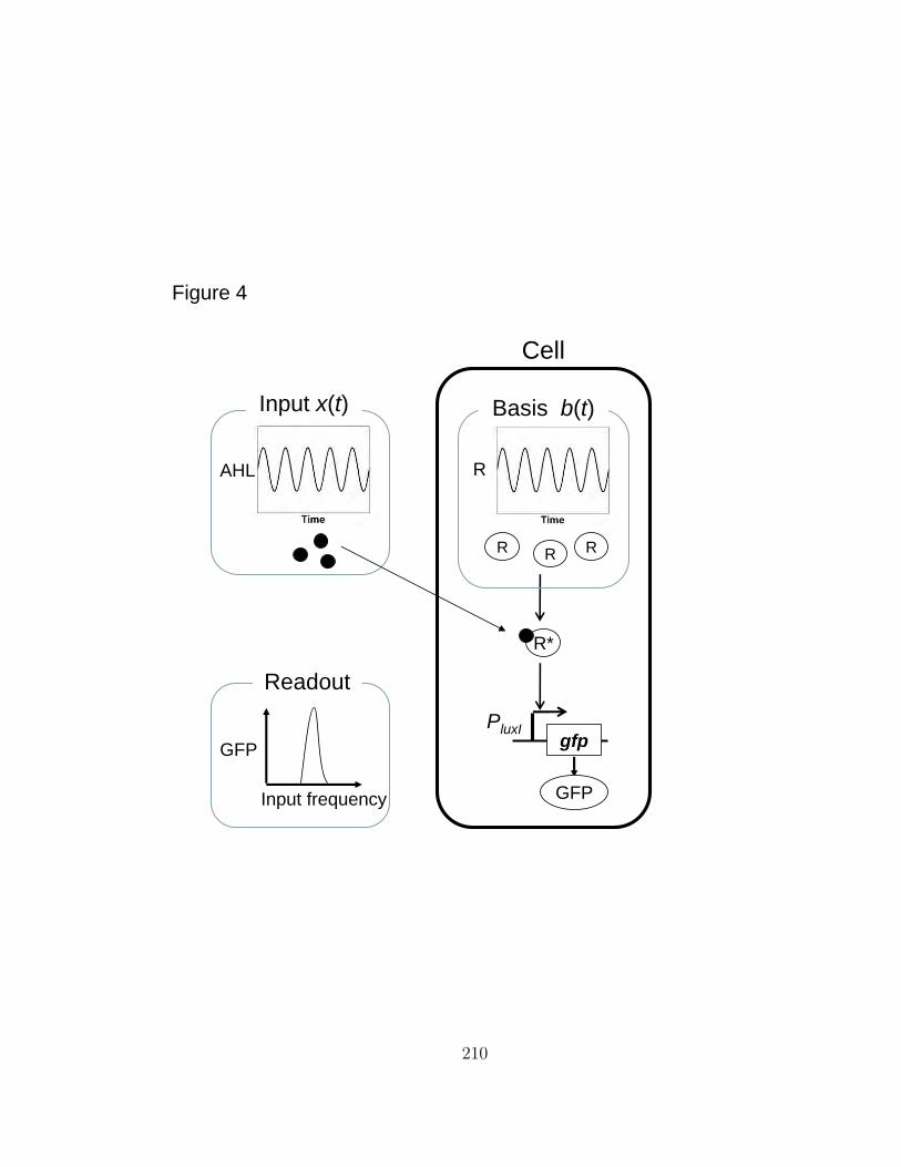
PluxI
Input frequency
Figure 4
R
AHL R
R R
R*
gfp
GFP
Input x(t) Basis b(t)
Cell
GFP
Readout
210

Bibliography
Alspach, D. L. and Sorenson, H. W. (1972), “Nonlinear Bayesian estimation usingGaussian sum approximations,” IEEE Transactions on Automatic Control, AC-17,439–448.
Arasaratnam, I., Haykin, S., and Elliott, R. (May 2007), “Discrete-time nonlinearfiltering algorithms using Gauss-Hermite quadrature,” Proceedings of the IEEE,95, 953–977.
Baccam, P., Beauchemin, C., Macken, C. A., Hayden, F. G., and Perelson, A. S.(2006), “Kinetics of influenza A virus infections in humans,” Journal of Virology,80, 7590–7599.
Beskos, A., Papaspiliopoulos, O., Roberts, G. O., and Fearnhead, P. (2006), “Exactand computationally efficient likelihood-based estimation for discretely observeddiffusion processes (with discussion),” Journal of the Royal Statistical Society:Series B (Statistical Methodology), 68, 333–382.
Bild, A. H., Yao, G., Chang, J. T., Wang, Q., Potti, A., Chasse, D., Joshi, M.,Harpole, D., Lancaster, J. M., Berchuck, A., Olson, J. A., Marks, J. R., Dressman,H. K., West, M., and Nevins, J. (2006), “Oncogenic pathway signatures in humancancers as a guide to targeted therapies,” Nature, 439, 353–357.
Boys, R. J., Wilkinson, D. J., and Kirkwood, T. B. (2008), “Bayesian inferencefor a discretely observed stochastic kinetic model,” Statistics and Computing, 18,125–135.
Brady, S., Orlando, D., J.Y., L., Wang, J., Koch, J., Dinneny, J., Mace, D., Ohler,U., and Benfey, P. (2007), “A high-resolution root spatiotemporal map revealsdominant expression patterns,” Science, 318, 801–806.
Burkom, H. (2007), “Alerting algorithms for biosurveillance,” in Disease surveillance,eds. J. S. Lombardo and D. Buckeridge, pp. 143–192, Wiley, New York.
Carlin, B. P., Polson, N. G., and Stoffer, D. S. (1992), “A Monte Carlo approach tononnormal and nonlinear state-space modeling,” Journal of the American Statis-tical Association, 87, 493–500.
211

Carpenter, J., Clifford, P., and Fearnhead, P. (1999), “An improved particle filter fornon-linear problems,” IEE Proc., Radar Sonar Navigation, 146, 2 – 7.
Carter, C. K. and Kohn, R. (1994), “On Gibbs sampling for state space mdoels,”Biometrika, 81, 541–553.
Carvalho, C. M. and Lopes, H. F. (2007), “Doi:10.1016/J.Csda.2006.07.019,” 51,4526 – 4542.
Carvalho, C. M., Johannes, M., Lopes, H. F., and Polson, N. (2008), “Particle learn-ing and smoothing,” Duke statistics discussion paper 2008-32.
Chen, R. and Liu, J. S. (2000), “Mixture Kalman filters,” Journal of the RoyalStatistical Society: Series B (Statistical Methodology), 62, 493–508.
Chesney, M. and Scott, L. O. (1989), “Pricing European options: A comparisonof the modified Black-Scholes model and a random variance model,” J. Financ.Qualitat Anal, 24, 267–284.
Chib, S., Nardari, F., and Shephard, N. (2002), “Markov chain Monte Carlo methodsfor stochastic volatility models,” Journal of Econometrics, 108, 281–316.
Choi, K. and Thacker, S. b. (1981), “An evaluation of influenza mortality surveil-lance, 1962-1979: ii. percentage of pneumonia and influenza deaths as an indicatorof influenza activity,” Am. J. Epidemiol., 113, 227–235.
Connors, K. A. (1990), Chemical Kinetics: The Study of Reaction Rates in Solution,John Wiley and Sons, Inc., New York.
Cooper, B. and Lipsitch, M. (2004), “The analysis of hospital infection data usinghidden Markov models,” Biostat, 5, 223–237.
Cowling, B. J., Wong, I. O. L., Ho, L.-M., Riley, S., and Leung, G. M. (2006),“Methods for monitoring influenza surveillance data,” International Journal ofEpidemiology, 35, 1314–1321.
Danielsson, J. (1994), “Stochastic volatility in asset prices: estimation with simulatedmaximum likelihood,” Journal of Econometrics, 61, 375–400.
Danielsson, J. and Richard, J.-F. (1993), “Quadratic acceleration for simulated max-imum likelihood evaluation,” Journal of Applied Econometrics, 8, 153–173.
De Jong, P. and Shephard, N. (1995), “The simulation smoother for time seriesmodels,” Biometrika, 82, 339–350.
Doucet, A., Godsill, S., and Andrieu, C. (2000), “On sequential Monte Carlo sam-pling methods for Bayesian filtering,” Statistics and Computing, 10, 197–208.
212
Doucet, A., De Freitas, N., and Gordon, N. (2001), Sequential Monte Carlo Methodsin Practice, Springer-Verlag, New York.
Farinha, J. P. S., Martinho, J. M. G., and Pogliani, L. (1997), “Non-linear least-squares and chemical kinetics. An improved method to analyse monomer-excimerdecay data,” Journal of Mathematical Chemistry, 21, 131–139.
Farrington, C. P., Andrews, N. J., Beale, A. D., and Catchpole, M. A. (1996), “Astatistical algorithm for the early detection of outbreaks of infectious disease,”Journal of the Royal Statistical Society, A, 159, 547–563.
Fearnhead, P. (2002), “Markov chain Monte Carlo, sufficient statistics, and particlefilters,” Journal of Computational and Graphical Statistics, 11, 848–862.
Ferreira, M. A. R. and Lee, H. K. H. (2007), Multiscale Modeling: A BayesianPerspective, Springer, New York.
Ferreira, M. A. R., West, M., Lee, H. K. H., and Higdon, D. M. (2006), “Multi-scaleand hidden resolution time series models,” Bayesian Analysis, 1, 947–968.
Frisn, M. (2003), “Statistical surveillance. Optimality and methods,” InternationalStatistical Review, 71, 403–434.
Fruhwirth-Schnatter, S. (1994), “Data augmentation and dynamic linear models,”Journal of Time Series Analysis, 15, 183–202.
Gelfand, A. E. and Smith, A. F. M. (1990), “Sampling-based approaches to cal-culating marginal densities,” Journal of the American Statistical Association, 85,398–409.
Gelman, A., Roberts, G. O., and Gilks, W. R. (1996), “Efficient Metropolis JumpingRules,” in Bayesian Statistics 5 – Proceedings of the Fifth Valencia InternationalMeeting, eds. J. M. Bernardo, J. O. Berger, A. P. Dawid, and A. F. M. Smith, pp.599–607, Clarendon Press [Oxford University Press].
Geman, S. and Geman, D. (1984), “Stochastic relaxation, Gibbs distributions, andthe Bayesian restoration of images,” IEEE Transactions on Pattern Analysis andMachine Intelligence, 6, 721–741.
Geweke, J. (1989), “Bayesian inference in econometric models using Monte Carlointegration,” Econometrica, 57, 1317–1339.
Gillespie, D. T. (1977), “Exact stochastic simulation of coupled chemical reactions,”Journal of Physical Chemistry, 81, 2340–2361.
Gillespie, D. T. (2007), “Stochastic simulation of chemical kinetics,” Annual Reviewsin Physical Chemistry, 58, 35–55.
213
Ginsberg, J., Mohebbi, M. H., Patel, R. S., Brammer, L., Smolinski, M. S., and Bril-liant, L. (2009), “Detecting influenza epidemics using search engine query data,”Nature, 457, 1012–1014.
Godsill, S. J., Doucet, A., and West, M. (2004), “Monte Carlo smoothing for non-linear time series,” Journal of the American Statistical Association, 99, 156–168.
Golightly, A. and Wilkinson, D. J. (2005), “Bayesian inference for stochastic kineticmodels using a diffusion approximation,” Biometrics, 61, 781–788.
Golightly, A. and Wilkinson, D. J. (2006a), “Bayesian sequential inference for non-linear multivariate diffusions,” Statistics and Computing, 16, 323–338.
Golightly, A. and Wilkinson, D. J. (2006b), “Bayesian sequential inference forstochastic kinetic biochemical network models,” Journal of Computational Biology,13, 838–851.
Golightly, A. and Wilkinson, D. J. (2008), “Bayesian inference for nonlinear mul-tivariate diffusion models observed with error,” Comput. Stat. Data Anal., 52,1674–1693.
Gordon, N. J., Salmond, D. J., and Smith, A. F. M. (1993), “Novel approachto nonlinear/non-Gaussian Bayesian state estimation,” IEE Proceedings Part F:Communications, Radar and Signal Processing, 140, 107–113.
Haario, H., Saksman, E., and Tamminen, J. (2001), “An Adaptive Metropolis Algo-rithm,” Bernoulli, 7, 223–242.
Haley, K. J., Stuart, J. R., Raymond, J. D., Niemi, J. B., and Simmons, M. J.(2005), “Impairment of cytotype regulation of P -element activity in Drosophilamelanogaster by mutations in the Su(var)205 gene.” Genetics, 171, 583–595.
Harrison, P. and Stevens, C. (1971), “A Bayesian approach to short-term forecast-ing,” Operations Research Quarterly, 22, 341–362.
Harrison, P. and Stevens, C. (1976), “Bayesian forecasting,” Journal of the RoyalStatistical Society B, 38, 205–247, (with discussion).
Harvey, A., Koopman, S. J., and Shephard, N. (2004), State Space and UnobservedComponent Models, Cambridge University Press.
Harvey, A. C., Ruiz, E., and Shephard, N. (1994), “Multivariate stochastic variancemodels,” Review of Economic Studies, 61, 247–264.
Hastings, W. K. (1970), “Monte Carlo sampling methods using Markov chains andtheir applications,” Biometrika, 57, 97–109.
214

Held, L., Hohle, M., and Hofmann, M. (2005), “A statistical framework for the anal-ysis of multivariate infectious disease surveillance counts,” Statistical modelling, 5,187–199.
Helfenstein, U. (1986), “Box-Jenkins modelling of some viral infectious diseases,”Statistics in Medicine, 5, 37–47.
Higuchi, T. (1997), “Monte Carlo filter using the genetic algorithm operators,” J.Statist. Comput. Simul., 59, 1–23.
Hohle, M. (2007), “surveillance: An R package for the monitoring of infectiousdiseases,” Computational Statistics, 22, 571–582.
Hull, J. and White, A. (1987), “Hedging the risk for writing foreign currency options,”J. Int. Money Finance, 6, 131–152.
Hurzeler, M. and Kunsch, H. R. (1998), “Monte Carlo approximations for generalstate-space models,” Journal of Computational and Graphical Statistics, 7, 175–193.
Ito, K. and Xiong, K. (2000), “Gaussian filters for nonlinear filtering problems,”IEEE Tans. Autom. Control, 45, 910–927.
IUPAC (1997), Compendium of Chemical Terminology, Blackwell Scientific Publica-tions, Oxford, 2nd edn., Compiled by A. D. McNaught and A. Wilkinson. XMLon-line corrected version: http://goldbook.iupac.org (2006-) created by M. Nic, J.Jirat, B. Kosata; updates compiled by A. Jenkins.
Jacquier, E., Polson, N. G., and Rossi, P. E. (1994), “Bayesian analysis of stochasticvolatility models,” Journal of Business and Economic Statistics, 12, 372–289.
Jacquier, E., Polson, N. G., and Rossi, P. E. (2004), “Bayesian analysis of stochasticvolatility models with fat-tails and correlated errors,” Journal of Econometrics,122, 185–212.
Julier, S. and Uhlmann, J. (1997), “A new extension of the Kalman filter to nonlinearsystems,” in Int. Symp. Aerospace/Defense Sensing, Simul. and Controls, Orlando,FL.
Jungbacker, B. and Koopman, S. J. (2007), “Monte Carlo estimation for nonlinearnon-Gaussian state space models,” Biometrika, 94, 827–839.
Kalman, R. E. (1960), “A New Approach to Linear Filtering and Prediction Prob-lems,” Transactions of the ASME–Journal of Basic Engineering, 82, 35–45.
Kim, S., Shephard, N., and Chib, S. (1998), “Stochastic volatility: likelihood in-ference and comparison with ARCH models,” Review of Economic Studies, 65,
215

361–393.
Kitagawa, G. (1996), “Monte Carlo filter and smoother for non-Gaussian nonlinearstate space models,” Journal of Computational and Graphical Statistics, 5, 1–25.
Knorr-Held, L. and Richardson, S. (2003), “A hierarchical model for space-timesurveillance data on meningococcal disease indicence,” Applied statistics, 52, 169–83.
Kong, A., Liu, J. S., and Wong, W. H. (1994), “Sequential imputations and Bayesianmissing data problems,” Journal of the American Statistical Association, 89, 278–288.
Le Strat, Y. and Carrat, F. (1999), “Monitoring epidemiologic surveillance data usinghidding Markov models,” Statistics in medicine, 18, 3463–3478.
LeStart, Y. (2005), “Overview of temporal surveillance,” in Spatial and SyndromicSurveillance for Public Health, eds. A. B. Lawson and K. Kleinman, pp. 13–29,Wiley, New York.
Liu, J. and West, M. (2001), “Combined parameter and state estimation insimulation-based filtering,” in Sequential Monte Carlo Methods in Practice, eds.A. Doucet, J. F. G. De Freitas, and N. J. Gordon, pp. 197–217, Springer-Verlag,New York.
Liu, J. S. (2001), Monte Carlo Strategies in Scientific Computing, Springer-VerlagInc.
Liu, J. S. and Chen, R. (1998), “Sequential Monte Carlo methods for dynamic sys-tems,” Journal of the American Statistical Association, 93, 1032–1044.
Madigan, D. (2005), “Bayesian data mining for health surveillance,” in Spatial andsyndromic surveillance for public health, eds. A. B. Lawson and K. Kleinman, pp.203–221, Wiley, New York.
Martınez-Beneito, Conesa, D., Lopez-Quılez, A., and Lopez-Maside, A. (2008),“Bayesian Markov switching models for the early detection of influenza epidemics,”Statistics in Medicine, 27, 4455–4468.
Melino, A. and Turnbull, S. M. (1990), “Pricing foreign currency options withstochastic volatility,” Journal of Econometrics, 45, 239–265.
Mengersen, K. L. and Tweedie, R. L. (1996), “Rates of convergence of the Hastingsand Metropolis algorithms,” Annals of Statistics, 24, 101–121.
Merl, D., Johnson, R., Gramacy, B., and Mangel, M. (2008), “A statistical frameworkfor the adaptive management of epidemiological interventions,” Tech. Rep. 08-29,
216

Department of Statistical Science, Duke University.
Metropolis, N., Rosenbluth, A. W., Rosenbluth, M. N., Teller, A. H., and Teller, E.(1953), “Equation of state calculations by fast computing machines,” The Journalof Chemical Physics, 21, 1087–1092.
Mira, A. (2001), “On Metropolis-Hastings algorithm with delayed rejection,” Metron,LIX, 231 – 241.
Mugglin, A. S., Cressie, N., and Gemmell, I. (2002), “Hierarchical statistical mod-elling of influenza epidemic dynamics in space and time,” Statistics in Medicine,21, 2703–2721.
Nelson, D. B. (1988), “Time series behavior of stock market volatility and returns,”Ph.D. dissertation, Massachusetts Institute of Technology, Economics Dept.
Nevins, J. (1998), “Toward an understanding of the functional complexity of the E2Fand Retinoblastoma families,” Cell Growth and Differentiation, 9, 585–593.
Niemi, J., Smith, M., and Banks, D. (2008a), “Test power for drug abuse surveil-lance,” in Biosurveillance and Biosecurity, Proceedings of BioSecure 2008, LectureNotes in Computer Science, eds. D. Zeng, H. Chen, H. Rolka, and W. B. Lober,pp. 131–142.
Niemi, J. B., Raymond, J. D., Patrek, R., and Simmons, M. J. (2004), “Establish-ment and maintenance of the P cytotype associated with telomeric P elements inDrosophila melanogaster.” Genetics, 166, 255–264.
Niemi, J. B., Carlin, B. P., and Alexander, J. M. (2008b), “Contrarian strategies forNCAA tournament pools: A cure for March madness?” Chance, 21, 35–42.
Olsson, J., Cappe, O., Douc, R., and Moulines, E. (2008), “Sequential Monte Carlosmoothing with application to parameter estimation in nonlinear state space mod-els,” Bernoulli, 14, 155 – 179.
Patterson, G., Day, R. N., and Piston, D. (2001), “Fluorescent protein spectra,”Journal of Cell Science, 114, 837–838.
Pedraza, J. M. and van Oudenaarden, A. (2005), “Noise propagation in gene net-works,” Science, 307, 1965–1969.
Philippe, A. and Robert, C. P. (2003), “Perfect simulation of positive Gaussiandistributions,” Statistics and Computing, 13, 179–186.
Pitt, M. K. and Shephard, N. (1999), “Filtering via simulation: auxiliary particlefilters,” Journal of the American Statistical Association, 94, 590–599.
217

Porter, M. D., Niemi, J. B., and Reich, B. J. (2008), “Mixture likelihood ratio scanstatistic for disease outbreak detection,” (submitted).
Randal, D., Cappe, O., and Moulines, E. (2005), “Comparison of ResamplingSchemes for Particle Filtering,” in Proceedings of the 4th International Sympo-sium on Image and Signal Processing and Analysis, pp. 64–69.
Rao, C. V. and Arkin, A. P. (2003), “Stochastic chemical kinetics and the quasi-steady-state assumption: Application to the Gillespie algorithm,” The Journal ofChemical Physics, 118, 4999–5010.
Rath, T. M., Carreras, M., and Sebastini, P. (2003), “Automated detection of in-fluenza epidemics with hidden Markov models,” in Advances in intelligent dataanalysis V, eds. M. R. Berthold, H. Lenz, E. Bradley, R. Kruse, C. Borgelt, andF. Pfenning, pp. 521–531, Springer, Berlin.
Ravines, R. R., Migon, H. S., and Schmidt, A. M. (2007), “An efficient sam-pling scheme for dynamic generalized models,” Technical Report, Departamentode Metodos Estatısticos #201/2007, UFRJ.
Reis, B. and Mandl, K. (2003), “Time series modeling for syndromic surveillance,”BMC Medical Informatics and Decision Making, 3, 2.
Ristic, M. M. (2005), “A Beta-Gamma autoregressive process of the second-order(BGAR(2)),” Science, 73, 403 – 410.
Robert, C. P. and Casella, G. (2004), Monte Carlo Statistical Methods, Springer Inc,2 edn.
Rogerson, P. A. and Yamada, I. (2004), “Approaches to syndromic surveillance whendata consist of small regional counts,” Morbidity and Mortality Weekly Report, 53,79–85.
Rosenfeld, N., Young, J. W., Alon, U., Swain, P. S., and Elowitz, M. B. (2005),“Gene regulation at the single-cell level,” Science, 307, 1962–1965.
Rosenfeld, N., Perkins, T. J., Alon, U., Elowitz, M. B., and Swain, P. S. (2006),“A fluctuation method to quantify in vivo fluorescence data,” Biophys. J., 91,759–766.
Rossi, G., Lampugnani, L., and Marchi, M. (1999), “An approximate CUSUM pro-cedure for surveillance of health events,” Statistics in Medicine, 18, 2111–2122.
Ruiz, E. (1994), “Quasi-maximum likelihood estimation of stochastic variance mod-els,” Journal of Econometrics, 63, 284–306.
Sears, R., Ohtani, K., and Nevins, J. R. (1997), “Identification of positively and
218
negatively acting elements regulating expression of the E2F2 gene in response tocell growth signals,” Molecular and Cellular Biology, 17, 5227–5235.
Sebastiani, P., Mandl, K. D., Szolovits, P., Kohane, I. S., and Ramoni, M. F. (2006),“A Bayesian dynamic model for influenza surveillance,” Statistics in Medicine, 25,1803–1816.
Serfling, R. E. (1963), “Methods for current statistical analysis of excess pneumonia-influenza deaths,” Public Health Reports, 78, 494–506.
Shephard, N. (1994), “Partial non-Gaussian state space,” Biometrika, 81, 115–131.
Shimomura, O., Johnson, F., and Saiga, Y. (1962), “Extraction, purification andproperties of aequorin, a bioluminescent protein from the luminous hydromedusanAequorea,” J. Cell. Comp. Physiol., 59, 223–239.
Simmons, M. J., Haley, K. J., Grimes, C. D., Raymond, J. D., and Niemi, J. B.(2002), “A hobo transgene that encodes the P -element transposase in Drosophilamelanogaster : autoregulation and cytotype control of transposase activity.” Ge-netics, 161, 195–204.
Simmons, M. J., Raymond, J. D., Niemi, J. B., Stuart, J. R., and Merriman, P. J.(2004), “The P cytotype in Drosophila melanogaster : A maternally transmittedregulatory state of the germ line associated with telomeric P elements.” Genetics,166, 248–254.
Simmons, M. J., Niemi, J. B., Ryzek, D.-F., Lamour, C., Goodman, J. W.,Kraszkiewicz, W., and Wolff, R. (2007), “Cytotype regulation by telomeric P ele-ments in Drosophila melanogaster: Interactions with P elements from M’ strains,”Genetics, 176, 1957–1966.
Sonesson, C. and Bock, D. (2003), “A review and discussion of prospective statisticalsurveillance in public health,” Journal of the Royal Statistical Society. Series A(Statistics in Society), 166, 5–21.
Sorenson, H. W. and Alspach, D. L. (1971), “Recursive Bayesian estimation usingGaussian sums,” Automatica, 7, 465–479.
Stern, L. and Lightfoot, D. (1999), “Automated outbreak detection: a quantitativeretrospective analysis,” Epidemiology and Infection, 122, 103–110.
Storvik, G. (2002), “Particle filters in state space models with the presence of un-known static parameters,” IEEE Transactions on Signal Processing, 50, 281–289.
Stroup, D., Williamson, G., Herndon, J., and Karon, J. (1989), “Detection of aber-rations in the occurence of notifiable diseases surveillance data,” Statistics in
219

Medicine, 8, 323–329.
Svensson, A. and Lindback, J. (2002), “Statistical analysis of temporal and spatialdistribution of reported Campylobacter infections,” in Proceedings of the Interna-tional Biometric Conference, Freiburg, Germany, pp. 7–20.
Tan, C., Song, H., Niemi, J., and You, L. (2007), “A synthetic biology challenge:making cells compute,” Molecular BioSystems, 3, 343–353.
Taylor, S. (1986), Modelling Financial Time Series, John Wiley & Sons, Chichester,Great Britain.
Thacker, S. B. and Berkelman, R. L. (1988), “Public health surveillance in the UnitedStates,” Epidemiol Rev, 10, 164–190.
Thacker, S. B. and Stroup, D. F. (1994), “Future directions for comprehensive publichealth surveillance and health information systems in the United States,” Am. J.Epidemiol., 140, 383–397.
Tsien, R. Y. (1998), “The green fluorescent protein,” Annu. Rev. Biochem., 67, 509–544.
Tu, D., Lee, J., Ozdere, T., Lee, T., and You, L. (2007), “Engineering gene cir-cuits: foundations and applications,” in Nanotechnology in Biology and MedicineMethods, Devices and Applications, ed. T. Vo-Dinh, chap. 24, CRC Press.
Vetzal, K. (1992), “Stochastic short rate volatility and the pricing of bonds and bondoptions,” Ph.D. thesis, University of Toronto, Dept. of Economics.
Wang, Q., Niemi, J., Tan, C., You, L., and West, M. (2009), “Image segmenta-tion and dynamic lineage analysis in single-cell fluorescent microscopy,” SyntheticBiology, (in press).
Watier, L., Richardson, S., and Hubert, B. (1991), “A time series construction ofan alert threshold with application to S. Bovismorbificans in France,” Statistics inMedicine, 10, 1493–1509.
West, M. (1992), “Modelling with mixtures (with discussion),” in Bayesian Statistics4, eds. J. Bernardo, J. Berger, A. Dawid, and A. Smith, pp. 503–524, Oxford:University Press.
West, M. (1993a), “Approximating posterior distributions by mixtures,” Journal ofthe Royal Statistical Society, Series B: Statistical Methodology, 55, 409–422.
West, M. (1993b), “Mixture models, Monte Carlo, Bayesian updating and dynamicmodels,” Computing Science and Statistics: Proceedings of the 24th Symposium onthe Interface, pp. 325–333.
220

West, M. and Harrison, J. (1997), Bayesian Forecasting and Dynamic Models,Springer-Verlag Inc, New York, 2nd edn.
Whitley, D. (1994), “A genetic algorithm tutorial,” Stat. Comput., 4, 65 – 85.
Wilkinson, D. J. (2006), Stochastic Modelling for Systems Biology, Chapman & Hal-l/CRC, London.
Williamson, G. D. and Hudson, G. W. (1999), “A monitoring system for detectingaberrations in public health surveillance reports,” Statistics in Medicine, 18, 3283–3298.
Woodall, W. J. (1997), “Control charts based on attribute data: Bibliography andreview,” Journal of Quality Technology, 2, 172–184.
You, L., Hoonlor, A., and Yin, J. (2003), “Modeling biological systems usingDynetica–a simulator of dynamic networks,” Bioinformatics, 19, 435–436.
221

Biography
Jarad Bohart Niemi was born in Duluth, MN on February 1, 1977. He graduated
high school from the Marshall School in June of 1995. He received his Bachelor in
Chemical Engineering from the University of Minnesota in June of 1999. He then
worked for Procter & Gamble in Cincinnati, OH for two years and his work on
powdered beverage solubility led to one patent #PCT/US2002/014505.
Returning to Minnesota, he worked as a junior scientist in a fruit fly genetics
laboratory run by Michael Simmons for two years leading to a number of publications
(Simmons et al., 2002, 2004; Niemi et al., 2004; Haley et al., 2005; Simmons et al.,
2007). He returned to school to study biostatistics at the University of Minnesota.
Under the direction of Brad Carlin, he graduated with a Master of Science degree in
May 2005 (Niemi et al., 2008b).
He then matriculated in the Institute of Statistics and Decision Sciences at Duke
University. During this time, he married Camille Marie Moeckel and had a daughter,
Avalon Reija Niemi. Under the direction of Mike West, he worked on building
statistical models and methods for time series data in the area of systems biology
(Tan et al., 2007; Wang et al., 2009). He also worked with David Banks building
models for national drug abuse (Niemi et al., 2008a). He graduated with a Doctor of
Philosophy from the Department of Statistical Science in April 2009. In the fall of
2009, he will be an Assistant Professor in the Department of Statistics and Applied
Probability at the University of California, Santa Barbara.
222