1

Distributed adaptive diagnosis of sensor faults using structural response data

Kosmas Dragos* and Kay Smarsly

Bauhaus University Weimar, Chair of Computing in Civil Engineering, Coudraystr. 7,

99423 Weimar, Germany

Email: kosmas.dragos@uni-weimar.de

Keywords: Structural health monitoring; Wireless sensor networks, Fault diagnosis;

Nonlinearity; Distributed systems; Analytical redundancy

Abstract

The reliability and consistency of wireless structural health monitoring systems can be

compromised by sensor faults, leading to miscalibrations, corrupted data, or even data loss.

Several research approaches towards fault diagnosis, referred to as “analytical

redundancy”, have been proposed that analyze the correlations between different sensor

outputs. In wireless structural health monitoring (SHM), most analytical redundancy

approaches require centralized data storage on a server for data analysis, while other

approaches exploit the on-board computing capabilities of wireless sensor nodes, analyzing

the raw sensor data directly on board. However, using raw sensor data poses an operational

constraint due to the limited power resources of wireless sensor nodes. In this paper, a new

distributed autonomous approach towards sensor fault diagnosis based on processed

structural response data is presented. The inherent correlations among Fourier amplitudes

of acceleration response data, at peaks corresponding to the eigenfrequencies of the

structure, are used for diagnosis of abnormal sensor outputs at a given structural condition.

Representing an entirely data-driven analytical redundancy approach that does not require

any a priori knowledge of the monitored structure or of the SHM system, artificial neural

networks (ANN) are embedded into the sensor nodes enabling cooperative fault diagnosis

in a fully decentralized manner. The distributed analytical redundancy approach is

2

implemented into a wireless SHM system and validated in laboratory experiments,

demonstrating the ability of wireless sensor nodes to self-diagnose sensor faults accurately

and efficiently with minimal data traffic. Besides enabling distributed autonomous fault

diagnosis, the embedded ANNs are able to adapt to the actual condition of the structure,

thus ensuring accurate and efficient fault diagnosis even in case of structural changes.

1. Introduction

Civil engineering structures are exposed to various external impacts, leading to ageing and

structural degradation. To ensure structural integrity, structural health monitoring systems

are deployed for assessing the condition of civil engineering structures. Structural health

monitoring (SHM) is a structural assessment method that uses data obtained by sensors

installed in the structure to detect abnormal changes in the structural condition. In the field

of SHM, wireless sensor networks have attracted significant attention due to the labor-

efficient and cost-effective installation of wireless sensor nodes. Moreover, exploiting the

collocation of processing power with sensing modules, embedded computing is

increasingly utilized to perform a variety of SHM tasks (Dragos & Smarsly, 2015). For

example, in the field of damage detection, Lynch et al. (2004) have proposed

autoregressive models with exogenous inputs (AR-ARX). The use of multi-threaded

software for the execution of simultaneous monitoring tasks on-board the sensor nodes has

been proposed by Wang et al. (2007). A model updating algorithm based on the principles

of simulated annealing has been presented by Zimmerman and Lynch (2007). Zimmerman

et al. (2008) have proposed embedded software to implement several output-only system

identification methods, while Cho et al. (2008) have introduced an embedded computing

approach for calculating cable forces of cable-stayed bridges. Wang et al. (2006) and Kane

3

et al. (2014) have implemented linear quadratic regulation algorithms using various sensor

nodes. Dragos and Smarsly (2015a, b) have presented an embedded modeling approach for

decentralized condition assessment of civil engineering structures. Smarsly and Law

(2013) have presented a resource-efficient approach towards distributed networking in

wireless SHM systems, based on the real-time assembling of powerful software agents that

migrate to the wireless sensor nodes in order to analyze potential anomalies on demand.

To ensure reliable and consistent monitoring, wireless SHM systems must operate

dependably and accurately. However, the dependability and accuracy of wireless sensor

networks can be affected by sensor faults that may be caused, e.g., by malfunctioning

hardware, radio interference, harsh weather conditions, or environmental impacts. A sensor

fault can be defined as a defect of a sensor that leads to an error, and an error is the

manifestation of a fault that may result in the failure of the SHM system. Failures are

visible in the sensor output and vary according to the type of sensor fault. Fault types can

be classified in five categories: bias, drift, complete failure, gain, and precision degradation

(Qin and Li, 1999; Kullaa, 2010). Bias is the deviation by a constant value between sensor

output and actual structural output. Drift is the incrementing deviation between sensor

outputs and actual structural outputs. In case of complete failure, the sensor outputs consist

of a constant or noise regardless of changes in the actual structural output. Gain is the

scaling of the sensor outputs by a constant, while in precision degradation the sensor

outputs are contaminated with a white noise function. To avoid miscalibrations, corrupted

data and even data loss during monitoring, sensor faults must be accurately and efficiently

diagnosed in real time.

Fault diagnosis, in general, includes the following tasks (Patton 1990), where this study

4

focuses particular attention on the first two tasks:

Fault detection: Recognizes an adverse operation of the system

Fault isolation: Discriminates the exact location of the fault

Fault identification: Determines the type (or nature) of the fault

Fault accommodation: Compensates for the effects of the fault

Lots of research has been conducted since the middle of the last century in the field of fault

diagnosis (Moore and Channon, 1956; von Neumann, 1956; Willsky, 1976). Particularly in

the past 30 years, a number of fault diagnosis techniques have been developed that are

based on mathematical models (Isermann, 1984; Frank, 1990; Patton et al, 2000). First and

foremost, mathematics and computer science has provided the foundation for fault

diagnosis in many engineering disciplines, such as avionics (Hitt and Mulcare, 2001) or

mechanical engineering (Benedettini et al., 2009). Classical approaches towards fault

diagnosis are limit or trend checking of sensor outputs. In addition, model-based methods

(e.g., based on parameter estimation, parity equations, or state observers) are increasingly

applied that, using dynamic process models, advantageously use both sensor inputs and

sensor outputs (Isermann, 2005).

In SHM, fault diagnosis is typically based on analyses of residuals between expected and

actual sensor outputs, which are usually structural response data, e.g. acceleration response

data (Smarsly and Petryna, 2014). Since structural response is governed by the geometrical

and mechanical properties of the structure, there is inherent correlation among the outputs

of sensors installed at different locations in the structure (Kraemer and Fritzen, 2007).

Therefore, fault diagnosis through the correlation between sensor outputs can be derived

5

either from installing redundant sensors, whose outputs are compared to the outputs of

existing sensors (“physical redundancy”), or from exploiting the redundant information

contained in the output of existing sensors (“analytical redundancy”). The type of models

used to derive this correlation depends on the level of knowledge of the structure. If the

properties of a structure are known, physics-based models, for example finite element

models, can be used in combination with data from neighboring sensor nodes to calculate

expected outputs of a sensor. Without a priori knowledge, analytical redundancy can be

implemented on wireless sensor nodes based on purely data-driven models, such as

artificial neural networks (ANNs). ANNs are a class of algorithms that are inspired by

biological nervous systems (e.g. the human brain). Using parallel computing principles,

ANNs are able to solve tasks that can hardly be solved through deterministic algorithms,

and can therefore be applied to approximate nonlinear problems, including sensor fault

diagnosis (Smarsly, 2014).

Several approaches towards sensor fault detection based on ANNs have been proposed.

For example, Venkatasubramanian et al. (1990) have tested various neural network

topologies for detecting process failures, such as sensor faults. Obst (2009) has presented a

distributed recurrent neural network with local communication to detect sensor faults.

Basirat and Khan (2009) have introduced a neural network approach to distinguish faulty

sensor data from non-faulty sensor data. Yuen & Lam (2006) have presented a method to

develop ANN designs for damage detection in structural health monitoring. Smarsly &

Law (2014) have proposed the use of ANNs for sensor fault detection in SHM systems by

utilizing the analytical redundancy in the correlations between sensor outputs, mapping the

characteristics of the structure as well as the correlations of the installed sensors.

Specifically, expected sensor outputs, representing non-faulty sensor operation, are

6

computed for each sensor and compared to the actual sensor outputs, the residuals being

used for indicating sensor faults.

Most fault diagnosis approaches in SHM require data transmission to a centralized server,

on which the data is analyzed with respect to sensor faults. In wireless SHM systems,

wireless transmission has proven to be particularly power consuming; hence, several

embedded computing approaches have been proposed based on on-board data processing

algorithms designed to reduce the data traffic (Lei et al., 2010). Embedded algorithms have

also been used to enhance the decentralization of sensor fault diagnosis. However, using

raw sensor outputs in the time domain for fault diagnosis still causes considerable data

traffic. Little attention has been paid to exploiting on-board data processing explicitly to

reduce the data traffic required for decentralized fault diagnosis (Jahr et al., 2015).

In this paper, a distributed approach towards autonomous sensor fault diagnosis is

presented based on a methodology using the correlation among processed structural

response data collected from different sensors. More precisely, acceleration response data

is processed on board the sensor nodes, via the fast Fourier transform. Fault detection is

then based on the inherent correlation between the Fourier amplitudes of peaks indicative

of resonant response (at the eigenfrequencies of the structure) at a given structural

condition, while fault isolation is implicit in the methodology because single (isolated)

sensors are observed. The expected amplitudes of the sensor nodes are predicted by ANNs.

Residuals between expected and actual amplitudes (from the transformed acceleration

response data) are indicative of sensor faults, which are autonomously detected and

isolated by the wireless sensor nodes in a fully decentralized manner. The methodology is

implemented into a prototype wireless SHM system and validated through laboratory tests

7

on a frame structure. The ANN properties, case-specifically depending on the monitored

structure, are determined based on performance and prediction accuracy criteria. The

laboratory tests are devised to validate the accuracy and efficiency of the distributed

analytical redundancy approach and the ability of the ANNs to adapt to changes in the

structural condition.

The remainder of this paper is organized in three sections: First, the methodology for the

proposed fault diagnosis approach is described, the mathematical background is

illuminated, and the implementation into a fault-tolerant wireless SHM system is

presented. Second, validation tests of the fault diagnosis approach are presented. Finally,

the proposed approach is discussed, and an outlook on potential future research is

provided.

2. Methodology for distributed autonomous fault diagnosis in wireless SHM systems

The sensor fault diagnosis approach is based on the correlations among acceleration

response data transformed from the time domain into the frequency domain, which is

represented in terms of amplitudes and frequencies. Using the amplitudes of correlated

sensor nodes at non-faulty sensor operation, the expected amplitudes of each sensor node

at the eigenfrequencies of the structure are predicted and compared to the actual

amplitudes. In this section, the mathematical background of the proposed methodology is

presented, followed by the design principles developed for the implementation of the

methodology into a fault-tolerant wireless SHM system prototype.

8

2.1 Signal processing

Signal processing is a common analysis tool employed in several engineering disciplines,

such as acoustics and structural dynamics, which investigate periodic mathematical

functions (Smith, 1999). Structural response data is collected in the form of signals. The

methods employed for processing the signals are categorized into two groups: time domain

methods and frequency domain methods. Time domain methods are applied directly on the

signal, which has typically the form of data points sampled at a specified time step.

Frequency domain methods analyze the signal with respect to the frequency content and

express the signal in terms of frequencies and amplitudes, e.g. using the fast Fourier

transform (FFT) (Cooley and Tukey, 1965). Frequency domain methods provide insights

into the frequency content of the signal, from which helpful conclusions can be drawn in

several applications of signal processing. Therefore, it is common to perform preliminary

frequency domain analysis even if time domain methods are selected for signal processing.

2.1.1 Correlation among Fourier amplitudes

In signal processing, spectral density represents the amount of energy carried by a signal.

Considering a continuous function f(t), the spectral density S is defined as

dttfS2

(1)

Assuming that the Fourier transform of signal f(t) exists, and according to Parseval’s

theorem, the relationship between the spectral density and the FT is obtained as follows.

9

222lim FSdFdttfT

E

(2)

In Eq. 2, E denotes the expected value and ω is the natural frequency expressed in rad/s.

From Eq. 2, Eq. 3 shows the relation between the spectral density function and the

correlation function at a given time lag.

RdeRdtetfetfS iT

T

titi

T

Elim (3)

In Eq. 3, R(ω) is the autocorrelation function of signal f(t) and τ is the time lag, while the

overbar denotes complex conjugate. From the equations given above, it can be concluded

that the spectral density is directly related to the autocorrelation of a signal. It is reasonable

to assume that Eq. 3 holds for any pair of signals f(t) and g(t). For two different signals, the

cross spectral density is related to the cross correlation function between the two signals.

Figure 1 illustrates the relationship between the correlation function of two different

signals of acceleration response data sets. Alternatively, the spectral density function is

calculated from Eq. 4 by first obtaining the Fourier spectra of signals f(t) and g(t), as

shown in Figure 2.

GFSdtetgGdtetfF titi 22 (4)

10

Figure 1. Spectral density function derived from the correlation function of two structural

response data sets

Figure 2. Spectral density function derived from the Fourier transforms of structural

response data sets

11

It is obvious that the obtained spectral density function is identical in both cases.

Therefore, it can be concluded that the existing correlation between the two acceleration

response data sets can be extended into the corresponding frequency spectra of the

acceleration response data sets. In some system identification methods, this correlation

among modal peaks is used for the extraction of structural mode shapes (e.g. Brincker et

al., 2000). Another conclusion drawn from Figure 1 and Figure 2 is that the correlation

between the two data sets is stronger at the highest peak of the frequency spectrum, which

typically corresponds to the fundamental eigenfrequency of the structure.

2.1.2 Non-linear relationship among Fourier amplitudes

Drawing from the theory of structural dynamics, the ratios between the elements of each

mode shape vector are constant regardless of the excitation, therefore the Fourier

amplitudes at peaks corresponding to mode shapes are linearly interconnected to each

other. While such an assumption is valid for theoretical approaches, in practice, due to

several measurement factors, the linearity of the aforementioned relationship between the

Fourier amplitudes is usually compromised. Two measurement factors that compromise

the accuracy of the response data sets, and therefore the linear relationship among Fourier

amplitudes, are the quantization error and the noise floor of the sensor (Olney and

Morgenthal, 2015).

If the bandwidth or the amplitude of the excitation is limited, the Fourier peaks correspond

to an “operating deflection shape” (ODS), i.e. the deflection of the structure at particular

frequencies (Richardson and McHargue, 1993). The ODS of a structure depends on the

excitation and may approximate the mode shape of the structure; however, the relationship

12

between the Fourier amplitudes of an ODS collected from different sensors is not constant.

As shown in Figure 3, for an arbitrary structure subjected to N different excitation

scenarios, the relationships between the Fourier amplitudes Ak,n (k = 1,2,…,i,…,j+2 and

n = 1,2,..,N) of the responses at different locations deviates considerably from linearity.

Figure 3. Relationships between Fourier amplitudes of structural responses at different

locations of the structure for N excitation scenarios

2.2 Correlation of Fourier amplitudes for fault diagnosis

Sensor fault types, as mentioned previously, can be classified into five categories: bias,

drift, complete failure, gain, and precision degradation. The fault types are illustrated in

Figure 4.

13

Figure 4. Basic fault types

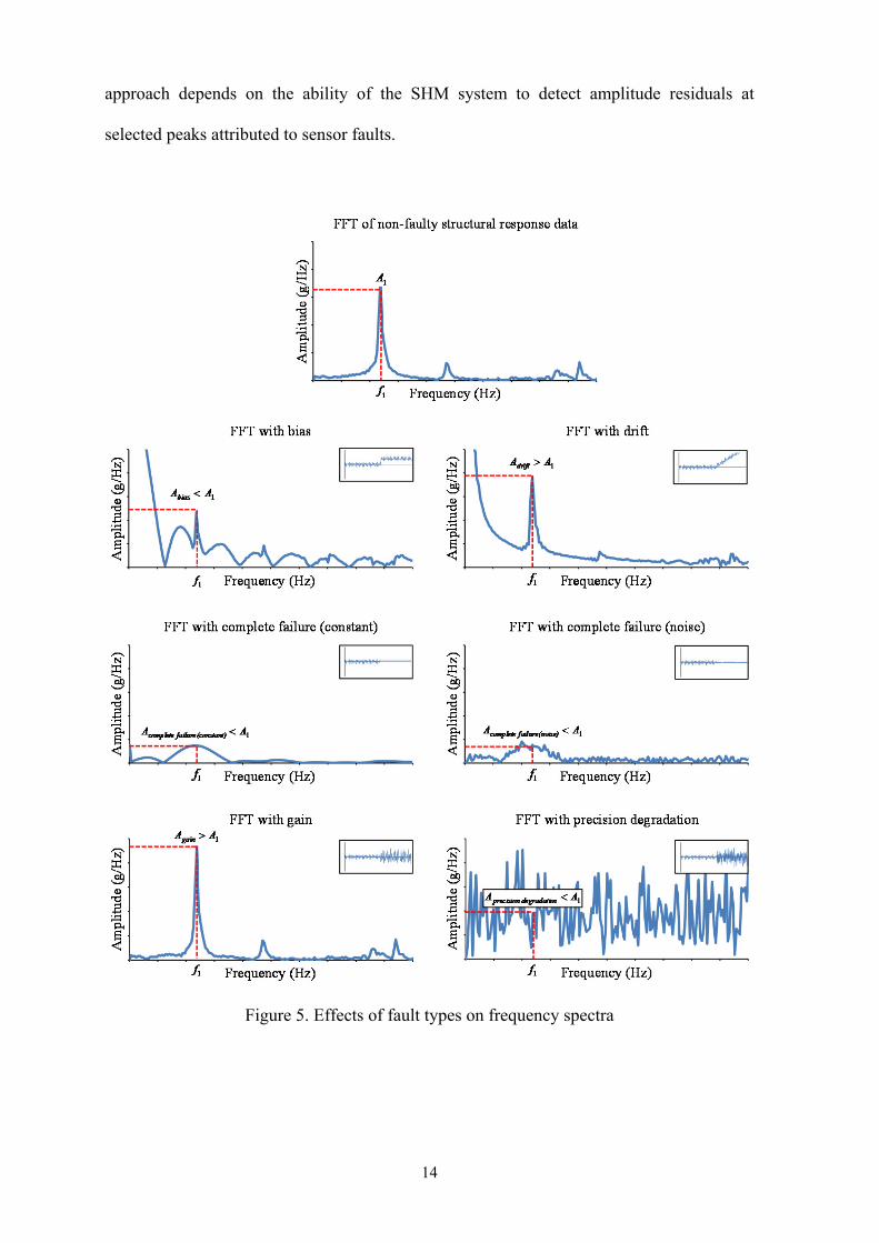
In general, all fault types have an effect on the frequency spectrum. Figure 5 shows how

the frequency spectrum of a response data set is affected if the faults shown in Figure 4

occur. While the impact of each fault on the general shape of the spectrum is obvious, it

should be noted that the dependability and accuracy of the fault diagnosis approach

described in this paper depends on the effect of the fault on the amplitudes of the selected

peaks. It is not uncommon that sensor faults introduce spurious components into the

frequency spectrum and contaminate the overall frequency content of the signal. However,

if the effect on the amplitude at the selected peaks is low, the difference between the

expected (i.e. predicted) Fourier amplitude and the actual Fourier amplitude could be small

and the fault could be therefore undetectable. Hence, the efficiency of the fault diagnosis

btftf ˆ

Bias

Sens

or o

utpu

t

Time

btf ˆ

(constant) failure Complete

Sens

or o

utpu

t

Time

0,ˆ

Gain Rbtfbtf

Sens

or o

utpu

t

Time

tbtftf ˆ

Drift

Sen

sor

outp

ut

Time

2,0~,ˆ

(noise)failureComplete

Ntwtwtf

Sens

or o

utpu

t

Time

2,0~,ˆ

ndegradatioPrecision

Ntwtwtftf

Sen

sor

outp

ut

Time

14

approach depends on the ability of the SHM system to detect amplitude residuals at

selected peaks attributed to sensor faults.

Figure 5. Effects of fault types on frequency spectra

15

2.3 Implementation of the fault diagnosis methodology

The distributed analytical redundancy approach is implemented into a fault-tolerant

wireless SHM system prototype. The SHM system is composed of (i) wireless sensor

nodes installed in the monitored structure, (ii) a base station, and (iii) a server with data

storage and data analysis capabilities. The prototype SHM system supports the following

monitoring tasks, as shown in Figure 6: 1) data acquisition, 2) data processing, 3) fault

diagnosis, 4) data transmission, 5) data storage, and 6) data analysis. Data acquisition and

data processing are performed on-board the sensor nodes by transforming the acceleration

response data of the structure from the time domain into the frequency domain using a

Cooley-Tukey fast Fourier transform algorithm. A peak detection algorithm is executed to

identify the highest peak and the corresponding frequency (fundamental eigenfrequency of

the structure). Fault diagnosis is performed by the wireless sensor nodes in a distributed-

collaborative manner. The results of the fault diagnosis are wirelessly communicated

through the base station to the host computer for decision making. The data is eventually

analyzed, using various software tools on the host computer.

Figure 6. Monitoring tasks supported by the fault-tolerant wireless SHM system

16

2.3.1 Distributed adaptive fault diagnosis

The following discussion focuses on the “fault diagnosis” monitoring task and the

embedded software designed for distributed autonomous fault diagnosis. Representing a

distinct advantage of the analytical redundancy approach, no prior knowledge about the

characteristics of the monitored structure is required for performing fault diagnosis,

because an entirely data-driven approach is proposed. To this end, machine learning

algorithms that implement ANNs (Fiesler and Beale, 1997) are employed for the prediction

of the expected Fourier amplitudes of the sensor nodes, taken as the basis for fault

diagnosis.

The ANNs embedded into each sensor node comprise several neurons structured in three

layers (Figure 7). Figure 7 shows the topology of an ANN embedded into sensor node j. In

the input layer of the ANN, the actual Fourier amplitudes of k correlated sensor nodes of

the wireless SHM system are entered upon wireless receipt from the adjacent sensor nodes

1…k (“inputs”). The output layer contains one neuron that predicts the expected Fourier

amplitude of sensor node j (“output”). To account for the nonlinear relationship between

the inputs and the output, drawing from ANN theory, the hidden layer of m neurons is

devised to link the input layer with the output layer. The connections between the neurons,

the “synapses”, are used for data exchange between the neurons. The training of the ANNs

is achieved by adjusting the weights of the synapses until a set of input Fourier amplitudes,

taken from training data obtained in preliminary laboratory tests, results in the desired

Fourier amplitude of sensor node j. Finally, the properties of the ANN are determined.

ANN properties essentially encompass the network topology (such as the number of

neurons per layer) and the neuron behavior (such as the functions used to link the output of

17

one neuron to the input of the subsequent neuron).

Figure 7. Artificial neural network embedded into sensor node j

The size of the implemented ANN needs to be kept as small as possible to preserve the

limited computational resources of the sensor nodes. Hence, in each ANN only a limited

number of sensor nodes are considered. In large SHM systems, the sensor nodes are

divided in clusters, and one ANN is implemented in each cluster, thus maintaining a

reduced size for the ANNs.

2.3.2 Embedded software architecture

To implement the fault diagnosis methodology, software is written in Java programming

language, exploiting the merits of object-orientation and platform independence. The

software consists of two packages, the sensornode package (executed on the sensor

nodes) and the basestation package (executed on the host computer). Every package

includes several Java classes, used as “blueprints”, from which individual Java objects are

created, representing the real-world objects relevant to SHM.

18

As illustrated in the class diagram shown in Figure 8, the package sensornode contains

Java classes designed for data acquisition, data processing, fault diagnosis (i.e. training and

operating the ANNs), and data communication (AccelerationSampler, FFT,

Sample, NetworkTraining, Communication, and MainNode). In addition,

several classes are imported into the package from an external library, the SNIPE library,

that supports the implementation of artificial neural networks (Kriesel, 2010). The entry

point of the overall SHM application, which starts the operation of the sensor nodes, is the

startApp() method in the MainNode class. In the MainNode class, instances of the

AccelerationSampler class, of the FFT class, of the NetworkTraining class, of

the Communication class, and of the SNIPE neural network classes are created to

autonomously perform the monitoring tasks, including fault diagnosis. Specifically, the

AccelerationSampler class is designed for measuring the acceleration of the

monitored structure. The measured values are stored in an array on the sensor nodes. The

FFT class performs an FFT according to the Cooley-Tukey algorithm to transform the

measured accelerations from the time domain into the frequency domain, followed by a

peak detection algorithm to provide insights into potential structural changes. The

information relevant to fault diagnosis, i.e. the Fourier amplitudes and the

eigenfrequencies, is packaged in the Sample class. The Sample class, in addition to the

amplitudes and the eigenfrequencies, also includes the address of the specific sensor node

as well as a Boolean value that indicates a sensor fault.

The basestation package, illustrated in Figure 9, handles the tasks of the host

computer; it includes the classes DatabaseHandler, MainBase, and Sample. The

MainBase class is designed to manage radio connections between the base station and the

sensor nodes; it also receives data sent by the sensor nodes and communicates with objects

19

of the DatabaseHandler class. The DatabaseHandler class establishes a

connection to a MySQL database installed on the host computer, automatically creates

database tables and inserts the data relevant to fault diagnosis, i.e. the results of the fault

diagnosis from each sensor node, into the database.

Figure 8. Class diagram of package “sensornode”

Figure 9. Class diagram of package “basestation”

3 Validation tests

Validation tests are devised to showcase the ability of the proposed approach to diagnose

sensor faults reliably and accurately as well as to demonstrate the adaptability of the

approach to changes in the structural condition. First, the properties of the ANN are

20

defined. Then, the fault diagnosis approach is applied and validated for two structural

conditions, initial and changed.

3.1 Hardware used

The sensor nodes and the base station used in this study are of type “Oracle Sun SPOT”

(Oracle Corp., 2009, 2010). Each sensor node includes a main board, a battery, and an

exchangeable application board. The outer dimensions of each sensor node are

41 mm × 70 mm × 23 mm (length × width × height), and the weight of each sensor node is

54 g. The main board features a Java-programmable 400 MHz ARM main processor, 1 MB

RAM, 8 MB flash memory and an IEEE 802.15.4 radio transceiver. The application board

includes a digital output accelerometer, an ambient light sensor, a temperature sensor, and

eight tricolor LEDs. The integrated accelerometer is of type MMA7455L with a selectable

measurement range between ± 2 g and ± 8 g.

3.2 Experimental setup

The wireless SHM system implemented to validate the proposed fault diagnosis approach

is installed on a test structure. The test structure is a 4-story frame structure consisting of

steel plates of 25 cm × 50 cm × 0.8 mm (length × width × thickness). The plates rest on steel

threaded rods with a story height of 23 cm. At the bottom of the structure, the rods are

fixed into a solid block of 40 cm × 60 cm × 30 cm. Figure 10 shows the instrumentation of

the test structure. The base station is connected to a server placed next to the structure.

Since this approach is based on output-only data processing techniques, the excitation of

the structure is performed by deflecting the top story from the equilibrium position without

21

measuring the excitation force.

Figure 10. Laboratory test set-up

3.3 Determination of the artificial neural network properties

The determination of suitable ANN properties is conducted in preliminary laboratory tests

that are executed prior to the actual validation tests. Since the ANNs embedded into the

sensor nodes are able to adapt to the condition of the monitored structure (i.e. on the

laboratory test structure), the ANN properties for the fault diagnosis approach are case-

specific, thus depending on the characteristics of the monitored structure and on the SHM

system setup. Different topologies and different neuron behaviors are implemented for test

purposes. The criteria employed for the definition of the ANN properties are related to the

performance of the ANN, i.e. the time needed to produce the output, and to the prediction

accuracy, i.e. the residuals between the expected Fourier amplitude and the actual Fourier

500.0

±0.00

+230

+460

+690

+920

-300

Elevationview

450.0

D1

D3

D2

Plan view

250.0

45.0

27.0

M5 steel threaded rodwith nut and washer

Steel plate(500x250x0.8)

M5 threadedplug (socket)

M5 planted part of M5steel rod (varies fordifferent columns)

M5 nut

M5 washer

4.50.7

Detail D1

Detail D2

Detail D3

22

amplitude.

The prediction accuracy is expressed through the root mean square errors εRMS between the

expected Fourier amplitude (Fexpected) and the actual Fourier amplitude (Factual) at the

fundamental eigenfrequency (ω1), calculated and averaged for all iterations (N), as shown

in Eq. 5.

N

FFN

iiactual,iexpected,

RMS

1

21

21

(5)

Using the test setup shown in Figure 10, data of three correlated sensor nodes is deployed

to feed the ANN of one sensor node; hence, each ANN has three input neurons and,

reflecting the expected Fourier amplitude to be predicted, one output neuron is required.

Between the input layers and the output layer, various numbers of hidden layers as well as

various hidden neurons per layer are tested. Interlayer connections, allowing only synapses

between neurons in adjacent layers, as well as supralayer connections, allowing synapses

between neurons in distant layers, are considered. As for the neuron behaviors, two

different training algorithms, the backpropagation algorithm and the resilient

backpropagation algorithm are tested (Rumelhart et al. 1986, Riedmiller & Braun 1993).

By exciting the test structure, a total of 100 acceleration response data sets is collected and

transformed into the frequency domain by the sensor nodes. The Fourier amplitude

corresponding to the fundamental eigenfrequency of the structure is computed on board the

sensor nodes, and both values (amplitude and frequency) are transmitted, through the base

station, to the database for storage. Following the general practice of neural network

23

applications, each data set is divided into three subsets, a training set, a validation set, and

a test set, which allows stopping the training process as soon as overfitting starts to occur.

The training set is used for adjusting the weights of the ANNs. The validation set is used to

monitor the training process, i.e., when the network begins to overfit the data, the error on

the validation set typically begins to rise. Thus, the network weights are saved at the

minimum error. The test set, being independent from the training set and the validation set,

is used to test the final solution to confirm the predictive power of the ANNs.

The results of the determination of the ANN properties are summarized in Table 1. In

general, all ANN topologies and neuron behaviors tested are capable of predicting Fourier

amplitudes for fault detection. The smallest root mean square errors, representing the best

results and thus the best prediction accuracy, are obtained with interlayer-connected

topologies and backpropagation (0.063 ≤ εRMS ≤ 0.144). Using topologies with supralayer

connections or the resilient backpropagation training algorithm leads to root mean square

errors between 0.132 and 0.208. Considering a reasonable trade-off based on the

performance criterion and the prediction accuracy criterion, a 3-2-1 interlayer-connected

ANN topology with backpropagation is determined to be ideal for the test structure used in

this study, thus being embedded into each sensor node for the validation tests.

24

Table 1. Prediction accuracy of the wireless SHM system

Neuron behavior Topology Neurons per sensor node

Computing time (s)

εRMS (-)

Interlayer, backpropagation

3-1 4 6.6 0.149 3-2-1 6 13.0 0.096 3-3-1 7 17.2 0.144 3-5-1 9 25.0 0.081 3-7-1 11 32.2 0.063 3-2-2-1 8 21.0 0.092 3-5-5-1 14 46.6 0.137

Interlayer and supralayer, backpropagation

3-3-1 7 15.2 0.147 3-5-1 9 22.6 0.132 3-2-2-1 8 19.4 0.137

Interlayer, resilient backpropagation

3-3-1 7 113.0 0.153 3-5-1 9 172.4 0.143 3-2-2-1 8 120.6 0.208

3.4 Operation of the SHM system

Implementing the ANNs with the previously determined properties into the fault-tolerant

wireless SHM system prototype, two validation tests are performed to validate the

efficiency and accuracy of the fault diagnosis approach. In the first validation test, sensor

faults are simulated to be detected by the SHM system. Since the embedded ANNs are

capable of adapting to the condition of the monitored structure, the second validation test is

devised to showcase the ability of the fault-tolerant SHM system to adapt to changes in the

condition of the monitored structure. Therefore, in the second validation test, the structural

condition is changed by introducing damage, and the same sensor faults as in the first test

are simulated to be detected once the SHM system has adapted to the changed condition.

3.4.1 Fault diagnosis at initial structural condition

The first validation test (test 1) is performed in the initial, i.e. undamaged, condition of the

25

structure. The simulation of two of the most common fault types, gain and complete

failure, is exemplarily shown in the following. Fixation issues, not uncommon in structural

health monitoring, are the most frequent sources of gain. Faulty sensors with gain are often

found to have sustained a partial loss of connectivity to the structure, which results in loss

of sensor orientation and in scaling of the collected response data. In this study, gain is

simulated by rotating the sensor node by an angle of 45o (Figure 11). Furthermore,

complete failure is manifested through either a constant value or noise in the sensor output

instead of the actual response. In this study, complete failure is simulated by substituting

the sensor outputs with random values.

A total of 30 acceleration response data sets, each containing 1024 data points, is collected.

Similar to the procedure towards determining the optimum ANN properties, fault diagnosis

is performed based on the root mean square error between the expected and actual Fourier

amplitudes, as shown in Eq. 5, which reflects the prediction accuracy of the approach.

Figure 11. Simulation of bias sensor fault type at sensor node B

26

To validate the distributed autonomous fault diagnosis, the test structure is excited by

deflecting the top story from the equilibrium position and by letting the structure to vibrate

freely. Upon collecting a preliminary response data set, the peak detection algorithm

embedded in each sensor node is executed to verify that the eigenfrequency used for

training of the ANNs has not been changed (i.e. no structural change has occurred). Once

the 30 response data sets are collected, the embedded ANN of sensor node B predicts the

expected Fourier amplitude of the sensor node using the Fourier amplitudes requested from

sensor nodes A, C, and D as input data. The actual Fourier amplitude of sensor node B is

computed via the embedded FFT algorithm. The residuals between the expected Fourier

amplitude and the actual Fourier amplitude are calculated and averaged over the 30 data

sets to extract the root mean square error. The fault detection is realized by comparing the

residuals to a fault threshold with εRMS < indicating non-faulty sensor operation. The

fault threshold is defined using the results from the test above as benchmarks and set to

τ = 0.15 derived from good engineering judgment. The results for both simulated sensor

fault types are summarized in Table 2.

Table 2. Distributed autonomous detection of sensor faults.

Root mean square error No fault Simulated fault

Gain Complete failureεRMS 0.102 0.264 0.372

As can be seen from Table 2, if no fault occurs in the SHM system, the root mean square

error is εRMS = 0.102 corresponding to the test set of the data set . A root mean square error

εRMS = 0.264 corresponds to the simulated gain fault, while in the case of complete failure,

the respective root mean square error is εRMS = 0.372. The increased values of εRMS indicate

the presence of faults as well as the efficient detection of sensor faults. Figure 12 shows

27

how the amplitudes of the peaks corresponding to the fundamental eigenfrequency are

affected by the faults considered in this study.

Figure 12. Comparison of frequency spectra between non-faulty operation (left), bias fault

(middle), and precision degradation fault (right).

3.4.2 Fault diagnosis at changed structural condition

An important ability of the analytical redundancy approach is to adapt to changes in the

structural condition. Hence, the second validation test is conducted after damage is

introduced to the structure, considering a change in the structural condition affecting the

simulated sensor faults. The damage is introduced by loosening the column-to-plate

connections on one side of the structure, as shown in Figure 13.

050

100150200250

0 20 40

Am

plitu

de (

g/H

z)

Frequency (Hz)

FFT with non-faulty response data

050

100150200250

0 20 40A

mpl

itude

(g/

Hz)

Frequency (Hz)

FFT with gain

050

100150200250

0 20 40

Am

plit

ude

(g/H

z)

Frequency (Hz)

FFT with complete failure (noise)

28

Figure 13. Damage introduced to the test structure

The same fault types as in the validation test 1 are considered. The structure is deflected at

the top story and left to vibrate freely. A preliminary response data set is collected and the

peak detection algorithm is executed to investigate whether a change in the frequency of

the highest peak has occurred; structural changes are followed by a shift of the peaks in the

Fourier spectrum, and once this shift is identified by the SHM system, a beacon signal is

sent to the server to request the retraining of the ANNs. Upon completion of the ANN

retraining (adaptation), 30 response data sets are collected and the same procedure as in

validation test 1 is followed. The expected Fourier amplitude of node B is predicted by the

ANN using the amplitudes of nodes A, C, and D as input data. The actual amplitude of

node B is then computed by the embedded FFT algorithm and the residual between the

expected and actual Fourier amplitudes is calculated and averaged for the 30 data sets,

being adapted to the changed (damaged) structural condition.

29

4. Summary and conclusions

Efficient and accurate sensor fault diagnosis is paramount for ensuring the reliability and

consistency of structural health monitoring (SHM) systems. To date, most fault diagnosis

approaches are based on the centralized storage of data on a server, where the data is

analyzed in order to detect and isolate sensor faults. However, centralized fault diagnosis

requires considerable data transfer, which in the case of wireless SHM systems is highly

power consuming. Approaches towards decentralized fault diagnosis for wireless SHM

system may eliminate the need for centralized collection of data, but the embedded

algorithms used rely on the wireless communication of raw data, thus still posing a non-

negligible operational constraint due to the limited power resources of wireless sensor

nodes. The exploitation of the embedded computing capabilities of wireless sensor nodes

in terms of on-board data processing for fault diagnosis has received little attention. In this

paper, a distributed approach towards autonomous fault diagnosis has been presented using

the concept of analytical redundancy. Abnormal sensor outputs are detected based on the

inherent correlations among the Fourier amplitudes of structural response data from

different sensors at peaks corresponding to the eigenfrequencies of the structure. The

approach proposed in this study is entirely data-driven requiring no a priori knowledge of

the structure or of the SHM system. Fault diagnosis is performed by calculating the

deviation between the actual Fourier amplitudes of measured acceleration response data

and the expected Fourier amplitudes predicted from the sensor outputs of correlated sensor

nodes. The expected Fourier amplitudes of each sensor node are predicted by embedded

artificial neural networks taking into account the actual condition of the monitored

structure. By communicating only the Fourier amplitude at selected peaks, fault diagnosis

is performed with minimal data traffic, thus preserving the limited power resources of

30

wireless sensor nodes.

The distributed analytical redundancy approach has been validated through laboratory tests

on a 4-story frame structure. The fault diagnosis methodology has been implemented into a

wireless SHM system, which has been installed on the frame structure. Suitable properties,

i.e. topology and neuron behavior, of the ANN for implementing the proposed approach

into the laboratory test structure have been determined based on the performance and the

prediction accuracy of the ANN output. Based on the aforementioned criteria, a 3-2-1

ANN topology (3 input layers, 2 hidden layers, one output layer) and backpropagation

neuron behavior has been identified as the ideal topology for the wireless SHM system

employed in the present study. The selected ANN topology has been embedded into the

sensor nodes, and two validation tests have been performed. Test 1 has been conducted in

the initial structural condition with non-faulty sensors, while test 2 has been conducted

with faulty sensors and after inducing structural changes (i.e. damage). The results of the

validation tests clearly demonstrate the ability of the proposed approach to diagnose sensor

faults efficiently and accurately, as well as the ability of the ANNs to adapt to structural

changes. It is clear that the efficiency and accuracy of the fault diagnosis depends on the

impact of the fault on the amplitudes of the selected peaks of the Fourier spectrum.

Therefore, future research will focus on investigating the applicability limits of the

proposed approach with respect to different sensor fault types, which have different impact

on the frequency content of the structural response.

Acknowledgements

The authors would like to gratefully acknowledge the support offered by the German

31

Research Foundation (DFG) under grant GRK 1462 (“Evaluation of Coupled Numerical

and Experimental Partial Models in Structural Engineering”). The financial support is

gratefully acknowledged. The authors would like to extend their gratitude to Mrs. Katrin

Jahr, who has developed parts of this work at the Chair of Computing in Civil Engineering

at Bauhaus University Weimar. Any opinions, findings, conclusions or recommendations

expressed in this paper are those of the authors and do not necessarily reflect the views of

DFG.

References

Basirat, A. H. and Khan, A. I. (2009). “Graph neuron and hierarchical graph neuron, novel

approaches toward real time pattern recognition in wireless sensor networks”. In: Proc. of

the 2009 International Conference on Wireless Communications and Mobile Computing.

Leipzig, Germany, 21/06/2009.

Benedettini, O., Baines, T. S., Lightfoot, H. and Greenough, R. M. (2009). “State-of-the-

art in integrated vehicle health management”. Journal of Aerospace Engineering, Vol. 223,

No. 2, pp. 157-170.

Bisby, L. A. (2014). “An introduction to structural health monitoring”. ISIS Educational

Module 5, Queen’s University ,Toronto, ON, Canada, 2014.

Brincker, R., Andersen, P. and Zhang, L. (2000). “Modal identification from ambient

responses using frequency domain decomposition”. In: Proc. of the 18th International

Modal Analysis Conference (IMAC), San Antonio, TX, USA, 07/02/2000.

32

Cho, S., Yun, C. B., Lynch, J. P., Zimmerman, A., Spencer, Jr. B. and Nagayama, T.

(2008). “Smart wireless sensor technology for structural health monitoring”. Steel

Structures, Vol. 8, No. 4, pp. 267-275.

Cooley, J. W. and Tukey, J. W. (1965). “An algorithm for the machine calculation of

complex Fourier series”. Mathematics of Computation, Vol. 19, No. 90, pp. 297-301.

Doebling, S., Farrar, C., Prime, M. and Shevitz, D. (1996). “Damage identification and

health monitoring of structural and mechanical systems from changes in their vibration

characteristics: a literature review”. Technical report No: LA-13070-MS, Los Alamos

National Lab., NM, USA, 1996.

Dragos, K. and Smarsly, K. (2015). “A comparative review of wireless sensor nodes for

structural health monitoring”. In: Proc. of the 7th International Conference on Structural

Health Monitoring of Intelligent Infrastructure. Turin, Italy, 01/07/2015.

Frank, P. M. (1990). “Fault diagnosis in dynamic systems using analytical and knowledge-

based redundancy”. Automatica, Vol. 26, pp. 459-474.

Fiesler, E. and Beale, R. (1997). “Handbook of neural computation”. Oxford University

Press, Oxford, UK, 1997.

Hitt, E. F. and Mulcare, D. (2001). “Fault-Tolerant Avionics”. The Avionics Handbook, C.

R. Spitzer (eds.), Taylor & Francis Group, London, UK, 2001.

Isermann, R. (2005). “Model-based fault-detection and diagnosis – status and

33

applications”. Annual Reviews in Control, Vol. 29, No. 1, pp. 71-85.

Isermann, R. (1984). “Process fault-detection based on modelling and estimation methods

– a survey”. Automatica, Vol. 20, pp. 387-404.

Jahr, K., Schlich, R., Dragos, K. and Smarsly, K. (2015). “Decentralized autonomous fault

detection in wireless structural health monitoring systems using structural response data”.

In Proc. of the 20th International Conference on the Applications of Computer Science and

Mathematics in Architecture and Civil Engineering (IKM). Weimar, Germany, 22/07/2015.

Kane, M., Zhu, D., Hirose, M., Dong, X., Winter, B., Häckel, M., Lynch, J. P., Wang, Y.

and Swartz, A. (2014). “Development of an extensible dual-core wireless sensing node for

cyber-physical systems”. In: Proc. of SPIE, Sensors and Smart Structures Technologies for

Civil, Mechanical, and Aerospace Systems, San Diego, CA, USA, 09/03/2014.

Kraemer, P. and Fritzen, C.-P. (2007). “Sensor Fault Identification Using Autoregressive

Models and the Mutual Information Concept”. Key Engineering Materials, Vol. 347, pp.

387-392.

Kriesel, D. (2007). “A brief introduction to neural networks”. Available at:

http://www.dkriesel.com.

Kullaa, J. (2010). “Detection, identification, and quantification of sensor fault”. In: Proc.

of 24th International Conference on Noise and Vibration engineering (ISMA2010),

Leuven, Belgium, 20/09/2010.

Lei, Y., Shen, W. A., Song, Y. and Wang, Y. (2010). “Intelligent wireless sensors with

application to the identification of structural modal parameters and steel cable forces: from

the lab to the field”. Advances in Civil Engineering, Vol. 2010, pp.1-10.

34

Lynch, J. P., Sundararajan, A., Law, K. H., Sohn, H. and Farrar, C. R. (2004). “Design of a

wireless active sensing unit for structural health monitoring”. In: Proc. of SPIE’s 11th

Annual Int. Symposium on Smart Structures and Materials, San Diego, CA, USA,

14/03/2004.

Mehrotra, K., Mohan, C. K. and Ranka, S. (1997). “Elements of artificial neural

networks”. MIT press, Cambridge, MA, USA, 1997.

Moore, E. F. and Shannon, C. E. (1956). “Reliable circuits using less reliable relays”.

Journal of the Franklin Institute, Vol. 262, No. 3, pp. 191-208.

Obst, O. (2009). “Distributed fault detection using a recurrent neural network”. In:

Proceedings of the 2009 International Conference on Information Processing in Sensor

Networks. Washington, DC, USA, 13/04/2009.

Olney, P. and Morgenthal, G. (2015). “Simulating sensor attributes to quantify the utility

of monitoring systems”. In: Proc. of the 7th International Conference on Structural Health

Monitoring of Intelligent Infrastructure, Turin, Italy, 01/07/2015.

Oracle Corp. (2009). “Sun SPOT Theory of Operation, 1.5.0”. Sun Labs, Santa Clara, CA,

USA, 2009.

Oracle Corp. (2010). “Sun SPOT eDEMO Technical Datasheet, 8th edition”. Sun Labs,

Santa Clara, CA, USA, 2010.

35

Qin, S. J. and Li, W. (1999). “Detection, identification, and reconstruction of faulty sensors

with maximized sensitivity”. Journal of American Institute of Chemical Engineers, Vol.

45, No. 9, pp. 1963-1976.

Richardson, M. H. and McHargue, P. L. (1993). “Operating deflection shapes from time

versus frequency domain measurements”. In: Proc. of IMAC-XI, International Modal

Analysis Conference and Exposition. Kissimmee, Orlando, FL, USA, 01/02/1993.

Patton, R. J. (1990). “Fault detection and diagnosis in aerospace systems using analytical

redundancy”. In: Proc. of the IEE Colloquium Condition Monitoring and Fault Tolerance.

London, UK, 11/06/1990.

Patton, R. J., Frank, P. M. and Clark, P. N. (2000). “Issues of fault diagnosis for dynamic

systems”. Springer Publishing, Berlin, Germany, 2000.

Rajakarunakaran, S., Venkumar, P., Devaraj, D. and Rao, K. (2008). “Artificial neural

network approach for fault detection in rotary system”. Applied Soft Computing, Vol. 8,

No. 1, pp. 740-748.

Riedmiller, M. and Braun, H. (1993). “A direct adaptive method for faster backpropagation

learning: The RPROP algorithm”. In: Proc. of the IEEE International Conference on

Neural Networks, San Francisco, CA, 28/03/1993.

Rumelhart, D. E., Hinton, G. E. and Williams, R. J. (1986). “Learning representations by

back-propagating errors”. Nature, Vol. 323, pp. 533-536.

36

Salawu, O.S. (1997). “Detection of structural damage through changes in frequency: a

review”. Engineering structures, Vol. 19, No. 9, pp. 718-723.

Smarsly, K. (2014). “Fault diagnosis of wireless structural health monitoring systems

based on online learning neural approximators”. In: Proc. of the International Scientific

Conference of the Moscow State University of Civil Engineering (MGSU). Moscow,

Russia, 11/12/2014.

Smarsly, K. and Law, K. H. (2013). “A migration-based approach towards resource-

efficient wireless structural health monitoring”. Advanced Engineering Informatics, Vol.

27, No. 4, pp. 625-635.

Smarsly, K. and Petryna, Y. (2014). “A Decentralized Approach towards Autonomous

Fault Detection in Wireless Structural Health Monitoring Systems”. In: Proc. of the 7th

European Workshop on Structural Health Monitoring. Nantes, France, 08/07/2014.

Smarsly, K. and Law, K. H. (2014). “Decentralized fault detection and isolation in wireless

structural health monitoring systems using analytical redundancy”. Advances in

Engineering Software, Vol. 73, pp. 1-10.

Smith, S. W. (1999). “The Scientist and Engineer's Guide to Digital Signal Processing

(second edition)”. California Technical Publishing, San Diego, CA, USA, 1999.

Venkatasubramanian, V., Vaidyanathan, R. and Yamamoto, Y. (1990). “Process fault

detection and diagnosis using neural networks – 1. Steady-state processes”. Computers &

Chemical Engineering, Vol. 14, No. 7, pp. 699-712.

Von Neumann, J. (1956). “Probabilistic logics and the synthesis of reliable organisms from

unreliable components”. Automata Studies, Princeton, NJ, USA, Shannon, C. E.,

37

McCarthy, J., pp. 329-378.

Wang, Y., Lynch, J. P. and Law, K. H. (2007). “A wireless structural health monitoring

system with multithreaded sensing devices: Design and validation”. Structure and

Infrastructure Engineering, Vol. 3, No. 2, pp. 103-120.

Willsky, A. S. (1976). “A survey of design methods for failure detection systems”.

Automatica, Vol. 12, pp. 601-611.

Yuen, K.-V. and Lam, H.-F. (2006). “On the complexity of artificial neural networks for

smart structures monitoring”. Engineering Structures, Vol. 28, No. 7, pp. 977-984.

Zimmerman, A., Shiraishi, M., Schwartz, A. and Lynch, J. P. (2008). “Automated modal

parameter estimation by parallel processing within wireless monitoring systems”. ASCE

Journal of Infrastructure Systems, Vol. 14, No. 1, pp. 102-113.