basic quantum mechanics prof. ajoy ghatak department of...

Basic Quantum Mechanics Prof. Ajoy Ghatak

Department of Physics Indian Institute of Technology, Delhi

Module No. # 07

Bra-Ket Algebra and Linear Harmonic Oscillator - II Lecture No. # 01

Dirac’s Bra and Ket Algebra

Immediately, after Schrodinger and before that Heisenberg wrote down the papers on

quantum mechanics, after about a year or so, Dirac presented his own formalism of

quantum mechanics and very soon, he published, one of the classic texts on quantum

mechanics. He introduced the Bra and Ket algebra and also provided a very elegant, an

extremely elegant formulation of quantum mechanics. We will continue our discussions

on this formulism.

(Refer Slide Time: 01:20)

However, before that I thought, I will mention that Albert Einstein, who is regarded as

one of the most outstanding physicists of all times had said about Dirac’s work that,

“Dirac, to whom in my opinion, we owe the most logically perfect presentation of

quantum mechanics.” This I have quoted from a book by Professor Mukunda, in which

he made this quotation. So, Dirac’s formalism of quantum mechanics is as according to

Einstein, is the most logically perfect presentation of quantum mechanics.


The references will be, of course, the classic text of this subject is Professor Dirac’s

book, which is entitled as, “Principles of Quantum Mechanics” and published by Oxford

University Press and I think in 1958, it was the 4th edition of his famous book.

The book came out just after in the late 1920s actually. We have, as I have been

mentioning, our own book on quantum mechanics and in which, we have given the

formulation that I will be following in this and the following lectures. There is also a

very nice book by J Townsend and actually the title of the book is, “The Modern

Approach to Quantum Mechanics” and is published by McGraw Hill in 1992.

Of course, there are many numerous books. There is a book by Gordon Beam and of

course, the Feynman lectures on physics, volume 3, and I will advice all of you to go to

that the Feynman lectures volume 3. So, we consider the dynamical system and a

dynamical system can be a linear harmonic oscillator, or just an electron, or a hydrogen

atom, or a diatomic molecule or something like that. Now, each state of the dynamical

system can be represented by a certain type of vector.


By certain type of ket vector, which we write like this, and in order to distinguish it from

other vectors, we put a symbol, so that a state of a dynamical system can be represented

by a ket vector, which is known as the ket vector and which forms a dual vector space.

The vector space is linear, in the sense that if we have another vector B, then another ket

vector B, then the linear combination C 1 A plus C 2 B where C 1 and C 2 are complex

numbers is also a vector in the same space.


Now, I will quote from Professor Dirac’s book on quantum mechanics and let us read

this through. If you want to read the original quotation, which of course, is given in his

book, but let us read this through slowly. “Each state of a dynamical system at a

particular time corresponds to a ket vector, the correspondence being such that if a state

results from the superposition of certain other states, its corresponding ket vector is

expressible linearly in terms of the corresponding ket vectors of the other states, and

conversely.”

So, this is introduced in a slightly abstract manner, but we hope, we will get a physical

understanding of this shortly.


Then it is a dual vector space, dual vector space, so that corresponding to the ket A there

is a unique bra A, and then a corresponding to ket B there is a bra B, such that bra A ket

B is a complex number, c number; c number means, it is a complex number. This

quantity is known as the scalar product of the vector A with vector B, and is such, this is

axiom, which means something like an assumption; there is no proof of this. So,

according to this axiom, the complex conjugate of this number is equal to B A.

If A A 1, sorry, If A B 1 is equal to A B 2, for any ket vector A, for any bra A, then we

say that B 1 is equal to B 2. Similarly, if A 1 B is equal to A 2 B, for any ket, for an

arbitrary ket B, then we say that bra A 1 is equal to bra A 2. So, the equality is through

the scalar product. Similarly, if bra A ket B is 0, is a null ket for any bra A, then ket B is

said to be a null ket. Similarly, if bra A ket B is 0 for any ket B then bra is A null bra.


Similarly, if I have A, A and if this is 1, then the ket A is said to be normalized. Now, we

had said that A B, the complex conjugate of that is equal to B A. So, if B is A that is if

ket B is equal to A, then bra B is equal to bra A, then I can write down that A A bar is

equal to A A, so that this quantity is real.

We further assert this also. We further assert that bra A ket A is always a positive

definite, equal to 0, if and only if, ket A is a null ket. So, if the scalar product of a ket

with its own bra is always positive, if it is 0, then ket A must be A null ket and bra A,

corresponding bra A will be also a null bra. Now, if I have, this is the linearity relation, if

I had P is equal to C 1 A plus C 2 B, then bra P is equal to C 1 star; this is a complex

number, C 1 star bra A plus C 2 star bra B (Refer Slide Time: 11:29). This is the linearity

relation.

As I had mentioned yesterday, if ket A corresponds to a state, whose wave function is

given by, say psi of r in the Schrodinger representation, and if bra B ket B is represented

by the state, which is represented by the wave function phi, the corresponding ket vector

is B, the state of this system or of the harmonic oscillator or of the hydrogen atom is

given by psi of r, and if its ket vector is denoted by A, then the relationship is through the

scalar product and that is B A will be equal to phi star psi d tau, integrated over the entire

space. So, this is the scalar product. (No Volume Between: 12:55-13:05)


Finally, if A B is 0, if this is a 0 number, then these two kets are said to be orthogonal to

each other. Now, let me just to make thing simple, let me consider the 2-dimensional

space. We can consider a 3 dimensional space also or a 4 dimensional space. But, just for

the sake of simplicity, we have, let us suppose ket A is represented by say 1 i.

Then bra A; let me put a 1 over under root 2 (Refer Slide Time: 14:04) and will be equal

to 1 over root 2 and this will be the corresponding. In order to understand, the Bra Ket

algebra, one can consider examples from theory of matrices and then everything

becomes clear. So, you have bra A ket A, will be equal to 1 over root 2, 1 minus i, 1, i.

So, this is 1 times 1 is 1, 1 over root 2 times 1 over root 2, so this is 1 over root 2 whole

square, so that is 1 over 2.

This becomes 1 over 2 into 2, so this is 1. So, it is a normalized ket. Similarly, if I

consider a bra B ket B and let us suppose, 1 over root 2, 1 minus 1. Then bra A ket B will

be equal to (bra A is 1 over root 2 times 1 over root 2 is) half and then 1 minus i, 1 minus

i. So, this is 1, minus into minus is plus, i square is minus 1, so 1 minus 1 is 0.

We say that these two kets, the A and B are orthogonal. We say that A and B are

orthogonal or are orthogonal vectors. We can consider another example in 3-dimensional

space.


Let us suppose in a 3-dimensional space, we write A is equal to 1 0 0, and B is equal to 0

1 0. Both of them have unit length, because bra A ket A will be 1 0 0, 1 0 0 and this will

be just 1. Similarly, ket B is also a normalized ket, but bra A ket B will be equal to 0.

This is how we understand. Let us consider and go back to a 2-dimensional space and let

us suppose A is equal to a, b, where a and b are complex numbers. So, then bra A will be

equal to a star, b star. It is a dual vector space. So, corresponding to every column vector

there is a row vector. So, bra A ket A will be a, a star and that is mod a square plus mod

b square and if this is 0, then a must be 0 and b must be 0.

In fact, if the scalar product is 0, so then a must be equal to 0 0. This is a null ket,

because you consider any bra B, say c, d. If I write down bra B ket A, so this will be,

sorry, this is bra B (Refer Slide Time: 18:09), this will be bra B and this will be c, d, 0, 0.

So, this is 0; this is a null ket, a null vector in a 2 dimensional space. You can consider a

3 dimensional space or a 4 dimensional space and so on.


Now, as we know that in the theory of matrices one vector, let us suppose, I consider a 2

dimensional vector 1, 1. If I multiply this by a vector like this, a square matrix like this, it

transforms to another vector. Let us suppose or let me put it like this as 1, 1, 1, 1, so this

becomes… This is not a good example, because… Let me redo the example. So, we have

here, for example, say (1, 2, 1, 2) and this is let us suppose 1 and 4.

So, this operating on that; this will be 1 times 1 is 1, 2 plus 4 is 6, and it finally gives us 9

and 6. So, a square matrix operating on a vector transforms to another vector. We say

that we consider a linear operator alpha, which if operates on A, it transforms to another

vector B, and this transformation is linear. Linear meaning that alpha is something like A

plus C, let us suppose, this is equal to alpha operating on A plus alpha operating on C.

So, it is a linear operator.

I can have alpha as a linear operator, alpha operating on C 1 A 1, plus C 2 A 2, plus C 3

A 3 where C 1, C 2, C 3 are all constants, are all complex numbers, then this is equal to

C 1 alpha A 1, plus C 2 alpha A 2, plus C 3 alpha A 3, etcetera. So, this is a consequence

of the linearity.


Then we say that two operators like the alpha and beta are said to be equal, if and only if,

I write two f’s here, that means if and only if, alpha A is scalar product is equal to B

alpha A. sorry sorry A alpha A for any ket A, I am sorry, this is A beta A (Refer Slide

Time: 22:15). If I consider two linear operators alpha and beta, and if this equality holds

for any ket vector A, then we say that alpha and beta are equal. If alpha operating on ket

A is a multiple of ket A, then we say that ket A is an eigen ket of the operator alpha,

belonging to the eigen value c, which in general can be complex.

This equation, when an operator operating on a ket, gives you a multiple of the same ket,

then this equation is known as an eigen value equation. I will give you an example. Let

me consider this 0, 1, 1, 0 (Refer Slide Time: 23:49). Now, if I multiply this, if I operate

this on 1 and 2, let us suppose. Then you can see 0 times 1 is 0, 1 times 2 is 2 and 1 times

1 is 1.

You see this is not a multiple of this (Refer Slide Time: 24:18). So, this is not an eigen

value equation. On the other hand, if I write like this (0, 1, 1, 0); operating on 1 and

minus 1. So, we get 0 times 1 is 1, 1 times minus 1 is minus 1, 1 times 1 is 1. This ket is

a multiple of this ket. In fact the multiplication constant is minus 1, so this is an eigen

value equation, 1 minus 1 is an eigen vector of this square matrix and the eigen value is

minus 1.

Let me take another example such as (0, 1, 1, 0); if I operate this on 1, 1, then I will get

1, 1. So, the eigen value is plus 1. So, this is not an eigen value equation and so 1, 2 is

not an eigen vector of this equation. But, 1, 1 and 1 minus 1, as you must have read from

your theory of matrices are both the eigen vectors of the operator (( )).

Finally, if the operator alpha operating on a ket vector produces a multiple of a ket

vector, then we say that this represents an eigen value equation.


We next define the adjoint of the operator alpha and we denote this adjoint, following

Dirac’s notation, by alpha bar. This is defined like this. So, the definition is through this

equation, but A alpha bar B, you see if I know this scalar product for any bra A or any

ket B, then I know alpha bar.

And this, by definition, is equal to in the reverse order B alpha A, which is a complex

number, and is this (Refer Slide Time: 27:39). So, let me calculate the adjoint of alpha

bar. So, let me put this as beta, so my beta bar, the adjoint of alpha bar is beta bar, which

is alpha bar bar. So, write down A alpha bar bar B, and let us do this carefully. This is

equal to A beta bar B. So, the adjoint of that is.

The definition of beta bar is B beta A, complex conjugate of that. But, beta is alpha bar,

so you get B alpha bar A, and then this by definition of alpha bar, is A alpha B bar bar.

This is a complex number, this is the scalar product, which is a number and the complex

conjugate of the complex conjugate is the number itself.

So, this is equal to A alpha B, because the complex conjugate of that is which is single

bar, and the complex conjugate of that of the complex conjugate, will be the same

number. Therefore, alpha bar bar, we proved and must be equal to alpha. So, the adjoint

of the adjoint of the operator alpha is always is the same operator. Now let me do more

little more algebra.


Let us define alpha ket A and let alpha ket A be equal to ket P. You just have to revise

this once or twice and then you will be able to get the hang of it and we will then work

out an example or 1 or 2 examples, then things will become straight forward. So, I take

A alpha bar B, is equal to, from the definition of alpha bar, B alpha A with A bar.

But alpha operating on A is ket P, so this is B P, a complex conjugate of that. From the

definition that we had introduced in the first slide, we have said that this is equal to P B

and therefore, since this holds for any ket B. Therefore, A alpha bar must be equal to bra

P. Therefore, if I have if I have ket P is equal to alpha A, then bra P is equal to A alpha

bar; a relation that you must remember.

We next try to find out what is the adjoint of the product of two operators? So, let me

write down this alpha beta. Let us suppose, I write this as alpha beta bar, so alpha beta

bar, say bra A ket B is equal to bra B alpha beta B. Sorry, this will be A (Refer Slide

Time: 33:13). Now, let me define ket P which is equal to beta A, so this is B alpha ket P.

So, if I reverse this, I will get bra P, alpha bar ket B. But, bra P is equal to A beta bar and

that is just now we have proved. Therefore, this will be bra A beta bar alpha bar. So, we

get the important result that alpha beta bar, the adjoint of the product is equal to the

product of the adjoint in the reverse order. In general, alpha beta is not equal to beta

alpha. They need not commute.

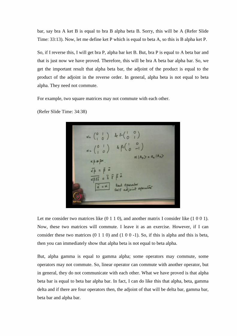
For example, two square matrices may not commute with each other.


Let me consider two matrices like (0 1 1 0), and another matrix I consider like (1 0 0 1).

Now, these two matrices will commute. I leave it as an exercise. However, if I can

consider these two matrices (0 1 1 0) and (1 0 0 -1). So, if this is alpha and this is beta,

then you can immediately show that alpha beta is not equal to beta alpha.

But, alpha gamma is equal to gamma alpha; some operators may commute, some

operators may not commute. So, linear operator can commute with another operator, but

in general, they do not communicate with each other. What we have proved is that alpha

beta bar is equal to beta bar alpha bar. In fact, I can do like this that alpha, beta, gamma

delta and if there are four operators then, the adjoint of that will be delta bar, gamma bar,

beta bar and alpha bar.

The adjoint of the product is the product of the adjoint, in reverse order. If alpha bar is

equal to alpha and if the adjoint of the operator is equal to the operator itself, then the

operator is said to be a real operator or this also known as a self adjoint operator or some

people call it as a Hermitian operator. So, if the adjoint is equal to the original operator

then we say that the operator is a real operator or a self adjoint operator. What I am going

to prove now is that if I write down the eigen value equation of the operator alpha then

alpha A n is equal to a n A n.


The eigen value equation of the operator alpha is given by alpha ket A n is equal to a n

ket A n. But, this is a number. This is a number and I write this sign as c number; c

number means, it can be a complex number, but we would show that if alpha bar is equal

to alpha, then a n must be real.

How do I show this? If this is ket P then you will have bra P is equal to bra A n alpha

bar, but alpha bar is equal to alpha, and this will be leave some space here. So, a n star

bra A n and we operate this on ket A n, so this becomes ket A n. We multiply on the left

this equation one by bra A n (Refer Slide Time: 39:08).

So, this A n P will become A n alpha A n. I am operating on the left by bra A n, by a row

matrix, so this will be a n A n A n. So, the left hand sides are equal therefore, the right

hand sides must be equal and that means in the right hand side, if this is equal to this,

then I can write this down as a n star minus a n bra A n ket A n is equal to 0 (Refer Slide

Time: 40:07).

So, there are two possibilities; either this is 0 or this is 0. If this is 0, means the trivial

solution; that is if bra A n ket A n is 0 then ket A n is a null ket, and that is the trivial

solution, because alpha operating on a null ket is 0.


You take any matrix like (0 1 1 0) and you operate this on a null ket. This will be always

0, so null ket is always an eigen ket, but that is the trivial solution. You can write down 4

here, you can write down 5 here, this equation has no meaning, because the null ket is

known as a trivial solution. Therefore, this (Refer Slide Time: 41:31) cannot be 0

because that will correspond to a trivial solution and therefore, a n star must be equal to a

n.

We have proved a very important thing that all eigen values of a real linear operator that

is alpha bar is equal to alpha. This is known as the real operator or a self adjoint operator,

whose adjoint is equal to the same operator and are always real. I can mention one thing

that for example, if I had an if I had an eigen value or if I had a matrix like this (1 0 0,0 0

0,0 0 1), a simple matrix and let us suppose this is. Since, this has diagonal terms; one of

the eigen values is 0. So, in fact if I operate this on (0 1 0), this is 0; it is a null ket. But,

please see this. is not a null operator and this is not a null vector (Refer Slide Time:

43:18). So, this is a valid eigen value equation in which 0 is the eigen value and the eigen

function is (0 1 0).

If an operator operating on any ket, gives you a null ket, that does not mean that either

alpha is 0 or ket P is 0. No, both can be not 0, and this represents an eigen value

equation, because this is as if 0 operating on ket P, but if this operator operated on a

vector like this then this is a null ket.

Even the Schrodinger equation that we had considered earlier H psi is equal to E psi. If I

take psi as 0 everywhere, then it is 0 equal to 0, so that is a trivial solution and that is a

solution which is of no interest. So, we have proved that all eigen values of a real linear

operator, alpha bar, are always real. Now, I prove one more very important theorem. So,

we had proved that the eigen values are real


Let me consider a real operator, alpha bar is equal to alpha, and what we have proved is

if I have an eigen value equation, alpha A n is equal to a n ket A n. This is now a real

number, a n is a real number. Let it have another eigen value as a m.

You have alpha ket A m is equal to a m ket A m, and then the eigen value a n and a m

are not equal. So, a n is not equal to a m. I pre multiply this by bra A n, so I get A n alpha

A m; I pre multiply this by a n, so I get bra A n alpha A m is equal, (Refer Slide Time:

46:32) to… Let me write it down again. I get bra A n alpha A m is equal to a m bra A n

ket A m.

Let us suppose this I denote by ket P (Refer Slide Time: 47:01), then you know that bra P

is equal to and let me put a space here equal to A n alpha bar, if I take the adjoint of this

or complex conjugate of this, so A n alpha bar, but alpha bar is equal to alpha, and a n is

real, so I leave a little space here, a n bra A n. Now, what I do is I post multiply and that I

operate this on A m.

I operate this on A m, I operate this on A m operate this on A m. So, as you can see this

the two left hand sides are equal, therefore, this must be equal to this and therefore, a m

minus a n of A n A m must be 0. So, if a m is not equal to a n, then this must be 0. That

means eigen kets belonging to different eigen values are necessarily orthogonal. Let me

write it down. This is a very important sentence that I just now mentioned that from this

equation it follows that.


That first of all alpha bar is equal to alpha and then and then alpha A n is equal to a n ket

A n. So, read this ket A n, of course, is a non null ket, otherwise it will be a trivial

solution. ket A n is an eigen ket of the operator alpha belonging to the eigen value a n, of

course, real eigen value.

Similarly, ket A n is an eigen ket of the operator alpha, belonging to the eigen value a m,

and if a n is not equal to a m, and we have just now proved. Then these two kets must

necessarily be orthogonal to each other. Let me give you an example from matrix

algebra. This is a very simple matrix (0 1 1 0), a very simple matrix.

If you want to solve the eigen value equations, you will form the determinant as (minus

lambda, minus lambda 1, 1). So, lambda square is equal to 1 and lambda square minus 1

is 0. Therefore, lambda is equal to plus or minus 1. Therefore, the eigen values of this

matrix, of this operator alpha, are plus 1 and minus 1. It is a Hermitian matrix and

therefore, you will have (0 1 1 0).

The eigen values or eigen functions are (1, 1). In fact, I can multiply by 1 over root 2. So,

if I carry out this multiplication, I will get (1, 1). So, (1, 1) is an eigen ket of the operator

of the square matrix this belonging to the eigen value 1. Similarly, I am sure, you have

done this earlier that (1, minus 1) will be equal to minus 1 times (1, minus 1). These are

all Hermitian matrices, where these square matrices are all hermitian and so their eigen

values are necessarily real.

Orthonormal eigen kets of this operator will be 1 over root 2 and let us suppose I denote

this by ket 1, so 1 over root 2 of (1, 1). Because to normalize it, I will write a root 2 and

similarly, the other orthonormal ket will be 1 over root 2 of (1, minus 1). I can also write

(minus 1, 1), it does not matter, within a multiplicative constant that is alright. Finally let

me give you a simple homework.


If I take the matrix like this and this is actually a Pauli matrix. Some of you may be

familiar. This is a Hermitian matrix. So, its eigen values are real and what are the eigen

values? So, you make the determinant; lambda square, minus minus is plus and minus 1.

So, this equal to 1 and so this implies lambda equal to plus or minus 1.

Since, it is a hermitian matrix, although its elements are complex, it is a real, its eigen

values are real. I leave is an exercise for you to find out the eigen functions of these

matrix, and show that the eigen functions are orthogonal to each other. Therefore, these

two vectors in this case, they are not only orthogonal, but they are normalized. So, we

say that they form an orthonormal set.


That is 1, 1 is 1, this is the normalization condition and then 1, 2 is equal to 2, 1; this is

equal to 0. Finally, we consider a another very simple example.


I take this diagonal matrix (1 0 0 minus 1) and this is also a Pauli matrix. Of course, this

is a hermitian matrix or this is self adjoint matrix. So the eigen values are of course, the

diagional terms, which is 1 and minus 1, and the eigen vectors are now 1, 0. This will be

1, 0. So, 1 is an eigen value and so this ket vector 1, which is equal to (1, 0), is the eigen

ket corresponding to the eigen value plus 1. Similarly, this ket 2 is equal to 1 minus sorry

(0 1) I am sorry , is an eigen ket of the operator this belonging to the eigen value minus

1.

Even these two sets are such are that they form an orthonormal set ket 1 bra 1 is 1 0 1 0

and this is 1; 1 2 is equal to 1 0 and 0 1, so this is 0. So, this is equal to 2 2, and I leave

this as an exercise for you to show that this is 2 1. So, these 2 vectors form an

orthonormal set, these 2 vectors also form an orthonormal set, a complete set of

orthonormal functions in the 2 dimensional space.


It is something like this that in a 2 dimensional space, I can have this x cap and y cap as

two orthonormal vectors. I could also choose this x prime cap and y cap prime cap as

two orthonormal vectors. Any vector in the 2 dimension space can be represented as a

linear combination of either x cap or y cap or x prime, y cap and y prime cap.

So, in my next lecture we will solve the harmonic oscillator problem using the bra ket

algebra that we have developed.

basic quantum mechanics prof. ajoy ghatak department of...

Documents