bas vlf/elf/ulf data manual - data access...
TRANSCRIPT
BAS VLF/ELF/ULF Data Manual
Edited by A. J. SmithBritish Antarctic Survey
Upper Atmospheric Sciences Division
November 1990Latest revision July 1998
A. J. Smith and M. A. Clilverd
Contents
A Introduction 3
B Analogue data 9
1 VLF Goniometer data 11
2 Translated frequency data 41
C Digital data 47
3 AVDAS logger data 49
4 Trimpi data 59
5 AVDAS times series data 67
6 RALF data 95
7 VLF Doppler data 119
8 OPAL/OMSK/OmniPAL data 145
9 VELOX data 167
10 AGO-VELOX data 188
D Appendices 203
A Archiving digital data to CD-ROM/ optical disc 205
1
2 CONTENTS
B Acronyms 208
C Recording sites 211
D Transmitter information 212
E Producing Graphics Plots 218
F List of Figures 221
G Index 224
Part A
Introduction
3

Introduction
The purpose of this document is to provide a definitive description of the VLF/ELF/ULFdata held by the British Antarctic Survey, Cambridge. It consists of the data sets col-lected (mainly in Antarctica) initially by the University of Sheffield in collaborationwith BAS, and later by the Space Plasma Physics Group, and its successors theGeospace Plasmas Group and the WAVE Group, of the Upper Atmospheric SciencesDivision of BAS. It does not in general include data obtained by other organisationssuch as the VLF recordings made by Dartmouth College, USA, at Port Lockroy,Argentine Islands, and Halley Bay during and after the IGY. However we do includedata recorded by Southampton University in Eastern Canada (conjugate to Halley),as these data are lodged at BAS Cambridge. The only ULF data included are thoseproduced by the RALF experiment (not other BAS data in the ULF range, such asfrom the rubidium vapour or fluxgate magnetometers).
The material has been originally written by a variety of authors over the years andappears in widely scattered reports, manuals and other documents. This manualaims to bring together in one place, in a comprehensive and logical structure, all theinformation about the various data sets, which may be needed by anybody wishing towork with the data. For each different class of data set a separate chapter has beenallocated, and within each chapter the information is grouped under the followingheadings:
1. Brief description of data
2. Detailed description of data including purpose
3. Instrument/sensor used for receiving the data
4. Recording method
5. Recording sites
6. Dates/ times of recordings
7. Physical media used for original recordings
8. Format description
9. Size of data structures (e.g. files, records)
5
6
10. Validation methods
11. Anomalous or suspect data
12. Calibration procedures
13. Naming/numbering conventions
14. Catalogues
15. Analysis methods
16. Analysis software
17. Derived data sets
18. Archiving
19. Documentation
20. References
The data descriptions are grouped into two parts:
1. Data originally recorded in analogue form.
VLF Goniometer data Broadband VLF data from a goniometer (direction-finding) receiver.
Translated frequency data Frequency translated broadband tape recordings.
2. Data originally collected in digital form.
AVDAS logger data ELF/VLF wave intensity at four frequencies.
Trimpi data Narrow band digital measurements of VLF transmitter signals.
AVDAS times series dataThe VLF broadband wave form, sampled as a timeseries.
RALF data Provide simultaneous time series measurements of the Earth’smagnetic field and the intensity of naturally occurring VLF emissions.
VLF Doppler data Group delay and doppler shift of the whistler-mode com-ponent of MSK VLF transmissions.
OPAL/OMSK/OmniPAL data Phase and amplitude of VLF transmissions.
VELOX data Continuous VLF/ELF signal power, polarisation, arrival bear-ing, maximum/ minimum, and impulse counts, in 10 frequency bandswith a 1 s time resolution.
AGO-VELOX data Continuous VLF/ELF signal power, polarisation, arrivalbearing and maximum/ minimum, in 5 frequency bands with a 1 s timeresolution (for power, and 10 s for the other parameters). Sampled broad-band data (‘snapshot mode’) every 15 minutes.
7
The former category consists of analogue magnetic tape recordings of broad-banddata; it includes recent recordings on to DAT tape, since although in principle suchdata are in digital form, we only use the analogue outputs of our DAT decks. Wedo not describe any data sets originally recorded on to paper chart. This is because,unlike analogue tape records, they are much more difficult or tedious to convert todigital form in any systematic way. For completeness here, we mention that the twoprincipal runs of paper chart records are of:
1. Narrow band data from the multi-channel receiver at Halley (see section on theAVDAS logger data for a description), recorded 1971–74.
2. Phase and amplitude of selected VLF transmitters received at Halley, recordedusing phase tracking receivers, in the time frame 1971–73. For more details,see the relevant Halley VLF reports.
Appendices deal with the scheme for archiving digital data to optical disc and CD-ROM, acronyms used, recording sites, VLF transmitters, and the production of graph-ical output. A representative set of figures shows printed examples of typical data.
There are also various examples of data presented on the UASD World-Wide Website; see for example:
http://www.nerc-bas.ac.uk/public/uasd/instrums/vlf/intro.html
and the pages accessible from there.
Most of the digital data are now archived on CD-ROM discs, kept in Rooms 214/225.Copies of some data are on server““BSNV“CDROMS. Representative data and asso-ciated files may be found on the UASD server undero:“uasd“wave“data“ . Inparticular, catalogues may be found ato:“uasd“wave“data“catlogs“ . Pro-grammes for processing the data, in the form of MS-DOSEXEfiles, may be found ato:“uasd“wave“exe“ . Documentation may be found ato:“uasd“wave“docs“ ,including information on the Year-2000 compliance of the data files and software (infile vlf2000.doc ).
This manual underwent a comprehensive revision in July 1998. Changes from the1993 version (which will be kept on file) take into account:
² Introduction of DAT and dual-channel broad-band recordings.
² Final demise of the ‘BAS micro’ and the 8-bit FLEX operating system.
² Closure of Faraday and move of the VLF Doppler experiment to Halley.
² Introduction of the OmniPAL receiver for narrow-band ‘Trimpi’ recordings.
² Start of the VELOX phase 2 data (narrow-band channels and impulse counters).
² Deployment of AGO-VELOX receivers on the BAS AGO network.
8
² Introduction of CD-ROM as a medium for data archiving.
² Introduction of new tools for the production of graphical plots in PostScriptand GIF formats.
AThis manual was produced using the LT X 11-point report style. The master file isEdataman.tex . The source files are kept on the UASD server undero:“uasd“wave“docs“daand on floppy disc under ‘VLF documentation’. It is expected that this manual willbe continually revised and updated. Please would users of this manual report anyerrors, and suggest any improvements, to:
Dr. A. J. Smith,British Antarctic Survey,Madingley Road,Cambridge CB3 0ETUK
Telephone:+44-1223-221544Telefax: +44-1223-221226Email: [email protected]
Requests to use any of the data described herein should also be addressed to theabove. Below are the standard “Rules of the Road” for users of BAS data:
Data are supplied on the understanding that they are for the sole use ofthe recipient and, unless permission is given to the contrary, will not bepassed in whole or part to a third party. The British Antarctic Surveyrequires both the opportunity to comment on any papers using this dataprior to their publication and also copies after their publication. For allpublications the source of the data must be acknowledged clearly andunambiguously.
The editors would like to thank all those who have contributed to, and helped incompiling this manual, especially Keith Yearby, Keith Morrison, Peter Jenkins, TobyClark, John Robertson, Neil Thomson, John Saxton, Kit Adams, John Digby, SimonWilson, and Margaret Elstone (formerly Riley).
Part B
Analogue data
9

Chapter 1
VLF Goniometer data
1.1 Brief description
Broadband VLF data from a goniometer (direction-finding) receiver.
1.2 Detailed description
The broadband VLF receiving system, described in detail in theHalley VLF Man-ual, receives the horizontal magnetic field component of signals in the 0.1 to 25kHz frequency range on two orthogonal vertical loop aerials. Originally these sig-nals were combined using a rotating-loop goniometer (which synthesised the signalwhich would have been received by a single rotating loop aerial) into a single signalwhich was recorded on audio magnetic tape. Since 1995, the two signals have beenrecorded separately. Suitable analysis equipment, such as the AVDAS, can determinethe spectrum and direction of arrival of these signals (see theAVDAS ManualandSection 1.15.1 for more details).
The broadband VLF goniometer data constitute the longest and most extensive se-quence of VLF data held at BAS. Observations have been made at Halley since 1967when a goniometer was installed to provide ground data in support of the SheffieldUniversity VLF experiment on board the Ariel-3 satellite. Data have been collectedevery year since then (except 1968 and 1991).
The purpose of the goniometer recordings is:
1. To record whistlers in order to study density and motion of the magnetosphericplasma, whistler mode propagation, wave-particle interactions, and lightning-induced electron precipitation.
2. To observe magnetospherically generated natural VLF emissions, such as cho-rus and hiss, for comparison with data from the VELOX logger and other data
11
12 CHAPTER 1. VLF GONIOMETER DATA
sets, e.g. from other sensors at Halley, AGO, satellites etc.; to help in under-standing the magnetospheric processes associated with the generation of theseemissions.
3. To observe VLF signals on the ground in connection with special campaignswhich are organised from time to time in support of collaborative programmese.g. synchronised recordings with other Antarctic stations or with conjugatestations to coincide with satellite passes, or else for specific events such aseclipses, or international special observing periods.
1.3 Instrument/sensor
For more details, seeHalley VLF Manual.
1.3.1 Aerials
For permanent installations such as Halley, two large single-turn crossed-loop aerialsare used, each being a square loop hung with a diagonal vertical. The loops areorientated in the (true) North-South and East-West planes, to an accuracy of onedegree. Each aerial is made from co-axial cable. There is a gap in the outer con-ducting screen at the apex of each loop and a capacitor is connected across the gapto provide screening at HF. Each loop is connected to one channel of a twin-channelpre-amplifier. The same design of aerial has been used since 1967. An improvedmechanical design is being implemented during the 1997–98 season, but this shouldnot affect the electrical characteristics.
The parameters of the large loop aerials are as follows:
2Geometrical area 58 mTotal length of cable » 50 mOuter diameter 11 mmInner conductor 7/.75 mmInner conductor diameter 2.25 mmGap capacitor 0.1¹FLoop series resistance 0.3Loop series inductance 62¹H
¡18 ¡2 ¡1Sensitivity (at 1 kHz) 8£ 10 W m Hz
For temporary installations, a smaller and less sensitive loop aerial system has some-times been used. This is a scaled down version of the large aerial system. The area
¡2 ¡16 ¡2 ¡1of each loop is 5.3 m and the sensitivity at 1 kHz is2:5£ 10 Wm Hz .
1.3. INSTRUMENT/SENSOR 13
1.3.2 Preamplifier
The preamplifier consists of two identical channels, labelled A and B, correspondingto the NS and EW aerial loops and A and B inputs of the goniometer. The preamplifieruses input transformers to match the low impedance aerials to the higher impedanceamplification stages, and provides some gain while introducing a minimum of noise.For more details, see the relevant manuals and reports.
In the original (1967) receiver, the preamplifier was internal to the goniometer andits design was based on the Ariel-3 preamplifier. The frequency response range wasup to 10 kHz. The input filters and transformers were modified in 1969 to flattenthe frequency response. In 1972 an improved design of preamplifier, external tothe goniometer, was introduced to give a higher frequency response (up to 20 kHz).There was however a peak in response at 2 kHz, due to resonance of the inductanceof the secondary of the input transformer with its own self-capacitance. In 1976 thedesign was slightly modified.
A completely new design of preamplifier, with a better noise performance achievedthrough the use of FETs, was introduced in 1977. In 1979, correction circuits wereadded to flatten the self-resonance peak of the input transformers. In this form, thepreamplifier remained in use at Halley until the present time (1997); it works well in
±the cold (down to¡70 C).
At Faraday, a different type of preamplifier, designed by Neil Thomson (Otago Uni-versity) was in use from 1986.
A new preamplifier known as the BAS VLF Preamplifier Model 2, was designedin 1993 for the AGO-VELOX project (see Chapter 10) by High Greave Associates,Sheffield, and is documented in their manual. The first unit was deployed at A80in January 1995. This new model is due to replace the old preamplifier at Halleyduring the 1997–98 season.
At Halley after 1 January 1995 the two signals from the preamplifier were recordedseparately, and the direction-finding algorithm was implemented during later process-ing by the AVDAS. At other stations, and at Halley until 31 December 1994, the twosignals were combined in the goniometer instrument.
1.3.3 Goniometer
The signals picked up by the two fixed perpendicular loop aerials, after passingthrough the preamplifier, were combined to produce the signal which would be re-ceived by a single loop rotating about a vertical axis. A signal incident from awell-defined direction was therefore amplitude-modulated at the rotation frequency(25 Hz), and the direction of incidence could be determined by measuring the phaseof the modulation relative to a reference signal which was phase-locked to the looprotation. The goniometer comprised two input amplifiers and filters, a rotation rateoscillator, two analogue multipliers, an adder, and output stages.
14 CHAPTER 1. VLF GONIOMETER DATA
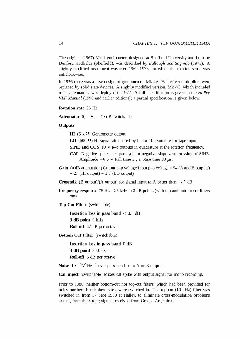
The original (1967) Mk-1 goniometer, designed at Sheffield University and built byDunford Hadfields (Sheffield), was described byBullough and Sagredo(1973). Aslightly modified instrument was used 1969–1976, for which the rotation sense wasanticlockwise.
In 1976 there was a new design of goniometer—Mk 4A. Hall effect multipliers werereplaced by solid state devices. A slightly modified version, Mk 4C, which includedinput attenuators, was deployed in 1977. A full specification is given in theHalleyVLF Manual (1996 and earlier editions); a partial specification is given below.
Rotation rate 25 Hz
Attenuator 0, ¡20, ¡40 dB switchable.
Outputs
HI (6 k ) Goniometer output.
LO (600) HI signal attenuated by factor 10. Suitable for tape input.
SINE and COS 10 V p–p outputs in quadrature at the rotation frequency.
CAL Negative spike once per cycle at negative slope zero crossing of SINE.Amplitude¡0:6 V Fall time 2¹s; Rise time 30¹s.
Gain (0 dB attenuation) Output p–p voltage/Input p–p voltage = 54 (A and B outputs)= 27 (HI output) = 2.7 (LO output)
Crosstalk (B output)/(A output) for signal input to A better than¡85 dB
Frequency response75 Hz – 25 kHz to 3 dB points (with top and bottom cut filtersout)
Top Cut Filter (switchable)
Insertion loss in pass band< 0:5 dB
3 dB point 9 kHz
Roll-off 42 dB per octave
Bottom Cut Filter (switchable)
Insertion loss in pass band0 dB
3 dB point 300 Hz
Roll-off 6 dB per octave
¡13 2 ¡1Noise 10 V Hz over pass band from A or B outputs.
Cal. inject (switchable) Mixes cal spike with output signal for mono recording.
Prior to 1980, neither bottom-cut nor top-cut filters, which had been provided fornoisy northern hemisphere sites, were switched in. The top-cut (10 kHz) filter wasswitched in from 17 Sept 1980 at Halley, to eliminate cross-modulation problemsarising from the strong signals received from Omega Argentina.
1.3. INSTRUMENT/SENSOR 15
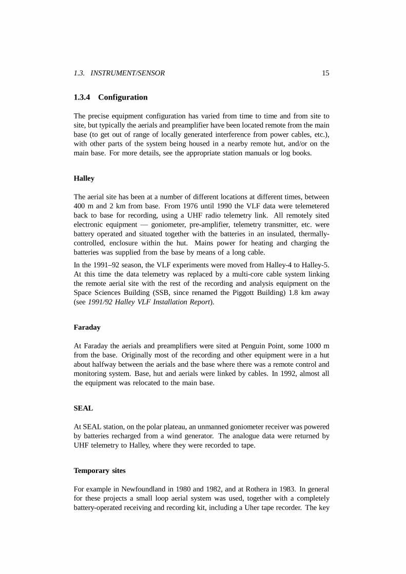
1.3.4 Configuration
The precise equipment configuration has varied from time to time and from site tosite, but typically the aerials and preamplifier have been located remote from the mainbase (to get out of range of locally generated interference from power cables, etc.),with other parts of the system being housed in a nearby remote hut, and/or on themain base. For more details, see the appropriate station manuals or log books.
Halley
The aerial site has been at a number of different locations at different times, between400 m and 2 km from base. From 1976 until 1990 the VLF data were telemeteredback to base for recording, using a UHF radio telemetry link. All remotely sitedelectronic equipment — goniometer, pre-amplifier, telemetry transmitter, etc. werebattery operated and situated together with the batteries in an insulated, thermally-controlled, enclosure within the hut. Mains power for heating and charging thebatteries was supplied from the base by means of a long cable.
In the 1991–92 season, the VLF experiments were moved from Halley-4 to Halley-5.At this time the data telemetry was replaced by a multi-core cable system linkingthe remote aerial site with the rest of the recording and analysis equipment on theSpace Sciences Building (SSB, since renamed the Piggott Building) 1.8 km away(see1991/92 Halley VLF Installation Report).
Faraday
At Faraday the aerials and preamplifiers were sited at Penguin Point, some 1000 mfrom the base. Originally most of the recording and other equipment were in a hutabout halfway between the aerials and the base where there was a remote control andmonitoring system. Base, hut and aerials were linked by cables. In 1992, almost allthe equipment was relocated to the main base.
SEAL
At SEAL station, on the polar plateau, an unmanned goniometer receiver was poweredby batteries recharged from a wind generator. The analogue data were returned byUHF telemetry to Halley, where they were recorded to tape.
Temporary sites
For example in Newfoundland in 1980 and 1982, and at Rothera in 1983. In generalfor these projects a small loop aerial system was used, together with a completelybattery-operated receiving and recording kit, including a Uher tape recorder. The key
16 CHAPTER 1. VLF GONIOMETER DATA
to this system is the Programmer Power Supply (PPS) described in theHalley VLFManual.
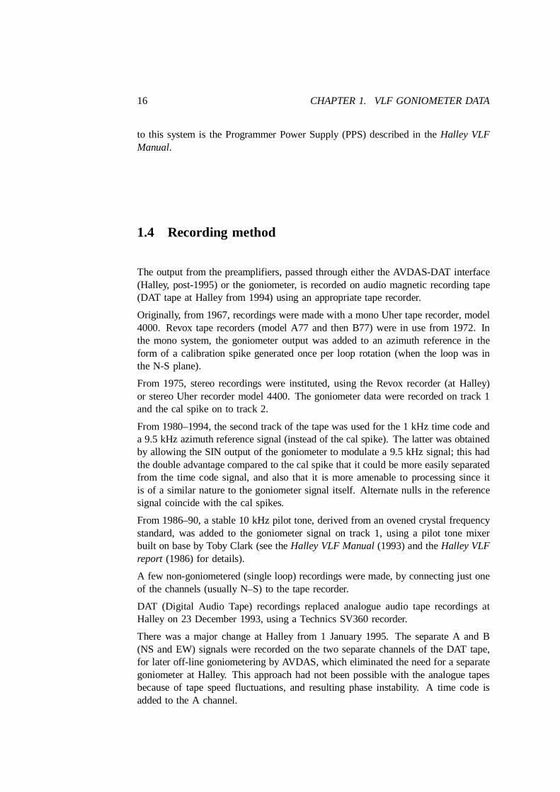
1.4 Recording method
The output from the preamplifiers, passed through either the AVDAS-DAT interface(Halley, post-1995) or the goniometer, is recorded on audio magnetic recording tape(DAT tape at Halley from 1994) using an appropriate tape recorder.
Originally, from 1967, recordings were made with a mono Uher tape recorder, model4000. Revox tape recorders (model A77 and then B77) were in use from 1972. Inthe mono system, the goniometer output was added to an azimuth reference in theform of a calibration spike generated once per loop rotation (when the loop was inthe N-S plane).
From 1975, stereo recordings were instituted, using the Revox recorder (at Halley)or stereo Uher recorder model 4400. The goniometer data were recorded on track 1and the cal spike on to track 2.
From 1980–1994, the second track of the tape was used for the 1 kHz time code anda 9.5 kHz azimuth reference signal (instead of the cal spike). The latter was obtainedby allowing the SIN output of the goniometer to modulate a 9.5 kHz signal; this hadthe double advantage compared to the cal spike that it could be more easily separatedfrom the time code signal, and also that it is more amenable to processing since itis of a similar nature to the goniometer signal itself. Alternate nulls in the referencesignal coincide with the cal spikes.
From 1986–90, a stable 10 kHz pilot tone, derived from an ovened crystal frequencystandard, was added to the goniometer signal on track 1, using a pilot tone mixerbuilt on base by Toby Clark (see theHalley VLF Manual(1993) and theHalley VLFreport (1986) for details).
A few non-goniometered (single loop) recordings were made, by connecting just oneof the channels (usually N–S) to the tape recorder.
DAT (Digital Audio Tape) recordings replaced analogue audio tape recordings atHalley on 23 December 1993, using a Technics SV360 recorder.
There was a major change at Halley from 1 January 1995. The separate A and B(NS and EW) signals were recorded on the two separate channels of the DAT tape,for later off-line goniometering by AVDAS, which eliminated the need for a separategoniometer at Halley. This approach had not been possible with the analogue tapesbecause of tape speed fluctuations, and resulting phase instability. A time code isadded to the A channel.
1.5. RECORDING SITES 17
1.5 Recording sites
² Halley.
² Faraday.
² Rothera.
² SEAL (Sheffield ELF/VLF Automatic Laboratory) — an unmanned, automaticVLF station operated on the ice plateau 120 km SSW of Halley (seeMatthewset al., 1979).
² Goniometer recordings made at “Depot 200”,»250 miles south of Halley (seeBAS report G3/1971/Z).
² Eastern Canada (conjugate to Halley): St. John’s, Cornerbrook, Dunmaglassand Fredericton (Southampton University; data at BAS), see (Strangeways etal., 1982); Newfoundland: St. Anthony, Deer Lake (see reports 1980, 1982).
² Ryvingen. Base of the Transglobe Expedition, where VLF recordings weremade for BAS by the expedition.
1.6 Dates/ times
1.6.1 Halley
1967–present (except 1968 and 1991)
1967 Sporadic»30 minute duration continuous recordings in support of Ariel-3.
1969–70Survey. Regular recording schedule, with times incrementing slowly. Record-ings every Wednesday in 1970.
1971–72Recordings in conjunction with Ariel-4, coincident recordings with Sanae,and passes of Isis satellite.
1973–89Recordings in conjunction with Siple transmitter.
1977–78 IMS related recordings. Special plasmapause campaigns and 24-hr longrecordings.
1979 Morning continuous recordings. Winter 24-hr recordings.
1980 Recordings in support of the SCATHA satellite, and the Siple sounding rocketprogramme.
1982 Recordings for DE-1 passes, and long CW Siple transmissions.
18 CHAPTER 1. VLF GONIOMETER DATA
1983 Recordings for DE-1 passes, and ISAAC.
1984 Recordings for AMPTE, and special AIS runs.
1985 Special AIS runs.
1986 Recordings for PROMIS (days 103–109, 118–119, 130–132, 142–145, 149–150, 155–157) and special Siple waveguide probing experiment.
1987 Recordings for WIPP (10–31 July) and summer Siple transmissions (from 5December).
1988 Recordings for QP campaign.
1990 Recordings for SAS/ACTIVE satellite.
1992 (Nov ’92 – Mar ’93) Special recordings for the ELBBO experiment.
Single loop recordings (mainly to study magnetospheric line radiation) were madeduring the following years (for more information, see the relevant reports and logbooks): 1979, 1983, 1984, 1986 (special 15 kHz recordings at 7.5 ips for the Siplewaveguide campaign).
1.6.2 Faraday
1985–1989; 1992–1995. Operations ceased on 21 December 1995. Faraday washanded to the Ukraine in February 1996, and renamedVernadsky.
1986 Recordings for PROMIS (see above) and special Siple waveguide probing ex-periment.
1987 No recordings except for the WIPP Campaign (10–31 July 1987)
1992 (Nov ’92 – Mar ’93) Special recordings for the ELBBO experiment
1994 Two weeks continuous recording in May in support of the University of Natalexpedition to Marion Island.
1.6.3 Rothera
March–April 1983; winter 1994.
1.6.4 Ryvingen
Winter 1980.
1.7. PHYSICAL MEDIA 19
1.6.5 SEAL
1977–78
1.6.6 Newfoundland
1972 (Southampton University); 1980; 1982.
1.7 Physical media
1/4 inch audio magnetic tape. A variety of makes of tape, tape speeds, spool sizes etc.have been used. Since the mid-1970s, Agfa type PEM369 tape has been used, mostlysupplied on 26.5 cm (10.5”) spools containing 1100 m (3600 ft) of tape, giving aplaying time of 192 min per side at 3.75 ips (9.5 cm/s). 13 cm (5”) diameter spoolshave also been used, giving a playing time of 56 min per side; these small spoolsmay be more convenient for calibrations, etc. All relevant details — time/date, tapenumber, sampling format, location, tape speed — are written on the tape leader andon the tape box.
At Halley, from 1994, DAT tapes were used. Type HBB DAT122 tapes have beensupplied; these run for 120 minutes.
1.7.1 Halley (until 1993)
Year(s) Tape speed (ips) Spool size (inch) Mono/ stereo1967–69 1.875* 5 mono1970–71 1.875 & 3.75 5 mono1972 1.875, 3.75 & (mainly) 7.5 5 & 10.5 mono1973–74 7.5 5 & 10.5 mono1975–76 7.5 5 & 10.5 stereo1977 3.75 (mainly) & 7.5 5 & 10.5 stereo1978–79 3.75 5 stereo1980 3.75 10.5 & 5 stereo1981 3.75 (mainly) & 7.5 5 & (mainly) 10.5 stereo1982 3.75 10.5 & 5 stereo1983–93 3.75 10.5 stereo
* Voice announcements at 15/16 ips.
1.7.2 Faraday
3Recordings have been made at a tape speed of3 ips (9.5 cm/s), on 10.5” tape spools.4
20 CHAPTER 1. VLF GONIOMETER DATA
1.8 Format description
For mono recordings, a single track was recorded on each side of the tape. For stereo(two-track) operation, recordings were made on each side of each tape (i.e. eachtrack occupies 1/4 of the width of the tape). The goniometer signal was recorded onChannel 1 (left) and the combined time code and azimuth reference on Channel 2(right). At Halley since 1995, the North-South signal (plus time code, frequencyshifted to 21.5 kHz) have been recorded on the left channel of the DAT tape, and theEast-West signal on the right channel, using a sampling rate of 48 kHz (per channel);this gives a flat frequency response to 22 kHz.
There are three different sampling formats:
1. Continuous recording
2. Synoptic recording: 1 minute in 5 (0–1, 5–6,. . . 55–56 minutes past the hour)
3. Synoptic recording: 1 minute in 15 (5–6,20–21, 35–36, 50–51 minutes pastthe hour)
Before 1977, only the continuous option was possible; 1977–84: continuous or 1-in-5;1985 onwards: all three. A decision on which option to use, a trade-off between tapecost and coverage, was made at the discretion on the local operator, with guidancefrom HQ. Since 1985, an attempt has been made to obtain complete coverage at aminimum of 1-in-15.
1.9 Size of data structures
The data unit is a tape. For 3600 ft long audio tapes, recorded at a tape speed of9.5 cm/s (3.75 ips), the nominal playing time for each side is 3.2 hours (192 minutes),i.e. 6.4 hrs per tape. For the three sampling programmes we therefore have:
Programme Hours/tape Days/tape Tapes/yrContinuous 6.4 .267 13691 in 5 32 1.33 2741 in 15 96 4 91
For DAT tapes, with a nominal playing time of 120 minutes per tape, we have:
Programme Hours/tape Days/tape Tapes/yrContinuous 2.0 .083 43801 in 5 10.0 .417 8761 in 15 30.0 1.25 292
Sometimes more than one recording, with a short gap interspersed, are recorded on the
1.10. VALIDATION 21
same tape. Sometimes there is a switch from one sampling programmes to another.This will be noted in the log, on the tape box, etc.
1.10 Validation
The best and really only convenient way of checking the data is to play the data tapeback through the AVDAS (see Section 1.15.1).
1.11 Anomalous or suspect data
For some recordings, the level has been set too high, so that the tape saturates forhigh level signals; some data can be lost or distorted, and spurious harmonics andcross-modulation products produced.
The receiver is very sensitive, and, being broad-band, some recordings especiallyearly ones suffer from interference, particularly 50 Hz harmonics from local sources.Wind noise has also occurred from time to time.
The time mark/ calibration tone has been missing on some tapes due to equipmentfaults. In 1989 at Halley, there was a problem with the tones “sticking” on. On sometapes the time code is too weak or distorted to be read reliably.
On some of the older tapes, there is a problem with oxide shedding. The tape headsrapidly get clogged up, lose high frequency response and need frequent cleaning.
1.12 Calibration
The calibration of the broadband system (goniometer and translated frequency), andalso of the VELOX (see Chapter 9), involves making data recordings with the nor-mally used arrangement, whilst inserting signals into the “front end” (aerials/preamplifier)of known intensity, frequency, and arrival azimuth.
Calibrations are done using three different methods (see Smith, 1995):
1. using a small rotatable 100 turn coil mounted near the centre of the loopaerials (At Halley from 1984 onwards, two orthogonal coils have been used toachieve rotation electronically by applying signals of the appropriate phase andamplitude.);
2. using a remote coil positioned 50 m from the aerial mast;
3. using a dummy aerial.
Details of calibration procedure have varied from time to time and from site to site,and the appropriate manuals and reports should be consulted for more details of these
22 CHAPTER 1. VLF GONIOMETER DATA
procedures. The theory of the calibration methods is given in theHalley VLF Manual.Normally calibration consists of both routine calibrations and full calibrations.
1.12.1 Routine calibration
Usually this is done with the small coil system, and the same injected signal alsoserves as a time marker. For more details, see Section 1.12.3. Since 1982 at Halleyand 1985 at Faraday, routine calibrations have been done automatically and consistof a tone once per minute: 1 s duration starting on the minute (3 s on 10 min,10 s on the hour). The tone consists of 5 frequencies: 488.28, 976.56, 1953.13,p
±3906.25, 7812.50 Hz; azimuth 045 (NE-SW); amplitude 1 pT rms (1= 5 pT rms¡3per frequency). [N.B. 1 pT́ 10 °.]
1.12.2 Full calibrations
These more extensive calibrations are carried out manually, and until 1996 wereusually done twice per year, once before and once after the winter season’s recordings;since 1997 the calibrations have been done annually. Usually they involve more thanone of the calibration methods enumerated above, and generally include azimuthchecks, frequency response and sensitivity checks. The times of the calibrations arenoted in the log book, and also documented by completing calibration forms whichare returned to Cambridge for filing. Usually a separate tape is used for calibrations,and is identified by a leadingC, e.g. CZ93A. Recently the calibrations have beenworked up in Lotus 1-2-3 spreadsheets; information may be found on the UASDserver ato:“uasd“wave“cals“ .
1.12.3 Time Marks on Halley VLF Tapes
1. (Before Feb 1971) A time mark was made by connecting the output of anaudio signal generator (Advance HIE) 1000 Hz 22 V rms to the long intercomcables running from base to the goniometer hut. This was picked up by thegoniometer, detectable but not calibrated in any way. A burst of the abovesignal was applied for 5 seconds ending exactly on a minute, the time beingannounced on the tape and noted in the log book.
2. (Feb 1971 – 24 Feb 1972) The above system was continued. For runs donemanually from the hut, a five second gap was inserted instead of a time mark.
3. (24 Feb 1972 – 2 Mar 1972) Cal mark made by feeding a signal to the 100-turncalibration coil set in the centre of loops in the North-South plane. The signalwas 0.25 V rms 1 kHz from a Venner oscillator.
4. (2 Mar 1972 – beginning of 1975) Time marks (again 5 s ending on a minute);signal equivalent to a 1 pT rms sine wave propagating North-South. The
1.12. CALIBRATION 23
calibration signal was supplied either from a Venner oscillator in the hut (10 Vrms 1 kHz sine) or from base with an Advance signal generator (6 V rms 1 kHzsine).
5. (19 Jul 1972 – 11 Dec 1972) Automatic calibration marker working exceptfor intermittent breaks. Signal supplied to calibration coil from oscillator onbase along long lines. Duration: on hour — 10 s, 30 minutes — 5 s, 10,20, 40, 50 minutes — 1 s. Pulse starts 2 s after closure of clock contacts.Clock error noted in the log book. Signal used is 1 kHz non-sinusoidal to giveharmonic frequencies. Intensity to give 0.51 V rms across cal. coil and 2 k
series resister. During breakdown of automatic system, system 4) was revertedto; comparisons of systems 4) and 5) on the same tape can be found on 446G.
6. (11 Dec 1972 – 7 Jun 1973) As 5) but modified to be more sinusoidal. Intensity0.23 V rms across 2 k resistor and cal. coil. Again 4) was used when theautomatic system broke down.
7. (From the beginning of 1975) A new automatic calibration oscillator was in-stalled. It ran off the (crystal) observatory clock. 7 kHz 1 pT to the calibrationcoil (N–S); 1 s starting on the minute (3 s on the 10-minute, 10 s on the hour).
8. (From the beginning of 1980) The observatory clock was replaced by a pro-grammer unit driven from the time code generator.
9. (From February 1981) a new 5-frequency calibration generator was installed.±Same times as above. Calibration coil at 045 (NE–SW). Frequencies 488.28,
976.56, 1953.13, 3906.25, 7812.50 Hz. Amplitude 1 pT rms per componentp(total 5 pT rms).
10. (From 22 January 1982) The same as above but the amplitudes were reducedpto 1 pT rms total (1= 5 pT rms per component). A similar system was usedat Faraday.
1.12.4 Time code
A Datum 9300 time code generator was installed at Halley in 1980; it ran from arubidium standard and provided a continuous IRIG-B time code (1 kHz carrier). Thiswas recorded on track 2 of the tape after the azimuth reference at 9.5 kHz had beenadded. A similar system was operated at Faraday, but using a Rapco 300 time codegenerator and an ovened crystal oscillator. At Halley since early 1997 the time codegenerator has been slaved to the IRIG-B output of the IRIS GPS receiver. The latteralso outputs an estimate of the timing accuracy, which is logged by the IRIS system;it appears rarely to exceed 100¹s, and is usually much less.
24 CHAPTER 1. VLF GONIOMETER DATA
1.13 Naming/numbering conventions
In general, each tape is given a unique number. For analogue tapes, side 1 andside 2 of the tape are indicated by a suffix G or R (for green leader and red leader,respectively); this is not appropriate for DAT tapes.
1.13.1 Halley
1967 tapes were unnumbered, but identified by date (labelled and voice recording ontape).
From 1969 onwards, tapes were given a serial number starting with 1 (13 March1969), which did not reset each year. This had reached 3157 by 4 January 1991when this system was discontinued. For a few cases in 1971–72, 13 cm and 26 cmspool tapes had duplicated numbers.
Since 1992 tapes have been numberedZyy-nnn whereyy is the year (e.g. 93) andnnn is a chronological serial number running from 001, and resettingeach year.
Single loop recordings were labelledUGnnand special tapes for the Siple waveguideprobing experiment (1986)WGyynn. for 1986.
Calibration tapes were labelledCnn.
1.13.2 Faraday
In 1985–86, Faraday followed the same system as Halley, with numbers increasingfrom 1, and not resetting each year. From 1988 onwards, they were labelledyynnnwith Faraday indicated in words.
From 1992–95 tapes were numberedFyy-nnn whereyy was the year (e.g. 93) andnnn was a chronological serial number running from 001, and resetting each year.
1.13.3 SEAL
Tapes were labelledPnn (P for plateau).
1.14 Catalogues
1.14.1 Log books
All recordings are entered in the log book with relevant comments, e.g.
² start and stop times/dates

1.14. CATALOGUES 25
² tape number
² sampling format (continuous, synoptic 1/5 or synoptic 1/15)
² time checks
² clock corrections
² recording level changes
² changes in other settings e.g. tape speed or attenuator setting
² notes on VLF activity
² any equipment problems and action taken
² any calibrations done
Paper log books are kept in duplicate, with the top copy returned to Cambridge andthe carbon copy retained on the base.
Besides the hand written paper log book, machine-readable versions have also beenproduced, since 1984 at Halley and 1988 at Faraday, in a standard format (seeSection 1.14.2). These are ASCII text files which are available on the server ato:“uasd“wave“data“catlogs“broadlog“ ; they are also saved on MS-DOSformat discs (in the disc box marked ‘VLF log files’). They are created directly us-ing a text editor, or more easily by running a programmeMKLOG(for details, see theHalley VLF Manual). A FORTRAN programmeLOGCAT(originally written for aVAX, but now available as a DOS EXE programme) scans a machine-readable logfile and produces a catalogue of broadband recordings in the standard format (seebelow).
The machine-readable log should contain not only all the information required toform the catalogue of recordings that is held in Cambridge, but also details of anyaction, change to the system, human error or equipment breakdown which might haveaffected the data recorded and would therefore be required at a later date to interpretthe recorded data.
Year-long log files are namedssyy.LOG wheress is the two-letter code for thereceiver sites (HB for Halley, FA for Faraday, etc.) andyy is the 2-digit year,e.g. HB92.LOG. These files are concatenated from monthly files sent back fromAntarctica namedssyymmm.LOG, wheremmmis the month, e.g.HB92JUL.LOG.
1.14.2 Log file format specification
Each line of the log file is formed of four fields; these will be known here as the DAY,TIME, ACTION and COMMENTS fields. They are 5, 8, 8, and 106 characters widerespectively, and may contain characters as specified below. N.B. The ‘ ’ characterin the text that follows represents a blank character (except in the strings ending_AZ.
26 CHAPTER 1. VLF GONIOMETER DATA
DAY Field
The DAY field consists of columns 1 to 5 and is formed thus:
_ddd_
whereddd represents the day of the year. The DAY field may be blank, and the lineis then interpreted either as part of an extension line (see below) or as an action thatoccurs on the same day as the previous action (i.e. you may miss out the day on thesecond and subsequent entries made during a certain day).
TIME Field
The TIME field is columns 6 to 13 and contains the UT time in hours and minutes.Where seconds are specified, these are separated from the minutes by a decimal pointor a colon thus:
1203.20
or
2330:00
The TIME field may be blank when the action referred to does not need an exacttime to be specified (e.g. it is not important exactly when a tape is put on the recorder— only the actual start time of the recording needs to be known precisely). The fieldmay also be blank if the action specified occurs at the same time as the previousaction (i.e. you may miss out the time on the second and subsequent entries made atthat time).
ACTION field
The ACTION field of eight characters (columns 14 to 21) describes the reason thatthe entry was made. It may be blank. If it is blank, and the two preceding fields arealso blank, then the line is simply an extension line of the previous line and so noday, time or action is associated with it.
If it is not blank, then the characters allowed in the field must be one of the stringsspecified here. These may broadly classified into two sets, those that give informationconcerning the type of programme being recorded (known here asProgrammestrings)and those that do not (known here asNormal strings).
Allowed ProgrammeStrings:
1 IN 5 (Note the upper caseIN ) 1 in 5 recording programme has started at thistime.
1.14. CATALOGUES 27
1 IN 15 1 in 15 recording programme has started at this time.
CONT Continuous recording programme has started at this time.
OFF Recording (of whatever programme) ceased at this time. This string maynot be the first programme string after anotherOFFprogramme string, and maynot be the first programme string after aTAPEnormal string.
Allowed normal strings:
TAPE A new tape has been mounted on the tape recorder, but no recording hasstarted (the start of a recording should be indicated instead by one of the firstthree programme strings described above). The last programme string musthave beenOFFThe first eight characters of the COMMENTS field on this lineare taken as the tape number. The sixth character in the COMMENTS field istaken to be the ”leader” character that appears in the catalogue.
CLOCK The error of the time-code generator relative to UT was calculated at thistime. The first six characters of the COMMENTS field are read as a realnumber and represent the time error in seconds (a positive number means thatthe clock was fast relative to UT, and a negative one that it was slow.) NOOTHER INFORMATION SHOULD BE RECORDED IN THE COMMENTSFIELD ON A CLOCKLINE.
REF AZ or CAL AZ Follow with calibration tone bearings in the COMMENTSfield, e.g. 45.6, 37.2, 46.8, 42.8, 47.3.
ARG AZ Follow with Omega Argentina bearing in the COMMENTS field, e.g.138.2.
SYNC The clock synchronised with the correct UT time.
WPM Indicates that the first three comment characters contain the number ofwhistlers counted in one minute at the time given (must be¸ 1).
COMMENTS field
The columns 22 to 127 are the 106-character comments field containing either com-ments upon activity at the time or reasons why a particular action was necessary. Forcertain actions, the comments field will contain data such as the number and leadercode of a tape, or the clock error, as specified above.
1.14.3 Example of log entries
M indicates left margin.
28 CHAPTER 1. VLF GONIOMETER DATA
¡file B89APR.LOG¿M FARADAY BROADBAND LOG. APRIL 1989.M (Continuing tape 89024 Red.)M 102 0405:00 WPM 0 WHISTLERSM 1005 WPM 0M 1040 OFFM TAPE 89035GM 1040 1 IN 15M 1605 WPM 0 WHISTLERSM 2205 WPM 0M 103 0405 WPM 7M 1005 WPM 0 WHISTLERS. HISS, CHORUS.M 1605 WPM 0M 2205 WPM 0M 2250 CLOCK -0.1M 104 0405 WPM 12 WHISTLERS, FAINT.M 1005 WPM 15 WHISTLERS, FAINT.M 1021 OFFM TAPE 89035RM 1021 1 IN 15M 1605 WPM 0 WHISTLERSM 2205 WPM 0
1.14.4 Catalogue format
Information on each recording is held in a catalogue file in the format describedbelow.
1.14. CATALOGUES 29
COLUMNS CHARACTERS DATA1. . . 2 2 YEAR (last two figures of)4. . . 6 3 MONTH (first three letters of)8. . . 9 2 DAY OF MONTH
11. . . 13 3 DAY OF YEAR15. . . 18 4 START TIMEHHMMin UT. 9999 if unknown20. . . 23 4 STOP TIMEHHMMin UT. 9999 if unknown
(recordings are split at 0000)25. . . 26 2 STATION in standard two letter abbreviations
28 1 PROGRAMMES = 1 IN 5 (synoptic),C =continuous;F = 1 IN 15 (synoptic)
30. . . 34 5 TAPE IDENTIFICATION36. . . 37 2 REEL SIZE to nearest cm
39 1 LEADER or TRACK IDENTIFICATION41. . . 44 4 TAPE SPEED in inches per second46. . . 50 5 CLOCK ERROR in seconds with respect to UT
Negative figures mean times on tape are slow wrt UT.9999 if unknown
52 1 Y if whistlers reported, otherwise-54. . . 56 3 Maximum no. of whistlers reported,999 if no record
Columns 36–44 are not relevant for DAT tapes.
1.14.5 Standard abbreviations for bases
BR BermudaCW Cape Wrath, ScotlandD1 Dynamics Explorer 1 satelliteDL Deer Lake, NewfoundlandFA Faraday, AntarcticaHB Halley, AntarcticaMR Marsh, AntarcticaPA Palmer, AntarcticaPU Punta Arenas, ChileRA Rothera, AntarcticaRO Roberval, QuebecRY Ryvingen, AntarcticaSA St. Anthony, NewfoundlandSI Siple, AntarcticaSL Seal, AntarcticaSP South Pole, Antarctica
All catalogues files are available on the server ato:“uasd“wave“data“catlogs“broadcat“ ;they are also saved on MS-DOS floppy discs in the box marked ‘VLF Catalogue files’.They have names constructed of: 2-letter abbreviation (as above), last 2 figures of
30 CHAPTER 1. VLF GONIOMETER DATA
year of data,.CAT . For example:HB83.CAT. An example of part of a cataloguefile is shown below:
86 JUL 8 189 0945 1605 HB S 2303 26 G 3.75 -0.55 Y 286 JUL 8 189 1605 2400 HB F 2303 26 G 3.75 -0.58 _ 99986 JUL 9 190 0000 0130 HB F 2303 26 G 3.75 -0.62 _ 99986 JUL 9 190 0130 0601 HB S 2303 26 G 3.75 -0.63 _ 99986 JUL 9 190 0605 1940 HB S 2303 26 R 3.75 -0.65 Y 386 JUL 9 190 1940 2007 HB C 2303 26 R 3.75 0.31 _ 99986 JUL 9 190 2013 2026 HB C 2304 26 G 3.75 0.31 _ 99986 JUL 9 190 2026 2400 HB S 2304 26 G 3.75 0.31 Y 2086 JUL 10 191 0000 1105 HB S 2304 26 G 3.75 0.31 Y 2086 JUL 10 191 1225 2400 HB S 2304 26 G 3.75 0.31 Y 586 JUL 11 192 0000 0340 HB S 2304 26 G 3.75 0.31 Y 5
A folder of printed catalogues exists in the data room.
1.14.6 Catalogue handling programmes available
These were written in FORTRAN by P. Jenkins, in 1984 for the DEC PDP-11. Theywould probably run on a VAX but have not yet been converted to run on a PC. Formore information see theUK Analysis manual.
CATSRTSorts a standard format file into chronological order by start time.
CATPLT Produces a plot of the data coverage.
CATSIM Produces a file of times when recordings were being made simultaneouslyat two stations, by comparing the times of recordings in the two standard formatfiles. Since its output is in standard format,CATSIMcan be used for comparingoutput with a third station’s catalogue to produce a set of times of simultaneousrecordings at 3 (or more) stations, and so on.
CATNIP Places zeros in blanks in the start and stop times of a file. This is to avoidtimes such as “0703” being confusingly written as “ 7 3” when a processingprogram uses two integers for HH and MM.
1.15 Analysis methods
1.15.1 AVDAS
The best way of analysing the data is to use the AVDAS, either the one at Halley orthe one at Cambridge. With this powerful spectral analysis system, the data may beexamined in great detail in ways which were not possible or easy before.
1.15. ANALYSIS METHODS 31
At Cambridge, tapes are analysed using the Analogue VLF Data Facility, currentlysituated in Room 214. Its centrepiece is the AVDAS, but it also contains Revox B77reel-to-reel and Panasonic SV- 3700 playback decks, amplifiers, filters, frequencytranslator, frequency standard, time code readers, time code demultiplexer, audioamplifier, loud-speaker and headphones.
AVDAS (Mk-2) was engineered and manufactured by High Greave Associates, Sheffield,and is fully described in their manual (see also Smithet al., 1994). It is a devel-opment of the Mk-1 system, circa 1982. The original unit was supplied in 1990but various improvements have been made since then. The system consists of thefollowing components:
1. The HGA DSP-II Digital Processing System hardware.
2. Firmware for the DSP-II.
3. A PC host. Software resides on the host to control the operation of the DSP-IIand to log files containing the results of any analysis to hard disc.
For data analysis, AVDAS is hooked up to a tape recorder to play back the data tape,and to an audio amplifier for aural monitoring.
To use the system, switch on the AVDAS, and if necessary change the baud-rate to9600 (instructions in Section 1.16.1). TheAVDASprogramme is run on the host PC,using the following command line:
AVDAS [/TL=n] [/FL=m] [/TF=¡filename¿]
/TL selects the device for controlling the tape recorder for playback; at Cambridge itis set to 0 for the special parallel interface./FL selects the device for communicatingwith the DSP-II; at Cambridge it is set to 1 for the COM1 serial port. The defaultcommand line is in the“AVDAS“ directory on the PC, calledAV.BAT. For moreinformation, see theAVDAS Manual.
The following facilities are among those available:
1. Control the playback tape recorder.
2. View the data in a variety of formats: spectrograph with a range of time andfrequency resolutions and averaging; A-scan (frequency versus amplitude); timeseries plot; etc.
3. Save and load spectrogram files.
4. Make measurements from the screen with a mouse and cursor, and optionallystore the results in a file.
5. Scale whistlers.
6. Measure bearings.
32 CHAPTER 1. VLF GONIOMETER DATA
7. Capture interesting events and print out the data on the Paintjet colour printer(see examples in Figs. 1.1 and 1.2).
8. Run the “Quick look facility” to produce summary spectrographic plots (seeexample in Fig. 1.3).
Some of the AVDAS commands available at theAVDAS¿prompt are as follows (seetheAVDAS Manualfor a full set and complete documentation):
AVPOWERIntegrated power in a specified frequency band or time interval.
AZIMUTH Arrival azimuth for goniometer data.
COMMENTPut comment in results file.
CORRTIMECorrect timing errors.
HARDCOPYProduce graphics file for plotting.
HELP List available commands.
LOAD Load spectrogram from disc.
PALETTE Specify colour or monochrome palette.
POINTS Log frequency-time points.
RESULTSWrite results to file.
SAVE Save spectrogram to disc.
SCALE Scale whistlers, using 3-point, 2-point or 1-point scaling.
SET Set spectrum analyser settings: transform size, frequency range, redundancy,averaging, gain, maximum and minimum amplitude, tape recorder (0 = DAT;1 = Revox), etc.
SET MODE TIMEEnable saving of time series data.
SET MODE VECTOREnable azimuth processing using vector, i.e. two-channel (DAT)data.
SHOWShow current settings.
STATION Specify recording site.
SYSTEMExecute DOS command.
TAKE Execute batch file of AVDAS commands.
YEAR Specify recording year.
1.16. ANALYSIS SOFTWARE 33
1.15.2 Other procedures
Methods for doing the following are described in theUK Analysis Manual:
1. Spectrographic (35-mm) film making (this is probably no longer feasible, ornecessary).
2. Tape copying.
3. Making synoptic (1-in-5) recordings from continuous recordings.
4. Use of the ‘spheric eliminator’.
5. Making Trimpi measurements from analogue tape recordings.
1.16 Analysis software
AVDASprovides most of what is required.
CALPROCprocesses tapes containing calibration signals, producing calibration fileswhich can be used for correcting the azimuth measurements.
SPECATproduces a catalogue of spectrum files on the disc.
QLOOKproduces “Quick look” summary plots.
TAPESF For measuring the intensity of spherics recorded on the tape. Written byKeith Yearby. For more information, see separate documentation.
MLRSCANFor studying magnetospheric line radiation (MLR). Written by KeithYearby. For more information, see separate documentation.
1.16.1 VLF quick look system — QLOOK
Introduction
The quick look system (QLOOK) has been designed by High Greave Associates(Sheffield) for producing spectrographic summary plots from analogue tape-recordedVLF radio wave data. Here is reproduced an abbreviated version of the manufac-turer’s documentation, which is to be found in theAVDAS documentationfolder. Thesystem is primarily intended to work from tapes recorded with a time code, but willalso support tapes without time code.
The output from the system is in the form of graphics files. These may be plottedon a colour or monochrome printer supporting a resolution of at least 180 dots perinch assuming a suitable driver programme is available. Drivers are available which
34 CHAPTER 1. VLF GONIOMETER DATA
support colour or monochrome plots on the HP PaintJet printer or a PostScript printer,and for previewing on the PC screen (see Appendix E).
The system supports plots in continuous, 1in5 and 1in15 formats. Format conversion,that is producing a plot in a different format from that in which the tape was recorded,is supported for tapes recorded with time code. In continuous mode there is one hourper page, in 1in5 mode six hours per page, and in 1in15 mode 12 hours per page.One output file is produced for each page of data; the maximum size of the file isabout 300 k-bytes.
The standard frequency range of the plot is 8 kHz. Other available ranges are 4, 16and 32 kHz. Each spectrum contains 40 points which gives a resolution of 200 Hzon the standard range. The time resolution is 72 spectra per minute independent ofthe frequency range.
The system consists of two modules. One (QLOOK.S28) is downloaded into theHGA DSP-II and operates it to produce averaged spectra at the rate required. Thesespectra are transmitted to the PC where the second module (QLOOK.EXE) formatsthe data into graphics files.
Command set
Commands are entered at theQLOOK¿prompt. It is necessary to enter only enoughcharacters to match the name uniquely. This applies also to parameters of theSETcommand.
DEBUG nControls the display of debugging information.n = 0 (default) meansno debugging information,n = 1 displays a message for each packet of datareceived from the DSP-II.
LOAD Downloads the DSP-II software module (QLOOK.S28).
QUIT LeavesQLOOKand returns to DOS.
REMOTEPasses the rest of the command line to the DSP-II. Available remote com-mands are:
REMOTE SET GAINgain where gain is a number between 0 and 4, corre-sponding to full scale input voltages between 10 and 0.1 volts peak. Thedefault is 2 (1V).
REMOTE SET FREQfreq wherefreq may be one of 5k, 10k, 20k, or 40k. Thedefault is 10k (Hz) although only the lower 80% of the range is displayedon the plot.
REMOTE SET AVTYPEtype wheretypemay beLOGor POWER. Logarithmicaveraging (the default) suppresses impulsive signals such as spherics, buton the time scale of these plots it also tends to suppress whistlers. Thismay not be desirable so the alternative of power averaging is provided.
1.16. ANALYSIS SOFTWARE 35
REMOTE SHOWdisplays the values of the above parameters.
SET parameter valueThe settable parameters and corresponding range of values areshown in the table below.
DAY integer 1..366MAXAMP integer 1..96MINAMP integer 0..MAXAMP-1MODE OFF CONT 1IN5 1IN15STATION any text string up to 8 charactersSYNC OFF ONTIME hour minute second as separate numbersYEAR integer
Most of these are self explanatory but a few notes are given here.MAXAMPandMINAMPcontrol the amplitude range (in dB) of the data on the plot. Valuesoutside this range are clamped. The value of theDAY, STATION andYEARparameters are used only in the title on each page of the plot.
The SYNCparameter controls whether theQLOOKinternal clock (DAY andTIME) parameters are automatically synchronised to the time code on the tapes.There is no point in trying to set the values ofDAYor TIME if SYNCis ONbecause they will be overwritten when the next spectrum with a valid time isreceived from the DSP-II.
SHOWDisplays the value of the settable parameters.
STATUS Displays the debug level.
Starting up
The PC should be connected to the DSP-II host computer port using the standardcable. The fileQLOOK.EXEshould be in the default directory or in the path. Thefile QLOOK.S28must be in the default directory. If the fileQLOOK.INI exists inthe default directory the programme will read initialisation commands from there.
The system should be started using the following procedure.
1. On the PC start theQLOOKprogram with the command:QLOOK [port]whereport is 1 (default) or 2 depending on which COM port is used for theconnection to the DSP-II.
2. Switch on the DSP-II; if it directly enters an application then exit this (forDSP-FFT click mouse right button).
3. Enter the SYSTEM menu.
4. Change the BAUDRATE to 9600.
36 CHAPTER 1. VLF GONIOMETER DATA
5. Enter the LOAD menu.
6. On the PC type the commandLOADat theQLOOK¿prompt. Several rows ofdots should be printed on the PC screen.
7. When the load has completed, on the DSP-II exit the SYSTEM menu.
8. A QLOOK button should now have appeared on the DSP-II top level menu;click the mouse on this to start QLOOK on the DSP-II. The DSP-II screen willgo blank, while on the PC the top line on the screen should show details ofthe data packets now being received. No further use is made of the screen ormouse of the DSP-II.
The system should now be ready for use.
Operating
First ensure the system has been started as described in the previous section.
Play a trial section of the tape and check the details of the data on the top lineof the screen. If a synchronised plot is to be produced the time display must bealmost error free. The system will cope with bursts of errors lasting a maximum of8 seconds. Theov (overload) indicator should be zero most of the time; if not usetheREM SET GAINcommand to reduce the gain. Note the minimum and maximumamplitudes. Typical values may be around 30 and 70; if they are a lot lower, considerincreasing the gain but only if this does not cause overloads.
Rewind the tape to the beginning.
Use theSET MIN andSET MAXcommands to set the amplitude range for the plot.Suitable values will probably be similar to those noted above; experience will tell.
For a synchronised plot, setSYNCto ON, set theMODEas required (i.e.CONT, 1IN5or 1IN15 ) and then start the tape. When the tape has finished, any follow-on tapemay be started directly. For a synchronised plot, it is not necessary to set theMODEto OFFwhile changing tapes. To produce a plot in a different format from the tape(e.g. a1IN5 plot from a continuous tape) it is simply necessary to set theMODEtothe type of plot required. It is not necessary to inform the system that the tape is ina different format.
For a non-synchronised plot, setSYNCto OFF, set theDAYandTIME to the start timeof the tape and carefully position the tape at the start of the data. Then simultaneouslyset theMODEas required and start the tape. As soon as possible after the tape hasfinished set theMODEto OFF. Repeat the procedure above to run any follow-on tapes.The system does not support format conversion in non-synchronised mode.
When the set of tapes has been completed, use theQUIT command to leaveQLOOKand return to DOS.
1.17. DERIVED DATA SETS 37
The file corresponding to each page of the plot has a name of the formQndddhh.GRFwheren is 1 for CONT, 2 for 1IN5 and 3 for1IN15 , anddddhh are the day andhour of the start of the page.
The files may be previewed on the screen or plotted on a PostScript or PaintJet printer(see Appendix E).
If more tapes are to be run,QLOOKmay be re-started by typing theQLOOKcommandat the DOS prompt. It should not be necessary to reload the DSP-II provided thishas not be powered down or reset.
1.17 Derived data sets
² Processed calibration files (output ofCALPROC); seeAVDAS Manual.
² Analysis results files (output of AVDASRESULTScommand); see Section 1.17.1.
² Spectrogram files (output of AVDASSAVEcommand).
² Hardcopy plots (output of AVDASHARDCOPYcommand); for examples, seeFigs. 1.1 and 1.2.
² 35 mm film spectrogram rolls; see Section 1.17.2
² “Quicklook plots”; for example, see Fig. 1.3.
1.17.1 Results files
The results of scaling whistlers on the AVDAS have been saved in results files ofthe formRddda-yy.TXT whereddd is the day number,yy is the year, anda is adistinguishing letter (if necessary).
1.17.2 Film spectrograms strips
A library of 35 mm film strips has been created and is stored in the data room(Room 230); a film winder is also there for viewing them. The strips provide a goodsummary of what is on the data tapes. The “Quick look” facility (Section 1.16.1)which runs on the AVDAS, provides a summary of tape contents and replaces thefunction of the film spectrograms, which are, however, still valuable for the olderdata.
The following information is written at the beginning of each section of film:
² Catalogue No.
² Tape No.
38 CHAPTER 1. VLF GONIOMETER DATA
² Date
² Filming speed
² Frequency range
Catalogue No. indicates the station at which the data were recorded, the year and theindividual identification number for that piece of film (e.g.HB82-059 ). Tape No.indicates original tape number and side (e.g.1763R). The individual films strips arejoined together and wound on numbered spools for compact storage.
Times are labelled showing the start, finish and hour points on the film.
For most of the survey film strips, a frequency range of 0–10 kHz and a filmingspeed of 0.016”/sec (1” per minute) have been used.
A record card was filed for each catalogue number, in the format below:
__________________________________: :
Catalogue No. : HB82-059 3/7/82 : DateTape No. : 1763R 1925-2125 : Start/Finish
Month, Day : July 3 (1 in 5) : Programme: :
Frequency range : 0-10 kHz :Filming speed : 0.016”/sec :
: :Spool No. : HB82-009 :
__________________________________
The cards are in card catalogue boxes in the data room, filed in station groups andthen in chronological order.
1.17.3 Quicklook plots
For some stations and years, the tape data have been systematically played backthrough the quicklook system, and bound folders of plots have been produced. Theseare handy sets of summary plots for flicking through and picking out promising eventsof particular kinds.
1.18 Archiving
It is not practical to archive in digital form the vast amount of analogue data held onthe original tapes. Many of the early data tapes are stored in BAS central archives,
1.19. DOCUMENTATION 39
in an environmentally controlled area. Ideally they should be respooled periodically,to guard against “print-through”, though in practice there are no resources to do this.
1.19 Documentation
² AVDAS Manual, High Greave Associates, Sheffield, January 1993.
² VLF Preamplifier Model 2 Manual, High Greave Associates, Sheffield, 1993.
² Installation of the VLF Experiments at Halley-5, 1991–92, A.J. Smith, BASReference ZV/1991/I3.
² UK Analysis Manual, A.J. Smith (ed.), August 1989.
² Halley VLF Manual, A.J. Smith and J. Digby (eds.), June 1995.
² VLF Plateau Station Manual, October 1976.
² VLF Field Programme, Halley Bay October 1971, A.J. Smith, BAS ReferenceG3/1971/Z.
1.20 References
1.20.1 Unpublished
Report on a visit to Newfoundland, June–July 1980A.J. Smith, September 1980.
Halley VLF report 1983, K.H. Yearby, BAS Reference Z/1983/I4.
Halley VLF report 1984, K.H. Yearby, BAS Reference Z/1984/I4.
Halley VLF report 1985, T.D.G. Clark, BAS Reference Z/1985/I3.
Halley VLF report 1986, T.D.G. Clark, BAS Reference Z/1986/I2.
Report on a trip to Halley, 1994/95 Season, A.J. Smith, March 1995.
Faraday VLF report 1985, M.A. Clilverd, BAS Reference F/1985/01.
1.20.2 Published
² Bullough K., Hughes A.R.W., Hudson T., Hickinson D., Broomhead P. andTomlinson P. (1968) The Sheffield University experiment on the satellite Ariel3. J. Sci. Inst. Series 2,1, 77–85.
40 CHAPTER 1. VLF GONIOMETER DATA
² Bullough K. and Sagredo J.L. (1973) VLF goniometer observations at HalleyBay, Antarctica — I. The equipment and the measurement of signal bearing.Planet. Space Sci.21, 899–912.
² Jenkins P.J. (1984) Magnetospheric Research: ELF/VLF whistler programme,in Report of Scientific Work of the Transglobe Expedition 1979–1982, ed.R. Fiennes, pp. 13–29.
² Matthews J.P., Smith A.J. and Smith I.D. (1979) A remote unmanned ELF/VLFgoniometer receiver in Antarctica. Planet. Space Sci.27, 1391–1401.
² Smith A.J. (1995) VELOX: a new VLF/ELF receiver in Antarctica for theGlobal Geospace Science mission. J. Atmos. Terr. Phys.57, 507–524.
² Smith A.J., Hughes P. and Yearby K.H. (1994) DSP-II and its applications: aunified approach to the acquisition and analysis of VLF radio wave data forresearch. The Radio Scientist5(3), 120–123.
² Strangeways H.J., Rycroft M.J. and Jarvis M.J. (1982) Multistation VLF direction-finding measurements in Eastern Canada. J. Atmos. Terr. Phys.44, 509–522.

Chapter 2
Translated frequency data
2.1 Brief description
Frequency translated broadband tape recordings.
2.2 Detailed description
At Halley frequency-translated recordings were made of the 15–25 kHz, for studyingVLF transmissions which occur in this band. The band is shifted downwards by15 kHz to 0–10 kHz so that it can be recorded better on analogue audio magnetictape. A similar system operated at Faraday but the frequency range 15–25 kHz wastranslated to 2–12 kHz to avoid aliasing problems with the Omega signals whichwere stronger at Faraday.
The translated frequency recordings were used for analysing the occurrence, phaseand amplitude of Trimpi events on any VLF transmissions occurring in the receivedband, in particular those which were not received by the OMSK receiver (which couldreceive only four signals at once: 2£MSK and 2£ Omega, see Chapter 8). A phasereference (pilot) tone was added to the tape (at Halley but not at Faraday). Its purposewas to serve as a phase reference, so that phase as well as amplitude fluctuationson recorded transmitter signals (e.g. Trimpi events) could be measured by correctingfor tape speed variations (‘wow’ and ‘flutter’). Because of skew between channels,the reference had to be recorded on the same channel as the data. A time code wasrecorded on a separate tape track, as for the goniometer recordings. At Halley, forconvenience, this was the same combined time code and azimuth reference signal asused on the standard goniometer recordings, although for non-goniometered signalsthe azimuth reference is not relevant.
41
42 CHAPTER 2. TRANSLATED FREQUENCY DATA
2.3 Instrument/sensor
2.3.1 Halley
Beginning in 1984, the broadband signal was passed through a goniometer to thePrinceton TRA-50 frequency translator. A continuous stable phase reference (equiv-
±alent to a 1 pT 20 kHz 45 azimuth signal) was added via the small calibrationcoil.
From 1992, the input to the frequency translator was non-goniometered (from the N–S loop) and the pilot tone was 10 kHz added after translation (equivalent to 25 kHz),rather than 20 kHz added at the aerials. The equipment was set up as follows: thechannel A VLF signal was applied to the input of the TRA-50 frequency translator(actually in 1992 the goniometered signal was used by mistake; this was corrected in1993). The settings were: 1 V, F = 15000 Hz, B = 10 kHz, XLATE ON. The outputof the TRA-50 went to the pilot tone mixer (‘GONIO IN’). The pilot tone mixeroutput (‘SIG+10 kHz’) went to the tape recorder input. One of the 1 MHz outputsof the rubidium frequency standard connected to the pilot tone mixer 1 MHz input.This set-up could also be used for non-translated, non-goniometered recordings bysetting the translator to ‘XLATE OFF’. For details on the pilot tone mixer, see theHalley VLF Manual(1993) and theHalley VLF report(1986).
2.3.2 Faraday
A frequency translator manufactured by High Greave Associates was used. Signalswere from the A channel (N–S loop).
2.4 Recording method
2.4.1 Halley
The translated signal with pilot tone was recorded to track 1 of a second Revoxtape recorder (the first being used for the standard goniometer recordings). Mixedtime-code and azimuth reference tone were recorded on track 2 as for goniometerrecordings. Control of the tape recorder was as for the goniometer recordings.
2.4.2 Faraday
The translated signal was recorded to track 1 of a second Revox tape recorder (thefirst being used for the standard goniometer recordings). Time code was recorded ontrack 2. Control of the tape recorder was as for the goniometer recordings.
2.5. RECORDING SITES 43
2.5 Recording sites
Halley, Faraday.
2.6 Dates/ times
2.6.1 Halley
1984–90; 1992–94.
1987 recordings for the WIPP campaign: 19–31 July, 0300–0315 UT and 0815–0830 UT, and also 20 September to 4 October, 18–10 UT.
1988–90 for Trimpi campaign following magnetic storms (0300–0920 UT).
1992 for tethered satellite experiment (August).
2.6.2 Faraday
1989; 1992–94,
1989 Recordings throughout the year, concurrently with 0–10 kHz goniometer record-ings, at 1-in-5 and 1-in-15 schedules.
1992 About one tape per month, on a continuous sampling schedule, at times of highVLF activity.
2.7 Physical media
The same analogue audio magnetic tapes were used as for the goniometer recordings(see Chapter 1).
2.8 Format description
Similar to the goniometer recordings (see Chapter 1) except for the frequency trans-lation. Continuous, 1-in-5, and 1-in-15 sampling schedules were available.
2.9 Size of data structures
Same comments as for the goniometer recordings (see Chapter 1).
44 CHAPTER 2. TRANSLATED FREQUENCY DATA
2.10 Validation
Same as for the goniometer recordings (see Chapter 1), i.e. use the AVDAS.
2.11 Anomalous or suspect data
For tapesTX8616R – TX8624G NS and EW loops were accidentally interposed(extra calibrations were done for this unintentional set-up).
2.12 Calibration
Calibrations for the frequency translated recordings were generally done at the sametime as the main goniometer and VELOX calibrations, since they used the sameset-up. Usually the small calibration coil was used to simulate signals of knownintensity, azimuth and frequency in the translated band (typically 15–25 kHz). Theprecise frequencies used were chosen on the day, to fit in gaps in the spectrum wherethere were no or only weak transmissions. For more details, consult the relevantmanuals and reports. Calibrations were documented on the calibration form.
2.13 Naming/numbering conventions
In 1984, tapes were labelledTPnn. In 1985 they were labelledTXnn; in 1986TXyynn .
At Faraday in 1989, tapes were labelledyyTnn , e.g.89T01 .
Since 1992 tapes have been numberedsyyT-nnn wheres is the station code (Zfor Halley, F for Faraday, etc.),yy is the year (e.g. 93) andnnn is a chronologicalserial number running from 001 (reset each year).
2.14 Catalogues
Prior to 1992, catalogues were less well organised than for the goniometer recordings,and in general it will be necessary to refer to the original log books.
From 1992, catalogues and machine readable log files were produced in the sameway and in the same format as for goniometer recordings (see Chapter 1), but had adistinguishing letterT, e.g. HB92T.LOG, HB92T.CAT.
2.15. ANALYSIS METHODS 45
2.15 Analysis methods
As for the goniometer recordings (see Chapter 1), i.e. use the AVDAS (see examplein Fig. 2.1). There is a frequency offset option (SET OFFSET ¡freq¿ from theAVDAS¿prompt), so that translated frequencies can be scaled correctly.
2.16 Analysis software
AVDAS software (see Section 1.15.1).
2.17 Derived data sets
None.
2.18 Archiving
As for goniometer data.
2.19 Documentation
² Halley VLF report 1986, T.D.G. Clark, BAS Reference Z/1986/I2.
² Faraday VLF report 1989/90, J.S. Robertson, BAS Reference F/1989/IV1.
² Halley VLF Manual, A.J. Smith, January 1993.
² Frequency Translator Manual, High Greave Associates, Sheffield, 1988.
2.20 References
² Clark T.D.G. and Smith A.J. (1990) Quasi-periodic particle precipitation andassociated Trimpi activity at Halley, Antarctica. J. Atmos. Terr. Phys.52,365–375.

46 CHAPTER 2. TRANSLATED FREQUENCY DATA
Part C
Digital data
47

Chapter 3
AVDAS logger data
3.1 Brief description
ELF/VLF wave intensity at four frequencies.
3.2 Detailed description
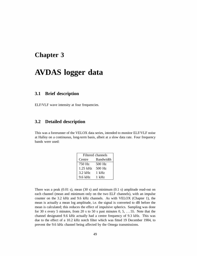
This was a forerunner of the VELOX data series, intended to monitor ELF/VLF noiseat Halley on a continuous, long-term basis, albeit at a slow data rate. Four frequencybands were used:
Filtered channelsCentre Bandwidth750 Hz 500 Hz1.25 kHz 500 Hz3.2 kHz 1 kHz9.6 kHz 1 kHz
There was a peak (0.01 s), mean (30 s) and minimum (0.1 s) amplitude read-out oneach channel (mean and minimum only on the two ELF channels), with an impulsecounter on the 3.2 kHz and 9.6 kHz channels. As with VELOX (Chapter 1), themean is actually a mean log amplitude, i.e. the signal is converted to dB before themean is calculated; this reduces the effect of impulsive spherics. Sampling was donefor 30 s every 5 minutes, from 20 s to 50 s past minutes 0, 5, . . . 55. Note that thechannel designated 9.6 kHz actually had a centre frequency of 9.3 kHz. This wasdue to the effect of a 10.2 kHz notch filter which was fitted 19 December 1984, toprevent the 9.6 kHz channel being affected by the Omega transmissions.
49
50 CHAPTER 3. AVDAS LOGGER DATA
3.3 Instrument/sensor
The data were taken using the multi-channel receiver (MCR). This instrument, de-signed at Sheffield University, was based on the ELF/VLF receiver flown on theAriel-4 satellite and consisted essentially of a number of hard-wired band-pass filters(see preceding section for the characteristics) and a means for sampling them. Thereceiver was originally used at Halley in 1971–74 to coincide with Ariel-4. At thattime data were recorded only on paper chart and are not accessible digitally, althoughthe charts still exist (see Introduction).
The receiver was modified by removing the integral preamplifier and multiplexer, andsimplifying the resetting arrangements and the power supply. It was then redeployedfor use with the AVDAS Mk1 in 1983.
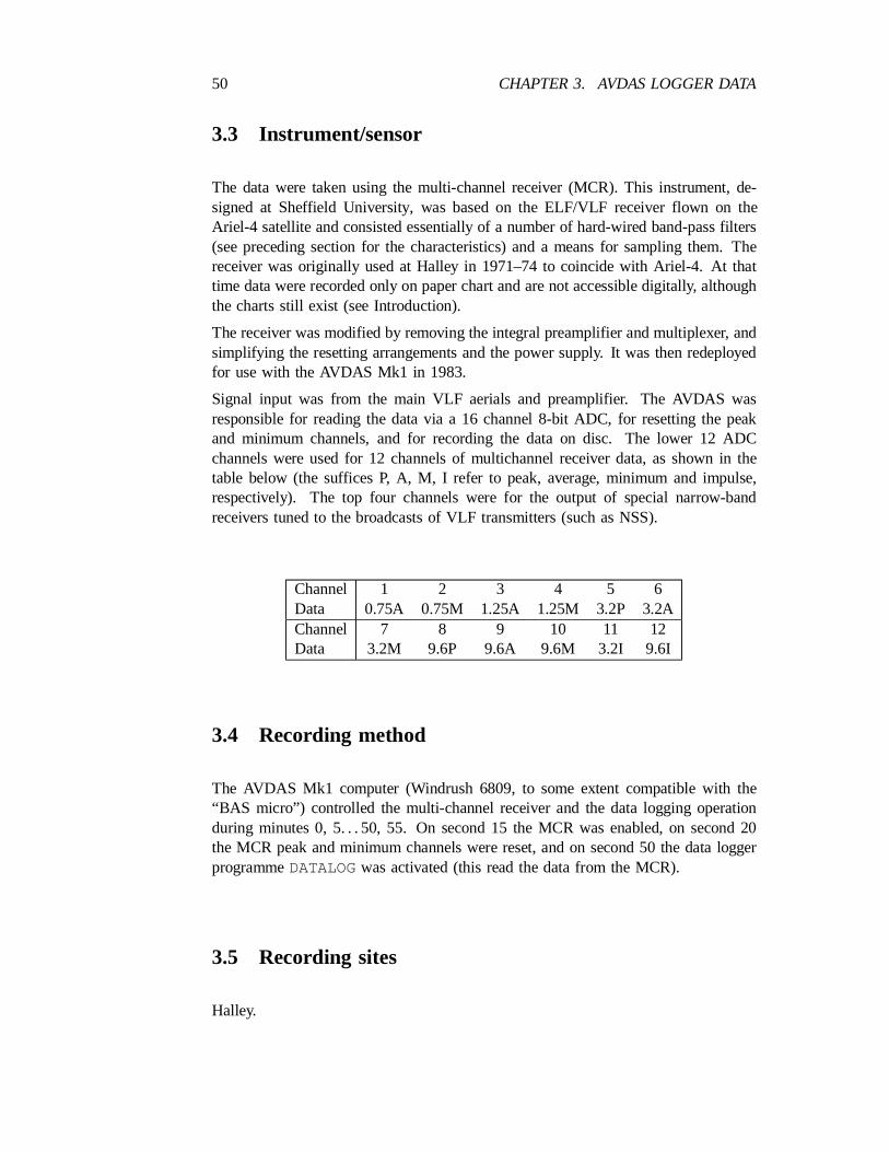
Signal input was from the main VLF aerials and preamplifier. The AVDAS wasresponsible for reading the data via a 16 channel 8-bit ADC, for resetting the peakand minimum channels, and for recording the data on disc. The lower 12 ADCchannels were used for 12 channels of multichannel receiver data, as shown in thetable below (the suffices P, A, M, I refer to peak, average, minimum and impulse,respectively). The top four channels were for the output of special narrow-bandreceivers tuned to the broadcasts of VLF transmitters (such as NSS).
Channel 1 2 3 4 5 6Data 0.75A 0.75M 1.25A 1.25M 3.2P 3.2AChannel 7 8 9 10 11 12Data 3.2M 9.6P 9.6A 9.6M 3.2I 9.6I
3.4 Recording method
The AVDAS Mk1 computer (Windrush 6809, to some extent compatible with the“BAS micro”) controlled the multi-channel receiver and the data logging operationduring minutes 0, 5. . . 50, 55. On second 15 the MCR was enabled, on second 20the MCR peak and minimum channels were reset, and on second 50 the data loggerprogrammeDATALOGwas activated (this read the data from the MCR).
3.5 Recording sites
Halley.
3.6. DATES/ TIMES 51
3.6 Dates/ times
Nominally 24-hrs/day from 1983 to 1990, though there are a few data gaps.
3.7 Physical media
8” floppy discs, formatted under the FLEX operating system; since transferred toCD-ROM.
3.8 Format description
A data record (corresponding to one hour) consists of 12 sub-records (one for eachsample taken every 5 minutes) of 21 bytes in length. Bytes 0 to 15 contain thedigitised signals on the 16 analogue inputs to the ADC. Bytes 16 to 19 contain thetime of that sub-record (100 days, tens and units days, tens and units hours, tens andunits minutes). Byte 20 contains the current VLF recording mode (0 = OFF, 1 = 1-IN-5, 2 = 1-IN-15 and 3 = CONT) at that time. Each hour’s data was accumulatedin memory and written to a previously created random-access disc file after the lastsample for the hour had been collected (at 55 mins past the hour). The files werenormally created long enough to hold 15 days of data, though they usually containonly around 14 days of valid data, a new file being created once per fortnight. Thefirst FLEX sector (252 bytes) of the file is a logger information record. Only the first4 bytes are used. The first two contain an integer offset which when subtracted fromthe hour of year gives the data record in the file corresponding to that hour. The hourof year number is defined to be ‘(day number)£ 24 + (UT hour)’. The second twobytes are the integer number of data records in the file.
The digital values in the file,V , may be converted to amplitudeA expressed as dB¡33 2 ¡1wrt 10 T Hz by the equation
A = A + a(V ¡ V )0 0
whereA is the value of A corresponding to a 1 pT rms signal in the centre of the0
band. This is 63 dB for the 500 Hz wide ELF channels (0.75 kHz and 1.25 kHz),and 60 dB for the 1 kHz wide VLF channels (3.2 kHz and 9.6 kHz).V is the0
corresponding value ofV , i.e. the value ofV for a 1 pT signal.
3.9 Size of data structures
The 1-hr data records are12 £ 21 = 252 bytes long. With the 252-bytes headerrecord, a 15-day files is(15£ 24 + 1)£ 252 = 90972 bytes long.
52 CHAPTER 3. AVDAS LOGGER DATA
3.10 Validation
The MS-DOS programmeCHECKLGmay be used for listing and checking the loggerdata files; for details, see Section 3.16.3.
3.11 Anomalous or suspect data
In 1983–84, the 9.6 kHz peak channel was contaminated by the 10.2 kHz Omegatransmission.
There were no 0.75 kHz data after 11 August 1990, when that channel failed.
A list of shorter intervals containing invalid data is contained in the fileAVDAS.NUL(see Section 3.17.1).
3.12 Calibration
3.12.1 Quick calibration
A quick calibration was done near the beginning of each logger file. This was doneby switching on the standard 5-frequency calibration tone (see Section 1.12.3) for thewhole of a one-minute sampling period (time recorded in the log book).
3.12.2 Full calibrations
The main multi-channel receiver calibrations were generally done twice per year.Dates and times were noted in the log book and a calibration form completed. Formore details, see theAVDAS manual, 1989. Note that the nominal 9.6 kHz channelwas calibrated using 9.3 kHz signals, because of the 10.2 kHz notch filter.
Amplitude scale
Calibration coil Signal 1 pT equivalent; frequencies of 0.75, 1.25, 3.2 and 9.3 kHz;maintained for two sampling periods each.
Dummy aerial Signals of 1 pT, 0.1 pT and 0.01 pT at 0.75, 1.25, 3.2 and 9.3 kHzfor one receiver sampling period each. Then no input signal (noise level).
Frequency response
To determine the frequency response of each channel, the dummy aerial was used tosimulate signals of the following frequencies with an equivalent amplitude of 1 pT.
3.13. NAMING/NUMBERING CONVENTIONS 53
0.75 and 1.25 kHz channels0.25, 0.5, 0.75, 1.0, 1.25, 1.5 and 1.75 kHz.
3.2 kHz channel 2.2, 2.7, 3.2, 3.7, 4.2 kHz.
9.6 kHz channel 8.6, 9.0, 9.3, 9.6, 10.0 kHz.
These are the centre frequencies of each channel, a half bandwidth away from thecentre and a full bandwidth away from the centre. The output should be about 3 dBdown at a half bandwidth away, and about 20 dB down at a full bandwidth awayfrom the centre frequency.
Impulse counter
For details, see theAVDAS manual, 1989.
3.13 Naming/numbering conventions
Logger files have been given names of the formLGddd-yy.DAT whereddd is theday number of the start of the file andyy is the year. For some files in 1990, thehyphen was omitted. Files from 1986–88, which were processed on a PDP-11, wererenamedLdddyy.AVD to make the filenames acceptable to the RT-11 operatingsystem.
3.14 Catalogues
Because of the low data rate, there are relatively few files and extensive machine-readable catalogue files are not essential. Catalogues exist in printed form, andoriginal ‘Flex’ style catalogues for each year, of the formDIR-yyyy.txt , areincluded on the archive CD-ROM discs along with the corresponding data files.Catalogues may be produced using the programmeCATLOG(see below).
3.15 Analysis methods
Analysis is done on a PC using the MS-DOS software described below. At presentthe data are accessed from a local CD-ROM drive.
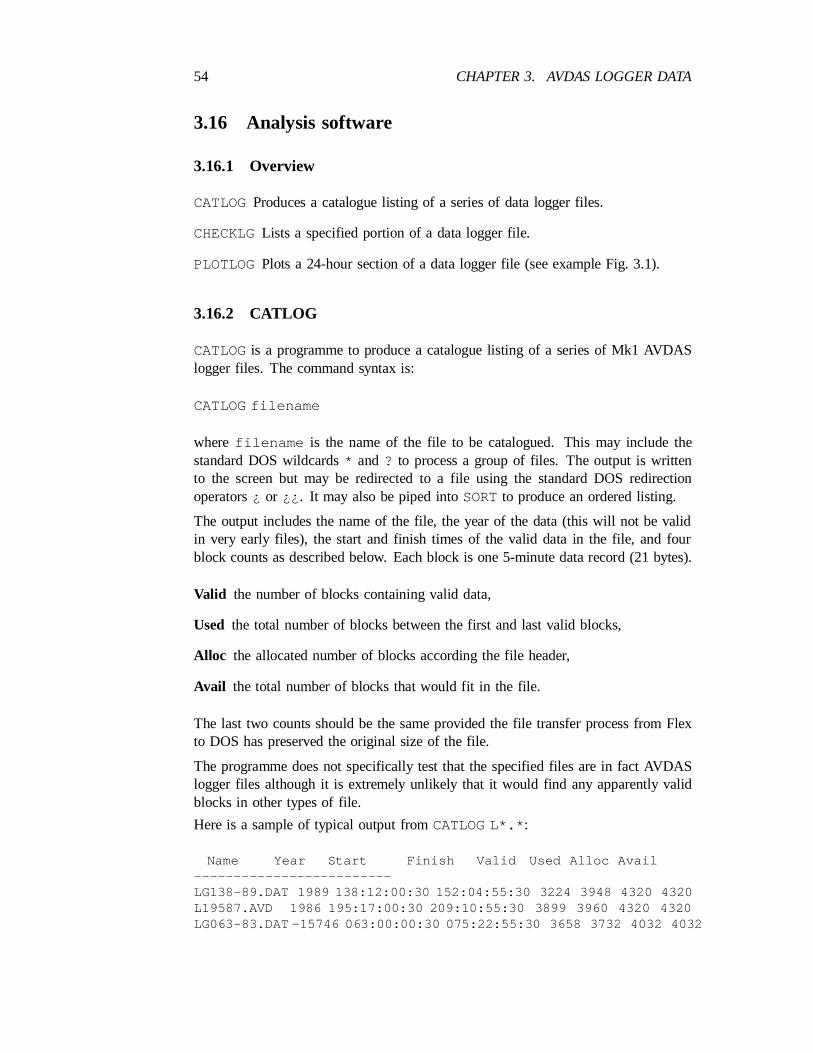
54 CHAPTER 3. AVDAS LOGGER DATA
3.16 Analysis software
3.16.1 Overview
CATLOGProduces a catalogue listing of a series of data logger files.
CHECKLGLists a specified portion of a data logger file.
PLOTLOGPlots a 24-hour section of a data logger file (see example Fig. 3.1).
3.16.2 CATLOG
CATLOGis a programme to produce a catalogue listing of a series of Mk1 AVDASlogger files. The command syntax is:
CATLOG filename
where filename is the name of the file to be catalogued. This may include thestandard DOS wildcards* and? to process a group of files. The output is writtento the screen but may be redirected to a file using the standard DOS redirectionoperators¿ or ¿¿. It may also be piped intoSORTto produce an ordered listing.
The output includes the name of the file, the year of the data (this will not be validin very early files), the start and finish times of the valid data in the file, and fourblock counts as described below. Each block is one 5-minute data record (21 bytes).
Valid the number of blocks containing valid data,
Used the total number of blocks between the first and last valid blocks,
Alloc the allocated number of blocks according the file header,
Avail the total number of blocks that would fit in the file.
The last two counts should be the same provided the file transfer process from Flexto DOS has preserved the original size of the file.
The programme does not specifically test that the specified files are in fact AVDASlogger files although it is extremely unlikely that it would find any apparently validblocks in other types of file.
Here is a sample of typical output fromCATLOG L*.* :
Name Year Start Finish Valid Used Alloc Avail—————————————————————————LG138-89.DAT 1989 138:12:00:30 152:04:55:30 3224 3948 4320 4320L19587.AVD 1986 195:17:00:30 209:10:55:30 3899 3960 4320 4320LG063-83.DAT -15746 063:00:00:30 075:22:55:30 3658 3732 4032 4032
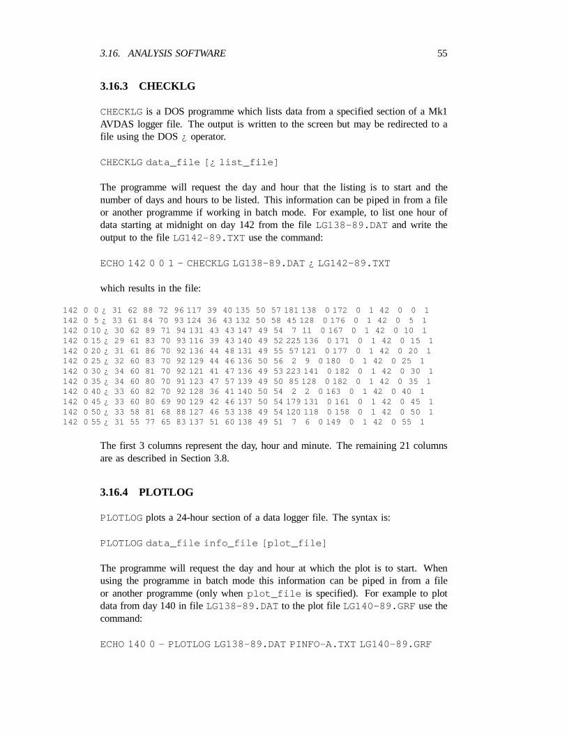
3.16. ANALYSIS SOFTWARE 55
3.16.3 CHECKLG
CHECKLGis a DOS programme which lists data from a specified section of a Mk1AVDAS logger file. The output is written to the screen but may be redirected to afile using the DOS¿ operator.
CHECKLG data_file [¿ list_file]
The programme will request the day and hour that the listing is to start and thenumber of days and hours to be listed. This information can be piped in from a fileor another programme if working in batch mode. For example, to list one hour ofdata starting at midnight on day 142 from the fileLG138-89.DAT and write theoutput to the fileLG142-89.TXT use the command:
ECHO 142 0 0 1 — CHECKLG LG138-89.DAT ¿ LG142-89.TXT
which results in the file:
142 0 0 ¿ 31 62 88 72 96 117 39 40 135 50 57 181 138 0 172 0 1 42 0 0 1142 0 5 ¿ 33 61 84 70 93 124 36 43 132 50 58 45 128 0 176 0 1 42 0 5 1142 0 10 ¿ 30 62 89 71 94 131 43 43 147 49 54 7 11 0 167 0 1 42 0 10 1142 0 15 ¿ 29 61 83 70 93 116 39 43 140 49 52 225 136 0 171 0 1 42 0 15 1142 0 20 ¿ 31 61 86 70 92 136 44 48 131 49 55 57 121 0 177 0 1 42 0 20 1142 0 25 ¿ 32 60 83 70 92 129 44 46 136 50 56 2 9 0 180 0 1 42 0 25 1142 0 30 ¿ 34 60 81 70 92 121 41 47 136 49 53 223 141 0 182 0 1 42 0 30 1142 0 35 ¿ 34 60 80 70 91 123 47 57 139 49 50 85 128 0 182 0 1 42 0 35 1142 0 40 ¿ 33 60 82 70 92 128 36 41 140 50 54 2 2 0 163 0 1 42 0 40 1142 0 45 ¿ 33 60 80 69 90 129 42 46 137 50 54 179 131 0 161 0 1 42 0 45 1142 0 50 ¿ 33 58 81 68 88 127 46 53 138 49 54 120 118 0 158 0 1 42 0 50 1142 0 55 ¿ 31 55 77 65 83 137 51 60 138 49 51 7 6 0 149 0 1 42 0 55 1
The first 3 columns represent the day, hour and minute. The remaining 21 columnsare as described in Section 3.8.
3.16.4 PLOTLOG
PLOTLOGplots a 24-hour section of a data logger file. The syntax is:
PLOTLOG data_file info_file [plot_file]
The programme will request the day and hour at which the plot is to start. Whenusing the programme in batch mode this information can be piped in from a fileor another programme (only whenplot_file is specified). For example to plotdata from day 140 in fileLG138-89.DAT to the plot fileLG140-89.GRF use thecommand:
ECHO 140 0 — PLOTLOG LG138-89.DAT PINFO-A.TXT LG140-89.GRF
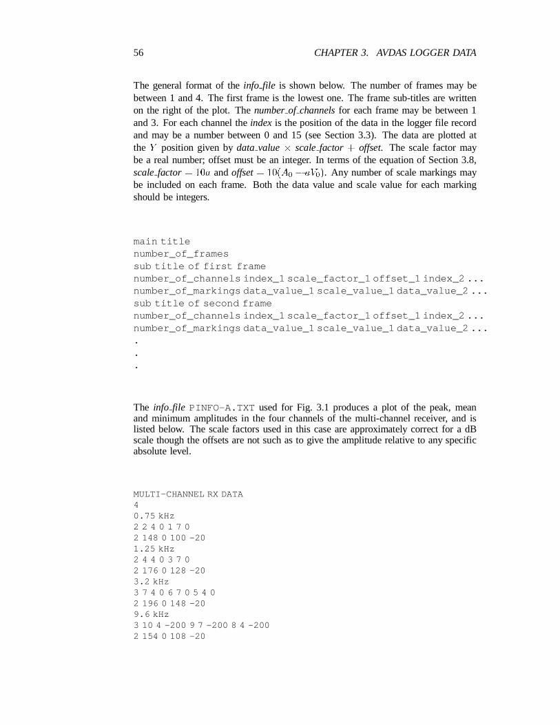
56 CHAPTER 3. AVDAS LOGGER DATA
The general format of theinfo file is shown below. The number of frames may bebetween 1 and 4. The first frame is the lowest one. The frame sub-titles are writtenon the right of the plot. Thenumber of channelsfor each frame may be between 1and 3. For each channel theindex is the position of the data in the logger file recordand may be a number between 0 and 15 (see Section 3.3). The data are plotted atthe Y position given bydata value£ scale factor+ offset. The scale factor maybe a real number; offset must be an integer. In terms of the equation of Section 3.8,scale factor= 10a andoffset= 10(A ¡ aV ). Any number of scale markings may0 0
be included on each frame. Both the data value and scale value for each markingshould be integers.
main titlenumber_of_framessub title of first framenumber_of_channels index_1 scale_factor_1 offset_1 index_2 ...number_of_markings data_value_1 scale_value_1 data_value_2 ...sub title of second framenumber_of_channels index_1 scale_factor_1 offset_1 index_2 ...number_of_markings data_value_1 scale_value_1 data_value_2 ......
The info file PINFO-A.TXT used for Fig. 3.1 produces a plot of the peak, meanand minimum amplitudes in the four channels of the multi-channel receiver, and islisted below. The scale factors used in this case are approximately correct for a dBscale though the offsets are not such as to give the amplitude relative to any specificabsolute level.
MULTI-CHANNEL RX DATA40.75 kHz2 2 4 0 1 7 02 148 0 100 -201.25 kHz2 4 4 0 3 7 02 176 0 128 -203.2 kHz3 7 4 0 6 7 0 5 4 02 196 0 148 -209.6 kHz3 10 4 -200 9 7 -200 8 4 -2002 154 0 108 -20
3.17. DERIVED DATA SETS 57
3.17 Derived data sets
3.17.1 auxiliary files
AVDAS.CAL
This ‘ascii’ file contains the calibration information necessary for converting the rawvalues in the data to absolute intensities, via the equation of Section 3.8. Each linecontains 23 numbers. The first three are integers representing the year (two-digit),day of year and hour at which the calibrations are valid. The following ten pairs ofnumbers represent thea andV values, determined from calibrations, for each of the0
channels 1–10 (see Section 3.3). Calibration constants at times between those listedin the file may be found by interpolation.
AVDAS.NUL
This ‘ascii’ file contains a list of invalid data intervals (in chronological order). Eachline contains four integers. The first three represent the year (two-digit), day of yearand hour of the start of the invalid data, whilst the fourth is the hour (on the sameday) at which the good data resume. Invalid data intervals spanning midnight aresplit into two or more consecutive lines.
3.17.2 Statistical and other plots
A number of IDL programmes have been written for the Smith and Jenkins (1998)paper.RDLOGGER.PROreads the data values out of the file, and usesAVDAS.CALAVDAS.NUL, to calibrate them and reject invalid ones. The data may be displayedin a variety of formats, including plots of medians, day plots (DAYPLOT.PRO) andUT vs. day of year plots (YEARPLOT.PRO). The programmes may be found in thedirectory o:“uasd“wave“logger“ . Further discussion is beyond the scope ofthis manual.
3.18 Archiving
All the data have been archived on to a single CD-ROM (with backup), namedVLF-LOGGER-0_1200_A.
3.19 Documentation
² AVDAS Mk1 manual, K.H. Yearby, 1989.
58 CHAPTER 3. AVDAS LOGGER DATA
² Multi-channel receiver manual, University of Sheffield, 24 November 1970(with added note of modifications made to interface with AVDAS, 1982).
3.20 References
² Bullough K., Hughes A.R.W., Hudson T., Hickinson D., Broomhead P. andTomlinson P. (1968) The Sheffield University experiment on the satellite Ariel3. J. Sci. Inst. Series 2,1, 77–85.
² Jenkins P.J. (1988) A survey of ELF/VLF noise at Halley, Antarctica, andassociated studies. Ph.D. thesis, University of Sheffield.
² Smith A.J. and Yearby K.H. (1987) AVDAS — A microprocessor-based VLFsignal processing and spectral analysis facility for Antarctica. Br. Antarct. Surv.Bull. No. 75, 1–15.
² Smith A.J. and Jenkins P.J. (1998) A survey of natural electromagnetic noisein the frequency rangef = 1–10 kHz at Halley station, Antarctica: 1. Radioatmospherics from lightning. J. Atmos. Solar-terr. Phys. (in press).
Chapter 4
Trimpi data
4.1 Brief description
Narrow band digital measurements of VLF transmitter signals.
4.2 Detailed description
The amplitude and/or phase and/or bearing of selected VLF transmitters (e.g. Siple,NAA, NSS, GBR) have been measured at Halley and recorded digitally to disc.This has mostly been done with the aim of looking for trimpi events, before theOPAL/OMSK receivers dedicated to this task were deployed. A variety of fixed andtunable narrow-band receivers have been used.
4.2.1 1983 Trimpi and Ureka measurements
Relative amplitude and phase of Siple transmissions were measured during specialSiple transmission campaigns. Supporting chart records of NAA amplitude and bear-ing were also made during the campaign periods. Similar measurements of Siple am-plitude and phase, using similar methods, were made during the Siple earth-ionospherewaveguide probing experiment in 1986.
4.2.2 ISAAC measurements
Special recordings of NAA and GBR amplitude and azimuth in 1983 were made insupport of the International South Atlantic Anomaly Campaign.
59
60 CHAPTER 4. TRIMPI DATA
4.2.3 Trimpi measurements
From 1984 onwards, amplitude and sometimes bearing of a selected transmitter wererecorded.
4.2.4 Logger measurements
21.4 kHz (NSS) and 16 kHz (GBR) were recorded to channels of the AVDAS datalogger.
4.2.5 Omega measurements
Amplitudes of signals from all eight Omega transmitters received on 13.6 kHz wererecorded digitally in 1986, in support of the Halley meteorology programme whichused an Omega-based system for its radio-sondes.
4.3 Instrument/sensor
The basic wideband signal from the standard VLF aerial and preamplifier has beenprocessed in a variety of ways to produce the final analogue signals which have beendigitally recorded. For more information, see the relevant report.
4.3.1 1983 Trimpi and Ureka measurements
The B loop (E-W) signal was taken via the TRA-50 frequency translator, set totranslate the signal to 5 Hz, to the DSP interface (see chapter on the time seriesdata).
4.3.2 ISAAC measurements
Small loops aerials located near the caboose containing the main equipment wereused (narrow-band measurements above 10 kHz were less affected by interference).The signals were fed from a goniometer to a fixed tuned receiver (tuned to GBRand NAA) and thence to a special ISAAC interface (seeHalley VLF Report, 1983).Amplitude and azimuth were 10 s averaged.
4.3.3 Trimpi measurements
Goniometer signals (no top-cut filter) were taken through a tunable VLF receiver(built to replace the fixed GBR/NAA one) to the ISAAC interface. Output was to
4.4. RECORDING METHOD 61
the AVDAS, channels 14 (amplitude) and 15 (azimuth) for digitisation. SeeHalleyVLF report (1985).
4.3.4 Logger measurements
The tunable receiver and the 16 kHz fixed tuned receiver were used.
4.3.5 Omega measurements
13.6 kHz signals received on the E-W loop, were translated down to 25 Hz using theTRA-50 frequency translator, and input to channel 15 of the AVDAS.
4.4 Recording method
For more information, see the relevant report.
4.4.1 1983 Trimpi and Ureka measurements
The AVDAS Mk-1 programmeSAMPLERwas used to digitise the input signal at10 Hz and write the data to a disc file.
Chart records of records of NAA amplitude and phase at 30 cm/hr were made usingthe ISAAC interface (see below).
4.4.2 ISAAC measurements
The analogue data were taken to channels 14 and 15 of the AVDAS general purposeinterface, digitised and logged to the data logger files, along with data from themulti-channel receiver (see the chapter on the AVDAS logger data). A changeoverrelay multiplexed NAA and GBR alternately, on even and odd multiples of 5 minutesrespectively.
4.4.3 Trimpi measurements
The sampling, digitising, and recording was done using the AVDAS Mk-1 programmeWASPROG, seeHalley VLF report(1985).
62 CHAPTER 4. TRIMPI DATA
4.4.4 Logger measurements
21.4 kHz amplitude (47 s time constant) was recorded on logger channel 0 and 16 kHzon channel 13.
4.4.5 Omega measurements
The AVDAS Mk-1 programmeOMSAMPLE, a version ofSAMPLER, was used todigitise the input signal and write the data to a disc file.
4.5 Recording sites
Halley.
4.6 Dates/ times
1983 ISAAC 23 June – 23 August; UREKA 18–26 July; TRIMPI 15 September0635-0655 UT; NAA chart records: 1 September – 1 October.
1984 Trimpi data: 11 August – 30 September.
1985 Trimpi data: August – September.
1986 Trimpi data: for the days of the PROMIS campaign (see Chapter 1) and specialtrimpi campaign 28 August – 23 September; Siple amplitude/phase for the Siplewaveguide experiment: 23–28 June and 21–25 July at 0800–0845 UT and 15–19 September and 22–26 September at 1700–1745 UT. Omega: ten 24-hourperiods once per month from day 90.
1988–90Trimpi data: 5 nights following magnetic storms.
4.7 Physical media
FLEX format floppy discs (mostly 8-inch).
4.8 Format description
4.8.1 1983 Trimpi and Ureka measurements
The trimpi file represents as a time series Siple transmissions at 2.5 kHz translatedto 5 Hz and sampled at 20 Hz. Ureka files are similar but for when Siple was
4.9. SIZE OF DATA STRUCTURES 63
transmitting frequencies around 7.5 kHz. Frequencies were in the range 3–5 kHz inthe 1986 Siple waveguide campaign.
4.8.2 ISAAC measurements
NAA and GBR were alternately sampled by the datalogger, on even and odd multiplesof 5 minutes respectively (one pair of values amplitude/ phase values per 10 minutesper transmitter).
4.8.3 Trimpi measurements
For a selected transmitter: amplitude and azimuth were digitised. The data wererecorded to disc according to the wide-band recording mode (continuous for contin-uous wideband recordings; 1 minute in five for 1-IN-5 wideband recording mode).
1984 19.1 kHz or 21.4 kHz (NSS)
1985–86, 1988–9021.4 kHz (NSS)
The data are recorded in random access files of 63 byte records of the following type:
SMPARR = ARRAY [0..59] OF BYTE;DATABLOCK = RECORD CASE INTEGER OF
1:(DATA : SMPARR; HOURS,MINS,CHAN : BYTE);2:(YEAR,DAY,NCHAN,DELAY,TXFREQ : INTEGER)END;
Case 1 is the data record which stores one minute’s data for one channel. Case 2 isthe header record and only occurs once as the first record in the file.
4.8.4 Logger measurements
See AVDAS logger chapter.
4.8.5 Omega measurements
Similar to 1983 Ureka/Trimpi files.
4.9 Size of data structures
Files: variable length. Trimpi file record length is 63 bytes (see above).

64 CHAPTER 4. TRIMPI DATA
4.10 Validation
By printing or plotting the data.
4.11 Anomalous or suspect data
4.11.1 ISAAC measurements
Some GBR data was contaminated by interference from a VDU on 16.2 kHz.
4.12 Calibration
4.12.1 1983 Trimpi and Ureka measurements
Signals of known phase frequency and amplitude were sent to the small calibrationcoil. SeeHalley VLF Report(1983) for details. Calibration files for 1986 (Siplewaveguide experiment) are namedWG86CALn.DAT.
4.12.2 ISAAC measurements
Calibration signals at the transmitter frequencies 16 kHz and 17.8 kHz, of varyingamplitude and azimuth, were simulated using the small calibration coil. For moredetails see the log book andHalley VLF Report(1983).
4.12.3 Trimpi measurements
Calibration signals at several unoccupied frequencies in the 15–25 kHz band, ofvarying amplitude and azimuth, were simulated using the small calibration coil. Filesare namedTXyyCALn.DAT . For more details seeHalley VLF Report(1985).
4.12.4 Logger measurements
The tuned receiver system has been calibrated using the dummy aerial, seeHalleyVLF Report(1986).
4.12.5 Omega measurements
SeeHalley VLF Report(1986).
4.13. NAMING/NUMBERING CONVENTIONS 65
4.13 Naming/numbering conventions
Ureka data files:UTddd-83.DAT ; Trimpi (1983): TM257A.DAT.
Trimpi files (1984–) have filenames of the formTXyydddc.DAT , whereyy is theyear,ddd is the day, andc is a distinguishing letter if required.
In 1986, Omega data were collected in files with names of the formOMyydddc.DAT .
4.14 Catalogues
Printed catalogues of FLEX data discs exist in a folder. Also some lists are given inthe relevant reports.
4.15 Analysis methods
All analysis has been done using the Mk-1 AVDAS.
4.16 Analysis software
AP-PLOT for producing plots of (1983) trimpi/ Ureka files.
TRIMPLOT produces plots of (1984–) trimpi files (see example Fig. 4.1).
TRIMPRIN produces numerical printouts of (1984– ) trimpi files.
TXPLOTLGgives a plot of all data stored in channels 14 and 15 of a logger file (seechapter on AVDAS Logger data), and is used for producing a plot covering15 days of amplitude and bearing of the transmitter signal (typically 21.4 kHzNSS) which was logged into these channels.
OMPROCprocesses the Omega files to give amplitude and phase.
OMPLOTcan be used to produce plots of the output fromOMPROC.
4.17 Derived data sets
Files of the formTRyyddd.TXT contain information on possible trimpi events,calculated byWASPROG, for the data of the correspondingTX file.

66 CHAPTER 4. TRIMPI DATA
4.18 Archiving
Data files should be archived to MS-DOS discs, but this has not yet (1993) beendone.
4.19 Documentation
² Halley VLF report 1983, K.H. Yearby, BAS Reference Z/1983/I4.
² Halley VLF report 1984, K.H. Yearby, BAS Reference Z/1984/I4.
² Halley VLF report 1985, T.D.G. Clark, BAS Reference Z/1985/I3.
² Halley VLF report 1986, T.D.G. Clark, BAS Reference Z/1986/I2.
4.20 References
² Clark T.D.G. and Smith A.J. (1990) Quasi-periodic particle precipitation andassociated Trimpi activity at Halley, Antarctica. J. Atmos. Terr. Phys.52,365–375.
² Smith A.J. and Cotton P.D. (1990) The Trimpi effect in Antarctica: Observa-tions and models. J. Atmos. Terr. Phys.52, 341–355.
Chapter 5
AVDAS times series data
5.1 Brief description
The VLF broadband wave form, sampled as a time series.
5.2 Detailed description
5.2.1 Two-component data
The collection of this data series was initiated in 1983, in response to a desire by DrDyfrig Jones to get some cross-spectral phase data from Halley to determine whetherVLF signals received on the ground had a coherent cross-spectral phase signature,as was the case for waves observed on space-craft. The data have been used morerecently to investigate the arrival azimuth and polarisation characteristics of receivedwhistler mode signals and subionospheric (e.g. from the Siple transmitter) signals,and for the examination of whistler fine structure. They could also be used, forexample, for the analysis of the dispersion characteristics of “tweeks” as a diagnostictechnique for the lower ionosphere. See reference list for further information.
For technical reasons, the data were collected as digitally sampled time series ofthe two horizontal components of the received VLF wave (picked up by the north-south and east-west orientated loop aerials at Halley), with the required spectra beingcomputed subsequently. Most of the data consist of 64 k-byte blocks, with alternatebytes representing the signal (offset so that a value of 128 represents 0 volts signal)at the N–S and E–W loops, sampled alternately at equal intervals (usually 25¹s,giving a 20 kHz sampling rate per component, and thus a Nyquist frequency of 10kHz). Thus the two components represent the two horizontal magnetic componentsof the incoming wave. All data files are labelled with the date and time at whichthey were taken.
67
68 CHAPTER 5. AVDAS TIMES SERIES DATA
5.2.2 Three-component data
For a time, in 1985–1986, three component data were taken, where the third com-ponent was the vertical electric field componentE . In this case, the maximumz
sampling rate per component (one third of the overall sampling rate) could not ex-ceed 14.18 kHz (Nyquist frequency 7.09 kHz) In later versions, it was possible toselect sampling rates lower than the maximum.
5.2.3 Mk 2 data
From January 1993 onwards, the DSP capability of the Mk-2 AVDAS at Halley wasused to acquire times series data in a new Mk-2 16-bit format. These are basicallysimilar to the Mk-1 2-component data files except that the data are 16-bit, and moreinformation is written into the file header.
5.3 Instrument/sensor
5.3.1 Mk 1 data
The VLF goniometer A and B signals (from the north-south and east-west loop aerialsrespectively) were sent separately by telemetry from the receiving site (“ClockworkOrange”) at Halley to the AVDAS hut. There the signals were taken through a secondgoniometer and DSP interface unit (gain and voltage offset) to two channels (14 forA and 15 for B) of the inputs to the ADC of the AVDAS General Purpose Interface.Details are given in the 1983 Halley VLF Report by Keith Yearby. The top-cut filterof the goniometer (at about 10 kHz) provided anti-alias filtering.
In 1984, this system was improved by replacing the DSP interface by a dual-channellow-pass filter. The filter is described in the 1984 Halley VLF Report by KeithYearby and also in the AVDAS Mk-I Manual (1989). Basic frequency ranges of 1,2, 5, 10, 20 kHz were provided, to enable anti-alias filtering for different samplingrates. These cut-off frequencies could be optionally multiplied by 0.8 to improvethe rejection of aliases of strong signals just above the cut-off. 2.5 V biasing wasprovided, and also gains of 0, 10, and 20 dB. For the three-channel work, a thirdplug-in filter was used for theE component (which is also described in the AVDASz
Mk-I Manual (1989)).
5.3.2 Mk 2 data
The AVDAS Mk-2 was used to acquire these data.
5.4. RECORDING METHOD 69
5.4 Recording method
With the hardware connections above, the digital sampling of the analogue inputs andthe writing to disc of the resulting time series data, were accomplished by executingon the AVDAS the command fileDSPCOM. This also contains facilities for spectrumanalysing the time series files, and is described in the 1983 Halley VLF Report byKeith Yearby. The relevant section is reproduced here.
The main programme is a combination of PASCAL and 6809 Assembler routines. ThePASCAL source code is in the filesDSP1-2 andDSPFFT1. For greater flexibilityand accuracy (using floating point arithmetic) an FFT programme written in PASCALis used rather than an assembler one. Although it takes about two hours to process onespectrogram, this is not a problem if the programme is run overnight. The assemblersource code is in the filesDSP_MAIN, DSP_GRAF, DSP_TRAN, DSP_SAMPandDSP_FILE. The first file contains directives which include the others when it isassembled. The command fileDSPCOMis used to load and run the programme. Itcontains the following commands:
GET,0.RUN3.CMDGET,DSP_MAIN.BINJUMP,2072,DSP1-2,DUM,#2
The programme is run by typingEXEC,DSPCOMto execute the command file. Thefollowing commands are then available:
RUNSamples analogue signals and stores in a 64 k-byte input buffer until a key ispressed on analyser keyboard (assembler routineSAMPLE). Unfortunately thespectrum analyser cannot be used while sampling is in progress and so the timeof capture has to be decided by ear. Also, the interrupt masks are set duringsampling which means that the scheduling programme and data logger cannotfunction.
SAVE Writes data in the input buffer to disc (time series data file).
GET Loads the time series data file into a 64 k-byte buffer.
PLOTI Plots a section of the input buffer on the (spectrogram) display screen
TIME Writes the frame time on the VDU (the time is of the end of the frame truncatedto the nearest second).
SPEC Performs an FFT on a section of the input buffer.
SEP Operates on the output fromSPECto produce two complex spectra, one foreach aerial loop. It contains a phase correction for alternate sampling of thetwo loops.
70 CHAPTER 5. AVDAS TIMES SERIES DATA
CROSSProcesses the output fromSEP to produce the complex cross-spectrum, av-erage power and difference power.
PRINT Prints the output fromSPEC, SEPor CROSSon a printer in numerical form.
PLOTS Plots the output fromSPEC, SEP or CROSSon the display screen in realand imaginary or magnitude and phase form.
PLOTMPlots the output fromCROSSin spherical co-ordinate form.
SAVEGCalculates a complete spectrogram and stores it in a disc file in sphericalco-ordinate form (now superseded by a separate programmeDSP-CONV).
PLOTGPlots a spectrogram on the display screen from the data in a disc file. Plotmode available are:M= magnitude spectrogram;C = magnitude spectrogrambiased toward circular polarisation;A = azimuth coherency spectrogram.
QUIT Return to FLEX.
HELP Prints a list of the above commands on the VDU.
5.4.1 Description of sampling routine
The first stage of the digital signal processing is to sample and digitise the analoguesignals from the two loops. This is done by subroutineSAMPLEwhich is in fileDSP_SAMP.TXTon theDSP-PROGdisc. The signals are digitised to 8 bits at amaximum rate of 20 kHz each. The two loops are sampled alternately with the A
±loop first. The polarity of the loops is such that a signal with an azimuth of¡45(NW) gives an in-phase signal in the two channels.
The sampling rate was at first determined by adding the execution times for eachinstruction in the sampling loop. When this was checked by sampling signals ofknown frequency it was found that the sampling rates were slightly low. This was dueto the analogue input interface being a slow memory device which caused instructionsthat reference it to take longer than normal to execute. The timing of the samplingloop was then adjusted to give a sampling rate as near as possible to 20 kHz.
The actual sampling times were 25.60¹s (A loop to B loop) and 24.53¹s (B loopto A loop) giving a sampling rate of 19.95 kHz.
It was not discovered until much later that certain areas of the main memory ($780 to$800 in each 4 k-byte page) were also being decoded as slow memory. This resultedin a lower sampling rate when the data were stored in these areas. Unfortunately allthe data taken this year (1983) is so affected. In this case the sampling times are25.97¹s and 24.90¹s giving a sampling rate of 19.66 kHz.
On advice from Sheffield I (i.e. Keith Yearby) attempted operating the computer withthe slow memory feature disabled. All the interface circuits continued to work andso the slow memory feature was left disabled. The sampling programme was then
5.4. RECORDING METHOD 71
adjusted accordingly making the sampling rates very close to 20 kHz (actually 19997Hz).
The data were written into a 64 k-byte buffer, with the latest data over-writing theoldest. This process ran continuously until a key was pressed on the analyser key-board. At this point, sampling stopped and a pointer to the start of data in the bufferwas set up. Since it was convenient for this pointer to be on a 256-byte page bound-ary, the actual data may start up to 256 bytes after the pointer. This is the reason forthe 252 invalid bytes in the time series files which are a straight dump of the buffer.The A loop data are stored in even addresses and the B loop data in odd addresses.
The time of capture, truncated to the nearest second, was written to the first 4 bytesaddressed by the pointer.
A later version of the sampling programme wasDSP2-1 (seeHalley VLF report,1984, andAVDAS manual, 1989), compatible with the revised spectrum file format.Commands which were provided elsewhere were removed, The programme was stillexecuted by
+++EXEC DSPCOM
The commandRUNprompted for the frequency range (could be 1 kHz, 2 kHz, 5kHz, or 10 kHz, but normally 5 kHz or 10 kHz). The commandsPLOTI , SAVE,andQUIT were available, seeAVDAS Manual(1989).
For three component sampling, the exec fileDSP-C3 was used; seeHalley VLFmanual(1984), and theHalley VLF report(1985) by Toby Clark. Possible frequencyranges were 1, 2, 5, or 7.09 kHz (8.0 kHz in 1985); normally the latter was used.
5.4.2 Mk 2 data
The method of recording is described in theAVDAS manual, section 4.8. AVDASmust be displaying data ‘off-air’, i.e. in real time and not previously tape-recordeddata. Channels A and B are connected to the A and B inputs of AVDAS. Settingsare normally:
Frequency range 10 kHz
Transform size 256
Redundancy R = 2
AVDAS is SET to the time series mode. The batch fileAVT is used to set thingsup correctly. 2.5 s of data fills the screen. When a suitable data frame has beencaptured, it is saved with the AVDAS commandTSAVE filename to the hard discof the AVDAS host PC. It is later archived to optical disc.
72 CHAPTER 5. AVDAS TIMES SERIES DATA
5.5 Recording sites
Halley.
5.6 Dates/ times
5.6.1 Mk-1 data
The series was begun in 1983, when the AVDAS Mk-1 was first deployed. Datawere taken in 1984, 1985, and 1986. After a two year gap, data were again takenfrom 1989 to 1990.
In 1983 data were taken between 22 January and 15 February, and again between 25May and 20 June. In 1984, data were taken mainly between 17 July and 4 August,during conjunction of AMPTE with Halley. In 1985, 12 two-component frames weretaken on 29 July; a further 26 three-component frames were taken later in the year.In 1986, all files were three-component; recorded for the Siple waveguide probingexperiment and at other times between April and October.
5.6.2 Mk-2 data
From 1993 until August 1995, when it was decided that the same functionality couldbe achieved using the DAT recordings played back through AVDAS in time seriesmode (Chapter 1).
Data were collected at times when certain kinds activity could be captured:
1. Whistlers, particularly multi-component whistlers with well-defined compo-nents. These can be studied to deduce fine structure and polarisation charac-teristics.
2. Any intense whistler or emission activity showing evidence of echoing or trig-gering (such events can be analysed to learn about wave-wave and wave particleinteraction processes).
3. Tweeks (which can be used as a diagnostic of the D-region between the light-ning source and the receiver).
5.7 Physical media
The data were originally recorded by the AVDAS Mk-I M6809 based (Windrush)computer (similar to the 8-bit “BAS micro”) as FLEX format binary data files (PAS-CAL file of byte) on 8-inch floppy discs.
5.8. FORMAT DESCRIPTION 73
Mk-2 data were initially recorded as MS-DOS files on the hard disc of the AVDAShost computer and then archived to WORM optical disc.
5.8 Format description
5.8.1 Two-component data
The first 4 bytes contain the frame time and day number in a packed BCD format(this is how it comes out of the time code reader).
Byte Bits Digit1 0..3 Unit seconds1 4..7 Tens of seconds2 0..3 Unit minutes2 4..7 Tens of minutes3 0..3 Unit hours3 4..5 Tens hours3 6..7 Hundreds of days4 0..3 Unit days4 4..7 Tens of days
The next 252 bytes do not contain valid data. The following 65280 bytes contain thesamples from the A and B loops alternately (A loop first). The A(N–S) and B(E–W)loops are phased such that signals from the north-west appear in-phase on the twoloops. The interval between each sample is 25§ 0.5 ¹s. The value of each sampleis encoded in offset binary (zero level = 128 approximately).
5.8.2 Three-component data
Header (six bytes):
Byte[0] = (unit seconds) + (tens seconds)£ 16Byte[1] = (unit minutes) + (tens minutes)£ 16Byte[2] = (unit hours) + (tens hours)£ 16 + (100’s days)£ 64Byte[3] = (unit days) + (tens days)£ 16
Byte[4] = (size of file in 8193-byte blocks including header)
Byte[5] = frequency range information
Range (Hz) = 333300 / (Byte[5]£ 5 + 32).
74 CHAPTER 5. AVDAS TIMES SERIES DATA
The reason for the strange coding of the header is that these are the raw numbersused in the assembler code sampling programme.
The rest of the file contains the signal samples in the order EZ, N–S, E–W, EZ,N–S, E–W, and so on where EZ is the vertical electric field, N–S and E–W are thehorizontal wave magnetic field components received on the north-south and east-westloops.
The samples are coded in offset binary; that means that when the bytes are interpretedas unsigned numbers, 0 represents minus full scale, 128 represents zero volts, 255represents plus full scale.
The signal samples of the three channels are taken sequentially rather than simulta-neously. Note that this means that for the three component files the delay betweenthe N-S and E-W samples is 1/3 the sampling interval.
(For the two component files the delay is 1/2 the sampling interval. It is thereforenot possible to convert three component files to two component simply by copyingthe bytes required. The Mk-2 AVDAS uses simultaneous sampling. Any analysisprogramme designed to handle all types of file must take the different sampling delaysinto account if any phase information is used.)
The N–S and E–W samples are phased such that signals from the north-west appearin-phase. There are large frequency-dependent phase shifts between the EZ compo-nent and the magnetic components which must be corrected using the calibrations ifthe EZ phase information is to be used.
5.8.3 Mk 2 (two-component data)
The data files saved first contain a header describing the data. The format of thisheader is indicated by the following C structure.
struct newhead –char stat[4], /* Station name */
ftype[4]; /* Format type (= ”TIM”) */int fnum, /* Format number (= 22) */
year, /* Date/time of end of data */day,hour,min,sec,millis, /* Milli-seconds (= 0) */hertz, /* Nyquist frequency in Hz */nparam, /* Number of parameters (= 2) */nbits, /* Number of bits/param (= 16) */skew, /* Sampling skew (= 0) */scale; /* Full scale sensitivity (= 0) */
long groups; /* Number of data sample groups */";
5.9. SIZE OF DATA STRUCTURES 75
Thenparam, nbits andskewfields are provided for compatibility with future expan-sion and to allow time series data recorded on other systems (specifically the Mk1AVDAS) to be converted to this format. The packing algorithm to be used fornbitsnot a multiple of 8 is not presently defined. Theskewfield indicates whether datasamples from different channels were sampled simultaneously or not. The value of0 represents simultaneous sampling; the precise meaning of non-zero values is notpresently defined.
5.9 Size of data structures
Two-component time series files are 65536 bytes (i.e. 64 k-bytes) long (256£ 256bytes). Each FLEX sector contains 252 bytes of data, so the files are 261 sectorslong. Three-component files are slightly shorter (260 sectors long).TSC(calibration)files are only 65 sectors long. In 1986, more memory was installed in the AVDAS,and it was possible to store more data in the buffer before saving. Files were mainly390 or 488 sectors.
For 2.5s long Mk-2 files, with the settings noted in theRecording Methodsectionabove, the file size should be 262180 bytes.
5.10 Validation
The best method of validation is to produce a spectrogram (usingDSPPLOT, see be-low) and compare it with the AVDAS spectrogram generated from the correspondingsection of the broad band analogue data tape.
5.11 Anomalous or suspect data
In 1984, files TS84031.DAT , TS84032.DAT and TS84033.DAT contain go-niometer data from tape on both channels.TS84066.DAT contains goniometer dataon channel A and test electric field data on channel B.
5.12 Calibration
Calibration has been done by recording a times series data file while the 5-frequencycalibrator was switched on. This injects into the loop aerials, by means of a smallcoil near their centre, a signal consisting of 448, 977, 1953, 3096, 7813 Hz. Eachpfrequency is at a level of 1/5 pT rms (giving a total signal level of 1 pT rms). The
±coil is set at 45 to the loops (NE-SW). Note that amplitudes may not be exactlyright due to induction in the aerial mast.
76 CHAPTER 5. AVDAS TIMES SERIES DATA
In 1983, the files with calibration present wereDSP-WH00.DAT, DSP-WH40.DATandDSP-WH41.DAT. In 1984, calibrations were onTS84001.DAT , TS84030.DATandTS84067.DAT . In 1985, calibrations were onTS85024.DAT , TS85025.DAT ,TS85026.DAT andTS85037.DAT .
More complete calibrations were made from 1986 onwards, as detailed in theMk-1AVDAS Manual(1989):
5.12.1 DSP full calibrations
Purpose
To enable effective use of the time series data, there are three properties of thereceivers that must be known.
1. Most important is the relative phase response of each channel.
2. Secondly the relative amplitude response of the two channels must be deter-mined.
3. Finally the absolute response of the receivers should be determined. That is,what data values correspond to a particular received signal strength.
Basic method
The magnetic field receivers are calibrated using the small calibration coil positioned±in the centre of the aerial loops and usually at an angle of 45 . This results in
equal amplitude (but out of phase) signals in the two loops. The relation betweencalibration signal amplitude and equivalent received signal strength can be determinedfairly accurately by theory (using the method described in Appendix 1 of theHalleyVLF Manual).
Practical procedure
All calibrations from part (2) onwards should be done when natural VLF activity(including spherics) is reasonably quiet.
1. To provide a basic check of the analogue to digital converter and analysissoftware.
(a) Apply a precise 1 kHz signal of about 1 V rms to both ADC inputs inparallel. This can be obtained by taking the J1 output of the frequencytranslator (set F to 1000) and passing it through one channel of the duallow-pass filter (set GAIN = 10 dB, FREQ = 20, multiplier 0.8, BIAS on).
5.12. CALIBRATION 77
(b) Record a frame at 10 kHz sampling rate.
(c) Repeat A and B for a 10 kHz signal.
2. Amplitude and phase response as a function of frequency.
(a) Set up the equipment in the normal configuration. That is, A and Boutputs from goniometer to dual channel filter inputs, filter outputs toinputs 14 and 15 on the General Purpose Interface.
(b) Set the dual channel filter to GAIN = 10 dB, FREQ = 10 kHz, multiplier0.8, BIAS on.
(c) Apply calibration signals of 1 V rms to the calibration coil matching unit±(calibration coil at 45 ).
(d) Record one frame on the 10 kHz range for each of the following frequen-cies: 0.3, 0.5, 0.7, 1.0, 1.5, 2.0, 3.0, 5.0, 7.0, 10.0 kHz. The oscillatordial is generally sufficiently accurate for setting the frequency, but makesure that the 10 kHz tone is no higher than 10 kHz (to ensure that it isnot aliased).
3. Check for cross-talk and loop alignment.
(a) Set the anti-alias filter frequency to 8 kHz.
(b) Set the calibration signal to 1 kHz, 1 V rms.± ±(c) Record one frame each with the calibration coil at 0 and 90 .
Other points
The full set of DSP calibrations should be done whenever a major change to thesystem is made (e.g. if the aerials are re-erected). A calibration frame of the standardcalibration tone should be recorded on each occasion that DSP data are collected.One frame should be recorded for each filter frequency that is used to record data.
It is particularly important to make a note of the gain settings used when recordingdata.
The procedure described above is for the two-component system, and is a cut downversion of the three-component procedure. The latter was only done twice, and is notdescribed here.
5.12.2 Mk-2 data
Each day that DSP time series files were recorded, a calibration file should havebeen recorded, in which the standard 5-tone calibration signal occupied most or allof the frame. Calibration file names are of the formTSCyynnn.DAT , whereyy isthe year andnnn is a serial number.
78 CHAPTER 5. AVDAS TIMES SERIES DATA
5.13 Naming/numbering conventions
In 1983, the time series files (including calibration files) were given files names ofthe formDSP-WHnn.DAT, wherenn was a serial number ranging from 00 to 42.
In 1984–86, the names were of the formTSyynnn.DAT , whereyy denoted the yearandnnn a serial number within that year (including leading zeros). For 1984,nnnran from 001 to 153; for 1985 from 001 to 037; for 1986 from 001 to 200. From1986, calibrations files were denoted byTSCyynnn.DAT and ran (in 1986) from001 to 227. Three-component and two-component files were not distinguished by theform of their filenames. From 1989 onwards, time series filenames were of the formTSyyddda.DAT whereddd was the day number (1–365 or 366 in a leap year), anda was a distinguishing letter used if several data frames were collected on the sameday; this took the valuesA, B, C, etc.
For the Mk-2 data, filenames are of the formTSyynnnn.DAT , whereyy is the yearandnnnn is a serial number, e.g.TS930001.DAT is the first file of 1993.
5.14 Catalogues
Printed disc catalogues exist of all the AVDAS Mk-I DSP data discs. These containtimes series files, spectrum and other derived files, software etc. These cataloguesshow the filename, size, and creation date, but not other details such as samplingrate, anti-alias filter setting and gain. Some of the Halley annual VLF reports containcatalogues. Further information should be in the log books, or as separate documents.Any machine-readable catalogue which is compiled should show the frequency rangespecified when runningDSPCOM(determines the sampling rate) and the gain andfrequency settings of the filter. Files containing disc catalogues of the original FLEXformat discs have been copied to CD-ROM, with the data files to which they refer.
The programmeDSPCAT(see below) can be used to produce a catalogue.
5.15 Analysis methods
Analysis is carried out digitally using a variety of software. Originally most of thesoftware ran on the AVDAS Mk-I, though now (1997) all analysis is done on aPC, reading data files from a CD-ROM. The analysis normally consists of Fouriertransforming the data. Spectra may be displayed on the computer screen, plotted outin hardcopy form, or saved as spectral files for later analysis.
5.16. ANALYSIS SOFTWARE 79
5.16 Analysis software
5.16.1 Overview
At present the following DOS programmes can be used to process times series files.
DSP Loads a two-component or three-component data file, Fourier transforms it, andputs the resulting spectrogram on the PC screen. Works with both Mk-1 andMk-2 data. A mouse-driven cursor can be used to do whistler scaling, etc.Plotter files may be sent to a colour Paintjet printer.
DSPCATProduces a catalogue; it is similar toOMSKCAT(Section 8.16.3) and workswith both Mk-1 and Mk-2 data.
DSPPLOTLoads a time series file, Fourier transforms it, and displays it on the screen.Magnitude, Azimuth and Ellipticity plots are shown (see example Fig. 5.1).Hardcopy may be obtained via an intermediate graphics file in ‘AV-GRAF’format. The programme works with both Mk-1 and Mk-2 data.
DSP3CPFor processing three-component DSP calibration frames.
SIMULATE Simulates the data that would be received from a single elliptically po-larised wave using a perfect receiver.
DSP3SPECProduce a file of complex spectra from (old format) 3-component DSPdata.
5.16.2 The DSP analysis programme
The DSP programme is combination of various two-component DSP processing pro-grammes and the AVDAS VLF analysis programme. It allows whistler scaling andazimuth measurements to be performed on DSP data frames in a similar way to theanalysis of analogue data by the AVDAS. It requires an IBM PC compatible computerwith VGA graphics. There are no special requirements for RAM or disc memory(512 k-byte RAM and a single diskette drive would be useable).
Commands
Commands are entered at the PC keyboard when theDSP¿prompt is present. Toenter any command it is only necessary to enter sufficient characters to match itsname uniquely. This also applies to the parameters of the set command.
The mouse is used for logging points on the spectrogram during analysis. It may alsobe used to select items from a menu displayed on the left hand side of the screen whilecertain commands are active. The left mouse button is always used to log points orselect menu items and the right mouse button (or the escape key on the keyboard) is
80 CHAPTER 5. AVDAS TIMES SERIES DATA
used to escape from commands and return to the top level. The programme can beused without a mouse connected, with the arrow keys for moving the cursor; in thiscase, there must still be a suitable Microsoft-compatible mouse driver.
azimuth
This command is used to measure the wave characteristics (power, azimuth of arrival,and ellipticity) averaged over the profile of a signal. The profile is specified by theoperator as a series of straight line segments. Once the first two points have beenentered the data on the connecting segment will be added into the average accumulator.It is then possible to enter more points to add more segments to the average, or toselect ‘Off’ or ‘Calc’ from the menu. ‘Off’ causes a gap to be inserted in theprofile of the signal (e.g. to skip an interfering signal), and ‘Calc’ causes the currentaveraged values to be written to the results file (if open) and the screen. The averageaccumulator is then cleared in preparation for measuring another signal.
comment
This command allows text comments to be written to the results file. After thecommand is entered all text entered will be copied to the results file until a# isentered as the first character on the line.
hardcopy [¡type¿ [¡output file¿]]
This command produces a hardcopy of the data on the screen using a HP Paintjet orDiablo C150 inkjet printer (change using e.g.set printer paintjet ). ¡type¿may bemono, mag, azim or elip and defaults to the type of the spectrogramcurrently on screen. The first two print magnitude spectrograms using monochrome,and colour (rainbow) palettes respectively. The¡output file¿ defaults toprn .The amplitude range of the plot is controlled by thethreshold , min and maxparameters of theset command.
iondp
Displays the current solar flux and local time parameters and prompts for new values.These are used by thescale command to correct for ionospheric dispersion.
limits ¡lower freq.¿ ¡higher freq.¿
Sets the frequency limits of the data that will be used in the wave characteristicmeasurements in theazimuth andscale commands.
load ¡filename¿ [/2] [¡ncomp¿ [¡range¿]]
Loads a time series file.¡filename¿ is the name of the file which can be anew (AVDAS Mk-2) format or old 2-component or 3-component (AVDAS Mk-1)
5.16. ANALYSIS SOFTWARE 81
format file. ¡ncomp¿ and ¡range¿ apply only to old format files and specifythe number of components and the indicated frequency range. If/2 is included theactual frequency range of the data will be divided by two. This is done by doublingthe transform size and selecting only the lower half of the spectrum.¡range¿ maybe specified to override the default frequency range indication. This is 10 kHz for2-component data and as read from the data file header for three-component data.Note that¡range¿ does not alter the actual frequency range of the data but merelythe scale factor controlling the frequency readout. It will normally only be usedwhen loading 2 component data recorded with a 5 kHz range. If¡range¿ is usedin conjunction with/2 the range specified should be that of the raw data file, not ofthe resulting half range display.
model
Displays the current magnetospheric model and prompts for a new model. Availablemodels are DE1, DE2, CL and HY (taken from Park, 1972). The model is used bythe scale command to determine theL value and electron density of the whistlerpropagation path.
profile
Similar to theazimuth command except that the wave characteristics of the individ-ual spectrum points are output directly to the results file rather than being averaged.To reduce random noise a running mean of 5 adjacent points along the signal profileis used.
push
Temporarily exits theDSPprogramme to MSDOS. Use the MSDOSEXIT commandto return to theDSPprogramme (with the current data frame, model parameters etc.intact).
quit
Leaves theDSPprogramme permanently. The current data frame and parameters willbe lost and will have to be reloaded next time the programme is used.
replot ¡type¿
Replots the spectrum data currently in memory on to the screen.¡type¿ may bemono, mag, azim or elip for magnitude, azimuth or ellipticity spectra.
results ¡file name¿
Specifies the name of the results file.
82 CHAPTER 5. AVDAS TIMES SERIES DATA
scale [¡number of points¿ [¡input file¿]]
Measures the magnetospheric parameters and optionally the averaged wave character-istics for whistlers. It is possible to use 1, 2 or 3 points logged on the whistler trace.If one point is used it must be logged on the whistler nose and the spheric time mustbe specified separately. No wave characteristics are available in this case. If twopoints are logged then Bernard’s approximation is used to determine the nose timeand frequency. The spheric time must again be specified separately. If three pointsare logged then Ho and Bernard’s (1973) method is used to compute the nose timeand frequency and the spheric time. In each case Park’s method is used to determinetheL value and electron density from the nose parameters. Themodel and iondpcommands are relevant to this process.
If an input file is specified (for 3-point analysis only at present) it will be searchedfor the results of a previous scaling of the current data frame and the scaling repeatedusing the time, frequency co-ordinates in the file rather than requesting the operator tolog the points. The purpose of this is to allow the same data to be analysed repeatedlyusing different magnetospheric models, frequency limits, etc. The input file formatshould be the same as the standard results file format. Note that the co-ordinatesread from the file are adjusted to the nearest value on the current co-ordinate grid(which are generally not whole numbers of milli-seconds and Hertz). This eliminatesrounding errors that occurred when the co-ordinates were first written to file.
set [¡parameter¿ ¡value¿]
Allows the minimum, maximum and threshold amplitudes for the spectrogram displayto be set. ¡parameter¿ may bethreshold , min or max. ¡value¿ may bean integer between 0 and 90.¡parameter¿ may also beprinter ; in this case¡value¿ may bediablo (default) or paintjet to set the printer to be usedfor hardcopy. Ifset is entered on its own it will display the current values of theparameters.
station
Writes a station identifier block to the results file.
take ¡file name¿
Executes a series of commands from the specified file.
year
Writes a year of data block to results file.

5.16. ANALYSIS SOFTWARE 83
5.16.3 DSPCAT
DSPCATis a programme to produce a catalogue listing of DSP time-series files. Itwill work with both the old format (Mk-1) two-component and three-component filesand the new format for files recorded by the Mk-2 AVDAS.
The command syntax is:
DSPCAT file_name [/v]
wherefile_name is the specification of the files to be catalogued (this will normallycontain wild cards), and/v (verify) if present causes all data in the file to be readto check that they are readable.
The output from the programme normally comes to the screen but may be redirectedto a file using the standard DOS redirection operators. The output includes the year(when known), day number and time the data were recorded, the frequency range andrecording site (when known), and the number of components.
The recording site cannot be determined for old format files and then the stringoldis printed instead. When the year and/or frequency range cannot be determined, thevalue¡1 is printed. Here is a sample of typical output fromDSPCAT *.DAT:
TS84014.DAT 65772 bytes, 1984 206:20:14:32, -1 Hz, old 2-compTS86007.DAT 122976 bytes, 1986 040:12:33:42, 7091 Hz, old 3-compTSC86057.DAT 16380 bytes, 1986 031:12:00:17, 7091 Hz, old 3-compTS89221L.DAT 65772 bytes, 1989 221:16:53:37, -1 Hz, old 2-compTS930001.DAT 262180 bytes, -1 040:18:18:55, 12800 Hz, ****TIM 2-comp
5.16.4 DSPPLOT
This is a programme for producing spectrogram plots of magnitude, azimuth andellipticity from digitally recorded VLF data. It is essentially a modernised version ofthe programme used to produce Fig. 3 of Smith and Yearby (1987).
The command format is:
¿ DSPPLOT ¡datafile¿ [¡infofile¿ [¡plotfile 1¿ [¡plotfile 2¿]]]
The data file should be in the binary format for ‘DSP data’ as recorded by the Mk-1AVDAS and transferred to the PC, or a time series file recorded by the Mk-2 AVDAS.
The plot files contain the output from the programme; in some cases when the plotwould be too large for the output device it will be done in two parts and both plotfiles will be used, otherwise only the first file is used (seePIXELSIZE parameterbelow). If the plot files are omitted, the data are plotted on the PC screen. Theplot files may be viewed on the PC screen using theVIEWcommand or plotted on aPaintJet or PostScript printer (see Appendix E).
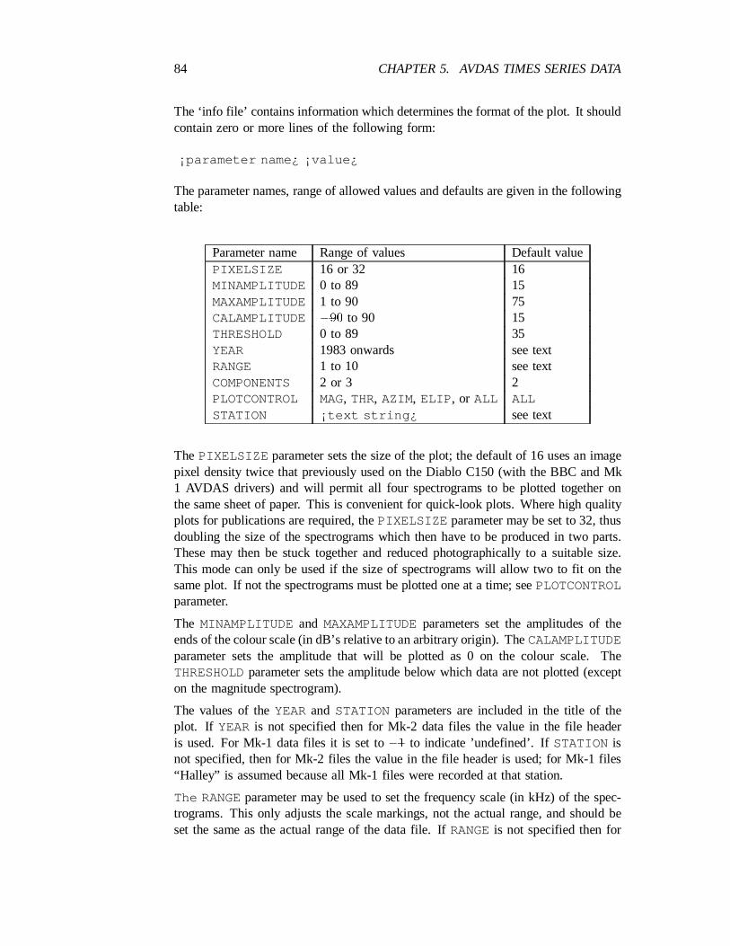
84 CHAPTER 5. AVDAS TIMES SERIES DATA
The ‘info file’ contains information which determines the format of the plot. It shouldcontain zero or more lines of the following form:
¡parameter name¿ ¡value¿
The parameter names, range of allowed values and defaults are given in the followingtable:
Parameter name Range of values Default valuePIXELSIZE 16 or 32 16MINAMPLITUDE 0 to 89 15MAXAMPLITUDE 1 to 90 75CALAMPLITUDE ¡90 to 90 15THRESHOLD 0 to 89 35YEAR 1983 onwards see textRANGE 1 to 10 see textCOMPONENTS 2 or 3 2PLOTCONTROL MAG, THR, AZIM, ELIP , or ALL ALLSTATION ¡text string¿ see text
ThePIXELSIZE parameter sets the size of the plot; the default of 16 uses an imagepixel density twice that previously used on the Diablo C150 (with the BBC and Mk1 AVDAS drivers) and will permit all four spectrograms to be plotted together onthe same sheet of paper. This is convenient for quick-look plots. Where high qualityplots for publications are required, thePIXELSIZE parameter may be set to 32, thusdoubling the size of the spectrograms which then have to be produced in two parts.These may then be stuck together and reduced photographically to a suitable size.This mode can only be used if the size of spectrograms will allow two to fit on thesame plot. If not the spectrograms must be plotted one at a time; seePLOTCONTROLparameter.
The MINAMPLITUDEand MAXAMPLITUDEparameters set the amplitudes of theends of the colour scale (in dB’s relative to an arbitrary origin). TheCALAMPLITUDEparameter sets the amplitude that will be plotted as 0 on the colour scale. TheTHRESHOLDparameter sets the amplitude below which data are not plotted (excepton the magnitude spectrogram).
The values of theYEARand STATION parameters are included in the title of theplot. If YEARis not specified then for Mk-2 data files the value in the file headeris used. For Mk-1 data files it is set to¡1 to indicate ’undefined’. IfSTATION isnot specified, then for Mk-2 files the value in the file header is used; for Mk-1 files“Halley” is assumed because all Mk-1 files were recorded at that station.
The RANGEparameter may be used to set the frequency scale (in kHz) of the spec-trograms. This only adjusts the scale markings, not the actual range, and should beset the same as the actual range of the data file. IfRANGEis not specified then for
5.16. ANALYSIS SOFTWARE 85
Mk-2 data files, or 3-component Mk-1 data files, the value in the file header is used.For 2-component Mk-1 data files the default is 10 kHz.
For Mk-1 data files theCOMPONENTSparameter must match the number of compo-nents in the file. It may only take the values 2 or 3 and defaults to 2. This parameteris not used with Mk-2 data files.
The PLOTCONTROLparameter determines which spectrograms are plotted. It maytake the valuesMAG, THR, AZIM, ELIP or ALL and defaults toALL.
As an example, Fig. 5.1 was produced by the command:
DSPPLOT TS89221L.DAT INFO89.PLT TS89221L.GRF
where the ‘info file’ INFO89.PLT is:
YEAR 1989RANGE 10COMPONENTS 2
5.16.5 DSP3CP
The programmeDSP3CPis intended for processing three component DSP calibrationframes or any other three-component DSP frames containing constant frequency sig-nals. The output from the programme gives estimates of the frequency of the signal,the amplitude of each of the three components, and the phase ofH andH relativex y
to E . It can use a calibration file, produced by previously running the programmez
on a set of calibration frames, to correct for the amplitude and phase response of thereceiver.
The programme is run using a command of the following form.
DSP3CP ¡control file¿ [+C=¡cal file¿] [+0=¡output file¿]
The control file should contain one line for each frequency to be measured. Eachline should contain the following data.
¡data file name¿ ¡frequency¿ ¡Ez ref¿ ¡Hx ref¿ ¡Hy ref¿
The data file name would normally be the name of the file containing the data to beprocessed. However, when a single file contains signals of several frequencies (suchas the multi-frequency calibration tone), the file name should only be specified forthe first frequency. For the other frequencies a* should be used instead.
The frequency specified should be the approximate frequency of the signal to bemeasured. The programme will search a small range centred on this frequency.
If the frequency specified is above the frequency range of the data file, the programmewill assume that the required signal is recorded as an alias and correct the measured
86 CHAPTER 5. AVDAS TIMES SERIES DATA
frequency and phase accordingly. If a calibration file is being used then all signalsinvolved, both in the control file and the calibration file, must either be aliased ornon-aliased.
The three ‘ref’ parameters are subtracted from the amplitudes of the three signalcomponents. When the programme is being used to measure signal amplitudes, theanalogue gains (in dB) would normally be entered as the ‘ref’ parameters.
If the programme is being used to produce a calibration file, the ‘ref’ parametersshould be the equivalent received signal strength of the calibration signal plus the
¡33 2 ¡1analogue gains. The amplitude should be measured in dB relative to10 T Hzusing a nominal bandwidth of 100 Hz (1 pT = 70.0 on this scale). TheH andHx y
±calibration signals are¡3 dB wrt 1 pT (since the calibration coil is at 45 ) and ananalogue gain of 10 dB is normally used. TheH andH ‘refs’ would therefore bex y
entered as 77.0.
The most recent estimate of the equivalent field strength of theE calibration signalz
is 3.7 dB wrt 1 pT. This is recorded with an analogue gain of 0 dB and so theEz
‘ref’ would be entered as 73.7.
The following is a sample of a control file (CALCONTused to process the calibrationsrecorded in February 1986).
TSC86057.DAT 300.0 73.7 77.0 77.0TSC86058.dat 400.0 73.7 77.0 77.0TSC86059.DAT 500.0 73.7 77.0 77.0TSC86060.DAT 600.0 73.7 77.0 77.0TSC86061.DAT 700.0 73.7 77.0 77.0TSC86062.DAT 800.0 73.7 77.0 77.0TSC86063.DAT 1000.0 73.7 77.0 77.0
The programme would be run as follows to produce a calibration file.
DSP3CP CALCONT +0=CALFILE
The output from the programme should look like this.
31 12 0 17 301.6 -24.5 -22.5 -21.9 -29.5 150.931 12 1 42 403.4 -22.2 -19.1 -18.7 -15.3 168.331 12 2 47 500.8 -20.6 -16.9 -16.7 -0.5 -179.831 12 4 4 594.3 -19.1 -15.9 -15.5 7.0 -169.431 12 5 1 699.8 -18.1 -14.8 -14.6 17.9 -159.731 12 5 58 795.7 -17.4 -14.3 -14.1 27.2 -151.031 12 7 6 1004.2 -16.2 -13.8 -13.9 40.7 -138.1
To check if the programme is working properly it can be run again using a calibrationfile.
DSP3CP CALCONT +C=CALFILE +0=CALCHECK
The amplitudes and phases should be close to zero.
5.16. ANALYSIS SOFTWARE 87
31 12 0 17 296.2 -0.5 -0.8 -0.6 -2.9 -3.631 12 1 42 398.4 -0.2 -0.2 -0.2 -1.7 -1.131 12 2 47 497.3 0.0 0.0 0.1 0.7 0.231 12 4 4 592.1 0.2 0.2 0.2 1.0 1.631 12 5 1 697.9 0.1 0.2 0.2 2.1 1.831 12 5 58 795.0 -0.1 -0.0 0.0 -0.8 -0.831 12 7 6 1003.9 -0.0 0.0 -0.0 -0.2 -0.2
5.16.6 SIMULATE
This programme simulates the data that would be received from a single ellipticallypolarised wave using a perfect receiver. It is run using the following command:
SIMULATE file_name A B theta phi freq
where file_name is the name of the file to contain the simulated data,A and Bare the amplitudes (in ADC units) of the major and minor axes of the polarisationellipse, theta andphi are the azimuth and zenith angle of the received wave, andfreq is the frequency in bin numbers (maximum 127).
5.16.7 DSP3SPEC
DSP3SPECis a programme to produce a file of complex spectra from (old format)3-component DSP data. It will accept a calibration file in the format used byDSP3CPto correct the amplitude and phase response of the receiver.
The phases of each point in the spectra are adjusted to make the phase ofE zeroz
(the same adjustment being applied toH andH ). This means that the phase of thex y
H andH spectra indicates the phase of theH andH components relative toE .x y x y z
Each spectrum is output in real and imaginary form (except for the imaginary part ofE which is always zero) as a series of 128 integers written on one line. A token atz
the beginning of the line identifies the component. A total of five lines are output foreach block of data in the time series file; these areE real,H real,H imaginary,z x x
H real,H imaginary. The convention used here is thatH is the signal from they y x
North-South (A) loop andH is the signal from the West-East (B) loop.y
A header at the beginning of the output file indicates the name of the time series fileused, the day and time the data were recorded, the frequency range, the number ofblocks and the reference level (ref_level ). Absolute amplitudes in dB relative tothe standard amplitude reference (used to prepare the calibration file) may be obtainedusing the following formula.
10£ log 10(<£<+=£=)¡ ref level
(< and= are the integer amplitudes of the required spectrum point).
The programme is run using the following command:
88 CHAPTER 5. AVDAS TIMES SERIES DATA
DSP3SPEC input_file output_file [options]
where theoptions may be any of:
+C=cal_file
+Z=Ez_ref
+X=Hx_ref
+Y=Hy_ref
The ref ’s are the gain settings (in dB) of the low-pass filters when the data wererecorded (nominally 0, 10 or 20). They are used in the same way as theref ’sspecified in the control file toDSP3CP(see section above).
5.16.8 Spectrum files
The main types of derived data sets are spectral files, created by Fourier transformingthe time series data.
The original formats of the spectral files are described in the 1983 Halley VLF reportby Keith Yearby. There are three types of spectral file: complex spectral amplitude,compressed cross-spectrum (CCS) and compressed auto (power) spectrum (CPS).The latter is the format of the files produced by the AVDASSAVEcommand (seeSection 1.15.1). The purpose of the compressed files was to save transmission costsof sending the files over the satellite data link from Halley.
5.16.9 Complex spectral amplitude files
Like the time series data files, complex spectra files (filenames of the typeDSP-SAnn.DATwherenn is the same as the corresponding time series file) are again binary data files,with the first 4 bytes containing the frame time. The rest of the file contains 127spectra of 128 points each, with each point encoded using 4 bytes. Each point in thespectrum is a vector whose magnitude represents the total power received by the aeri-als, and whose components represent the distribution of the power between differentwave polarisations and signal directions. In cartesian co-ordinates the components
2 2 ¤ ¤arex = (jAj ¡ jBj )=2, y = <(AB ), z = =(AB ). The three components and2 2the average powerp = (jAj + jBj )=2 are summed over two FFT spectra to make
one spectrum in the file. HereA andB are the complex spectral amplitude for the Aand B loops. The 4 bytes in the file for each spectrum point areLOGMAG, THETA,PHI andCOHER. The first three represent thex; y; z components of the spectrum ina spherical polar co-ordinate formr; µ; Á.
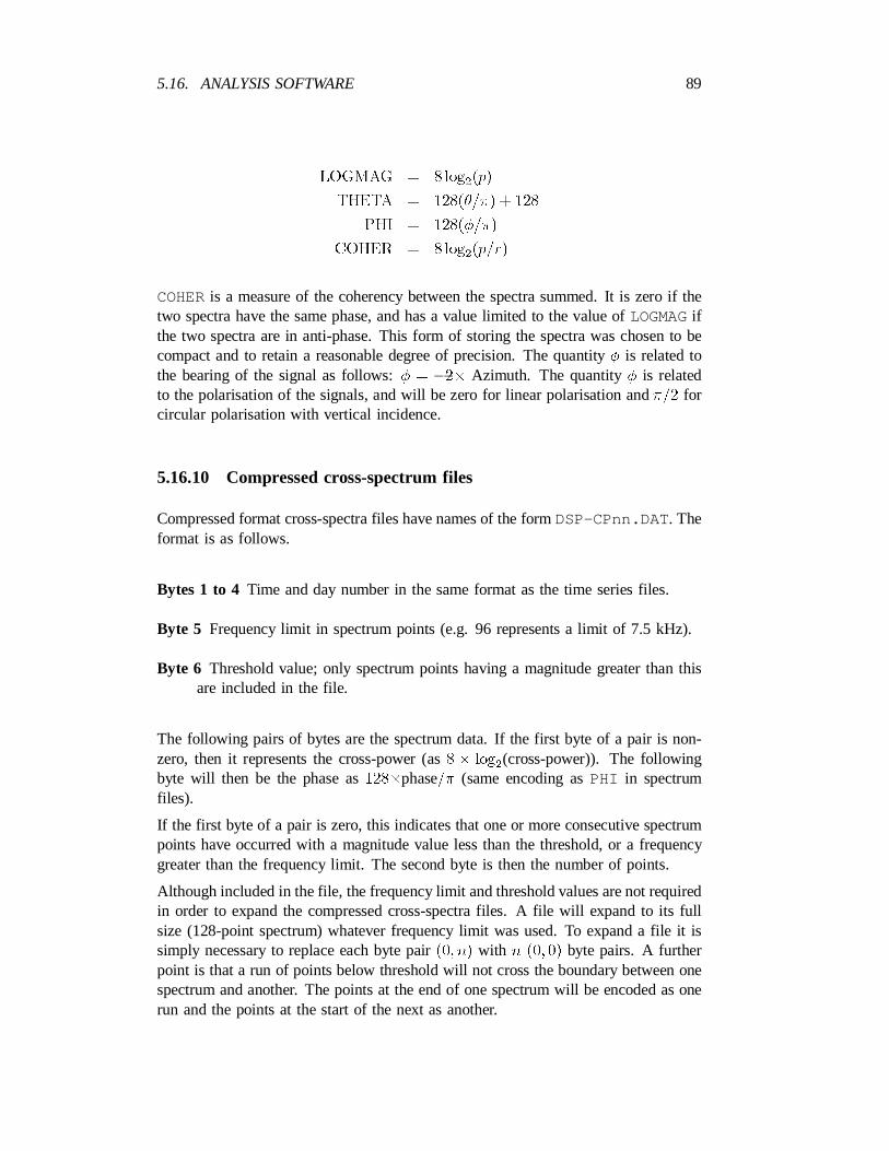
5.16. ANALYSIS SOFTWARE 89
LOGMAG = 8 log (p)2
THETA = 128(µ=¼) + 128
PHI = 128(Á=¼)
COHER = 8 log (p=r)2
COHERis a measure of the coherency between the spectra summed. It is zero if thetwo spectra have the same phase, and has a value limited to the value ofLOGMAGifthe two spectra are in anti-phase. This form of storing the spectra was chosen to becompact and to retain a reasonable degree of precision. The quantityÁ is related tothe bearing of the signal as follows:Á = ¡2£ Azimuth. The quantityÁ is relatedto the polarisation of the signals, and will be zero for linear polarisation and¼=2 forcircular polarisation with vertical incidence.
5.16.10 Compressed cross-spectrum files
Compressed format cross-spectra files have names of the formDSP-CPnn.DAT. Theformat is as follows.
Bytes 1 to 4 Time and day number in the same format as the time series files.
Byte 5 Frequency limit in spectrum points (e.g. 96 represents a limit of 7.5 kHz).
Byte 6 Threshold value; only spectrum points having a magnitude greater than thisare included in the file.
The following pairs of bytes are the spectrum data. If the first byte of a pair is non-zero, then it represents the cross-power (as8 £ log (cross-power)). The following2
byte will then be the phase as128£phase=¼ (same encoding asPHI in spectrumfiles).
If the first byte of a pair is zero, this indicates that one or more consecutive spectrumpoints have occurred with a magnitude value less than the threshold, or a frequencygreater than the frequency limit. The second byte is then the number of points.
Although included in the file, the frequency limit and threshold values are not requiredin order to expand the compressed cross-spectra files. A file will expand to its fullsize (128-point spectrum) whatever frequency limit was used. To expand a file it issimply necessary to replace each byte pair(0; n) with n (0; 0) byte pairs. A furtherpoint is that a run of points below threshold will not cross the boundary between onespectrum and another. The points at the end of one spectrum will be encoded as onerun and the points at the start of the next as another.
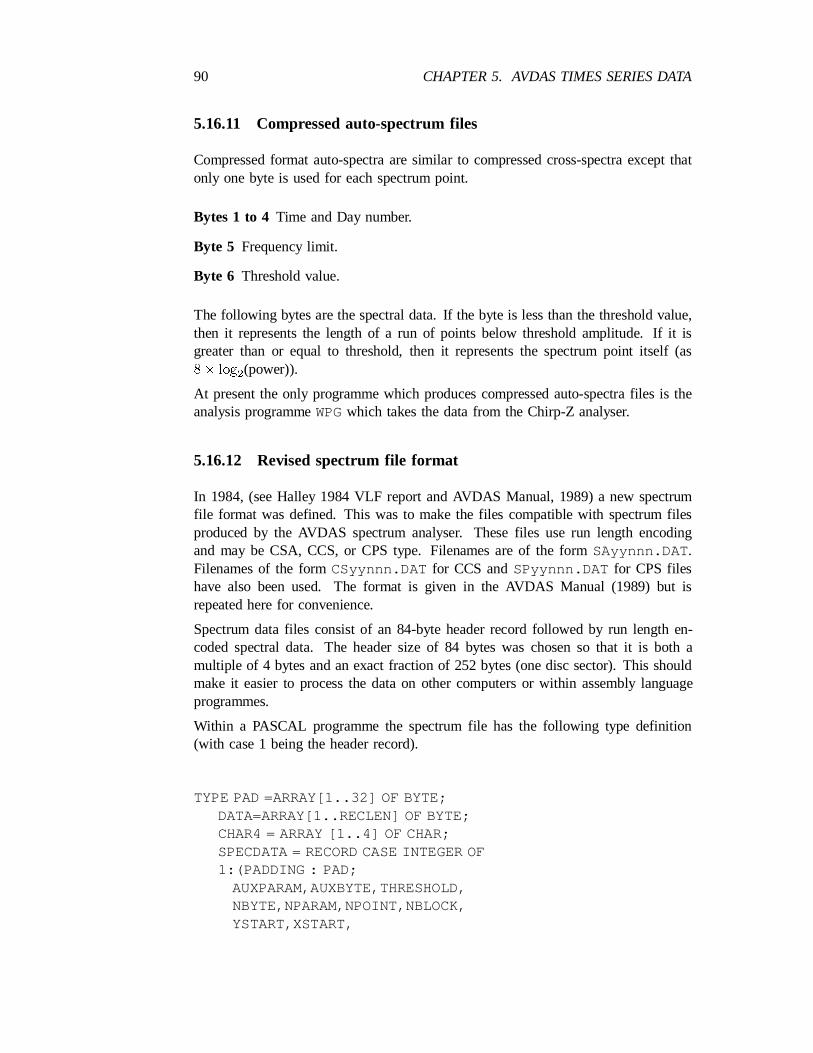
90 CHAPTER 5. AVDAS TIMES SERIES DATA
5.16.11 Compressed auto-spectrum files
Compressed format auto-spectra are similar to compressed cross-spectra except thatonly one byte is used for each spectrum point.
Bytes 1 to 4 Time and Day number.
Byte 5 Frequency limit.
Byte 6 Threshold value.
The following bytes are the spectral data. If the byte is less than the threshold value,then it represents the length of a run of points below threshold amplitude. If it isgreater than or equal to threshold, then it represents the spectrum point itself (as8£ log (power)).2
At present the only programme which produces compressed auto-spectra files is theanalysis programmeWPGwhich takes the data from the Chirp-Z analyser.
5.16.12 Revised spectrum file format
In 1984, (see Halley 1984 VLF report and AVDAS Manual, 1989) a new spectrumfile format was defined. This was to make the files compatible with spectrum filesproduced by the AVDAS spectrum analyser. These files use run length encodingand may be CSA, CCS, or CPS type. Filenames are of the formSAyynnn.DAT .Filenames of the formCSyynnn.DAT for CCS andSPyynnn.DAT for CPS fileshave also been used. The format is given in the AVDAS Manual (1989) but isrepeated here for convenience.
Spectrum data files consist of an 84-byte header record followed by run length en-coded spectral data. The header size of 84 bytes was chosen so that it is both amultiple of 4 bytes and an exact fraction of 252 bytes (one disc sector). This shouldmake it easier to process the data on other computers or within assembly languageprogrammes.
Within a PASCAL programme the spectrum file has the following type definition(with case 1 being the header record).
TYPE PAD =ARRAY[1..32] OF BYTE;DATA=ARRAY[1..RECLEN] OF BYTE;CHAR4 = ARRAY [1..4] OF CHAR;SPECDATA = RECORD CASE INTEGER OF1:(PADDING : PAD;
AUXPARAM,AUXBYTE,THRESHOLD,NBYTE,NPARAM,NPOINT,NBLOCK,YSTART,XSTART,
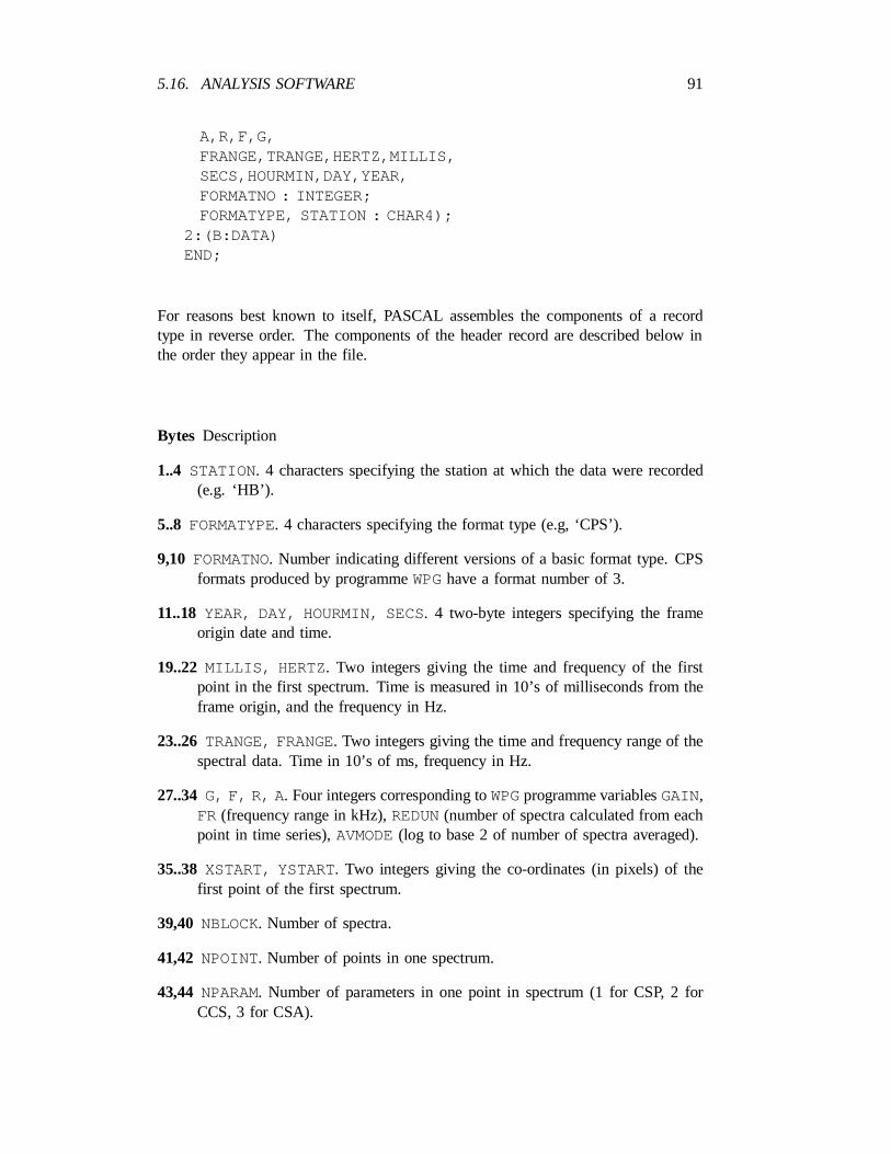
5.16. ANALYSIS SOFTWARE 91
A,R,F,G,FRANGE,TRANGE,HERTZ,MILLIS,SECS,HOURMIN,DAY,YEAR,FORMATNO : INTEGER;FORMATYPE, STATION : CHAR4);
2:(B:DATA)END;
For reasons best known to itself, PASCAL assembles the components of a recordtype in reverse order. The components of the header record are described below inthe order they appear in the file.
Bytes Description
1..4 STATION. 4 characters specifying the station at which the data were recorded(e.g. ‘HB’).
5..8 FORMATYPE. 4 characters specifying the format type (e.g, ‘CPS’).
9,10 FORMATNO. Number indicating different versions of a basic format type. CPSformats produced by programmeWPGhave a format number of 3.
11..18 YEAR, DAY, HOURMIN, SECS. 4 two-byte integers specifying the frameorigin date and time.
19..22 MILLIS, HERTZ . Two integers giving the time and frequency of the firstpoint in the first spectrum. Time is measured in 10’s of milliseconds from theframe origin, and the frequency in Hz.
23..26 TRANGE, FRANGE. Two integers giving the time and frequency range of thespectral data. Time in 10’s of ms, frequency in Hz.
27..34 G, F, R, A . Four integers corresponding toWPGprogramme variablesGAIN,FR (frequency range in kHz),REDUN(number of spectra calculated from eachpoint in time series),AVMODE(log to base 2 of number of spectra averaged).
35..38 XSTART, YSTART. Two integers giving the co-ordinates (in pixels) of thefirst point of the first spectrum.
39,40 NBLOCK. Number of spectra.
41,42 NPOINT. Number of points in one spectrum.
43,44 NPARAM. Number of parameters in one point in spectrum (1 for CSP, 2 forCCS, 3 for CSA).
92 CHAPTER 5. AVDAS TIMES SERIES DATA
45,46 NBYTE. Number of bytes used to encode each parameter (1 for all formatspresently defined).
47,48 THRESHOLD. Threshold level used for run length encoding.
49..52 AUXBYTE, AUXPARAM. Number of bytes per parameter and number of pa-rameters of auxiliary data that is associated with each spectrum and not subjectto run length encoding.AUXBYTE= 1 for all formats presently defined, andAUXPARAMis normally one for CSP formats and zero for CCS and CSA.However programmes reading these formats should allow for different valuesof AUXPARAMand skip the extra bytes as required.
The following bytes are the spectral data. For CPS files, one byte represents one ormore spectrum points. If the byte is less than the threshold value, then it representsthe length of a run of points below threshold amplitude. If it is greater than or equalto the threshold then it represents the spectrum point itself (as8£ log (power)).
2
For a CCS file, pairs of bytes represent one or more spectrum points. If the first byteof a pair is non-zero then it represents the cross-power (as8 £ log (cross-power)).
2
The following byte will then be the phase (as128 £ phase=¼). If the first byteof a pair is zero, this indicates that one or more consecutive spectrum points haveoccurred with a magnitude value less than the threshold or a frequency greater thanthe frequency limit. The second byte is then the number of points. To expand a fileit is simply necessary to replace each byte pair(0; n) with n (0; 0) byte pairs.
For a CSA file, groups of three bytes represent one or more spectrum points. If thefirst byte of a group is non-zero, then it represents the power (as8£log (power)). The
2
following byte will then be the azimuth (as 128£ azimuth/360), and the third bytethe ellipticity (as 128£ ellipticity). If the first byte of a group is zero, this indicatesthat one or more consecutive spectrum points have occurred with a magnitude valueless than the threshold or a frequency greater than the frequency limit. The secondbyte is then the number of points. To expand a file it is simply necessary to replaceeach byte group(0; n; 0) with n (0; 0; 0) byte groups.
A further point is that a run of points below threshold will not cross the boundarybetween one spectrum and another. The points at the end of one spectrum will beencoded as one run and the points at the start of the next as another.
Filenames with extensions.MAG, .AZM, and.ELP contain magnitude, azimuth, andellipticity data, respectively, derived from the corresponding.DAT file.
5.16.13 Paper plots
These have been produced in colour, one sheet per file, usingDSPPLOT, and a folderexists.
5.17. ARCHIVING 93
5.17 Archiving
The time series data have been transferred to CD-ROM.
5.18 Documentation
² AVDAS Mk-I Manual, by Keith Yearby, 1989. This gives information aboutthe procedure for recording the data, analysing them, and calibrations. It alsocontains the spectrum files formats, and details about obtaining hardcopy.
² VLF Manual (by various authors, updated Keith Yearby, 1989). Gives a de-scription of the basic VLF system as used at Halley.
² UK Analysis Manual(edited by Keith Yearby, 1989). Covers a number oftopics relevant to data analysis in the UK, which are not treated elsewhere.
² Halley VLF Manualedited by A.J. Smith and J. Digby, June 1995.
² DSP-II Digital Signal Processing System: User Manuals(1993) High GreaveAssociates, Sheffield.
5.19 References
5.19.1 Unpublished
² Halley VLF Report 1983, K.H. Yearby, BAS Reference Z/1983/I4.
² Halley VLF Report 1984, K.H. Yearby, BAS Reference Z/1984/I4.
² Halley VLF Report 1985, T.D.G. Clark, BAS Reference Z/1985/I3.
² Halley VLF Report 1986, T.D.G. Clark, BAS Reference Z/1986/I2.
² Halley VLF Report 1989, D. Ingle, BAS Reference Z/1989/I8.
² Halley VLF Report 1995,J. Digby and A. Phillips, BAS Reference Z/1995/I7.
5.19.2 Published
² Cotton P.D. (1989) A study of Antarctic subionospheric propagation at frequen-cies below 10 kHz. Ph.D. thesis, University of Sheffield.
² Ho D. and Bernard L.C. (1973) A fast method to determine the nose frequencyand minimum group delay of a whistler when the causative spheric is unknown.J. Atmos. Terr. Phys. bf 35, 881–887.
94 CHAPTER 5. AVDAS TIMES SERIES DATA
² Jones D. (1984) Antarctic research by satellite link. Nature307, 12–13.
² Park (1972) Methods of determining electron concentrations in the magneto-sphere from nose whistlers. Stanford Electronics Labs. Tech. Rept. No. 3454-1.
² Smith A.J. and Yearby K.H. (1987) AVDAS – A microprocessor-based VLFsignal processing and spectral analysis facility for Antarctica. Br. Antarct. Surv.Bull. 75, 1–15.
² Strangeways H.J. (1980) Systematic errors in VLF direction-finding of whistlerducts – I. J. Atmos. Terr. Phys.42, 995–1008.
² Tarcsai G., Strangeways H.J. and Rycroft M.J. (1989) Error sources and traveltime residuals in plasmaspheric whistler interpretation. J. Atmos. Terr. Phys.51, 249–258.
² Tsuruda K. and Ikeda M. (1979) Comparison of three different types of VLFdirection finding techniques. J. Geophys. Res.84, 5325–5332.
² Yearby K.H. and Smith A.J. (1994) The polarisation of whistlers received onthe ground nearL = 4. J. atmos. terr. Phys.,56, 1499–1512.
Chapter 6
RALF data
6.1 Brief description
Provides simultaneous time series measurements of the earth’s magnetic field and theintensity of naturally occurring VLF emissions.
6.2 Detailed description
RALF is an abbreviation for the Real Time Antarctic Logger Facility. The namederives from the fact that in its original operation, signal processing was used inorder to decide if there were signals present which should be recorded. RALF wasoperative at Halley, Antarctica between January 1986 and January 1991. It wasprimarily designed to look for evidence of correlations between variations of theearth’s magnetic field and similar and simultaneous intensity modulations of VLFradio emissions.
The hardware was based on a BAS 6809 micro-computer system. Logger inputs werethe signals from three orthogonal ULF sensors (X, Y , Z) and the wide band signalfrom a VLF receiver (the main receiver at Halley). The latter was first processed byanalogue band-pass filters and rectifiers to give the amplitude envelope in 3 frequencybands (0.5–1.5 kHz, 2.5–3.5 kHz, 5–7 kHz). The data were recorded on standard9-track computer tape. The frequency response of the ULF sensors lies nominally inthe range 0.1–10 Hz.
RALF was modified several times (leading to successive versions hereafter RALF.1,RALF.2 and RALF.3) after its installation in 1986. These modifications were con-cerned with the amount and rate of data recorded; the actual pass-bands of the VLFand ULF channels were unchanged throughout. Central to the original project designwas the 2-speed recording system designed to offer a saving on data analysis andstorage by the use of real-time in-stream data analysis designed to record at highspeed only those events judged to be of interest.
95
96 CHAPTER 6. RALF DATA
Originally (RALF.1), in low speed (the normal recording mode) the 3 VLF channelswere recorded at 1 Hz, with the maximum fluctuation every 10 s in the 3 ULFchannels. In high-speed mode data were recorded in both the VLF and ULF channelsat 20 Hz. The logger was later modified to also record continuously at low speedin the 3 ULF channels (RALF.2). In the final version (RALF.3) the event detectionroutines were not used and a continuous ‘low-speed’ of 10 Hz was recorded in all 6channels.
In RALF.1 and 2 the high speed recordings could be started by a direct command fromthe operator (or at a preset time specified by the operator up to 24 hours in advance),or by the automatic event-detection routines. Selection of the high-speed mode by theoperator was also possible in version 3. Triggering of high speed recording occurredwhen the amplitude fluctuations in the ULF channels exceeded preset levels (the VLFchannels were not used as they can be triggered erroneously by man-made signalsor spherics), or when the cross-correlations continuously being performed betweenthe VLF and ULF channels exceeded a preset level of significance. In each case,recording reverted to low-speed mode after a set length of time had elapsed (typically20 minutes from the last time a significance level was exceeded).
6.3 Instrument/sensor
6.3.1 Hardware
The data logger hardware was based on a ‘BAS micro’ fitted with a 13-slot digital1bus, a 7-slot analogue bus and two 5 inch floppy disc drives. A Thorn EMI 9-track4
magnetic tape deck was used for recording the data.
The programmable filter-amplifier cards were a general-purpose card used in severalBAS data loggers (e.g. the magnetometer and riometer logger) and are described inseparate documentation.
VLF Filter Cards
The VLF filter cards took a wide-band VLF signal and produced an output propor-tional to the signal amplitude in the required band. The signal first passed through a3-stage band pass filter. The centre frequencyf , gain andQ of each stage, for each0
channel, are given below. The mean level at the output of the rectifier was equal tothe peak-to-peak signal level at the input of the buffer.
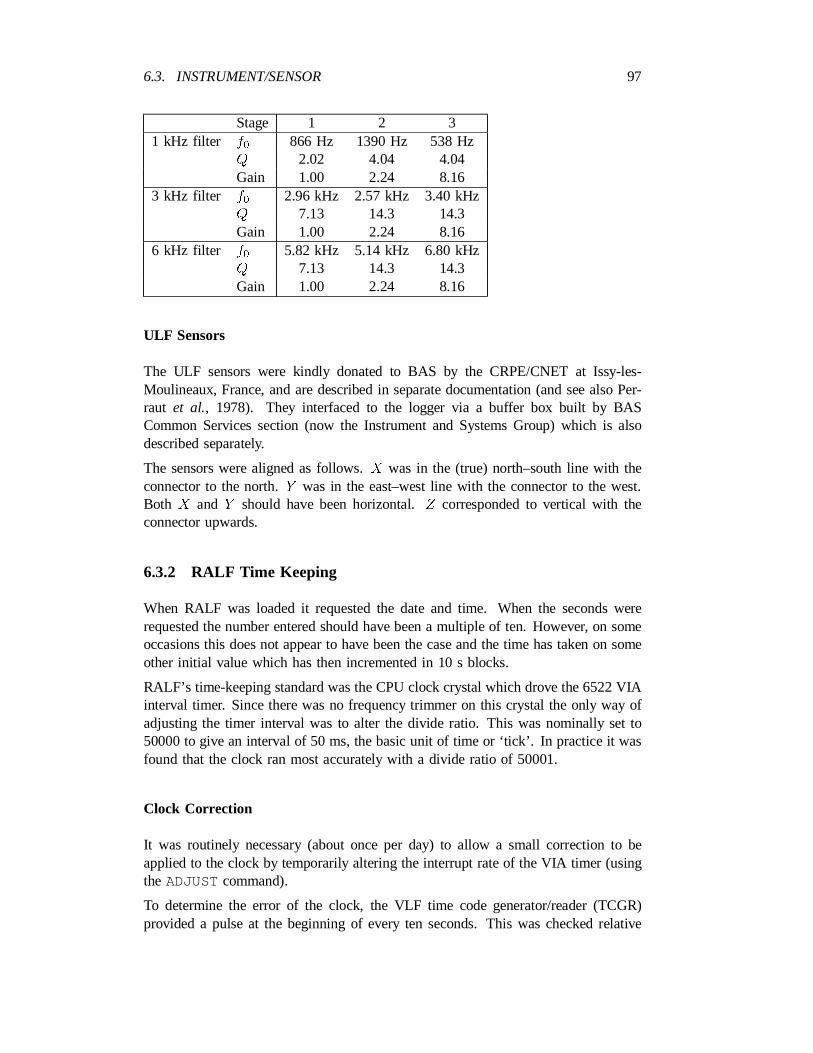
6.3. INSTRUMENT/SENSOR 97
Stage 1 2 31 kHz filter f 866 Hz 1390 Hz 538 Hz0
Q 2.02 4.04 4.04Gain 1.00 2.24 8.16
3 kHz filter f 2.96 kHz 2.57 kHz 3.40 kHz0
Q 7.13 14.3 14.3Gain 1.00 2.24 8.16
6 kHz filter f 5.82 kHz 5.14 kHz 6.80 kHz0
Q 7.13 14.3 14.3Gain 1.00 2.24 8.16
ULF Sensors
The ULF sensors were kindly donated to BAS by the CRPE/CNET at Issy-les-Moulineaux, France, and are described in separate documentation (and see also Per-raut et al., 1978). They interfaced to the logger via a buffer box built by BASCommon Services section (now the Instrument and Systems Group) which is alsodescribed separately.
The sensors were aligned as follows.X was in the (true) north–south line with theconnector to the north.Y was in the east–west line with the connector to the west.Both X and Y should have been horizontal.Z corresponded to vertical with theconnector upwards.
6.3.2 RALF Time Keeping
When RALF was loaded it requested the date and time. When the seconds wererequested the number entered should have been a multiple of ten. However, on someoccasions this does not appear to have been the case and the time has taken on someother initial value which has then incremented in 10 s blocks.
RALF’s time-keeping standard was the CPU clock crystal which drove the 6522 VIAinterval timer. Since there was no frequency trimmer on this crystal the only way ofadjusting the timer interval was to alter the divide ratio. This was nominally set to50000 to give an interval of 50 ms, the basic unit of time or ‘tick’. In practice it wasfound that the clock ran most accurately with a divide ratio of 50001.
Clock Correction
It was routinely necessary (about once per day) to allow a small correction to beapplied to the clock by temporarily altering the interrupt rate of the VIA timer (usingthe ADJUSTcommand).
To determine the error of the clock, the VLF time code generator/reader (TCGR)provided a pulse at the beginning of every ten seconds. This was checked relative
98 CHAPTER 6. RALF DATA
to the start of the current 10 second data block. This information will have beenincluded in the data written to tape and so can be used during analysis to determineaccurately the time of the data. This did rely on the error of the VLF TCGR beingaccurately known (which it normally is to§10 ms) and that the TCGR was workingin ‘generator’ rather than ‘reader’ mode. As the latter was not always the case, anaccurate log should have been kept of when the clock error information was invalid.
To avoid discontinuities in the time marking of the recorded data the corrections wereapplied gradually by temporarily altering the divide ratio of the VIA. An increase ordecrease of one part in 10000 was used and this was maintained for a length of time10000 times the correction required. This was done using theADJUSTcommand.For a correction greater then§3:2 s it will have been necessary to close the tapefirst (using theCLOSEcommand) and enter a new date and time (using theTIMEcommand).
6.3.3 Software Description
RALF.3 is a revised version of RALF.2, which is a revised version of RALF.1.The data collection task and the clock task have had only fairly minor revisionsbetween versions and the system for handling the data buffers has been retained. Thedata processing task and the user service task have had major revisions. The eventdetection routines were not used in RALF.3
The RALF programme contains a package of assembly language procedures (ASMPROC)for performing tasks which can be done easier or faster in assembler than in a highlevel language. The input data was restricted to the sub-range¡11 to +11 (resultwill be rubbish if it was not) and sum of products (16 bit integer) returned directly(no division performed).
The low-pass filtering is done using a 19-point transversal filter with a Kaiser-typewindow. One output data point is calculated for every 2 input data points. Theoperation is done using all 16 bits of the input data although the filter coefficientsare only 8-bit quantities.
6.4 Recording method
6.4.1 Event Detection Routines
The logger should normally have been operated in auto-gain mode, although manualgain was available for special occasions such as calibrations. The logger couldbe manually set to high-speed mode with theRECORDcommand. The automaticevent detection routines worked (in RALF.1 and RALF.2) by triggering high-speedrecording whenever the cross-correlations, or signal amplitude in any of the 3 ULFchannels, exceeded a threshold level.
6.4. RECORDING METHOD 99
Cross-correlations
The cross-correlation functions were continually performed between each VLF andeach ULF channel 10 s data blocks. That is a total of 9 computations in1(kHz)¡X(sensor),3¡X , 6 ¡X, 1 ¡ Y , 3¡ Y , 6 ¡ Y , 1¡ Z , 3 ¡ Z, 6¡ Z. The correlations wereperformed by first calculating, and subtracting out, the mean value of each input dataseries. The data were then scaled by dividing them by two as many times as neces-sary to bring them in the range¡11 to +11 (a particularly fast signed multiplicationoperation is possible for data within this range). The multiplications and summationsrequired to calculate each point in the cross-correlation function were then performed.The zero-lag auto-correlation of each input data series is also calculated so that themaximum amplitude of the correlation function can be normalised with respect toinput signal amplitude variations. The maximum amplitude is given as a numberbetween 0 and 100 representing the degree of correlation between signals.
Amplitude Thresholds
In addition to the triggering by the cross correlations, high-speed recording was startedif a single ULF channel amplitude exceeded a pre-set threshold. The ULF signalswere calculated by finding the peak-to-peak amplitude of the low-pass filtered inputsignal. This value was then converted to dB. The VLF signal levels were calculatedusing the mean of the 200 data points in each 10 s data block, thus providing adegree of rejection of the spherics which often dominate the VLF spectrum. Thethresholds were required to be set appropriately to keep spurious triggerings down toan acceptable level. Because of the problem with spherics in the VLF data producingtriggering by sudden large amplitude signals, the VLF amplitude levels were not usedas high-speed triggers.
6.4.2 Tape Control Commands
The commands for tape operations are listed below.
OPENOpened the magnetic tape for recording. This command assumed that the tapewas correctly positioned for recording to start immediately. It would normallyhave been used when starting a new tape. In other circumstances the commandsREOPENor FINDENDwill have been used.
CLOSEClosed the magnetic tape. This command caused all the saved data buffersto be dumped to the tape followed by a double file mark. The tape will thenhave back-spaced over the file marks so that they may have been found usingREOPEN.
REOPENThis command was used to re-open a partially used tape. The tape willhave spaced through until a double file mark was found and then back spacedover the second file mark.
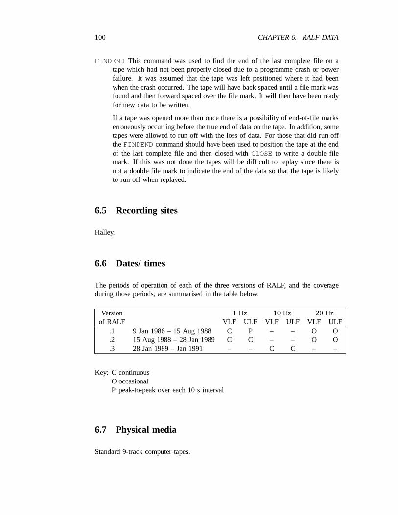
100 CHAPTER 6. RALF DATA
FINDEND This command was used to find the end of the last complete file on atape which had not been properly closed due to a programme crash or powerfailure. It was assumed that the tape was left positioned where it had beenwhen the crash occurred. The tape will have back spaced until a file mark wasfound and then forward spaced over the file mark. It will then have been readyfor new data to be written.
If a tape was opened more than once there is a possibility of end-of-file markserroneously occurring before the true end of data on the tape. In addition, sometapes were allowed to run off with the loss of data. For those that did run offtheFINDENDcommand should have been used to position the tape at the endof the last complete file and then closed withCLOSEto write a double filemark. If this was not done the tapes will be difficult to replay since there isnot a double file mark to indicate the end of the data so that the tape is likelyto run off when replayed.
6.5 Recording sites
Halley.
6.6 Dates/ times
The periods of operation of each of the three versions of RALF, and the coverageduring those periods, are summarised in the table below.
Version 1 Hz 10 Hz 20 Hzof RALF VLF ULF VLF ULF VLF ULF
.1 9 Jan 1986 – 15 Aug 1988 C P – – O O
.2 15 Aug 1988 – 28 Jan 1989 C C – – O O
.3 28 Jan 1989 – Jan 1991 – – C C – –
Key: C continuousO occasionalP peak-to-peak over each 10 s interval
6.7 Physical media
Standard 9-track computer tapes.
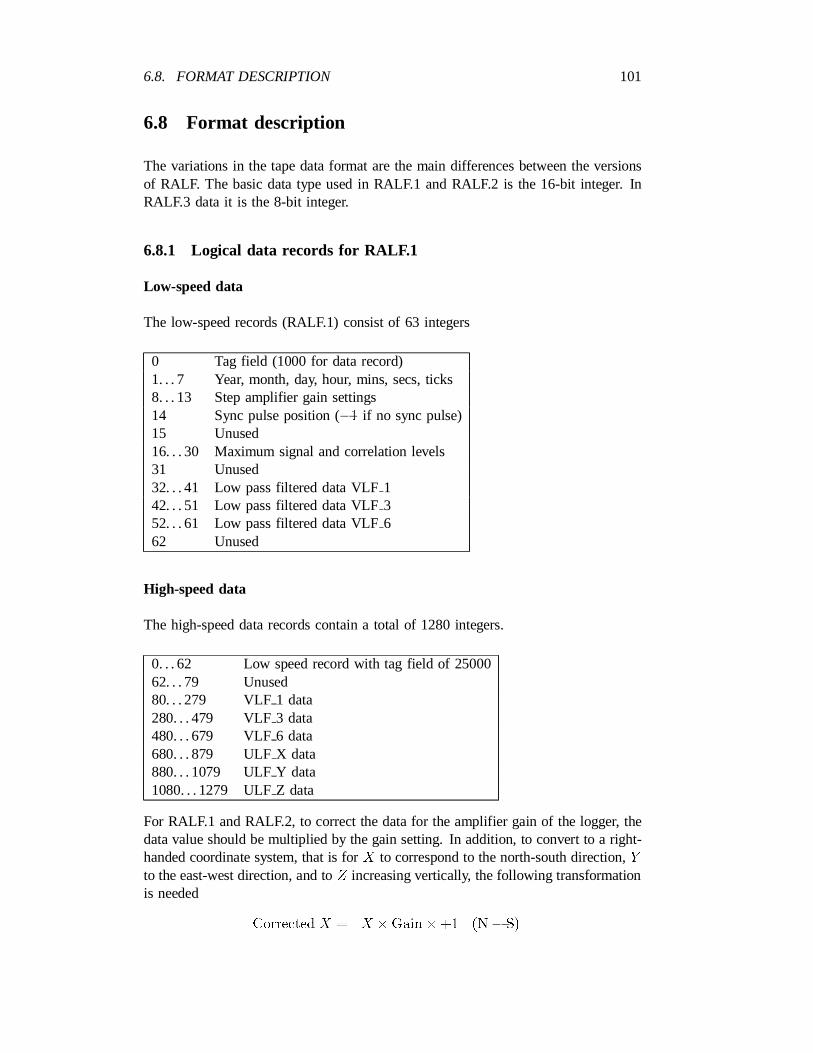
6.8. FORMAT DESCRIPTION 101
6.8 Format description
The variations in the tape data format are the main differences between the versionsof RALF. The basic data type used in RALF.1 and RALF.2 is the 16-bit integer. InRALF.3 data it is the 8-bit integer.
6.8.1 Logical data records for RALF.1
Low-speed data
The low-speed records (RALF.1) consist of 63 integers
0 Tag field (1000 for data record)1. . . 7 Year, month, day, hour, mins, secs, ticks8. . . 13 Step amplifier gain settings14 Sync pulse position (¡1 if no sync pulse)15 Unused16. . . 30 Maximum signal and correlation levels31 Unused32. . . 41 Low pass filtered data VLF 142. . . 51 Low pass filtered data VLF 352. . . 61 Low pass filtered data VLF 662 Unused
High-speed data
The high-speed data records contain a total of 1280 integers.
0. . . 62 Low speed record with tag field of 2500062. . . 79 Unused80. . . 279 VLF 1 data280. . . 479 VLF 3 data480. . . 679 VLF 6 data680. . . 879 ULF X data880. . . 1079 ULF Y data1080. . . 1279 ULF Z data
For RALF.1 and RALF.2, to correct the data for the amplifier gain of the logger, thedata value should be multiplied by the gain setting. In addition, to convert to a right-handed coordinate system, that is forX to correspond to the north-south direction,Y
to the east-west direction, and toZ increasing vertically, the following transformationis needed
CorrectedX = X £Gain£+1 (N¡ S)
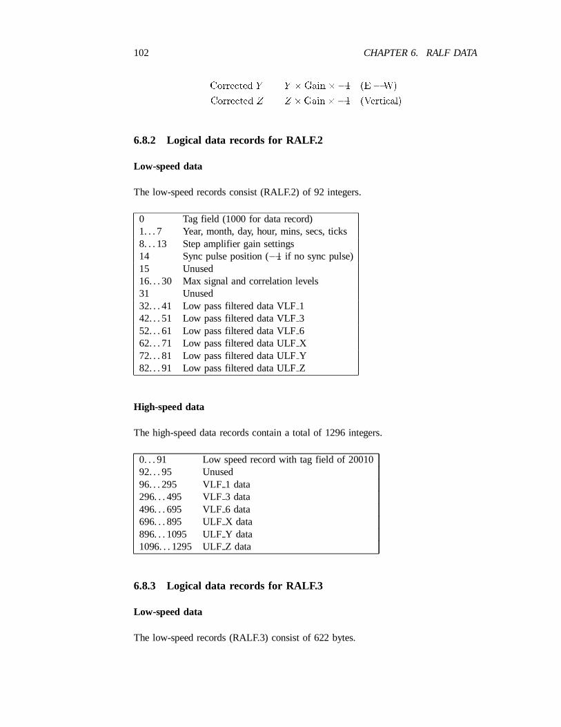
102 CHAPTER 6. RALF DATA
Corrected Y = Y £Gain£¡1 (E¡W)
Corrected Z = Z £Gain£¡1 (Vertical)
6.8.2 Logical data records for RALF.2
Low-speed data
The low-speed records consist (RALF.2) of 92 integers.
0 Tag field (1000 for data record)1. . . 7 Year, month, day, hour, mins, secs, ticks8. . . 13 Step amplifier gain settings14 Sync pulse position (¡1 if no sync pulse)15 Unused16. . . 30 Max signal and correlation levels31 Unused32. . . 41 Low pass filtered data VLF 142. . . 51 Low pass filtered data VLF 352. . . 61 Low pass filtered data VLF 662. . . 71 Low pass filtered data ULF X72. . . 81 Low pass filtered data ULF Y82. . . 91 Low pass filtered data ULF Z
High-speed data
The high-speed data records contain a total of 1296 integers.
0. . . 91 Low speed record with tag field of 2001092. . . 95 Unused96. . . 295 VLF 1 data296. . . 495 VLF 3 data496. . . 695 VLF 6 data696. . . 895 ULF X data896. . . 1095 ULF Y data1096. . . 1295 ULF Z data
6.8.3 Logical data records for RALF.3
Low-speed data
The low-speed records (RALF.3) consist of 622 bytes.
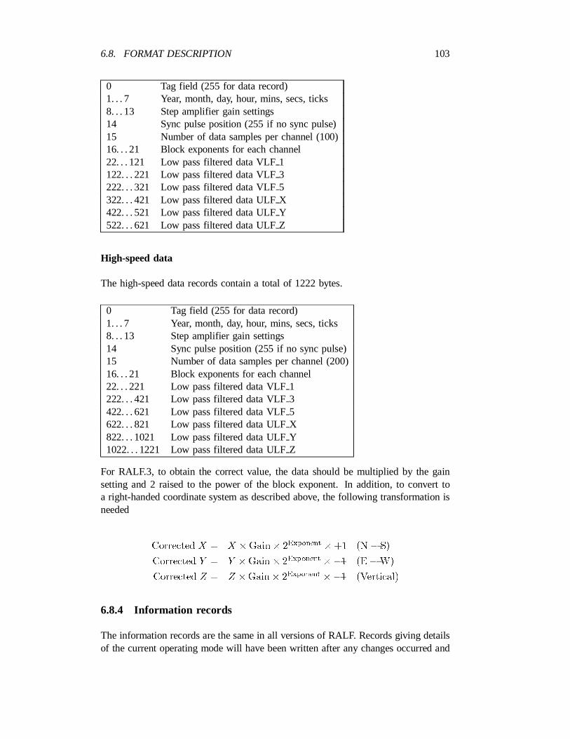
6.8. FORMAT DESCRIPTION 103
0 Tag field (255 for data record)1. . . 7 Year, month, day, hour, mins, secs, ticks8. . . 13 Step amplifier gain settings14 Sync pulse position (255 if no sync pulse)15 Number of data samples per channel (100)16. . . 21 Block exponents foreach channel22. . . 121 Low pass filtered data VLF 1122. . . 221 Low pass filtered data VLF 3222. . . 321 Low pass filtered data VLF 5322. . . 421 Low pass filtered data ULF X422. . . 521 Low pass filtered data ULF Y522. . . 621 Low pass filtered data ULF Z
High-speed data
The high-speed data records contain a total of 1222 bytes.
0 Tag field (255 for data record)1. . . 7 Year, month, day, hour, mins, secs, ticks8. . . 13 Step amplifier gain settings14 Sync pulse position (255 if no sync pulse)15 Number of data samples per channel (200)16. . . 21 Block exponents for each channel22. . . 221 Low pass filtered data VLF 1222. . . 421 Low pass filtered data VLF 3422. . . 621 Low pass filtered data VLF 5622. . . 821 Low pass filtered data ULF X822. . . 1021 Low pass filtered data ULF Y1022. . . 1221 Low pass filtered data ULF Z
For RALF.3, to obtain the correct value, the data should be multiplied by the gainsetting and 2 raised to the power of the block exponent. In addition, to convert toa right-handed coordinate system as described above, the following transformation isneeded
ExponentCorrected X = X £Gain£ 2 £+1 (N¡ S)
ExponentCorrected Y = Y £Gain£ 2 £¡1 (E¡W)
ExponentCorrected Z = Z £Gain£ 2 £¡1 (Vertical)
6.8.4 Information records
The information records are the same in all versions of RALF. Records giving detailsof the current operating mode will have been written after any changes occurred and
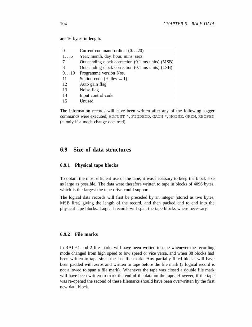
104 CHAPTER 6. RALF DATA
are 16 bytes in length.
0 Current command ordinal (0. . . 20)1. . . 6 Year, month, day, hour, mins, secs7 Outstanding clock correction (0.1 ms units) (MSB)8 Outstanding clock correction (0.1 ms units) (LSB)9. . . 10 Programme version Nos.11 Station code (Halley= 1)12 Auto gain flag13 Noise flag14 Input control code15 Unused
The information records will have been written after any of the following loggercommands were executed;ADJUST *, FINDEND, GAIN * , NOISE, OPEN, REOPEN(* only if a mode change occurred).
6.9 Size of data structures
6.9.1 Physical tape blocks
To obtain the most efficient use of the tape, it was necessary to keep the block sizeas large as possible. The data were therefore written to tape in blocks of 4096 bytes,which is the largest the tape drive could support.
The logical data records will first be preceded by an integer (stored as two bytes,MSB first) giving the length of the record, and then packed end to end into thephysical tape blocks. Logical records will span the tape blocks where necessary.
6.9.2 File marks
In RALF.1 and 2 file marks will have been written to tape whenever the recordingmode changed from high speed to low speed or vice versa, and when 88 blocks hadbeen written to tape since the last file mark. Any partially filled blocks will havebeen padded with zeros and written to tape before the file mark (a logical record isnot allowed to span a file mark). Whenever the tape was closed a double file markwill have been written to mark the end of the data on the tape. However, if the tapewas re-opened the second of these filemarks should have been overwritten by the firstnew data block.
6.10. VALIDATION 105
6.9.3 Decoding logical records
The versions of the fileralfdat.h are ‘C’ structure definitions of the RALF dataformats and need to be included in some C programmes during compilation of the.EXE file.
6.10 Validation
The recorded tapes should all have been replayed on site to check that the recordeddata were valid. They should have been verified withRALFLIST for RALF.1 andRALF.2, andRF3LIST for RALF.3, with option INFO=0 to replay the entire tapeand produce a printer listing of what data had been recorded on it. The programmeshould always terminate with a stop code of¡2 and not give any error messages.When replaying, check also that the tape has in fact replayed up to the point the lastrecording reached (if a spurious double file mark was recorded earlier in the tape itwould stop there).
6.11 Anomalous or suspect data
No information available.
6.12 Calibration
6.12.1 ULF calibrations
The ULF calibration signals were generated using a Farnell FG3 function generatorwhich had been modified to add an extra low frequency range (down to 0.1 Hz).A Hatfield attenuator may have been used in some cases to reduce the level of thesignal applied to the ULF sensors’ internal calibration coils.
6.12.2 VLF Calibrations
The VLF side of the system will have been calibrated in a similar way to the multi-channel VLF receiver (Section 3.12.2). Since we did not have an AF signal generatorwith amplitude modulation capability it was not possible to check the modulationresponse of the VLF channels but this should be well behaved (e.g. flat from zero upto the roll-off of the anti-alias filter).

106 CHAPTER 6. RALF DATA
6.12.3 Procedure
The calibrations were performed on normal data tapes. As with all calibrations theexact timing should have been noted at which each calibration signal was done, andany other times at which the normal recorded data were not valid. In the case ofthe VLF channel calibrations, the configuration of the main VLF receiver (e.g. singlechannel or DSP setup) should have been noted. The quick check calibration shouldnormally have been done every day; the rest of the calibrations twice per year.
6.12.4 Quick check
Done once per day. If possible the calibration should have been done at a time whennatural activity was reasonably quiet. Below is the procedure followed.
1. Set the function generator to give a 1 Hz sine wave of 1 volt peak-to-peakamplitude.
2. Set the attenuator to¡30 dB.
3. Switch the calibration signal through to all three channels. The times shouldhave been noted in the log book.
4. Record for one minute.
5. Repeat (4) for attenuations of¡20, ¡10 and 0 dB.
6.12.5 Frequency response
This part of the calibrations was designed to determine the amplitude and phaseresponses of the sensors as a function of frequency. To allow measurement of phase,the signal generator was also connected directly to the logger by borrowing the inputof one of the sensors not being calibrated. Otherwise the set up for generating thecalibration signals was the same as for the above.
1. Use theGAIN command to set the gain to manual and zero.
2. Set the signal generator to 0.1 Hz (check the frequency with the oscilloscope),1 volt peak-to-peak, attenuator 0 dB.
3. Disconnect the buffer boxZ output from the logger and connect the directoutput from the signal generator in its place.
4. Switch the signal through to channelX .
5. Record 0.1 and 0.15 Hz for two minutes each. Record 0.2, 0.3, 0.5 and 0.7Hz for one minute each. Record 1, 1.5, 2, 3, 5 and 7 Hz for 30 seconds each(including the time taken to change the frequency).
6.12. CALIBRATION 107
6. Repeat step 5 for channelY .
7. Reconnect the buffer boxZ output to the logger; disconnect theX output andconnect the signal generator in its place.
8. Repeat step 5 for channelZ.
9. ReconnectZ output (all sensors connected now).
6.12.6 Sensitivity
This part of the calibrations was to check the sensitivity of the sensors and the relativegain of the programmable gain amplifiers. The logger was operated in auto-gain modewhile the calibration signal amplitude was increased in small increments from a verysmall level up to full scale. It was particularly important that these calibrations weredone when natural activity was low.
1. Use theGAIN command to set auto-gain mode.
2. Set the signal generator to 1 Hz, 1 volt peak-to-peak, attenuator¡75 dB.
3. Switch the signal to all three channels.
4. Record for 30 seconds each at¡75 dB to 0 dB attenuation in 5 dB steps.
6.12.7 Remote source ULF calibrations
The purpose of this part of the calibrations was to provide an independent (fromthe internal calibration coils) check on the sensitivity of the sensors. It is similar inprinciple to the remote source calibration of the VLF receiver. The procedure was asfollows.
1. Set up the large coil 10 m from theX sensor such that the plane of the coilis centred on and perpendicular to the axis of the sensor (this will probablyrequire putting it in a hole in the snow).
2. Set the current (1 amp is equivalent to 1 volt at the current monitor output) fora field strength at the sensor of 1 nT peak-to-peak.
3. Make recordings as for step 5 of the above calibrations.
4. Repeat for theY sensor.
108 CHAPTER 6. RALF DATA
6.12.8 VLF Channel Frequency Responses
This part of the calibrations was to measure the overall frequency response of theVLF side of the system. Unmodulated calibration signals were used and so they willhave been seen by the logger as essentially steady levels. The logger should havebeen operated in manual gain mode on setting one (12 dB). The calibration signalswere injected to the system at the remote receiver hut (CWO) using the same setup as the normal VLF calibrations. The 45 degree calibration coil should have beenused with an equivalent signal strength of 1 pT.
The calibration should have recorded for 30 seconds each at the following frequencies(kHz); 0.25, 0.5, 0.75, 1.0, 1.25, 1.5, 2.0, 2.5, 2.75, 3.0, 3.25, 3.5, 4.0, 5.0, 5.5, 6.0,6.5, 7, 8 and 10.
6.12.9 VLF Channel amplitude response
These calibrations were done using the dummy aerial to inject the calibration signalinto the system. The dual dummy aerial should have been connected to both channelsof the pre-amplifier and the calibration signal connected to channel A of the dummyaerial. The logger should have been be operated in auto-gain mode.
1. Record the dummy aerial noise (with signal generator switched off) for oneminute.
2. Set the signal generator for an equivalent amplitude of¡55 dB ref 1 pT and afrequency of 1 kHz.
3. Record for 30 seconds each at¡55 dB to 0 dB in 5 dB steps.
4. Repeat step 3 for frequencies of 3 kHz and 6 kHz.
6.13 Naming/numbering conventions
The tapes were first labelled at Halley. After return to the UK, all tapes were sentto NERC Computer Services at Keyworth for further use on the Keyworth VAXes(they are now at BAS; see Section 6.18).
6.13.1 Halley Tape Labelling
When a tape was nearly finished the tape was closed with theCLOSEcommand.Tapes were numbered in chronological order for each year (e.g. the tapes for 1988were labelled 88001, 88002, 88003. . . ). Obviously, the time covered byeach tapevaried from tape to tape and version to version. Typically, for RALF.1 and 2 in
6.14. CATALOGUES 109
continuous low speed mode a tape will have lasted for about 6 days, whilst in con-tinuous high speed mode it will have lasted for about 1.5 days. Typically, high speedrecordings are present for one fifth of the time. On average, therefore, a tape lastedseveral days. In RALF.3, with only one recording speed, each tape covers 6 days.
6.13.2 Keyworth Labelling
Until October 1996, the data tapes were stored at Keyworth under user IDU_KMO(Keith Morrison, who worked on the data) for use on the Keyworth VAXes. Theywere assigned new labelsK0**** , where**** was a 4-figure number, by NERCComputing Services. It was necessary to cross reference between Halley logbooksand Keyworth catalogues to match up the tape labelling at Halley and Keyworth. Thetapes were transferred to user IDU_AJS on 20 June 1994.
6.14 Catalogues
Printed catalogues of the tapes exist at BAS tape by tape, year by year (1986–1989).Disc files of the catalogues also exist for 1986, 1987 and 1989. A listing of RALFtapes held at Keyworth could be obtained by use of the VAX commandMYTAPES.
The catalogues for each RALF.1 and 2 tape provide a line listing for each continuoussection of low or high speed data. Each line gives the start and end time of everysection of data, data type (high or low speed), number of records in the section, tapenumber, and finally the sequence numbers of the first and last files in the section. Inthe catalogue listings of RALF.3 tapes the start time, number of samples (100, fromeach 10 s block of data), and records in each file are given for each tape.
6.15 Analysis methods
Programmes written by Keith Yearby were available for the preliminary processingof the RALF data tapes. They were available on the logger itself, and on AVDASand the Keyworth VAXes. The following list is a summary of the programmes. Allprogrammes worked with data recorded on disc (exceptFINDFILE ) and tape (if thecomputer had a tape drive). In the AVDAS and (logger) versions of the programmesthe file name or the device (DEV/MT0 for the tape drive) from which data would beread was specified on the command line when running the programme. On the VAXthe data were always read from logical nameMAGwhich was assigned to a file ortape before running the programme. On both the logger and VAX the tape had to bephysically mounted on the tape drive and the drive switched on-line before runningthe programme.
The master copies of the VAX versions of these programmes were held on the NERCKeyworth VAX in directories[U_KY.SOURCES] and [U_KY.RALFC] , and com-
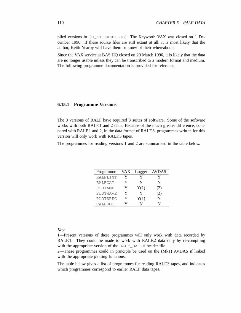
110 CHAPTER 6. RALF DATA
piled versions in[U_KY.EXEFILES] . The Keyworth VAX was closed on 1 De-cember 1996. If these source files are still extant at all, it is most likely that theauthor, Keith Yearby will have them or know of their whereabouts.
Since the VAX service at BAS HQ closed on 29 March 1996, it is likely that the dataare no longer usable unless they can be transcribed to a modern format and medium.The following programme documentation is provided for reference.
6.15.1 Programme Versions
The 3 versions of RALF have required 3 suites of software. Some of the softwareworks with both RALF.1 and 2 data. Because of the much greater difference, com-pared with RALF.1 and 2, in the data format of RALF.3, programmes written for thisversion will only work with RALF.3 tapes.
The programmes for reading versions 1 and 2 are summarised in the table below.
Programme VAX Logger AVDASRALFLIST Y Y YRALFCAT Y N NPLOTAMP Y Y(1) (2)PLOTWAVE Y Y (2)PLOTSPEC Y Y(1) NCALPROC Y N N
Key:1—Present versions of these programmes will only work with data recorded byRALF.1. They could be made to work with RALF.2 data only by re-compilingwith the appropriate version of theRALF_DAT.H header file.2—These programmes could in principle be used on the (Mk1) AVDAS if linkedwith the appropriate plotting functions.
The table below gives a list of programmes for reading RALF.3 tapes, and indicateswhich programmes correspond to earlier RALF data tapes.
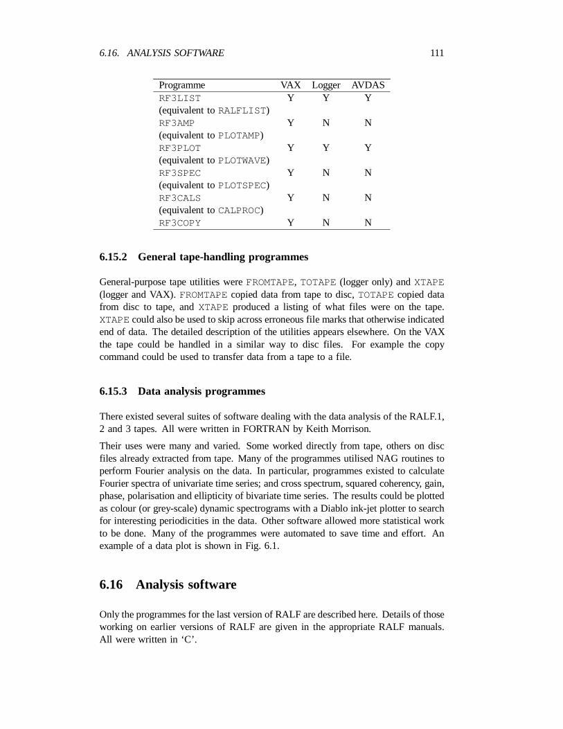
6.16. ANALYSIS SOFTWARE 111
Programme VAX Logger AVDASRF3LIST Y Y Y(equivalent toRALFLIST )RF3AMP Y N N(equivalent toPLOTAMP)RF3PLOT Y Y Y(equivalent toPLOTWAVE)RF3SPEC Y N N(equivalent toPLOTSPEC)RF3CALS Y N N(equivalent toCALPROC)RF3COPY Y N N
6.15.2 General tape-handling programmes
General-purpose tape utilities wereFROMTAPE, TOTAPE(logger only) andXTAPE(logger and VAX).FROMTAPEcopied data from tape to disc,TOTAPEcopied datafrom disc to tape, andXTAPE produced a listing of what files were on the tape.XTAPEcould also be used to skip across erroneous file marks that otherwise indicatedend of data. The detailed description of the utilities appears elsewhere. On the VAXthe tape could be handled in a similar way to disc files. For example the copycommand could be used to transfer data from a tape to a file.
6.15.3 Data analysis programmes
There existed several suites of software dealing with the data analysis of the RALF.1,2 and 3 tapes. All were written in FORTRAN by Keith Morrison.
Their uses were many and varied. Some worked directly from tape, others on discfiles already extracted from tape. Many of the programmes utilised NAG routines toperform Fourier analysis on the data. In particular, programmes existed to calculateFourier spectra of univariate time series; and cross spectrum, squared coherency, gain,phase, polarisation and ellipticity of bivariate time series. The results could be plottedas colour (or grey-scale) dynamic spectrograms with a Diablo ink-jet plotter to searchfor interesting periodicities in the data. Other software allowed more statistical workto be done. Many of the programmes were automated to save time and effort. Anexample of a data plot is shown in Fig. 6.1.
6.16 Analysis software
Only the programmes for the last version of RALF are described here. Details of thoseworking on earlier versions of RALF are given in the appropriate RALF manuals.All were written in ‘C’.
112 CHAPTER 6. RALF DATA
6.16.1 RF3LIST
This programme provides a listing of the information in the RALF data files. Theformat of the listing may be varied considerably by use of command line options. Thebasic output consists of one line for each data file giving details of the file number,the date and time of the first data record in the file, the type and the number of datarecords. Any of the following options may appear on the command line.
RECS=n Print details of the firstn data records in each file.
INFO=n Print details of the firstn information records in each file. Default isALL.
CHAN=nPrint data from channel numbern.
NUMB=nPrint data from n channels (e.g.CHAN=3 NUMB=2would print data fromchannels 3 and 4).
DATA=n Print the firstn numbers from the selected channels of each data recordthat is to be printed.
FILES=n The programme will stop aftern files have been processed.
LEN=n Sets the record length of the output device ton.
The default options areRECS=0, INFO=’ALL’ , DATA=0, CHAN=0, NUMB=1,FILES= ’ALL’ and LEN=80 (N.B. the value’ALL’ cannot be entered as suchon the command line — use any large number). The programme can process dataeither directly from the mag tape or from disc files. In the latter case it will onlyprocess one file at a time and so theFILES option is irrelevant.
$ RF3LIST [options]
Output is normally sent to the terminal but may be redirected to a file by assign-ing SYS$OUTPUT. It requires the following files for compilation:RALFLIST.C ,RALF_DAT.H, RALFTP.OBJ, TAPEI.OBJ andUTIL.OBJ .
6.16.2 RF3AMP
This programme produces a plot of the maximum amplitude or correlation levels. Theplot may be produced on a Tally printer or the DEC LA34 printer if this is connectedto the VAX. About 6 hours of data will fit onto 1 page of output. The options maybe any combination of the following.
CHAN=nTo plot channeln.
NUMB=nTo plot n channels (e.g.CHAN=6 NUMB=9will plot channels 6 to 15).
6.16. ANALYSIS SOFTWARE 113
FILES=n Stop after n files.
Defaults areCHAN=0, NUMB=6, FILES=’ALL’ . Channels 0 to 5 refer to the signalamplitude data, while channels 6 to 15 refer to the maximum cross-correlations.
$ RF3AMP [options]
Output will be written to the filePLOTOUT. This may be assigned to a file of adifferent name if required. To plot the file on a Tally printer use the command:
$ PRINT/PASSALL PLOTOUT.
If the programme has been linked for plotting on an LA34 the printer should beconnected to a terminal line and the TYPE command used to send the file to theprinter. The plot will take about 12 minutes for each day’s data. On the VAX itrequires the following files for compiling and linking:RF3AMP.C, TALLYSEQ.OBJ,RALFTP.OBJ, TAPEI.OBJ , UTIL.OBJ . TALLYSEQmay be replaced bySEQPLOTfor Epson MX-82 orLA34SEQfor DEC LA34.
$ CC RF3AMP.C$ DEFINE LNK$LIBRARY SYS$LIBRARY:VAXCRTL$ LINK RF3AMP,TALLYSEQ,RALFTP,TAPEI,UTIL
For LA34 printer output the link command would be:
$ LINK RF3AMP,LA34SEQ,RALFTP,TAPEI,UTIL
6.16.3 RF3PLOT
This programme produces a chart of the data. On the VAX the command would be.
$ RF3PLOT [options]
Any combination of the following options may be used.
FILES=n to stop aftern files have been processed (default isall ).
SKIP=n to skipn data records before starting to plot.
PLOT=n to plot n data records (default isall ).
114 CHAPTER 6. RALF DATA
6.16.4 RF3SPEC
This programme produces a dot matrix spectrogram of one channel of the high speedVLF or ULF data. Output is produced on the Tally printer. Approximately 30minutes of data will fit on one page (with defaultRANGEand REDUNparameters).The programme is run in a similar way toRF3AMP. Any combination of the followingoptions may be used.
CHAN=nTo process channeln.
FILES=n To stop aftern files.
OFFSET=n To apply an offset to the spectrogram output. The grey-scale plottingroutine attempts to show 16 different levels of grey. If an offset ofn is appliedthen a spectral amplitude that would normally be plotted with levelm willinstead be plotted with a levelm¡ n.
SCALE=n To alter the scale relating grey level to spectral magnitude. The maximumdynamic range of the data is about 96 dB. The scale value determines thenumber of grey levels mapped to this range. This will normally be¸ 16 toensure that the full range of the plot is used.
RANGE=nTo set the frequency range of the plot.n may take the value 1, 2, 5 or10 and defaults to 10. Note that the lower ranges are achieved by crude digitalfiltering of the input. This means that there is a possibility of aliasing if a lowrange is used when higher frequency signals are present.
REDUN=nTo set the redundancy or overlap factor of the plot. Setting a high redun-dancy will stretch out the plot along the time axis to give more detail of signalswith a rapidly changing spectral content. The default isREDUN=2and valuesbetween 1 and 10 may be used.
Defaults areCHAN=0, FILES=’ALL’ , OFFSET=0, SCALE=32.
6.16.5 RF3CALS
The RF3CALSprogramme is for processing all calibrations done on the ULF partof the logger (see section 6.12). It computes power and cross-spectra on the ULFchannels for a specified block of data and indicates the amplitude and relative phaseof the signal at a specified frequency. The specifications for each signal forming partof a set of calibrations are read from a control file as the programme reads the datafrom the magnetic tape.
The data are processed in blocks of 30 seconds at a time. These contain 600 highspeed data points per channel of which the centre 512 are used. A Hanning windowis applied and then a Fast Fourier Transform used to calculate a 256-point complex
6.16. ANALYSIS SOFTWARE 115
spectrum for each channel. Power and cross-spectra are then calculated. If more thanone 30 s block is used, successive power and cross spectra are averaged. The totalpower spectrum is scanned to find the peak nearest the specified frequency and thena 3-point weighted mean taken to estimate the actual frequency of the peak. Thepowers and relative phases at this frequency are then calculated.
Control and output file formats:
Each item in the control file consists of nine integers. It is convenient to put theseall on one line so that each line is one item but this is not strictly necessary since thenumbers are read in free format. The first six numbers specify the date and time ofthe start of the data block as year, month, day, hour, minute, second. The remainingnumbers are the number of 10-s logical records in the block, the reference channelfor phase measurements, and the approximate frequency in milli-Hertz of the signalto be measured.
The output from the programme is written to an output file (if one is specified) withone line for each signal measured. The first six numbers of each line give the dateand time in the same format as the control file. Next come three real numbers givingthe amplitude of theX , Y andZ channels. This is measured in decibels relative toone volt peak at the input of the logger. These are followed by the phase referencechannel indicator and two phase measurements (in degrees).
Indicator Reference First phase Second phasevalue channel channel channel
0 X Y Z
1 Y Z X
2 Z X Y
The programme is run using the following command.
$ RF3CALS [¡control file¿] [¡output file¿] [DEBUG=n]
If the control file is omitted, control input will be read fromSYS$INPUT, and noother parameters may be specified. If the output file is omitted, output will written toSYS$OUTPUT, and theDEBUGparameter cannot be included. TheDEBUGparametermay be used to select any combination of five types of debugging information. Thisis done by adding up the values of each type required from the table below to obtaina value forn. For exampleDEBUG=31will select all debugging information.
1 Informational or error messages when abnormal conditions occur, e.g. if there areno data at the time specified in the control file.
2 Indication of peak and rms broad-band amplitudes of the data for each channel.
4 Indication of each item read from the control file.
116 CHAPTER 6. RALF DATA
8 Indication of each high-speed data record read from the mag tape giving the dateand time of that record.
16 Monitoring of the process of searching for the signal in the spectrum.
The default isDEBUG=1and it is recommended that the value of the debug parameteris always odd so that the informational and error messages are not suppressed.
There are at present several restrictions on the use of the programme which couldbe removed if necessary although at present the advantages from doing so would notjustify the work involved. The time of the data block specified in the control filemust match exactly the time of a logical record on the tape. The programme cannothave a data block that starts in the middle of a logical record. This normally meansthat the times in the control file must be a multiple of ten seconds (if the logger isoperating correctly the logical record times are always multiples of ten seconds).
The number of logical records in a data block (specified in the control file) must bea multiple of three. This should not be a problem since all calibration signals arerecorded in 30-second, 1-minute or 2-minute blocks, which are 3, 6 and 12 logicalrecords. Only one signal measurement can be made on each data block. This shouldnot be a problem at present since the calibration signal generator used can produceonly one frequency at once. The data blocks specified in the control file must bein chronological order and they must not overlap. The first and last 2.2 seconds ofeach data block are not used in the calculation of the spectrum to allow for the timetaken to change the frequency and/or amplitude from one section to the next. Thismay not be sufficient in practice so a small error will occur if the calibration signalis not stable inside these times.
The code specific toRF3CALSis in the fileRF3CALS.Cand the basic spectrum anal-ysis routines in the fileDSPEC.C. These both need the header fileDCOMPLEX.H.The .C files may be compiled using theCC command in the usual way and thefollowing commands used to link the programme.
$ DEFINE LNK$LIBRARY SYS$LIBRARY:VAXCRTL$ LINK RF3CALS,DSPEC,DATATYPE,READLREC,TAPEI,UTIL
To use the programme in the way described, a symbol must be defined to run it. Ifthis is not done theRUNcommand may be used instead but then no parameters maybe specified.
Stop codes:
The programmes output a ‘stop code’ to indicate the reason for programme termina-tion. The following codes may occur.
0 Tape file mark encountered.
6.17. DERIVED DATA SETS 117
¡1 Tape or disc read error.
¡2 Double file mark (tape) or end of disc file.
¡3 Tape file mark when the logical record is incomplete.
¡4 Tape or disc read error.
¡5 Double file mark (tape) or end of disc file when the logical record is incomplete
A successful run of a programme should terminate with a stop code of 0 or¡2. Theformer will only occur if theFILES option has been used. (Note: Due to a bug inthe ‘C’ I/O system at present, it is not possible to distinguish between ‘end of file’and ‘error’ status. Any error will therefore be taken as end of file and so stop codes¡1 and¡4 will not occur.)
6.16.6 RF3COPY
This programme is used for copying selected portions of data from a RALF.3 tape toa disc file. The syntax is as follows:
$ RF3COPY ¡output file¿ [options]
where¡output name¿ is the file the data will be written to and[options] maybe any combination of the following:
SKIP=n To skip logical records on the tape before starting to copy.
TIME=hhmmTo wait until a record recorded on or afterhhmmis reached beforestarting to copy.
COPY=nTo copy a maximum ofn files on the tape.
FILES=n To read a maximum ofn files on the tape.
The defaults areSKIP=0 TIME=0 COPY=1 FILES=1 .
6.17 Derived data sets
No information available.
118 CHAPTER 6. RALF DATA
6.18 Archiving
Originally it was intended that the data should be retained on tape at Keyworth, andnot further archived. In October 1996 the 279 tapes were brought to BAS fromKeyworth to avoid incurring storage charges. At that time there was a request for thedata to be transcribed to a more modern format, e.g. CD-ROM. This has not happened.Now that the VAXes at both Keyworth and BAS have been decommissioned, thistranscription would probably have to be done commercially at a cost (1996) of around$20 per tape, a cost which may not be justified scientifically at present.
6.19 Documentation
RALF Manual, K Yearby. Contains information on the hardware, operations, etc.
6.20 References
² Gough H., Jones D. and Yearby K.H. (1987) The ULF/VLF correlator experi-ment at Halley. Br. Antarct. Surv. Bull.75, 17–29.
² Morrison K., Engebretson M.J., Beck J.R., Johnson J.E., Arnoldy R.L., CahillL.J.Jr., Carpenter D.L. and Gallani M. (1994) A study of quasi-periodic ELF-VLF emissions at three Antarctic stations. Ann. Geophys.12, 139–146.
² Perraut S., Gendrin R., de Villedary C.et al. (1978) French mobile station forrecording: description: initial results of the conjugated campaign in associationwith GEOS-1. ESASP-135, 73–84.
Chapter 7
VLF Doppler data
7.1 Brief description
Group delay and doppler shift of the whistler-mode components of MSK VLF trans-missions.
7.2 Detailed description
The BAS VLF Doppler receiver system was developed by Neil Thomson (Universityof Otago, New Zealand). The BAS receivers were first run in the Antarctic at Faradayduring 1986. The Doppler system at Faraday comprised PDP 11-23 computers from1986–March 1993 and thereafter MAC IIci computers. The Faraday Doppler systemwas run until December 1995. The system was moved to Halley in February 1995and operates presently. A similar system, producing compatible data files, has beenrun by Neil at Dunedin since 1989.
The data are used for studying plasma densities and motions in the magnetosphere,and whistler propagation through the magnetosphere and ionosphere.
7.2.1 Data files
The Doppler data files were initially recorded on 5.25” PDP-11 RX50 format discs.The precise format of the files was changed after the first year of operation, with allfiles recorded from 1987 onwards being recorded in the newer format. These datafile formats are referred to as old-style and new-style respectively. After March 1993the PDP-11 computers were replaced by MAC IIci and the data files recorded onIBM format 3.5” floppy discs, although still in the new-style. Current file archive atHalley is to DAT.
On each of the old-style discs there were one pair of files, all of which are called
119
120 CHAPTER 7. VLF DOPPLER DATA
NAADAT.FARandNAADIR.FAR. TheNAADAT.FARfile is a binary file of length768 blocks. Data is written sequentially to this file, although it may begin anywherein the file, wrapping round from the end to the beginning if necessary. The secondfile, NAADIR.FAR, contains two numbers in binary format. These give the numberof data blocks written to the file, and the position of the last block in the file to bewritten to. Some old style discs were used to record data from two separate receiverruns. The data is all written toNAADAT.FAR. The file NAADIR.FAR only containsinformation about the location of the data from the second receiver run. It is howeverpossible to locate data from the first run, since with the Doppler receiver system, newdata are always written to disc at the position immediately after the last data to bewritten to disc — the beginning of data from the second run immediately follows theend of the data from the first run.
With new style discs, data are written sequentially to a binary file, with the earliestdata at the beginning of the file.
The Doppler data are all archived on CD-ROM. On being transferred, the old-stylefiles were converted to new-style files using the FORTRAN programmeOLDNEW.
7.3 Instrument/sensor
7.3.1 Overview
The Doppler receiver system consists of an aerial, preamplifiers, MSK signal de-modulator, and a computer (PDP-11 before March 1993, then MAC IIci) running a‘Doppler Receiver Programme’. This programme establishes the bit pattern of theMSK transmission being received, and cross correlates the direct (subionospheric)signal with the delayed and frequency shifted (whistler-mode ducted) signal. Theprocess is described fully inWhistler mode signals: spectrographic group delaysby Thomson N.R. (1981). The correlation coefficients are accumulated for what istermed an integration period before being written to disc.
7.3.2 Aerials
The aerial loops are North-South and West-East magnetic loop aerials (either smallor large loops), and a vertical electric monopole.
7.3.3 Preamplifiers
The preamplifiers are purpose-built. The magnetic signal preamplifiers have relativelyflat frequency response from 100 Hz up to 25 kHz. The MSK signals received bythe Doppler receivers are mostly at frequencies greater than 20 kHz. The lowerfrequency range is used by other instruments. These preamplifiers are referred to
7.3. INSTRUMENT/SENSOR 121
as ‘Neil-type’ to distinguish them from the earlier VLF broadband (Sheffield type)preamplifiers which do not have the extended frequency response. The electric fieldsignal preamplifier is unique to the Doppler receivers. The preamplifiers and theircircuits are described in the Doppler Receiver Preamplifiers manual. The designs ofboth magnetic and electric signal preamplifiers have been slightly modified over theduration of the Doppler experiment.
7.3.4 Demodulator
The MSK signal demodulator consists of a frequency standard, and a device todemodulate MSK transmissions — called the Doppler receiver. The receiver is tunedto a particular MSK transmission. It demodulates the transmission and presents sixsignals — HXP, HXQ, HYP, HYQ, EZP, EZQ — as outputs. Only four of thesesignals are actually used in subsequent stages of the receiver system. The originalreceiver hardware design used at Faraday in 1986 was substantially modified in 1987.The new design does the same job as the original, but in a more reliable way, andhas been in use since then. Full descriptions of the receiver hardware are given inthe Doppler receiver system hardware manuals.
7.3.5 Computer—from 1986–March 1993
The final part of the receiver system was a PDP-11 computer equipped with anADV11-C analogue to digital converter, running a ‘Doppler Receiver Programme’.The receiver programme deduces subionospheric and whistler mode bit patterns, crosscorrelates and averages them, and writes the results to disc.
ADC Units
The DEC ADV11-C installed in the PDPs is used with bipolar inputs, and has aninput voltage range of§10V.
At the ADC input there is an amplifier with a selected gain of 1, 2, 4 or 8 times.The input voltage after this amplification must be in the range§10V, so choosing again of 2 reduces the maximum voltage at the outside world to§5V etc.
The digitised value is returned in a 12-bit binary integer. This gives return valuesfrom ¡2048 to +2047.
The size of one ADC unit is the voltage corresponding to a return value of 1, andmaximum voltage range at the inputequals .
2047
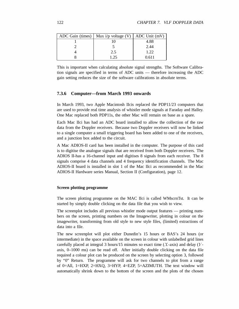
122 CHAPTER 7. VLF DOPPLER DATA
ADC Gain (times) Max i/p voltage (V) ADC Unit (mV)1 10 4.882 5 2.444 2.5 1.228 1.25 0.611
This is important when calculating absolute signal strengths. The Software Calibra-tion signals are specified in terms of ADC units — therefore increasing the ADCgain setting reduces the size of the software calibrations in absolute terms.
7.3.6 Computer—from March 1993 onwards
In March 1993, two Apple Macintosh IIcis replaced the PDP11/23 computers thatare used to provide real time analysis of whistler mode signals at Faraday and Halley.One Mac replaced both PDP11s, the other Mac will remain on base as a spare.
Each Mac IIci has had an ADC board installed to allow the collection of the rawdata from the Doppler receivers. Because two Doppler receivers will now be linkedto a single computer a small triggering board has been added to one of the receivers,and a junction box added to the circuit.
A Mac ADIOS-II card has been installed in the computer. The purpose of this cardis to digitise the analogue signals that are received from both Doppler receivers. TheADIOS II-has a 16-channel input and digitises 8 signals from each receiver. The 8signals comprise 4 data channels and 4 frequency identification channels. The MacADIOS-II board is installed in slot 1 of the Mac IIci as recommended in the MacADIOS-II Hardware series Manual, Section II (Configuration), page 12.
Screen plotting programme
The screen plotting programme on the MAC IIci is called WMscrnTst. It can bestarted by simply double clicking on the data file that you wish to view.
The screenplot includes all previous whistler mode output features — printing num-bers on the screen, printing numbers on the Imagewriter, plotting in colour on theimagewriter, transforming from old style to new style files, (limited) extractions ofdata into a file.
The new screenplot will plot either Dunedin’s 15 hours or BAS’s 24 hours (orintermediate) in the space available on the screen in colour with unlabelled grid linescarefully placed at integral 3 hours/15 minutes so exact time (X-axis) and delay (Y -axis, 0–1000 ms) can be read off. After initially double clicking on the data filerequired a colour plot can be produced on the screen by selecting option 3, followedby “0” Return. The programme will ask for two channels to plot from a rangeof 0=All, 1=HXP, 2=HXQ, 3=HYP, 4=EZP, 5=AZIMUTH. The text window willautomatically shrink down to the bottom of the screen and the plots of the chosen
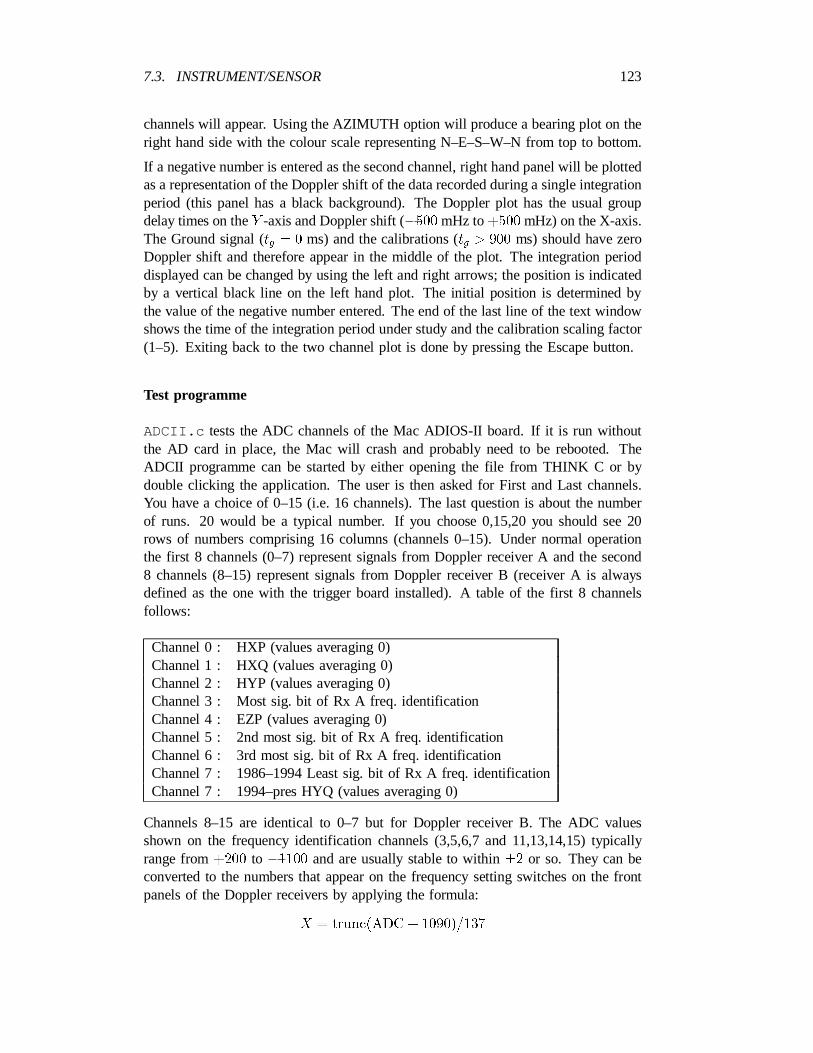
7.3. INSTRUMENT/SENSOR 123
channels will appear. Using the AZIMUTH option will produce a bearing plot on theright hand side with the colour scale representing N–E–S–W–N from top to bottom.
If a negative number is entered as the second channel, right hand panel will be plottedas a representation of the Doppler shift of the data recorded during a single integrationperiod (this panel has a black background). The Doppler plot has the usual groupdelay times on theY -axis and Doppler shift (¡500 mHz to+500 mHz) on the X-axis.The Ground signal (t = 0 ms) and the calibrations (t > 900 ms) should have zerog g
Doppler shift and therefore appear in the middle of the plot. The integration perioddisplayed can be changed by using the left and right arrows; the position is indicatedby a vertical black line on the left hand plot. The initial position is determined bythe value of the negative number entered. The end of the last line of the text windowshows the time of the integration period under study and the calibration scaling factor(1–5). Exiting back to the two channel plot is done by pressing the Escape button.
Test programme
ADCII.c tests the ADC channels of the Mac ADIOS-II board. If it is run withoutthe AD card in place, the Mac will crash and probably need to be rebooted. TheADCII programme can be started by either opening the file from THINK C or bydouble clicking the application. The user is then asked for First and Last channels.You have a choice of 0–15 (i.e. 16 channels). The last question is about the numberof runs. 20 would be a typical number. If you choose 0,15,20 you should see 20rows of numbers comprising 16 columns (channels 0–15). Under normal operationthe first 8 channels (0–7) represent signals from Doppler receiver A and the second8 channels (8–15) represent signals from Doppler receiver B (receiver A is alwaysdefined as the one with the trigger board installed). A table of the first 8 channelsfollows:
Channel 0 : HXP (values averaging 0)Channel 1 : HXQ (values averaging 0)Channel 2 : HYP (values averaging 0)Channel 3 : Most sig. bit of Rx A freq. identificationChannel 4 : EZP (values averaging 0)Channel 5 : 2nd most sig. bit of Rx A freq. identificationChannel 6 : 3rd most sig. bit of Rx A freq. identificationChannel 7 : 1986–1994 Least sig. bit of Rx A freq. identificationChannel 7 : 1994–pres HYQ (values averaging 0)
Channels 8–15 are identical to 0–7 but for Doppler receiver B. The ADC valuesshown on the frequency identification channels (3,5,6,7 and 11,13,14,15) typicallyrange from+200 to ¡1100 and are usually stable to within§2 or so. They can beconverted to the numbers that appear on the frequency setting switches on the frontpanels of the Doppler receivers by applying the formula:
X = trunc(ADC+ 1090)=137
124 CHAPTER 7. VLF DOPPLER DATA
The ADC values of the data channels (0,1,2,4 and 8,9,10,12) vary randomly withvalues depending on the strength of the signal but probably of the order of§150 orso. Each analogue input is a demodulation of the time varying MSK signal transmittedat the frequency that the receiver is set to. The ADC values should therefore havean average value of 0.
7.4 Recording method
Recordings are made by running the Doppler Receiver programme.
7.4.1 from 1986–March 1993
Several versions of the doppler receiver programme were available. They all aredescribed in the manualOverview of BAS Doppler experiment software for PDP. Todate, only two receiver programmes have been used routinely. These areNAADFandNAADFY. A description of these in included. There are certain control parametersfor the programmes. They have the following meanings:
² n = number of 25-second intervals in an integration period.
² p = total number of integration periods in a programme run.
² c = amplitude of smallest software calibration in ADC units. The other soft-ware calibrations are two and three times this amplitude.
² /G determines ADC gain/G:0 gain = 1,/G:1 gain = 2,/G:2 gain = 4,/G:3 gain = 8.
² a = automatic software calibration control reference level.
The numbers are interpreted asoctal unless followed by a decimal point.
Programme NAADF
Neil Thomson’s original programme with the minimum modifications necessary tomake it run on the Sheffield PDP and the Faraday PDPs. It is functionally identicalto the original programme described in the paper ‘Whistler Mode Signals: Spectro-graphic group delays’.
The programme is run using the following commands.
.GET NAADF
.D 1000=n
.D 1002=p
.START 1004
7.4. RECORDING METHOD 125
Programme NAADFY
This has a number of extra features added. It will decode the voltages present on someof the spare analog inputs to determine the frequency the receiver is tuned to (assumingsuitably modified receiver hardware is used). It provides a graphics display on theVT125 VDU of the HXP and HXQ signals as a function of group delay. The filenames and programme parameters (integration time, number of integration periods,and software calibration amplitude) may be set using a standard CSI (command stringinterpreter) string.
NAADFYuses only a single output file rather than separate directory and data files.A data file of the required size is allocated when the programme is started and thedata is simply written to this file sequentially. No directory file is necessary sincethe earliest data always starts at the beginning of the file. The format of each datablock (8 physical disc blocks) is similar toNAADF.
With NAADFYthe software calibrations may be adjusted automatically according tovariations in receiver sensitivity and the strength of the signals received. Automaticmode is set by specifying a (non-zero) reference level in the CSI command string(/A option). This is used as a minimum value for the upper correlation coefficientlimit. If there are whistler mode signals with a correlation coefficient greater than thereference level then these will set the upper limit. The lower correlation coefficientlimit is always 1/4 of the upper limit.
If the correlation coefficient of the largest software calibration (CAL3) is greaterthan the upper limit then the amplitude of the software calibrations will be reduced(if possible) for the following run. Likewise, if the correlation coefficient of CAL3 isbelow the lower limit the amplitude will be increased (if possible) for the followingrun.
The software calibration amplitudes are always in the ratio 1:2:3 and may vary fromminimum values of 1,2,3 to maximum values 5,10,15. The initial amplitude at thestart of the programme run may be set using the/C option and defaults to 1,2,3.
A suitable value for the reference level is twice the number of 25-second intervals in anintegration period (the/N option); all correlation coefficients seem to be proportionalto this. For a standard 15-minute integration period this makes the reference levelequal to 70. If there are no WM signals stronger than this the upper correlationcoefficient limit will be 70 and the lower limit 17.
.RUN NAADFY*¡file name¿/N:n/P:p/C:c/G:g/A:a
7.4.2 from March 1993 onwards
The Doppler programme was rewritten in C but should retain most of the featuresthat the old programme had.
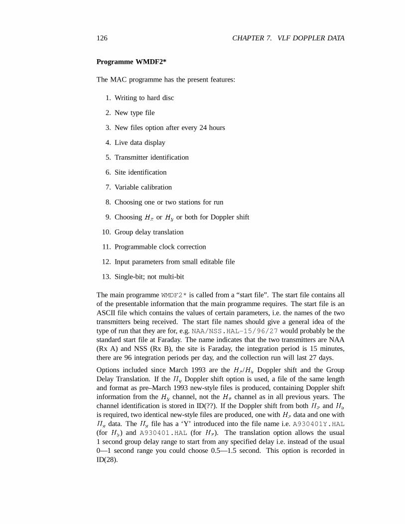
126 CHAPTER 7. VLF DOPPLER DATA
Programme WMDF2*
The MAC programme has the present features:
1. Writing to hard disc
2. New type file
3. New files option after every 24 hours
4. Live data display
5. Transmitter identification
6. Site identification
7. Variable calibration
8. Choosing one or two stations for run
9. ChoosingH or H or both for Doppler shiftx y
10. Group delay translation
11. Programmable clock correction
12. Input parameters from small editable file
13. Single-bit; not multi-bit
The main programmeWMDF2*is called from a “start file”. The start file contains allof the presentable information that the main programme requires. The start file is anASCII file which contains the values of certain parameters, i.e. the names of the twotransmitters being received. The start file names should give a general idea of thetype of run that they are for, e.g.NAA/NSS.HAL-15/96/27 would probably be thestandard start file at Faraday. The name indicates that the two transmitters are NAA(Rx A) and NSS (Rx B), the site is Faraday, the integration period is 15 minutes,there are 96 integration periods per day, and the collection run will last 27 days.
Options included since March 1993 are theH /H Doppler shift and the Groupx y
Delay Translation. If theH Doppler shift option is used, a file of the same lengthy
and format as pre–March 1993 new-style files is produced, containing Doppler shiftinformation from theH channel, not theH channel as in all previous years. They x
channel identification is stored in ID(??). If the Doppler shift from bothH andHx y
is required, two identical new-style files are produced, one withH data and one withx
H data. TheH file has a ‘Y’ introduced into the file name i.e.A930401Y.HALy y
(for H ) and A930401.HAL (for H ). The translation option allows the usualy x
1 second group delay range to start from any specified delay i.e. instead of the usual0—1 second range you could choose 0.5—1.5 second. This option is recorded inID(28).
7.5. RECORDING SITES 127
7.4.3 Operational details
The precise details of how a receiver is started have varied depending on the oper-ator and the circumstances. Possible methods range from loading the programme tomemory and modifying memory locations to set operating parameters before runningit, to running the system unattended for a month at a time. The basic operations areto ensure that the receivers are being fed a signal and are demodulating it, set thecomputer clocks accurately, and start the receiver programme to record data to a disc.
The receivers were usually run with fifteen-minute integration periods. The softwarecalibration amplitude settings and integration times are written in the VLF logbook.
7.5 Recording sites
Doppler receivers have been run at Sheffield, Faraday, Halley and Cambridge. Areceiver has also been run on board RRS Bransfield while en route between Halley andMontevideo in 1988, and two receivers were operated from Montevideo to Faradayvia Halley in 1993.
7.6 Dates/ times
The Doppler receivers have been in operation at the following times:-
Faraday: February 1986–February 1987; Feb 1988–March 1991; March 1992–December 1995
Halley: December 1987–January 1988; February 1995. . .
South Atlantic: January–February 1988; January–March 1993
Marion Island, SA: May 1996
VLF Doppler receivers have been run for test purposes at Sheffield and Cambridgeon occasions since 1985. Identical format data files have been recorded at Universityof Otago, New Zealand intermittently since 1989.
7.7 Physical media
Primary data are recorded on PDP-11 RX50 format 5.25 inch discs, stored in the VLFdata room. VLF logbooks contain start/stop times and other information relevant toDoppler data files. After March 1993, data files were written on to the MAC harddisc and later copied off on to MS-DOS format discs. Currently the data files fromthe MAC hard disc is archived to DAT at Halley and returned to Cambridge beforecopying to CD-ROM.
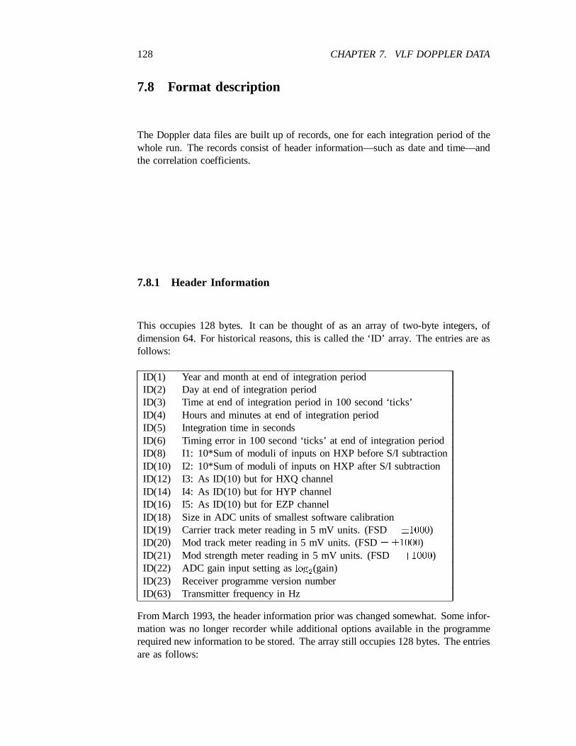
128 CHAPTER 7. VLF DOPPLER DATA
7.8 Format description
The Doppler data files are built up of records, one for each integration period of thewhole run. The records consist of header information—such as date and time—andthe correlation coefficients.
7.8.1 Header Information
This occupies 128 bytes. It can be thought of as an array of two-byte integers, ofdimension 64. For historical reasons, this is called the ‘ID’ array. The entries are asfollows:
ID(1) Year and month at end of integration periodID(2) Day at end of integration periodID(3) Time at end of integration period in 100 second ‘ticks’ID(4) Hours and minutes at end of integration periodID(5) Integration time in secondsID(6) Timing error in 100 second ‘ticks’ at end of integration periodID(8) I1: 10*Sum of moduli of inputs on HXP before S/I subtractionID(10) I2: 10*Sum of moduli of inputs on HXP after S/I subtractionID(12) I3: As ID(10) but for HXQ channelID(14) I4: As ID(10) but for HYP channelID(16) I5: As ID(10) but for EZP channelID(18) Size in ADC units of smallest software calibrationID(19) Carrier track meter reading in 5 mV units. (FSD= §1000)ID(20) Mod track meter reading in 5 mV units. (FSD= §1000)ID(21) Mod strength meter reading in 5 mV units. (FSD= +1000)ID(22) ADC gain input setting aslog (gain)2
ID(23) Receiver programme version numberID(63) Transmitter frequency in Hz
From March 1993, the header information prior was changed somewhat. Some infor-mation was no longer recorder while additional options available in the programmerequired new information to be stored. The array still occupies 128 bytes. The entriesare as follows:
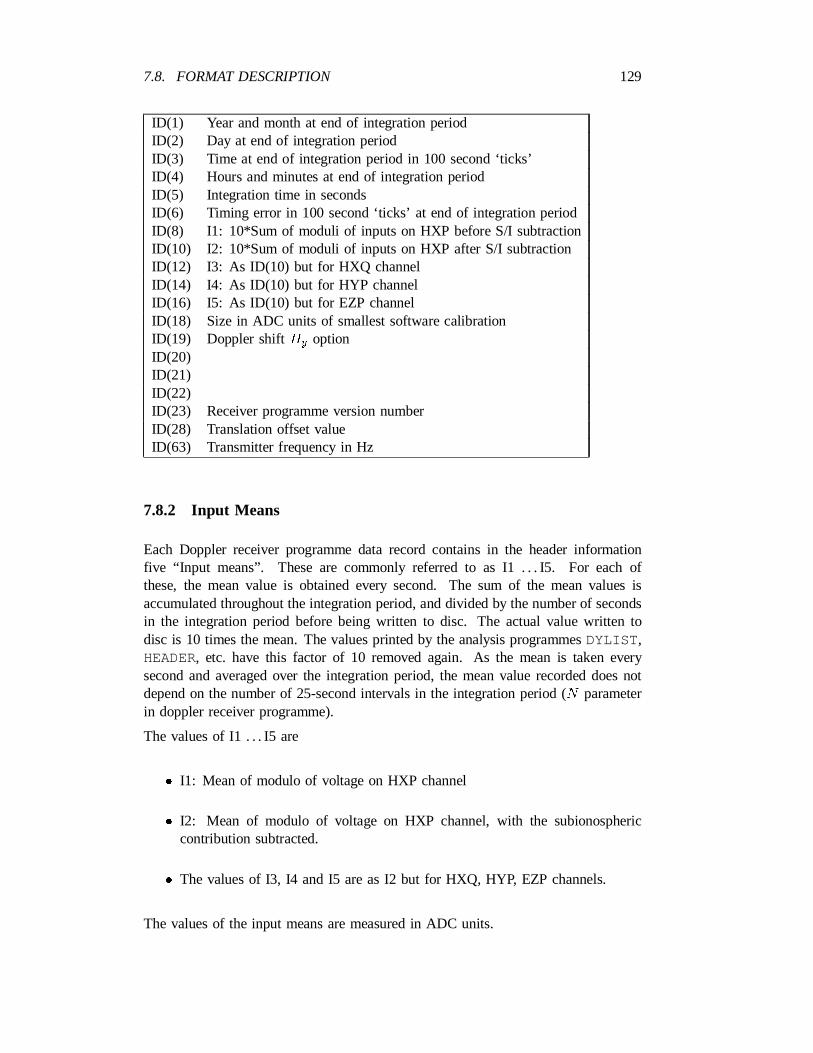
7.8. FORMAT DESCRIPTION 129
ID(1) Year and month at end of integration periodID(2) Day at end of integration periodID(3) Time at end of integration period in 100 second ‘ticks’ID(4) Hours and minutes at end of integration periodID(5) Integration time in secondsID(6) Timing error in 100 second ‘ticks’ at end of integration periodID(8) I1: 10*Sum of moduli of inputs on HXP before S/I subtractionID(10) I2: 10*Sum of moduli of inputs on HXP after S/I subtractionID(12) I3: As ID(10) but for HXQ channelID(14) I4: As ID(10) but for HYP channelID(16) I5: As ID(10) but for EZP channelID(18) Size in ADC units of smallest software calibrationID(19) Doppler shiftH optiony
ID(20)ID(21)ID(22)ID(23) Receiver programme version numberID(28) Translation offset valueID(63) Transmitter frequency in Hz
7.8.2 Input Means
Each Doppler receiver programme data record contains in the header informationfive “Input means”. These are commonly referred to as I1. . . I5. For each ofthese, the mean value is obtained every second. The sum of the mean values isaccumulated throughout the integration period, and divided by the number of secondsin the integration period before being written to disc. The actual value written todisc is 10 times the mean. The values printed by the analysis programmesDYLIST ,HEADER, etc. have this factor of 10 removed again. As the mean is taken everysecond and averaged over the integration period, the mean value recorded does notdepend on the number of 25-second intervals in the integration period (N parameterin doppler receiver programme).
The values of I1 . . . I5 are
² I1: Mean of modulo of voltage on HXP channel
² I2: Mean of modulo of voltage on HXP channel, with the subionosphericcontribution subtracted.
² The values of I3, I4 and I5 are as I2 but for HXQ, HYP, EZP channels.
The values of the input means are measured in ADC units.
130 CHAPTER 7. VLF DOPPLER DATA
7.8.3 Correlation coefficients
The correlation coefficient values are compressed before being written to the file.Although they reside in the file in a long string, the coefficients for each record mayhelpfully be regarded as constituting an array. The array has 31 columns and 200rows. The rows from 1 to 199 contain the coefficients corresponding to whistlermode group delays from¡25 ms to 965 ms in 5 ms steps. The 200th row containsthe factor by which the data was compressed for that column before being written tothe file.
Each of the 31 columns contains the correlation information at each group delay fora different ‘channel’. There are 6 channels which are sensitive to signals in a bandof width 1 Hz about the frequency to which the receiver is tuned. These channelshave sufficient bandwidth for most whistler mode signals to show up in them. Theyare used to find group delay and arrival azimuth of the signals.
They are given the following names:
HXP North South magnetic loop, in phase, unsigned
HXQ North South magnetic loop, in quadrature, unsigned
HYP West East magnetic loop, in phase, unsigned
EZP Vertical electric monopole, unsigned
HXE North South magnetic loop, in phase, with sign information from EZP
HYE West East magnetic loop, in phase, with sign information from EZP
(The labels phase and quadrature are arbitrarily assigned to the channels — and arederived from the way the MSK signals are demodulated.)
The remaining 25 channels are called the doppler channels. They are narrow band-width channels covering the frequency range§480 mHz from the frequency to whichthe receiver is tuned. The bandwidth of each channel is 40 mHz. The centre frequen-cies of the different channels are 40 mHz apart, evenly spaced around the frequency towhich the receiver is tuned. These channels contain information about the frequencyshift of the whistler mode signals.
An internally generated calibration signal (the software calibration) is added to thecorrelations to provide a signal of known size. The software calibration signals of
±zero doppler shift and¡45 arrival azimuth are added at group delays of 915 ms,935 ms and 955 ms in size ratio of 1:2:3. The calibration signal sizes are specifiedin ‘ADC units’.
7.9. SIZE OF DATA STRUCTURES 131
7.9 Size of data structures
Data for one integration period occupies 8 blocks of space. One PDP block is 512bytes, so one integration period occupies 4096 bytes, and one 24-hour long file atfifteen minute integration period occupies 393,216 bytes.
7.10 Validation
Data files may be checked for validity principally by ensuring that the header entriesfor each data record (integration period) are consistent and sensible. The headerentries may be extracted from a data file with the analysis programmeHEADER.Check the VLF logbooks to see if anything has happened to compromise the inputsignal quality. Examine a summary colour plot of the data file to see if it ‘looksright’.
7.11 Anomalous or suspect data
² In 1988 a reconfigured version of the Doppler receiver hardware was run witha cut down version of the Doppler receiver programme,RAWSAM, to recordthe demodulated signal voltages at the receiver hardware outputs, as quickly aspossible. The intention was to see if dispersion information could be obtainedfrom the upper and lower (mark and space) frequencies of a single MSK trans-mission. The files are namedRAWnnn.FAR, wherennn is a serial number.
² All the Doppler data recorded at Faraday in 1986 are subject to large clockerrors — of up to 10 minutes in 24 hours. This was because the PDP-11 clockswere then driven from the nominally 50 Hz mains. The base mains frequencytended to fluctuate, giving large clock errors. These are noted in the VLFlogbook for this period.
² At Faraday in 1986, the receiver hardware that was tuned to NAA was set up±with an unnecessary 180 of phase shift on the electric field signal. The NSS
electric field input, and the updated 1987 design receivers do not have thisextra phase shift.
² From 12 September 1989 to 21 September 1989 the Faraday doppler data wasrecorded without an electric field signal.
² From 21 September 1989 to 16 October 1989 the Faraday doppler data wasrecorded with an electric field signal from a temporary aerial, of questionablecharacteristics.
² The Doppler data recordings made on the Bransfield in 1987 and 1993 did nothave an electric field signal present.
132 CHAPTER 7. VLF DOPPLER DATA
² The Doppler data recordings made on the Bransfield in 1993 and 1993 did nothave an electric field signal present.
² From June 1995 Doppler data recordings at Faraday are affected by poor con-nections from preamplifier to receiver and also degrading buffer amplifier per-formance. This state remained (although variable) until December 1995.
7.12 Calibration
Deduction of absolute signal sizes from Doppler data files is not straightforward, andcan be regarded as a two stage process.
The sensitivity of the aerial/preamplifier/demodulator must be found. This was donetwice per year at Faraday when Doppler receivers were run there. The results arekept in the folder ‘Faraday OPAL and Doppler calibrations’.
Then, the relationship between correlation coefficient size and input signal size forthe doppler receiver programme must be established. Because of the details of thecorrelations, this relationship is very non-linear. The correlation coefficient size for aparticular whistler mode signal depends also on the sizes of all other signals present.
An instrument, the ‘Doppler Receiver Calibrator’, has been built to enable the re-sponse of the Doppler receiver programme to be investigated. It generates MSKsignals with simulated whistler mode and subionospheric components. The whistlermode component’s amplitude, ‘group delay’ and frequency may be adjusted withinrealistic bounds for real whistler mode signals. The calibrator has been used fromtime to time. Details are given in1st year PhD report, 1987, John Saxton, section6, andFaraday VLF report, 1989/90, section 18.
An empirical relationship has been found, which is thatµ ¶WM
log = constantCAL3
There is a different constant value for each CAL1 amplitude setting.
The constant does not vary (to first order) with other signal strengths or noise levels.The WM signal strength at the aerials may be found for live signals provided the
WMaerial/receiver system sensitivity has been measured, and the slope oflog hasCAL3
been found for the relevant software calibration amplitudes.
7.13 Naming/numbering conventions
Old-style Doppler data file pairs are all calledNAADIR.FAR and NAADAT.FAR.New-style pre-March 1993 files are namedtyynnn.sss or tyynnn.ssp where
t last letter of transmitter call sign
7.13. NAMING/NUMBERING CONVENTIONS 133
yy year
nnn serial number of data file
sss doppler receiver site
p data file part number (for files which were originally recorded to hard disc andwere too large to fit on one floppy disc without being split)
New-style post-March 1993 files are namedtyymmdd.sss or tyyTmmdd.sss ortyymmddY.sss where
t last letter of transmitter call sign
yy year
T if the group delay times have been ‘translated’
mmmonth
dd day
Y if the Doppler shift channel isH instead ofHy x
sss Doppler receiver site
The receiver sites currently used are
FAR Faraday
HAL Halley
SHF Sheffield
CAMCambridge
BRD RRS Bransfield
e.g.
A89144.FARA87122.HA2A930401.FARS93T0402.BRD
134 CHAPTER 7. VLF DOPPLER DATA
7.14 Catalogues
The primary reference concerning Doppler data is the handwritten VLF logbook.Catalogue information in machine readable form is also available. These cataloguesare created by programmeDOPLOGfrom the data files, with clock error and commentinformation entered by hand. The log files are inDOPLOGbinary format on PDP RX-50 format discs with one file for each receiver for each month, calledA89JUL.LOG,etc. Ordinary text format versions of the files covering one year, calledA89.CAT , etcare included in the relevant subdirectories of the optical discs where doppler data isarchived. A catalogue of file info has been made of all of the Doppler files archivedon the Optical discs. Information given includes filename, start and end times, andtransmitter frequency.
7.15 Analysis methods
Summary colour plots of ‘uncalibrated power’ for HXQ channel are made for all thedata files recorded - to provide a quick way of viewing the contents of a data file.
Group delay, doppler shift and arrival azimuth may be found directly from the corre-lation coefficients. This information obtained for whistler mode signals travelling inthe same magnetospheric duct from transmitters of two different frequencies may becombined, and theL-shell of the duct may be deduced.
Variation inL-shell, and whistler mode signal group and phase time may be used todeduce duct drifts, and particle fluxes into and out of ducts.
Details of analysis are given in PhD theses and first year reports by Mark Clilverdand John Saxton.
7.16 Analysis software
Analysis software for the VLF Doppler data exists for the PDP-11, VAX, MAC, andPC. In this manual we will concentrate on the PC programmes. The programmeswere written and modified by a variety of authors including Neil Thomson, JohnRobertson, John Saxton, Keith Yearby, and Mark Clilverd.
7.16.1 Fundamental routines
There are two routines which are necessary in all programmes which access thecorrelation coefficient information.
² UNPACK— converts a compressed array of 128 bytes into an unpacked arrayof 200 correlation coefficients.
7.16. ANALYSIS SOFTWARE 135
² IXPLOG — removes the quasi-logarithmic compression from unpacked coeffi-cients, to give linear (within the terms of reference of the receiver programme)correlation coefficients.
7.16.2 Overview
PC-DPLOT produces colour plots of doppler data files.
DOPINT This interactive programme displays a Doppler data file on a graphicsdevice, and allows points to be logged selectively,under the control of a cursor.When points are logged, group delay, doppler shift and arrival azimuth of thewhistler mode signals may be calculated.
DOPSCANAutomatically scans a whole data file for correlation coefficient peaks.When a peak is found, group delay, doppler shift and arrival azimuth of thewhistler mode signal is calculated and written to a file.
DOPCATProduces a catalogue listing of Doppler files in a directory.
DYLIST Prints all correlation coefficient and header values for a Doppler data file.
Other programmes Numerous other programmes exist for processing Doppler data.These are fully documented in the manualsOverview of BAS Doppler exper-iment software for PDP, 1 October 1990and PC Doppler Software Manual,March 6, 1991.
7.16.3 PC-DPLOT
This programme produces colour plots of Doppler data files (see examples Figs. 7.1,7.2 and 7.3).
¿PC-DPLOT ¡doppler file¿ –¡plot file¿ — *" [¡options¿]
If a <plot file > is named, the plot is written in ‘AV-GRAF’ format to that file(see Appendix E for details on how to plot these files). If* is entered, the plot ismade on the PC screen, and stays until ENTER is typed.
The<options > are
CHAN=nChannel to be plotted — HXP=1, HXQ=2, HYP=3, EZP=4, Azimuth=5,Doppler=6. The default isn = 1.
SCALE=n The plot coefficients are multiplied byn=10. The default is 10.
ECON=nIf n is non-zero, a modified rainbow palette is used which leaves most ofthe plot blank, instead of making the background blue. The default isn = 1.
136 CHAPTER 7. VLF DOPPLER DATA
WIDTH=n The plot width may be changed. The minimum value (n = 1) gives aplot half the width of that produced byDPLOT(the PDP-11 version of thisprogramme). This saves paper and ink, but gives a different appearance to theplots. The default is 2, and the maximum value is 10.
The plots are the same as those created with the PDP-11 FORTRAN programmeDPLOTwritten by John Saxton, except that a bar at the top of the plot indicates thesoftware calibration settings by its thickness.
It is usual to make routine colour plots of Doppler data files of uncalibrated power,HXQ. That is, theCHAN=2option. Plots will usually be made on the HP PaintJetprinter, using theECON=1(default) option. A batch fileDPLOT.BAT is availableto do this.
The programme is built from the source filesPC-DPLOT.C, AV-GRAF.C andAV-GRAF.H. TheMAKEdescription file to control the compilation isPC-DPLOT.M.
7.16.4 DOPINT
Plots doppler data file to the PC screen. Group delay, doppler shift and arrivalazimuth of selected whistler mode signals may be found and written to a file.
Syntax
¿DOPINT ¡filename¿ [¡options¿]
<filename > is the name of the doppler data file.
Options
<options > may be
CHAN=nSelects the data channel to be plotted to the screen. The peak findingfunctions process all channels, irrespective of theCHANoption.
n may have values 1 to 6, with the following meanings:
1. HXP
2. HXQ
3. HYP
4. EZP
5. Azimuth
6. Doppler shift
7.16. ANALYSIS SOFTWARE 137
The default forCHANis 1.
SCALE=n Scales the correlation coefficient values by a factorn=10 before plottingthem. The default value forn is 10.
ECON=nIf n is non-zero, the colours corresponding to the lowest two levels of plotsof channels 1 to 4 are changed from shades of blue to black and grey.
OFF[SET]=n Starts the plotting and processing at an offset ofn integration periodsfrom the beginning of the data file.
The peak-finding and azimuth routines are functionally similar to those developedfor the PDP-11 Doppler processing programmes, with minor modifications to correctbugs.
The command names and the way they are specified differs from the PDP interactiveprogrammes.
The Plot
The plot is of correlation coefficient size, arrival azimuth or Doppler shift of whistlermode signals, depending on the channel selected. The correlation coefficient sizesdisplayable range from 0 to greater than or equal to 90. The Doppler shifts displayablerange from¡500 mHz to+500 mHz, with 0 mHz being the centre colour of thepalette. The arrival azimuths are from 0 to 359 degrees, with the azimuths progressingwith increasing colour level in the sequence South-¿West-¿North-¿East. The axes aregroup delay from 0 ms to 965 ms vertically, and integration period number (whichcorresponds to time) from 0 to a maximum of 95 horizontally. If data files containingmore than 96 integration periods from the specified starting offset are processed withDOPINT, only the first 96 of these are plotted and may be processed. The rest areignored.
Cursor
A cursor may be moved over the plot to select the whistler-mode signals to beprocessed. Movement by one step is by the arrow keys, and by larger steps is byHome, End, PgUp and PgDn keys. One cursor step corresponds to one integrationperiod horizontally, and 5 ms group delay vertically.
Commands
Commands are given at theDOP¿prompt. Command entry is terminated with theENTER key. The command interpreter only requires sufficient characters to be en-tered to uniquely specify the command to be executed, or the parameter to be set. Inmost cases only the first character of a command need be given.
138 CHAPTER 7. VLF DOPPLER DATA
The commands areHELP, DEFAULT, QUIT, STATUS, SET, OPENandPEAK.
DEFAULTDoes nothing.
HELP Lists all the available commands.
QUIT Prompts for confirmation, then exits the programme.
STATUS Displays status information consisting of
² Data file name,
² Date of cursor position in formatyymmdd,
² Transmitter frequency in Hz,
² Amplitude of software calibration 1,
² Integration time of data file, in minutes,
² Time and group delay of the cursor position.
SET Sets parameters controlling programme operation. The command syntax is
DOP¿ SET [¡parameter¿ ¡value¿]
If no <parameter > or <value > is given, the current values of all theparameters are displayed.The parameters which may be set areEMIN, HMIN,TGWIDTH, SITE , TX andMARKER.
EMIN and HMIN are the threshold values below which correlation coefficientsare regarded as noise, for theE-field andH-field channels respectively.
TGWIDTHis the range int over which the ‘centre of gravity’ group delayg
is found, weighted according to the correlation coefficients at each groupdelay.
SITE is a two-character string giving the receiver site. This is set automati-cally from the data file name extension if it is one which is recognised.
TX is the last letter of the transmitter call sign. This is set automatically if thetransmitter frequency is recognised. It defaults to* otherwise.
MARKER: if this is non-zero, a mark is left on the plot each time a point islogged using thePEAKcommand. The default value is non-zero.
OPENOpens and closes logging the file. The command syntax is
DOP¿ OPEN [¡filename¿]
If no<filename > is given, any currently open file is closed. If a<filename >
is given, any currently open file is closed, and the new file is opened for ap-pend. When a file is opened, the Site, Transmitter, Data file name, Transmitterfrequency, E and H thresholds, TG-width parameter, and column headings arewritten to it.

7.16. ANALYSIS SOFTWARE 139
PEAK Processes data at the group delay and integration period of the cursor. TheHXP, HXQ and HYP channels are scanned for peaks, and for each channel, the‘centre of gravity’ group delay of the peak (if found) is calculated, accordingto the TGWIDTHparameter. The values for each channel are averaged —giving a mean group delay. The doppler channel(s) with the largest coefficientvalue(s) are found. A ‘centre of gravity’ Doppler shift is computed. This uses5 channels centred on the peak, if the peak is more than one channel from eitheredge of the doppler channels. If the peak is one channel from either edge ofthe doppler channels, 3 channels centred on the peak are used. If the peakincludes a channel at the edge of the doppler channels, the average dopplerchannel of all those (if there are several) is found. This gives the Doppler shiftof the whistler mode signals. Signal azimuths are calculated: The values ofthe 955 ms software calibration signals in each channel are used to scale thecorrelation coefficients of the whistler mode signals, if the software calibrationsare above theEMIN andHMIN thresholds. The average bearing is calculated.The values of the correlation coefficients in the non-doppler channels, and thet , Doppler shift and azimuth values are displayed on the screen. If a loggingg
file is open, the option is given to write the results to this.
Source files
The programme is written in C, and compiles with Microsoft C compilers V5.1 andV6.0.
The source code is held in a number of source files. These are
DOPINT.H Constant definitions, data structure definitions
DOPINT.C Main programme, initialisation
DOPIMAG.C Plotting functions, cursor graphics functions
DOPCONV.CFunctionsIXPLOG andUNPACK
DOPCUR.CCursor movement and keyboard scanning functions
DOPCMD.CProgramme command functions
DOPPKS.CFunctions for thePEAKcommand
The file DOPINT.M contains the instructions necessary to compile the programme.
7.16.5 DOPSCAN
This programme scans Doppler data files for correlation coefficient peaks and doespeak-finding on any peaks that are above a threshold value.
140 CHAPTER 7. VLF DOPPLER DATA
Syntax
¿DOPSCAN
Programme DOPSCAN
J S Robertson, October 19, 1990
Scans Doppler Data file looking for peaks.Records containing group delay, doppler shift, etcare written to the output file specified.
Enter Doppler data file name:¡filename¿
Enter 0 for full processing (including doppler channels)Enter 1 for quick processing (group delay only)¡number¿
Description
If quick processing is selected, only HXP, HXQ, HYP channels are scanned forpeaks. This means that no doppler shift information is available for any whistlermode signals found.
The group-delay range scanned for peaks is from 200 ms to 870 ms. The correlationcoefficient thresholds used to determine whether a peak is found are written into thecode, in subroutineINICOM (and are currently 15).
No adjustment of bearings is made for pre-1987 Faraday data files, with the resultthat the bearing information found for NAA files will be incorrect.
The basis of a programme to read the files created byDOPSCANhas been written.This, calledSCANPROC, at present just reads the values from the files, and doesnothing with them. The source has been commented to indicate what the variablesare and how to extend the programme.
Source files
The source code is in the filesDOPSCAN.FORand SCANPKS.FOR. The makedescription file for this programme isDOPSCAN.M.
7.16.6 DOPCAT
This programme produces a catalogue listing of the Doppler files in a directory.
7.16. ANALYSIS SOFTWARE 141
DOPCAT ¡pathname¿ [¡options¿]
The<pathname > may include the wildcards* and?. If a drive is specified, e.g.by DOPCAT a: a full filespec such as*.* or a file name must also be given, orDOPCATdoes not find any files.
Options are:
QUICK=n If n = 1, only the first record of each data file is read. The end time andnumber of records are not displayed. The default isn = 0.
IDOUT=n If n = 0, the ‘ID’ array values which are specific to the later BAS versionsof the receiver programme are not displayed. Ifn = 1, they are displayed. Ifn = ¡1, DOPCATattempts to decide whether or not they are meaningful, andif they are they are displayed. The default isn = ¡1.
Typical full output is:
Name: A89061.FARInt per=14, ADC gain setting=2, TX freq=24050, Prog Vsn=2.02Start time=890611,0452Stop time=890611,1937Number of records=60
The same file withIDOUT=0 would give:
Name: A89061.FARInt per=14Start time=890611,0452Stop time=890611,1937Number of records=60
The same file withQUICK=1 would give:
Name: A89061.FARInt per=14, ADC gain setting=2, TX freq=24050, Prog Vsn=2.02Start time=890611,0452
Note that unlike programmeDOPLOGfor the PDP,DOPCATdoes not look at corre-lation coefficient values or estimate whistler mode group delays.
7.16.7 DYLIST
This prints all correlation coefficient and header values for doppler data file.
142 CHAPTER 7. VLF DOPPLER DATA
Syntax
¿DYLISTData file name ?¡data file¿Listing file name ?¡file, PRN or CON¿START:YR,DAY,HR,MIN?yy,ddmm,hh,mmEND: YR,DAY,HR,MIN?yy,ddmm,hh,mm
Source file
The source code is all in fileDYLIST.FOR .
7.17 Derived data sets
There are a number of derived data sets created by John Saxton and Mark Clilverdduring the course of their PhDs, held on backup discs at Cambridge. These are ingeneral undocumented, and therefore not particularly useful.
A database of East–West electric fields and of particle fluxes for quiet and moderatelydisturbed times does exist.
7.18 Archiving
Doppler data files are archived to MS-DOS format optical discs. Old-style files wereconverted to new style files and given unique names before being transferred. Thefiles are in subdirectories
X:“DOPPLER“¡site¿“¡year¿
Sites are:
FARADAYHALLEYCAMBSHEFBRAN
i.e. the whole name if 8 letters or fewer, or 4 letters or more until name is unique.
7.19. DOCUMENTATION 143
The primary discs are numbered 1400 and upwards and the backup discs are numbered1500 and upwards.
7.19 Documentation
² Faraday VLF Manual(by various authors, updated Keith Yearby, 1989). Givesa description of the basic VLF system as used at Faraday.
² Faraday Doppler Manual17.9.85 (3 volumes).
² The MSK demodulator and Preamp circuits for the Faraday Doppler Experi-ment, N.R. Thomson, 17 January 1985.
² Faraday Doppler Preamplifiers Manual.
² Faraday VLF Doppler Experiment Software Documentation and Operatingmanual, 30 September 1987.
² Doppler Receiver Hardware Manual, K.H. Yearby, November 1987.
² A Calibrator for the Faraday Doppler Receiver, K.H. Yearby, 9 November1987.
² Faraday Doppler Experiment Operating Instructions and Software Documen-tation, J Robertson, 27 September 1990.
² Overview of BAS Doppler experiment software for PDP, J. Robertson, 1 Oc-tober 1990.
² PC Doppler Software Manual, J. Robertson, March 6, 1991.
² Faraday Doppler-Mac User’s Guide, M. Clilverd, November 9, 1992.
7.20 References
7.20.1 Published
² Clilverd M.A. (1990) Phenomenology of plasmaspheric electron densities andwhistler mode ducting at mid-latitudes. Ph.D. thesis, University of Sheffield.
² Saxton J.M. (1990) Plasmaspheric electric fields and plasmasphere-ionospherecoupling fluxes. Ph.D. thesis, University of Sheffield.
² Strangeways H.J. and Thomson N.R., 24 kHz MSK Doppler receiver at Faraday,Antarctica, IERE Publication No. 68, 41–47.
² Thomson N.R. (1981) Whistler mode signals: spectrographic group delays. J.Geophys. Res.86, 4795–4802.
144 CHAPTER 7. VLF DOPPLER DATA
7.20.2 Unpublished
² Yearby K.H. (1988) Report on visit to Antarctica 1987/88 season.
² Smith A.J. (1990) Antarctic trip report, 25 April 1990.
² Clilverd M.A. (1986) Faraday 1986 VLF Report. BAS Reference F/1986/O5.
² Robertson J.S. (1988) Faraday 1988 VLF Report. BAS Reference F/1988/IV1.
² Robertson J.S. (1990) Faraday 1989/90 VLF Report. BAS Reference F/1989/IV1.
² Saxton J.M. (1987) 1st Year PhD report.
Chapter 8
OPAL/OMSK/OmniPAL data
8.1 Brief description
Phase and amplitude of VLF transmissions.
8.2 Detailed description
The BAS OPAL loggers originally logged only phase and amplitude of Omega VLFtransmissions. They were upgraded in 1990, after the first complete year of Antarcticoperation, to log both Omega and MSK (US Navy) transmissions. The system wasthen renamed OMSK. The OMSK system was decommissioned in December 1995at both Halley and Faraday. An upgraded system known as OmniPAL was installedat Halley in February 1997.
The OPAL receivers were specialised narrow band receivers designed and built by theDepartment of Physics at Otago University, New Zealand; the software was writtenpartly by Otago and partly by BAS. They were run by BAS between 1988 and 1990.
Each OPAL receiver recorded the amplitude and phase of all 5 frequencies transmittedby an Omega navigational transmission station, for each of four selected stations. Twodifferent time resolutions or formats of data file were created. High speed or format1 files contain amplitude and phase values for every Omega segment of the selectedtransmitters. For average or format 2 files, the amplitude and phase values wereaveraged over each minute before being recorded. The OPAL receivers have beenrun at Sheffield, Cambridge, Faraday and Halley and by the Otago group in NewZealand.
Each OMSK receiver records the amplitude and phase of two Omega and two MSKstations. There are four different format of files: two are similar to the OPALformats and two contain information on both the high and low frequencies in theMSK transmissions. Apart from BAS data described below, OMSK receivers havebeen run in New Zealand by the Otago University group, in Durban and Sanae by
145
146 CHAPTER 8. OPAL/OMSK/OMNIPAL DATA
the Natal University group, and in Budapest by the Eotvos University group.¨ ¨
The OmniPAL receiver at Halley monitors 6 stations (1 Omega and 5 MSKs) anduses an internal frequency standard. The time resolution can be set from 50 ms to1.25 s. OmniPAL receivers and their successors “AbsPAL” receivers (for absolutephase) have been used at many locations including Hungary, South Africa, and Japan.
The main purpose of the OPAL/OMSK/Omnipal programme is to record Trimpievents on selected transmitter to receiver paths. A secondary aim is to measure thepropagation conditions throughout the day and year.
8.3 Instrument/sensor
The VLF signal is taken from the NS and WE magnetic loops, via a preamplifier. Theamplitude and phase values are determined by the specially designed OPAL receiver,and logged to MS-DOS disc by a PC running the OPAL logger programme. TheBAS OPAL receivers no longer exist, having been upgraded to OMSK receivers.Information on the receiver hardware and the logger programme is in the folderOldOPAL and OMSK Documentation. Additional information on the logger programme isavailable in the1989/90 Faraday VLF report, BAS reference No F/1989/IV 1, section9. The source code for the Faraday OPAL logger programme is in the disc box marked“OPAL Software 2”, on disc “Faraday Software 1990, MS-DOS, Modified Loggerand Processing Programmes”, in the subdirectory LOGGER. The Halley logger sourcecode is in the disc box marked “OPAL Software 1”, on disc “OPAL 2 Old SoftwareDevelopment”. The source file names are given in the fileOPAL.M in each case.Details of the OMSK hardware and the OMSK logger programme are given in thefolder marked “OMSK Manual”. The OMSK source files for Halley and Faraday areon the discs in the boxes marked “OMSK Software”.
In the OmniPAL system the broadband signals are processed by a DSP board pluggedinto a PC. This does all the filtering and signal processing under the control of specialOmniPAL software. Copies of the latter may be found on the RSEG VLF CD-ROM.
8.4 Recording method
For OPAL, this is described in theOPAL Logger Manual, K H Yearby, Sept 1988, inthe folderOld OPAL and OMSK Documentation. For OMSK it is described in theOMSK Manual. Briefly, the logger programme (OPAL.EXE or OMSK.EXE) createsMS-DOS format files containing the amplitude and phase values detected by theOPAL or OMSK.
OmniPAL recording details may be found in the revisedHalley VLF Manualor in thedocumento:“uasd“wave“docs“omnipal.rtf . Time information came fromthe Omega signal until 30 September 1997 (see Appendix D). From 30 September1997 to 23 October 1997 the time reference on the system was simply the PC s own
8.5. RECORDING SITES 147
internal clock linked byTBASEPCto Chronos (the Halley time server, synchronised toGPS time). From 23 October 1997 OmniPAL has used an external frequency standard,a Rubidium oscillator providing an accurate 1 MHz clock. The PC’s internal clock isset viaTBASEPCat startup, and from this point on timing is derived from the 1 MHzexternal signal. This required a new version of software calledOmnipal0.exe(Version 2.1).
8.5 Recording sites
Faraday, Halley, Sheffield, Cambridge, Rothera.
8.6 Dates/ times
8.6.1 Dates
The OPALs were delivered to Sheffield, and tested there from October 1988 to De-cember 1988.
The OPAL receivers were run at Faraday from 31 March 1989 until 4 April 1990,when the receivers were converted to OMSK specification.
The OPAL receivers were run at Halley from 18 December 1988 until 15 August1990.
The OMSK receivers were run at Faraday from 2 April 1990 to 1 May 1991. Therewas then a data gap until recordings recommenced on 9 Jan 1992. The receiverswere shut down finally in December 1995.
The OMSK receivers were run at Halley from 31 July 1990 to 3 Dec 1990. Therewas then a data gap until recordings recommenced at the new Halley-5 site on 29Jan 1992. The receivers were shut down finally in November 1995.
Some OMSK recordings were made at Cambridge during the northern winter 1990–91.
OMSK recordings were made at Rothera during austral winter 1994 and 1995, aspart of an international US-UK-Brazil collaboration.
OmniPAL recordings began at Halley in February 1997 and continue to the present.
8.6.2 Times
OPAL
In general two 12-hour high speed files and two 12-hour averaged files were recordedeach day at Halley and Faraday. The 12-hour intervals were 02–14 UT and 14–02 UT
148 CHAPTER 8. OPAL/OMSK/OMNIPAL DATA
(MLT ' UT¡4.5 hrs at Faraday; UT¡3 hrs at Halley).
OMSK, 1990–91
In general two 10-hour SHL files were recorded each day at Halley and Faraday.The 10-hour intervals were 04–14 UT and 18–04 UT. Because the host computer(Amstrad) had two 360 k-byte floppy drives and no hard drive, it was not convenientto acquire 24-hour coverage.
OMSK, 1992–1995
Each day, at Halley and Faraday, two consecutive SHL files were recorded 06:30–16:30 UT and 16:30–02:30 UT, and an FHL file 02:30–06:30 UT. A similar pro-gramme was run at Sanae from 1993 onwards. This programme was been designedto have
² 24 hour coverage
² higher time resolution data at night (particularly after local midnight)
² a repeating daily pattern
² file sizes which fitted on a floppy disc, for ease of portability (one disc (360 k-bytes) could hold a 10-hour SHL file (358800 bytes) or a 4-hour FHL file(352800 bytes)).
OmniPAL, 1997–
At Halley one file is generated for each day of operation (00:00 UT–23:59 UT).The time resolution is 400 ms (equivalent to FHL) and the file size approximately4 Mb. All phase and amplitude information for the 6 transmitters under observationis incorporated in this file.
8.6.3 Transmitter selections
OPAL
Site Receiver STAT=0 STAT=1 STAT=2 STAT=3Faraday 1 ARG HAW REU HAWFaraday 2 ARG HAW DAK NORHalley 1 ARG LIB DAK HAWHalley 2 ARG LIB DAK NOR
Receiver 1 was used most of the time at both stations.
8.7. PHYSICAL MEDIA 149
OMSK
Site Receiver STAT=0 STAT=1 STAT=2 STAT=3Faraday 1 & 2 ARG HAW NAA NPMHalley 1 & 2 ARG LIB NAA NSSRothera 1 ARG LIB NAA NSS
OmniPAL
From 10 February 1997 until 23 October 1997 (after the shutdown of the OMEGAnavigation system on 30 September 1997) the Halley Omnipal receiver was set torecord the following transmitters:
Site Receiver Stat 0 Stat 1 Stat 2 Stat 3 Stat 4 Stat 5Halley 1 ARG GQD NLK NAU JXN NAA
From 23 October 1997 to the present the Halley Omnipal receiver has been set torecord the following frequencies:
Site Receiver Stat 0 Stat 1 Stat 2 Stat 3 Stat 4 Stat 5Halley 1 NPM NLK NAU JXN NAA
The N–S loop is used for all channels except NLK, for which the E–W loop is used.
8.6.4 Frequency assignments
Omega frequencies
FREQ=0 FREQ=1 FREQ=2 FREQ=3 FREQ=4f (kHz) 10.2 13.6 11.33 11.05 Unique
Omega unique frequencies
Transmitter Argentina Liberia N. Dakota LaReunion Hawaii NorwayUnique (kHz) 12.9 12.0 13.1 12.3 11.8 12.1
For more information on transmitters used, see Appendix D.
8.7 Physical media
The data files were originally recorded on MS-DOS format 5.25 inch floppy discs,formatted for 360 k-bytes. From 1992, the data were recorded temporarily on hard
150 CHAPTER 8. OPAL/OMSK/OMNIPAL DATA
disc and then transferred to transportable media for shipment to HQ (5.25” floppydiscs at Faraday; 800 M-byte optical WORM discs at Halley). OmniPAL data arecurrently written to DAT at Halley and transferred to CD-ROM at Cambridge.
8.8 Format description
8.8.1 OPAL
The OPAL logger file formats are fully defined by the “C” structures in the fileOPALFORM.H. Functions, written in “C”, to manipulate data in the various formatsexist in file OPALCONV.C. Both these files are on disc “OPAL logger and analysissource files up to August 1989” in disc box “OPAL Software 1”. A brief descriptionfollows.
The data files consist of records, each covering five minutes. The format of a recordmay be one of three types, format1, format2, and format3. With one exception (atSheffield), only format1 (high speed files) and format2 (average files) were recordedto disc.
The first 9 bytes of all the records are the same. They form the header part, containingdate and time information, and information about the OPAL receiver.
Most of the rest of each record is used to store logged amplitude and phase values.
Format1 (HS) The mean value of each amplitude and phase for each station andfrequency is compressed to 12 bit numbers and stored in12bitmeans. Thedifference between the logged value and the mean for each station/ frequency/minute/ epoch/ segment is logarithmically compressed tologdifs. The OPALreceiver gains for each station/ frequency/ minute are stored innibgains.
Format2 (AV) The value of amplitude or phase at each segment of Omega trans-mission may not be recovered from a format2 record. The differences fromthe means are not recorded as above. Instead12bitmeanscontains the meanamplitude and phase for each minute/ station/ frequency.
Format3 This contains almost the same information as a format1 record, althoughthe values are not compressed.
Records of all formats have an offsets array. The offsets are the OPAL receiverdemodulator DC offsets, which are subtracted from the logged values during conver-sion from format3 records to the other two. The values are kept in the format1 and2 records so they may be inspected as a check on the receiver.
Functions to convert between different formats are contained in fileOPALCONV.C.
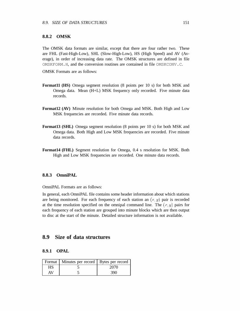
8.9. SIZE OF DATA STRUCTURES 151
8.8.2 OMSK
The OMSK data formats are similar, except that there are four rather two. Theseare FHL (Fast-High-Low), SHL (Slow-High-Low), HS (High Speed) and AV (Av-erage), in order of increasing data rate. The OMSK structures are defined in fileOMSKFORM.H, and the conversion routines are contained in fileOMSKCONV.C.
OMSK Formats are as follows:
Format11 (HS) Omega segment resolution (8 points per 10 s) for both MSK andOmega data. Mean (H+L) MSK frequency only recorded. Five minute datarecords.
Format12 (AV) Minute resolution for both Omega and MSK. Both High and LowMSK frequencies are recorded. Five minute data records.
Format13 (SHL) Omega segment resolution (8 points per 10 s) for both MSK andOmega data. Both High and Low MSK frequencies are recorded. Five minutedata records.
Format14 (FHL) Segment resolution for Omega, 0.4 s resolution for MSK. BothHigh and Low MSK frequencies are recorded. One minute data records.
8.8.3 OmniPAL
OmniPAL Formats are as follows:
In general, each OmniPAL file contains some header information about which stationsare being monitored. For each frequency of each station an(x; y) pair is recordedat the time resolution specified on the omnipal command line. The(x; y) pairs foreach frequency of each station are grouped into minute blocks which are then outputto disc at the start of the minute. Detailed structure information is not available.
8.9 Size of data structures
8.9.1 OPAL
Format Minutes per record Bytes per recordHS 5 2070AV 5 390
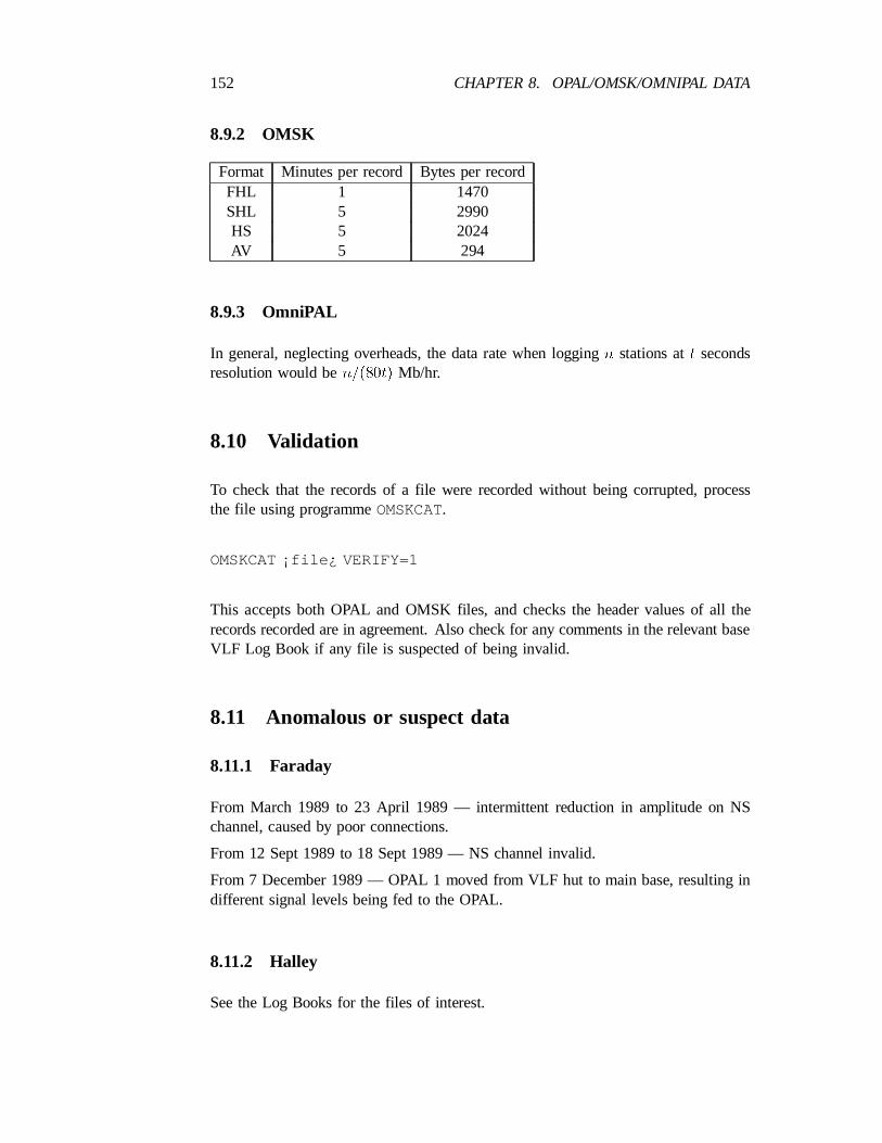
152 CHAPTER 8. OPAL/OMSK/OMNIPAL DATA
8.9.2 OMSK
Format Minutes per record Bytes per recordFHL 1 1470SHL 5 2990HS 5 2024AV 5 294
8.9.3 OmniPAL
In general, neglecting overheads, the data rate when loggingn stations att secondsresolution would ben=(80t) Mb/hr.
8.10 Validation
To check that the records of a file were recorded without being corrupted, processthe file using programmeOMSKCAT.
OMSKCAT ¡file¿ VERIFY=1
This accepts both OPAL and OMSK files, and checks the header values of all therecords recorded are in agreement. Also check for any comments in the relevant baseVLF Log Book if any file is suspected of being invalid.
8.11 Anomalous or suspect data
8.11.1 Faraday
From March 1989 to 23 April 1989 — intermittent reduction in amplitude on NSchannel, caused by poor connections.
From 12 Sept 1989 to 18 Sept 1989 — NS channel invalid.
From 7 December 1989 — OPAL 1 moved from VLF hut to main base, resulting indifferent signal levels being fed to the OPAL.
8.11.2 Halley
See the Log Books for the files of interest.
8.12. CALIBRATION 153
8.12 Calibration
A direct calibration of the OPAL or OMSK systems is not possible. The basic ideais to measure the absolute strengths of signals recorded by the instrument at a knowntime, and compare the absolute values with the values recorded at that time. Thishas been done at Faraday using a spectrum analyser, and a prototype AVDAS, and atHalley using an AVDAS. The procedure using a spectrum analyser is given in detailin the Faraday 1989/90 VLF Report(BAS reference F/1989/IV 1), page 48. Theprocedure at Halley is described in theHalley VLF Manual, Section 12.10.
8.13 Naming/numbering conventions
OPAL and OMSK files are named as follows:Osryynnn.mm[m] where:
O indicates that the file is from the OPAL/OMSK system.
s is the site identifier — F for Faraday, Z for Halley, etc.
r is the receiver number at that site — 1, 2, etc.
yy is the last two digits of the year - 89, 90, etc.
nnn is a serial number for the file.
mm[m] is the code identifying the format: either FHL, SHL, HS or AV.
OmniPAL files are named as follows:OddmmmmyA.HALwhere:
0 indicates an Omnipal file.
dd is the day of the month.
mmmmis the month.
y is the year i.e. 6 indicates 1996.
HAL is the station id i.e. HALLEY.
8.14 Catalogues
Each OPAL data file that has been recorded is detailed in the base Log Books.Machine readable catalogues consisting of the output from programmeOPALCATforeach of the files recorded also exist. These are namedOsryy.CAT .
O indicates that the file is from the OPAL system.
154 CHAPTER 8. OPAL/OMSK/OMNIPAL DATA
s is the site identifier — F for Faraday, Z for Halley, etc.
r is the receiver number at that site — 1, 2, etc.
yy is the last two digits of the year — 89, 90, etc.
CAT indicates that the file is a catalogue.
The catalogue files are held on floppy disc, and copies are on the optical disc archiveand can also be found on the corresponding CD-ROM.
Similar catalogues exist for the OMSK series files.
8.15 Analysis methods
Analysis is carried out on a PC using the software listed in the following section.
8.16 Analysis software
8.16.1 Overview
The analysis software is kept on floppy disc in the boxes “OPAL SOFTWARE 1”and “OPAL SOFTWARE 2”. The contents of these discs are listed in the folderMS-DOS disc catalogues. Full descriptions of the OPAL programmes are given in theOPAL software manual. The OMSK software is documented in theFaraday OMSKManual.
The following is a brief description of all the processing programmes currently avail-able. They are written in “C”, and run on PC. The programmes whose names beginwith OPAL are for processing OPAL files only. Those whose names begin withOMSK are for processing OMSK files, with the exception ofOMSKCAT, whichworks with both types of file. The programmes were written by Keith Yearby, KitAdams and John Robertson.
OPALCATProduces a catalogue entry for a data file, containing start/stop times, etc.Also a Verify option.
OPALVIEWDisplays 5 minutes or 1 hour of data to a PC screen.
OPALPLOTAs OPALVIEW, but also dumps the screen to an Epson-compatible dot-matrix printer.
OPALAVConverts format 1 (HS) files to format 2 (AV) files.
OPALLIST Lists amplitude and phase values for selected stations or frequencies, innumerical form.
8.16. ANALYSIS SOFTWARE 155
OPALCSVLists amplitude and phase values for selected stations or frequencies in“Comma Separated Value” numerical form suitable for loading into a spread-sheet programme.
OPALCSV1Lists amplitude and phase values for selected stations or frequencies innumerical form suitable for loading into a spreadsheet programme.
OPALSEQPlots amplitude and phase values for selected stations or frequencies onan Epson-compatible dot-matrix printer.
OPALSEQDPlots amplitude and phase values for selected stations or frequencies ona DEC LA100 compatible printer.
OPALSQFPlots amplitude and phase values for selected stations or frequencies withmaximum time resolution on an Epson-compatible dot-matrix printer.
OPALSQFDPlots amplitude and phase values for selected stations or frequencieswith maximum time resolution on a DEC LA100 compatible printer.
OPALHISS Plots hiss and spherics values on an Epson-compatible dot-matrix printer.
OPALINT Interactive programme to log amplitude and phase values to files. Intendedto be used to “scale” Trimpi events.
OPALCOPYRecovers data files from discs which have been corrupted by the loggercomputer crashing.
OPALRMSProducesOPALSEQtype plot of rms noise on amplitude and phase values.
OSPLIT Programme to split OPAL data files into smaller parts.
OPALCURSimilar toOPALINT, although with a more sophisticated way of scalingTrimpi events.
OMSKCATCatalogues and verifies OMSK files; similar toOPALCATbut works witheither OPAL or OMSK files.
OMSKLIST Lists OMSK amplitude and phase values in numerical form to the PCscreen or a file; similar toOPALLIST but for OMSK files.
OMSKVIEWPlots data files on the PC screen; similar toOPALVIEWbut for OMSKfiles. Hardcopy plots can be produced (see example Fig. 8.5).
CONVFTOSConverts an FHL data file to an SHL data file.
OMSKSEQPlots data on a dot-matrix computer (Epson compatible); similar toOPALSEQ,but for OMSK files (see examples Figs. 8.1–8.4).
OMSKCOPYFor tidying up OMSK logger files that have not been properly closeddue to power cuts or crashes; similar toOPALCOPYbut for OMSK files.
156 CHAPTER 8. OPAL/OMSK/OMNIPAL DATA
OMSKDETScans an OMSK data file for possible Trimpi events; similar toOPALDET,but for OMSK files.
OMSKSCALScales Trimpi events; similar toOPALINT but for OMSK files.
AnalyseFHL and AnalyseSHL Similar to OMSKSCALbut runs on an AppleMAC computer.
8.16.2 OPALSEQ
OPALSEQproduces chart plots of the OPAL data on a dot matrix printer. (TheSEQ part of the name stands for ’sequential plotting’; this is necessary when plottingdirectly on a dot matrix printer that does not have the random positioning capabilityof a graphics screen or pen plotter.)
The command for running this programme is:
OPALSEQ ¡filename¿ [options]
¡filename¿ is an MSDOS file name including the path if required. No wildcardsare allowed.
The options may be any combination of the following.
FORM=nThe value ofn determines whether format 1 or format 2 data is output. Ifn = 2 is selected and the file is format 1 the data will be converted. Otherwisethe format option must match the format of the file. Ifn = 1, each record isplotted as a separate frame. Ifn = 2, up to 12 hours data (144 records) areplotted on one page. The default isn = 2.
START=n Determines how many records will be skipped before starting. Default isn = 0.
NUMB=nDetermines how many records will be output. Default isn = 1.
FREQ=n or STAT=n The plot may contain either all the stations at one particularfrequency or all the frequencies for one station. These options determine whichstation or frequency is the one plotted. The default isFREQ=4which gives aplot of the unique frequencies of the four stations.
CORR=nSets a correction for phase winding caused by the frequency drift of thelocal frequency standard.n is the correction required as an integer number of
10parts in10 .
AR=n Sets the maximum amplitude range in dB’s that is to be plotted. Amplitudesoutside the range0 to n will be wrapped to within that range.A0 may alsobe specified to offset the range from zero. If not specified, the data are “auto-scaled”.
8.16. ANALYSIS SOFTWARE 157
PR=n Sets the maximum phase range in degrees that is to be plotted. Phases outsidethe range0 to n will be wrapped to within that range. Note that for sensibleresults 360 should be a multiple ofn. POmay also be specified to offset therange from zero. If not specified, the data are “auto-scaled”.
LIN=n Use linear scale for Amplitude rather than the default logarithmic (n = 0:no, n = 1: yes). In linear mode, amplitudes outside the range specified byA0andAR are clamped at the extremes of the range, rather than being wrapped.There is no effect on the phase.
Similar command syntax and options are used for other processing programmes suchasOPALLIST, OPALVIEW, OPALINT.
The following example shows how to plot all 12 hours of an averaged data file. Theplot will contain the unique frequencies for the four stations.
¿opalseq a:s288012.av numb=144
8.16.3 OMSKCAT
This is used to produce a catalogue listing of OMSK or OPAL files in a directory,and supersedes programmeOPALCAT. It accepts either old OPAL type files or newOMSK type. The four OMSK formats are fully supported.
Information is all written to ”stdout” and is therefore available for redirection. Detailswritten include: file name, format number, recording site, stations recorded, start timeand end time.
The command for running this programme is:
OMSKCAT ¡filename¿ [¡options¿]
¡filename¿ is an MSDOS filename including the path if required, and it may alsocontain the standard wildcards* and?. Any wildcards required must be explicitlyspecified—it is not sufficient to typeOMSKCAT a:.
¡options¿ may beVER[IFY]=n , OPAL[COMP]=n andERR=n, wheren is in-teger. An option is selected when a non-zeron is specified.
The effects of the options are:
VERIFY The checksums of every record in the file are tested and the contents ofeach record header are checked against the first one for consistency. Any errorsare reported.
OPAL[COMP] Selects full compatibility withOPALCAToutput. This option onlyhas any effect when old OPAL files are being catalogued, and suppresses the re-ceiver number and format name information which was not listed byOPALCAT.
158 CHAPTER 8. OPAL/OMSK/OMNIPAL DATA
ERR Stops the cataloguing of a file oncen records have been found which are inerror. This only has any effect if theVERIFY option is selected too.
Default options areVERIFY=0, OPALCOMP=0, ERR=10.
The following is an example of the output fromOMSKCAT:
Name: a:OF290013.SHLFormat no.: 13 (SHL), recording site FARADAY, OMSK No 2Stations recorded: ARG, HAW, NAA, NPMStart time: 05:59:54 06/04/90End time: 15:59:54 06/04/90Number of records: 121, record size: 2990
8.16.4 OMSKLIST
OMSKLIST is a programme for listing OMSK data on the PC screen (or optionallyinto files using the DOS redirection operator¿).
The programme is run using the command:
OMSKLIST file-name [options]
wherefile-name is the name of the file containing the data, andoptions maybe any of the following.
START=hhmmStart processing from timehhmm.
NUMB=nProcessn minutes data.
FORMAT=nProcess in formatn. n = 1: high res;n = 2: averaged.
DIF=n For MSK, list H+L and H¡L (n = 1) or H and L (n = 0).
STAT=n Include station no.n, all frequencies.
The defaults areSTART=0 (i.e. from the beginning of the file),FORM=1, DIF=1 ,STAT=0.
The listing will generally contain all stations of the type (Omega or MSK) of the onespecified; that is, in a standard file where stations 0, 1 are Omega and stations 2,3 are MSK, selectingSTAT=0 would list all Omega stations and selectingSTAT=3would list all MSK stations. The only exception to this is for the averaged Omegadata where only the specified station is listed. The output format is designed sothat for the standard data files the listing will fit on a standard 80-column screen orprinter.
The following is an example of the output fromOMSKLIST:
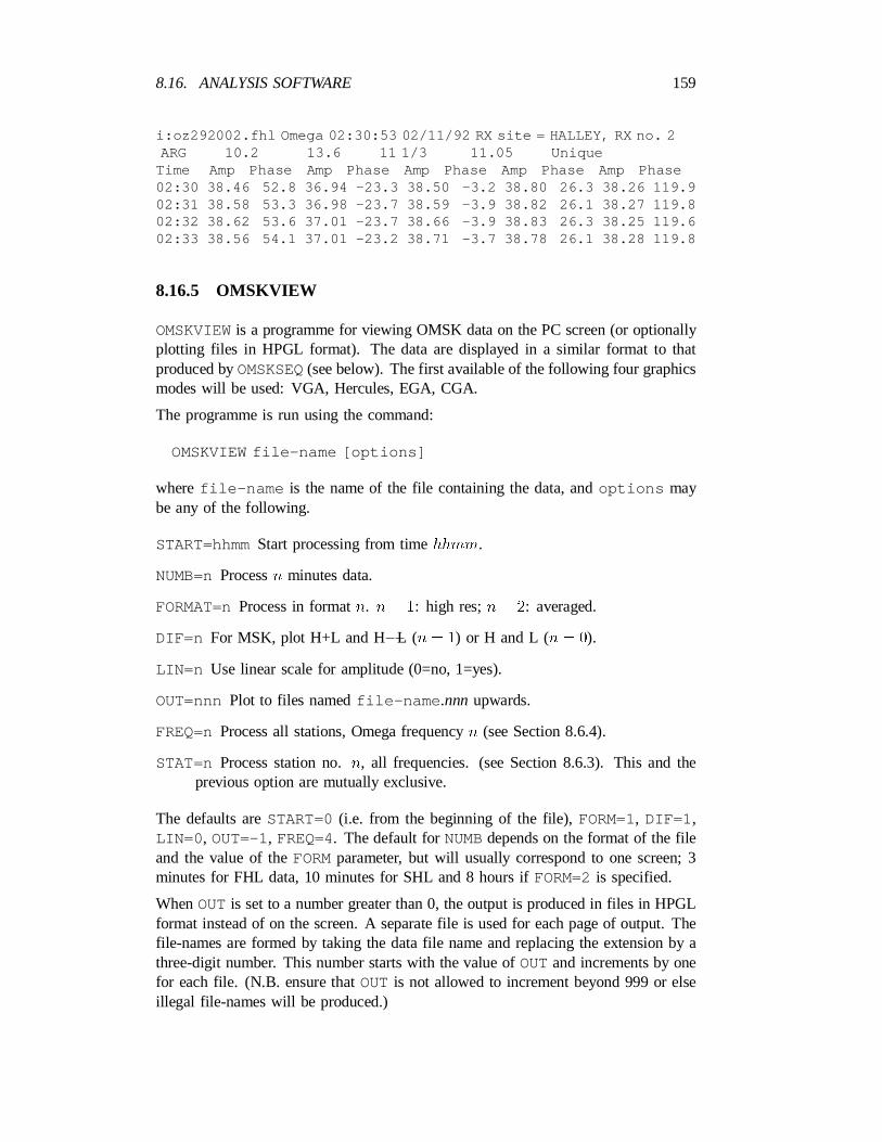
8.16. ANALYSIS SOFTWARE 159
i:oz292002.fhl Omega 02:30:53 02/11/92 RX site = HALLEY, RX no. 2ARG 10.2 13.6 11 1/3 11.05 Unique
Time Amp Phase Amp Phase Amp Phase Amp Phase Amp Phase02:30 38.46 52.8 36.94 -23.3 38.50 -3.2 38.80 26.3 38.26 119.902:31 38.58 53.3 36.98 -23.7 38.59 -3.9 38.82 26.1 38.27 119.802:32 38.62 53.6 37.01 -23.7 38.66 -3.9 38.83 26.3 38.25 119.602:33 38.56 54.1 37.01 -23.2 38.71 -3.7 38.78 26.1 38.28 119.8
8.16.5 OMSKVIEW
OMSKVIEWis a programme for viewing OMSK data on the PC screen (or optionallyplotting files in HPGL format). The data are displayed in a similar format to thatproduced byOMSKSEQ(see below). The first available of the following four graphicsmodes will be used: VGA, Hercules, EGA, CGA.
The programme is run using the command:
OMSKVIEW file-name [options]
wherefile-name is the name of the file containing the data, andoptions maybe any of the following.
START=hhmmStart processing from timehhmm.
NUMB=nProcessn minutes data.
FORMAT=nProcess in formatn. n = 1: high res;n = 2: averaged.
DIF=n For MSK, plot H+L and H¡L (n = 1) or H and L (n = 0).
LIN=n Use linear scale for amplitude (0=no, 1=yes).
OUT=nnn Plot to files namedfile-name .nnn upwards.
FREQ=n Process all stations, Omega frequencyn (see Section 8.6.4).
STAT=n Process station no.n, all frequencies. (see Section 8.6.3). This and theprevious option are mutually exclusive.
The defaults areSTART=0 (i.e. from the beginning of the file),FORM=1, DIF=1 ,LIN=0 , OUT=-1, FREQ=4. The default forNUMBdepends on the format of the fileand the value of theFORMparameter, but will usually correspond to one screen; 3minutes for FHL data, 10 minutes for SHL and 8 hours ifFORM=2is specified.
WhenOUTis set to a number greater than 0, the output is produced in files in HPGLformat instead of on the screen. A separate file is used for each page of output. Thefile-names are formed by taking the data file name and replacing the extension by athree-digit number. This number starts with the value ofOUTand increments by onefor each file. (N.B. ensure thatOUTis not allowed to increment beyond 999 or elseillegal file-names will be produced.)
160 CHAPTER 8. OPAL/OMSK/OMNIPAL DATA
8.16.6 CONVFTOS
CONVFTOSconverts an FHL data file to an SHL data file. It is run using thecommand:
CONVFTOS input_file output_file
8.16.7 OMSKSEQ
This is data plotting programme which sends output to an Epson compatible dot matrixprinter. It uses a generalised table-driven system for handling various data formatsincluding OPAL HS and AV files. The programme is run using the command:
OMSKSEQ ¡filename¿ [options]
The options are:
FORM=nIf n = 1, the data are plotted in the highest time resolution possible for themode of the data. Ifn = 2, the data are integrated into minute averages. AVfiles automatically useFORM=2.
START=n Starts plotting after skippingn minutes of data (but always starts on arecord boundary). Since the logging modes generate both 1 minute (FHL) and5 minute data records, minutes were chosen as the units for this option.
NUMB=nPlotsNUMBminutes of data (rounded to an integral number of data records).
FREQ=n or STAT=n As for OMSKVIEW.
LIN=n If n = 1, the amplitude scale is linear, otherwise it’s dB.
INF=n If n = 1, the means and standard deviation of the data are printed out. Thisis mainly for testing the noise performance of the various MSK demodulationcodes.
DIF=n If n = 1 (the default), it plots the means MSK frequency (H+L) and thedifference between the high and low frequencies (H¡L). If n = 0, it plots Hand L separately.
Each graph is separately scaled according to the range of the data, and the ranges areadjusted to 1, 2, or 5 times a power of 10.
8.16.8 OMSKCOPY
This programme is for tidying up OMSK logger files that have not been properlyclosed due to power cuts or crashes. It will copy part or all of one or several OMSKlogger files into a single new file. The syntax is as follows (similar toVLXCOPY;see Chapter 9):
8.16. ANALYSIS SOFTWARE 161
OMSKCOPY file1 [/s=skip] [/n=count] file2 .... output-file
The output file is always the last parameter on the line; the programme opens thisfirst so that it has somewhere to write the data from the input files. The outputfile must not already exist. The only limit on the number of input files is the DOScommand line length.
The skip parameter is the number of data records that will be skipped before startingto copy data to the output file. It defaults to zero. Thecount parameter specifiesthe maximum number of data records that will be copied to the output file. It defaultsto the whole file (actually 32767). The skip and number parameters refer to the fileimmediately on their left. These parameters must be specified separately for eachinput file if required.
OMSKCOPYwill only copy files of one particular format (i.e. SHL, FHL etc.); thisis determined by the format of the first input file. It does not have the formatconversion feature ofVLXCOPY. If records of a different format are encountered inthe first or subsequent input files this is taken as being the end of the valid data andthe programme will move on to the next file (if there is one). The skip parametermay be used to pass over bad records in a file; the format is checked only whencopying, not when skipping.
8.16.9 OMSKDET
The OMSKDETTrimpi detection programme scans the MSK channels of FHL, SHLformat files (it will probably also work on HS format files) and cross-correlates thevalues found with an idealised Trimpi event shape. Whenever the correlation coeffi-cient exceeds a threshold, the programme simply outputs the Trimpi event occurrencetime and significance level to “stdout” and to a file in the current directory with thesame name as the input file but with extension.tim . This can be read by the Trimpianalysis programmes (OMSKSCALon a PC, orAnalyseFHL or AnalyseSHL ona Macintosh) in order to locate previously detected Trimpi events for scaling.
Optionally, if the output of.DET files is enabled by theDET=1command line option,the programme will write to disc a.DET file consisting of a number of consecutiverecords for each Trimpi event detected.
Command syntax:
OMSKDET ¡file name¿ [options]
where¡file name¿ is the name of the file containing the data.
The [options] may be any of the following.
START=n Start processing from then’th record (defaultn = 0).
NUMB=nProcessn minutes of data (defaultn = 32768 minutes).
162 CHAPTER 8. OPAL/OMSK/OMNIPAL DATA
STm=n Enable detection of Trimpi events on stationm (n = 1 on, n = 0 off);(m = 2 and/orm = 3 only).
SIG=n Set default detection threshold ton=100 times the noise (defaultn = 600).
SIGm=n Set them’th station to have detection thresholdn=100.
DIS=n Set display on (n = 1) or off (n = 0). Off is default (the display softwareis not implemented at present).
DET=n Enable output of records containing detected Trimpi events to.DET file.
SPL=n Do no detection but output records fromSTART to NUMBto a new file.SPL .
NSAVE=n If the .det file is enabled,NSAVErecords in FHL or SHL or HS formatare output when a Trimpi event is detected (defaultn = 2).
The .DET file is in general discontinuous. It will be best not to use the Trimpi eventscaling programmes to look at this file, since they expect data files to be contiguous,i.e. with no time jumps.OMSKSEQcan be used to print the file, however, with thecommand line optionNP=2 (i.e. 2 minutes per page) for FHL data, andNP=10 (10minutes or 2 records per page) for SHL data.
More than one channel can be searched for Trimpi events simultaneously, with indi-vidually set thresholds if desired (theSIGmoption). The default significance thresh-old for all channels can also be set (theSIG option). Increasing the significancethreshold reduces the probability of a Trimpi event being detected, but may alsodecrease the number of false positives.
By default, detection is enabled only on channel 2 (the first MSK channel).
The code has been written to attempt detect Trimpi events on the Omega channels,but as yet does not do so satisfactorily — just use it on the MSK channels (2 and 3).
The following is an example of the output fromOMSKDET:
Times of Trimpis detected on 07/07/9509:38:30 on channel 3 (NPM), signif=118811:20:33 on channel 3 (NPM), signif=103113:11:32 on channel 3 (NPM), signif=195613:11:39 on channel 3 (NPM), signif=1056
8.16.10 OMSKSCAL
OMSKSCALis a programme for interactive scaling of Trimpi events, written by KeithYearby in November 1992. It is based on theOMSKVIEWprogramme with the Trimpievent scaling routines imported from the MACTRIMSCALprogramme. Version 1.0does not have a Trimpi event detection routine built in. It can use the Trimpi eventtimes (.TIM ) file produced by theOMSKDETprogramme to locate Trimpi events
8.16. ANALYSIS SOFTWARE 163
for analysis, or it can jump to a time specified by the operator. The programme isintended for use on the MSK channels recorded inFHL andSHL format files. Thedisplay part of the programme will probably work on other formats but the scalingroutine will be inoperative.
The programme was developed on a 386 PC with colour VGA display. It shouldwork on other types of PC’s although some modification to the colour tables may beneeded for monochrome displays. It is designed to read the.TIM files produced bythe version ofOMSKDET.EXEdated 25/11/91.
To run the programme it is first necessary to create the.TIM file corresponding tothe data file to be analysed if this does not already exist in the default directory. Thisis done using a command of the following form (for Trimpi events on channels 2and 3; seeOMSKDETdocumentation for more details). The.TIM file has the samename as the data file with the extension replaced by.TIM and is always created inthe default directory even if the data file is somewhere else.
OMSKDET datafile.ext ST3=1
Once the.TIM file has been created, theOMSKSCALprogramme may be run usingthe following command.
OMSKSCAL datafile.ext resultfile [STAT=n]
The scaling results are written toresultfile. If the file already exists the new resultsare appended to the end. Version 1.0 of the programme will only work on one MSKstation at one time and this must be specified when the programme is started, usingthe STAT option. The default is station number 2.
When the programme is running the function keys may be used to select an itemfrom a menu at the bottom of the screen. Whenever data are on the screen, the leftand right arrow keys may be used to move the Trimpi event cursor across the screen.The various menu items are described below.
F1: Next Read the next frame of data from the data file and display it on the screen.The Trimpi event cursor is positioned in the centre of the screen.
F2: Prev Read the previous frame of data from the data file and display it on thescreen. The Trimpi event cursor is positioned in the centre of the screen.
F3: Trimpi Read the next item from the Trimpi event times file and then displaythe corresponding data on the screen. The Trimpi event cursor is positioned atthe Trimpi event.
F4: Jump Jump to a specified time within the data file and display the data on thescreen. The Trimpi event cursor is positioned in the centre of the screen.
F5: Regress redisplay the data with the Trimpi event subtracted out. The originaldata remain displayed in the background.
164 CHAPTER 8. OPAL/OMSK/OMNIPAL DATA
F7: Write Write the regression results to the results file. The format of each line inthis file is the same as that in the results file produced by the MACTRIMSCALprogramme. No header is written to this file byOMSKSCALversion 1.0; it isnot known whether it is the same asTRIMSCALin this respect.
F10: Exit Leave theOMSKSCALprogramme and return to MSDOS.
8.16.11 AnalyseFHL and AnalyseSHL
On a Macintosh. First open the original FHL or SHL data file from withinformatFHLor formatSHL as appropriate, then open the corresponding.time file (also a menuitem in the “FILE” menu). Clicking the “NEXT” button in this programme will thencause it to display the data around each time in the file.
8.16.12 OmniPAL analysis software
There is as yet no PC-based analysis software for the OmniPAL data. However thereis Macintosh software available, and this has been successfully, albeit slowly, run ona PC using the Executor-2t Macintosh emulator. No further details are available atthe time of writing (July 1998).
8.17 Derived data sets
Summary plots (low time resolution) have been produced for much of the data,usingOPALSEQor OMSKSEQwith theFORM=2option. Collections of files contain-ing parameters of Trimpi events found in the OPAL files, scaled using programmeOPALINT, have been created. These are namedtttnnn.PT and tttnnn.EV .ttt is the transmitter name, e.g.ARG. nnn is the serial number of the original datafile. All the Faraday OPAL data recorded have been checked for Trimpi events. Allthe Halley OPAL data recorded up to the end of 1989 have been checked for Trimpievents. Times of Trimpi events on the MSK channels of OMSK files, detected usingOMSKDET, are in.TIM files.
8.18 Archiving
OPAL data files are archived to optical discs. The primary discs are numbered OPAL1000 and upwards, and the backup discs are numbered OPAL 1100 and upwards.
OMSK data files are archived to optical discs. The primary discs are numberedOMSK 1800 and upwards, and the backup discs are numbered OPAL 1900 andupwards.
8.19. DOCUMENTATION 165
All OPAL and OMSK data files have also been archived to CD-ROM with the samename/number conventions. No OmniPAL data files have been archived to date.
8.19 Documentation
² OLD OPAL and OMSK DOCUMENTATION folder.
² Faraday OMSK manual, October 18, 1990
² OPAL software manual
² OMSK Manual
² OmniPAL manual
8.20 References
8.20.1 Unpublished
² Faraday 1989/90 VLF reportJ.S. Robertson. BAS reference F/1989/IV 1.
² Halley VLF/ULF/OPAL report 1989D. Ingle, BAS Reference Z/1989/I8.
² Report on visit to Faraday, March/April 1989K.H. Yearby, April 1989.
² Report on trip to New Zealand, Feb-March 1989A.J. Smith, 9 March 1989.
² Report on trip to New Zealand, March 1990A.J. Smith, March 1990.
² Antarctic trip report, 1990A.J. Smith, 25 April 1990.
² Trip report to Halley 90/91R.F. Yeo, 18 March 1991.
² Installation of the VLF experiments at Halley-5, 1991-92A.J. Smith, March1992, BAS Ref. ZV/1991/I3.
² Halley VLF ManualA.J. Smith, January 1993.
² Antarctic trip report, 1993M.A. Clilverd, April 1993
² Halley VLF report 1992. R.F. Yeo, BAS Reference Z/1992/I5.
166 CHAPTER 8. OPAL/OMSK/OMNIPAL DATA
8.20.2 Published
² Adams C.D.D (1990) Perturbations in subionospheric propagation at VLF. PhD.thesis, University of Otago.
² Dowden R.L., Adams C.D.D. and Cotton P.D. (1992) Use of VLF transmis-sions in the location and mapping of lightning-induced ionisation enhancements(LIEs). J. Atmos. Terr. Phys., 54, 1355–1373.
² Dowden R.L., Rodger C.J. and Brundell J.B. (1998) Logarithmic decay andDoppler shift of plasma associated with sprites. J. Atmos. Solar-Terr. Phys. (inpress).
² Friedel R.H.W., Hughes A.R.W., Dowden R.L. and Adams C.D.D. (1993) Firstobservations of Trimpi events at Durban (L=1.69) using an OMSKI receiver.J. Geophys. Res., 98, 1571–1580.
² Smith A.J. and Cotton P.D. (1990) The Trimpi effect in Antarctica: Observa-tions and models.J. Atmos. Terr. Phys., 52, 341–355.
² Smith A.J., Cotton P.D. and Robertson J.S. (1993) Transient (» 10 s) VLFamplitude and phase perturbations due to lightning-induced electron precipita-tion into the ionosphere Proc. AGARD Proceedings 529 onELF/VLF RadioPropagation and System Aspects, Brussels, 1992, 8.1–8.7.
² US Naval Observatory Bulletins, Series 4 (give information on when transmit-ters were off the air).
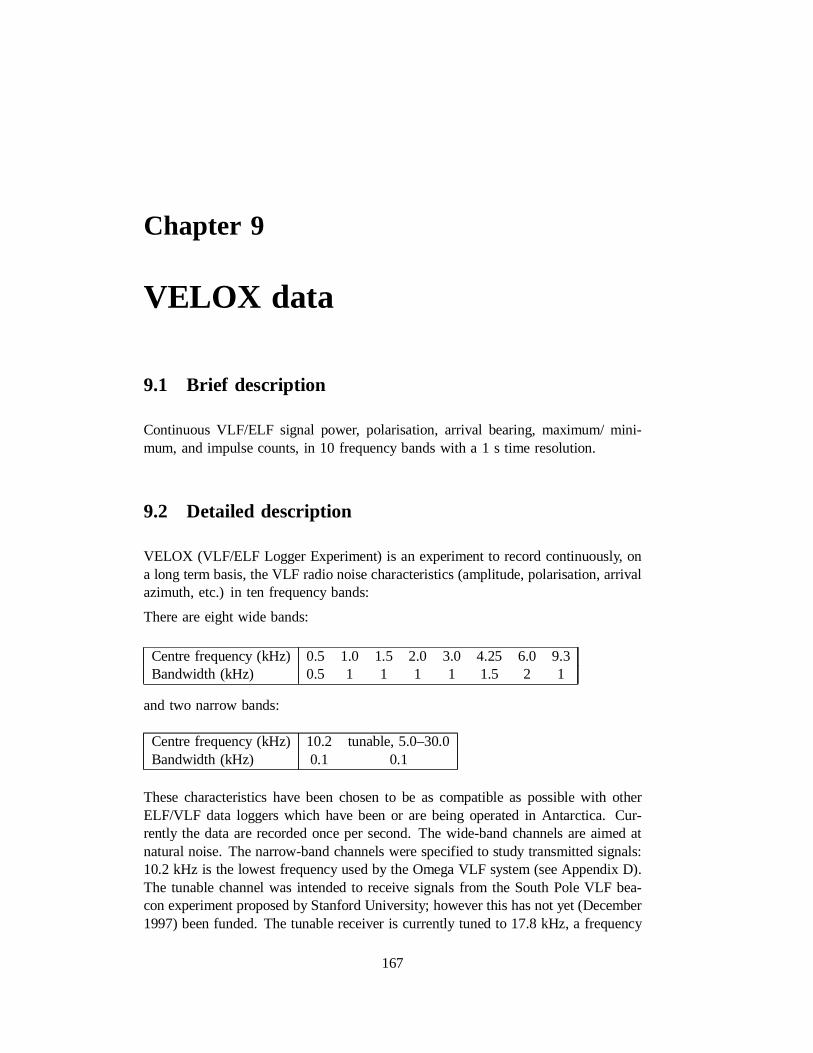
Chapter 9
VELOX data
9.1 Brief description
Continuous VLF/ELF signal power, polarisation, arrival bearing, maximum/ mini-mum, and impulse counts, in 10 frequency bands with a 1 s time resolution.
9.2 Detailed description
VELOX (VLF/ELF Logger Experiment) is an experiment to record continuously, ona long term basis, the VLF radio noise characteristics (amplitude, polarisation, arrivalazimuth, etc.) in ten frequency bands:
There are eight wide bands:
Centre frequency (kHz) 0.5 1.0 1.5 2.0 3.0 4.25 6.0 9.3Bandwidth (kHz) 0.5 1 1 1 1 1.5 2 1
and two narrow bands:
Centre frequency (kHz) 10.2 tunable, 5.0–30.0Bandwidth (kHz) 0.1 0.1
These characteristics have been chosen to be as compatible as possible with otherELF/VLF data loggers which have been or are being operated in Antarctica. Cur-rently the data are recorded once per second. The wide-band channels are aimed atnatural noise. The narrow-band channels were specified to study transmitted signals:10.2 kHz is the lowest frequency used by the Omega VLF system (see Appendix D).The tunable channel was intended to receive signals from the South Pole VLF bea-con experiment proposed by Stanford University; however this has not yet (December1997) been funded. The tunable receiver is currently tuned to 17.8 kHz, a frequency
167
168 CHAPTER 9. VELOX DATA
used by an earlier logger at Halley (see Chapter 3).
The aims of the experiment are:
1. To investigate the occurrence and properties of various kinds of ELF/VLF noiseat Halley, particularly those generated in the magnetosphere (Dudeney et al.,1995, 1997).
2. As part of the GGS (Global Geospace Science) mission (Russell, 1995), forwhich BAS has Principal Investigator status, to investigate various kinds ofinteractions in the magnetosphere by comparing the VELOX output for certainevents, with data from other sensors at Halley, from other ground stations, andon the GGS satellites.
3. As part of BAS’s commitment to the GGS mission, to provide key parameters(1 kHz and 3 kHz power, at 1 minute averages) for insertion into the GGSdatabase.
4. To provide long-term quantitative monitoring of ELF/VLF noise levels andcharacteristics, for global change studies. The data are compatible with thosefrom earlier loggers at Halley, such as the ‘AVDAS-I logger’ (Jenkins, 1988;Smith and Jenkins 1997) (see Chapter 3).
The data parameters are divided into two sets:
Phase 1All the wide-band channels except the impulse counter data. Available inall VELOX data files.
Phase 2The impulse counter data (which are available only for the 3 kHz and9.3 kHz channels) and the narrow-band channels. Available only in data takenwith the new VELOX Phase 2 system, installed at Halley in January 1997.
The measured parameters for each channel are as follows (for exact definitions, seeSmith (1995)):
Scalar describing the mean log amplitude of the waves observed in each frequencyband.
Azimuth describing the mean arrival bearing of the waves.
Ellipticity describing the polarisation.
Peak describing the maximum intensity observed in a specified interval.
Min describing the minimum intensity observed.
Impulse (3 kHz and 9.3 kHz only) describing the number of times per second thatthe intensity increases above three specified thresholds.
9.3. INSTRUMENT/SENSOR 169
9.3 Instrument/sensor
The VELOX system was engineered and manufactured by High Greave Associates(HGA), Sheffield, and is fully described in their manual. The system consists of thefollowing components:
1. The HGA DSP-II Digital Processing System hardware (essentially the same asthe AVDAS hardware). Inputs to the DSP-II are the two broadband analoguesignals from the north-south and east-west VLF loop aerials.
2. Firmware for the DSP-II which contains quite different DSP code from AVDAS.
3. A PC host. Software resides on the host to control the operation of the DSP-II,and the saving of data files.
9.4 Recording method
The two complex auto-spectra and the cross-spectrum of the two broadband VLF inputsignals are calculated by the DSP-II. They are combined to give a scalar power and avector power (see Smith, 1995). The former is used to derive the mean log amplitudeand does not make any allowance for spherics; the latter yields the polarisation andarrival bearing (azimuth), and spectra affected by spherics are excluded. The peakand minimum power, and the impulse count rates above three different thresholds(3 kHz and 9.3 kHz channels only), are also recorded. Details are given in theHGAVELOX Manual.
The VELOX VLXLOGlogger programme runs on the VELOX host PC with appro-priate settings. The computer controls the DSP-II, receives the data, and writes themto disc. GGS key parameter files are transferred to HQ, via the satellite data link,once per week, and then passed on to the GGS CDHF at NASA.
The times written in the file are taken from the IRIG-B time code input to the DSP-II. Originally this was obtained from a time code generator, driven by a rubidiumstandard, but is now (since early 1997) derived from GPS.
9.5 Recording sites
Halley.
A version of VELOX, but with a lower data rate, has been deployed on the BASAGOs (Automatic Geophysical Observatories) to extend VLF observations polewardsfrom Halley into the auroral zone and polar cap. See Chapter 10.
170 CHAPTER 9. VELOX DATA
9.6 Dates/ times
24 hours a day from 14 January 1992; at first a 1 minute sampling time was used,later changed to 10 s. After the system had been fully checked out, the sampling timewas changed to 1 s, on 23 January 1992. During the first four years of operation,1992–1995, the overall data coverage was more than 97%.
9.7 Physical media
Originally (1992–95) the data files were written to the local hard disc of the VELOXhost PC and later archived to 800 M-byte WORM optical discs. From 1996 onwards,all data have been transferred over the Halley LAN to a temporary filespace on theHalley UASD data server (‘Zeus’) and later moved to DAT tape using ARCSERVEsoftware.
9.8 Format description
VELOX and GGS data are stored in files with the same basic format, in data recordscontaining one minute blocks of data. Pre-1997 data files contain only phase 1 datarecords. The VELOX phase 1 data records have the same structure as the GGS datarecords, the only difference being that certain items in the header records are differentto reflect the different number of channels and sampling rates (GGS files contain only1-minute averaged data for the 1 kHz and 3 kHz channels).
Post-1997 data files contain two types of record interleaved in the file, one containingthe phase 2 data and the other the original phase 1 data. The phase 2 data are locatedbefore the corresponding phase 1 data, so that an analysis programme, having readsome phase 2 data, can assume that phase 1 data will follow immediately. If phase1 data are found first, it can assume that it is processing an old file without phase 2data.
The type of a data record is indicated by the first byte of the record. The followingrecord types are defined within the VELOX and AGO-VELOX systems.
A Uncompressed filtered channel (phase 1) data
B Uncompressed spectrogram data (proto-AGO)
C Filtered channel data with abbreviated header (AGO-VELOX)
D Compressed spectrogram data (AGO-VELOX)
E End of logical file marker
F Uncompressed filtered channel (phase 2) data
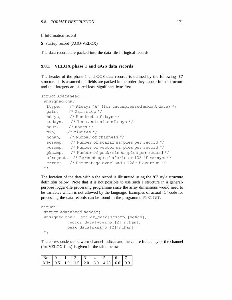
9.8. FORMAT DESCRIPTION 171
I Information record
S Startup record (AGO-VELOX)
The data records are packed into the data file in logical records.
9.8.1 VELOX phase 1 and GGS data records
The header of the phase 1 and GGS data records is defined by the following ‘C’structure. It is assumed the fields are packed in the order they appear in the structureand that integers are stored least significant byte first.
struct Adatahead –unsigned char
ftype, /* Always ’A’ (for uncompressed mode A data) */gain, /* Gain step */hdays, /* Hundreds of days */tudays, /* Tens and units of days */hour, /* Hours */min, /* Minutes */nchan, /* Number of channels */scsamp, /* Number of scalar samples per record */vcsamp, /* Number of vector samples per record */pksamp, /* Number of peak/min samples per record */sfreject, /* Percentage of sferics + 128 if re-sync*/error; /* Percentage overload + 128 if overrun */
";
The location of the data within the record is illustrated using the ‘C’ style structuredefinition below. Note that it is not possible to use such a structure in a general-purpose logger-file processing programme since the array dimensions would need tobe variables which is not allowed by the language. Examples of actual ‘C’ code forprocessing the data records can be found in the programmeVLXLIST .
struct –struct Adatahead header;unsigned char scalar_data[scsamp][nchan],
vector_data[vcsamp][2][nchan],peak_data[pksamp][2][nchan];
";
The correspondence between channel indices and the centre frequency of the channel(for VELOX files) is given in the table below.
No. 0 1 2 3 4 5 6 7kHz 0.5 1.0 1.5 2.0 3.0 4.25 6.0 9.3
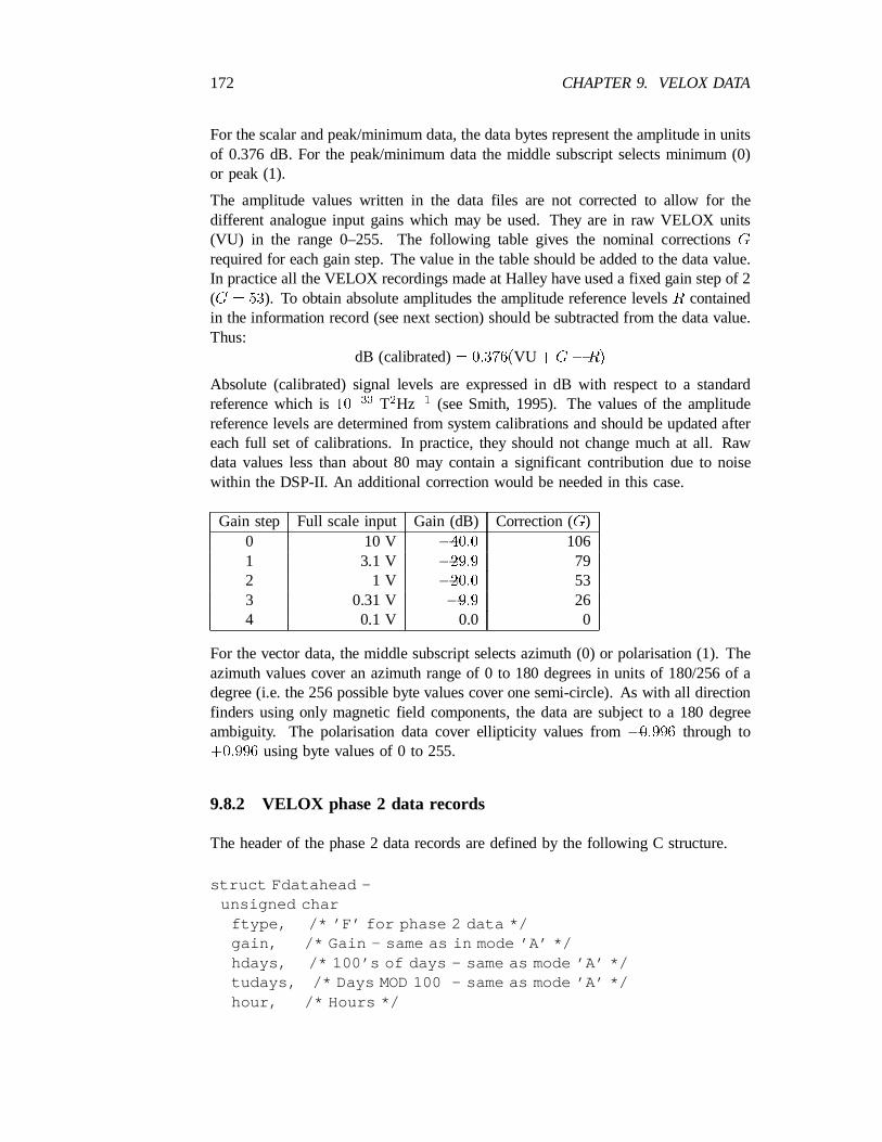
172 CHAPTER 9. VELOX DATA
For the scalar and peak/minimum data, the data bytes represent the amplitude in unitsof 0.376 dB. For the peak/minimum data the middle subscript selects minimum (0)or peak (1).
The amplitude values written in the data files are not corrected to allow for thedifferent analogue input gains which may be used. They are in raw VELOX units(VU) in the range 0–255. The following table gives the nominal correctionsG
required for each gain step. The value in the table should be added to the data value.In practice all the VELOX recordings made at Halley have used a fixed gain step of 2(G = 53). To obtain absolute amplitudes the amplitude reference levelsR containedin the information record (see next section) should be subtracted from the data value.Thus:
dB (calibrated)= 0:376(VU +G¡R)
Absolute (calibrated) signal levels are expressed in dB with respect to a standard¡33 2 ¡1reference which is10 T Hz (see Smith, 1995). The values of the amplitude
reference levels are determined from system calibrations and should be updated aftereach full set of calibrations. In practice, they should not change much at all. Rawdata values less than about 80 may contain a significant contribution due to noisewithin the DSP-II. An additional correction would be needed in this case.
Gain step Full scale input Gain (dB) Correction (G)0 10 V ¡40:0 1061 3.1 V ¡29:9 792 1 V ¡20:0 533 0.31 V ¡9:9 264 0.1 V 0.0 0
For the vector data, the middle subscript selects azimuth (0) or polarisation (1). Theazimuth values cover an azimuth range of 0 to 180 degrees in units of 180/256 of adegree (i.e. the 256 possible byte values cover one semi-circle). As with all directionfinders using only magnetic field components, the data are subject to a 180 degreeambiguity. The polarisation data cover ellipticity values from¡0:996 through to+0:996 using byte values of 0 to 255.
9.8.2 VELOX phase 2 data records
The header of the phase 2 data records are defined by the following C structure.
struct Fdatahead –unsigned char
ftype, /* ’F’ for phase 2 data */gain, /* Gain - same as in mode ’A’ */hdays, /* 100’s of days - same as mode ’A’ */tudays, /* Days MOD 100 - same as mode ’A’ */hour, /* Hours */
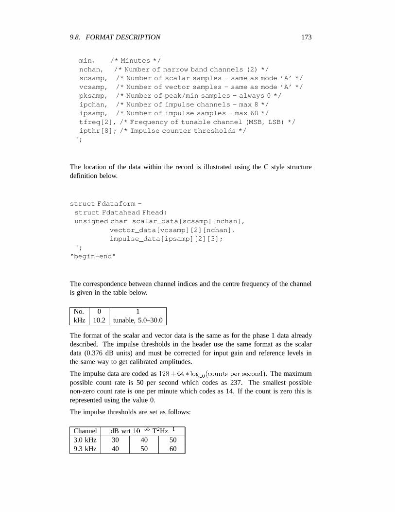
9.8. FORMAT DESCRIPTION 173
min, /* Minutes */nchan, /* Number of narrow band channels (2) */scsamp, /* Number of scalar samples - same as mode ’A’ */vcsamp, /* Number of vector samples - same as mode ’A’ */pksamp, /* Number of peak/min samples - always 0 */ipchan, /* Number of impulse channels - max 8 */ipsamp, /* Number of impulse samples - max 60 */tfreq[2], /* Frequency of tunable channel (MSB, LSB) */ipthr[8]; /* Impulse counter thresholds */
";
The location of the data within the record is illustrated using the C style structuredefinition below.
struct Fdataform –struct Fdatahead Fhead;unsigned char scalar_data[scsamp][nchan],
vector_data[vcsamp][2][nchan],impulse_data[ipsamp][2][3];
";“begin–end"
The correspondence between channel indices and the centre frequency of the channelis given in the table below.
No. 0 1kHz 10.2 tunable, 5.0–30.0
The format of the scalar and vector data is the same as for the phase 1 data alreadydescribed. The impulse thresholds in the header use the same format as the scalardata (0.376 dB units) and must be corrected for input gain and reference levels inthe same way to get calibrated amplitudes.
The impulse data are coded as128+64 ¤ log (counts per second). The maximum10
possible count rate is 50 per second which codes as 237. The smallest possiblenon-zero count rate is one per minute which codes as 14. If the count is zero this isrepresented using the value 0.
The impulse thresholds are set as follows:
¡33 2 ¡1Channel dB wrt10 T Hz3.0 kHz 30 40 509.3 kHz 40 50 60
174 CHAPTER 9. VELOX DATA
9.8.3 Information record
The format of the information record is described by the ‘C’ structure below. A singleinformation record is written at the start of each file. The information contained iscurrently the year in which the data were recorded, the site at which they wererecorded and integers giving the amplitude reference levels. The information in therecord may be displayed using theVLXLIST programme (see below). The recordis padded with zeros to a size of 512 bytes. This is to ensure that there are nocarriage-return line-feed sequences within the first 512 bytes of the data files; this isrequired for network file transfer (TFA) software to identify the file as binary.
struct infoform –unsigned char ftype, /* ’I’ for information record */
iyear, /* year - 1900 */site[8], /* 8 char site name */
int reflevs[3][8]; /* Amplitude ref levelsfor phase 1, narrow band,and impulse. */
unsigned char padding[444]; /* Make up total size to510 */
int reserved[4];";
9.8.4 Data file logical record structure
The data (and information) records are placed in binary data files in logical recordswhich consist of the structures specified in the foregoing sections, preceded by a 16-bit integer specifying the length of the record (not including the length field itself).
The end of the valid data in the file is marked by a record with the character ‘E’ inthe ‘ftype’ field.
9.9 Size of data structures
One VELOX file and one GGS (key parameter) file are recorded each 24 hoursbeginning at 00 UT.
For VELOX files the sampling interval is 1 s for all parameters (Scalar, Vector,Peak/Min, and Impulse counts), but see above for the start of operations in 1992.For the GGS file, only one minute scalar data for two channels (1.0 and 3.0 kHz)out of the eight VELOX channels are recorded. Complete 24-hour phase 1 VELOXfiles should be 3477504 bytes (3396 k-bytes) long and GGS files 24576 bytes (24 k-bytes) long. Phase 2 VELOX files should be 4548038 bytes (4441 k-bytes) long.One record corresponds to a minute. There should therefore be 1440 records in a
9.10. VALIDATION 175
24-hr file VELOX phase 1 or GGS file, and 2880 in a VELOX phase 2 file (1440phase 1 data records and 1440 phase 2 data records).
9.10 Validation
For the purpose of verifying data files to ensure they can be read, theVLXLISTprogramme may be used. If this is run with no command line options it will simplyread through the file until an ‘end of logical file’ record is found, and report thenumber of records processed; this should be 1440 for a complete day’s data (2880for phase 2 files).
9.11 Anomalous or suspect data
For a few files, recorded in the first part of 1993, data bits have been “dropped”,resulting in a file becoming corrupt part-way through. These files have all beenrepaired before being archived to CD-ROM.
From probably 26 December 1993 until 24 December 1994 the Halley loop aerials±were incorrectly rigged. The apex angle was 112 instead of a right angle, and the
lower sides were slack and 10.1 m long instead of 7.6 m; the bottom vertex was211.1 m below the top instead of 10.7 m. This gave an estimated area of 90 m per
2loop instead of 58 m , leading to an increase in sensitivity of»3.8 dB. However,the change in size and area of the loops, together with the incorrect positioning ofthe calibration coil (6.7 m below the apex instead of 5.4 m), meant that the mutualimpedance between the calibration coils was incorrect (estimated from calibrationsdone before and after the configuration was corrected in December 1994 to be 20%too low, corresponding to»2 dB) so that the normal calibrations for the VELOXdata during this period should not be trusted. Furthermore, the movement of the slacklower sections in the wind undoubtedly caused increased spurious signal variability.More information can be found in Appendix 1 of theHalley Trip Report 1994–95byA.J. Smith, and in the1994 Halley VLF report(AD6/2Z/1994/I3).
During 1996 there was an apparent increase in background noise which switched onand off intermittently, particularly during the latter part of the year. It was thoughtthat this could be due to a fault in the loop aerial system, possibly poor connectors. Anew system, with different connectors, is being installed during the 1997–98 season.
Some 1996 files, although correctly collected at Halley, had 16 pre-pended extraneousbytes when de-archived from DAT tapes at Cambridge. This is believed to be a bugin the archiving system. Such files are not recognised as valid VELOX files by anyof the VELOX software. The unwanted bytes can be removed using theVELOXFIXprogramme (written by Jon Oldfield):
VELOXFIX ¡input file¿ ¡output file¿ ¡n¿
176 CHAPTER 9. VELOX DATA
where ¡input file¿ and ¡output file¿ are the source and destination datafiles and¡n¿ is the number of bytes of data to be removed. For example,
VELOXFIX vlx97164.dat vlx97164.new 16
In 1997, incorrect impulse thresholds (20, 40, 60, 20, 40, 60) were used until 9 April(day 99).
In 1997, incorrect reference values were used until 13 June (day 164).
In 1997, the tunable receiver was changed from 10.2 kHz to 17.8 kHz on 13 June(day 164).
9.12 Calibration
9.12.1 Full calibrations
The twice yearly main calibration procedure for the VLF system as a whole at Halley,described in theHalley VLF Manualand documented by calibration forms, servesalso to calibrate VELOX which is kept running throughout. The calibrations can beanalysed usingVLXLIST . Full calibrations were done at the time of installation inJanuary 1992; seeHalley VLF Installation Report, 1991–92, and subsequent annualreports. A special procedure using simulated impulses is needed to calibrate theimpulse channels; this is being developed during 1997.
9.12.2 VELOX calibration checks
The regular automatic digital calibration tones provide a useful way of checking thecalibration of VELOX throughout the year. The 10 s long tones that occur everyhour are most suitable. All calibration tones are blanked out from the normal plotsproduced byVLXPLOT. The data can most easily be examined usingVLXLIST ; theHalley VLF Manual(1995) suggests how this can be done. As part of the verificationof VELOX files, the data values during the 0000 UT calibration tone should be listedand recorded in the log book once or twice per week. The nominal data valuesduring the calibration tones and those typically observed (values from 1992, day 27,0000 UT) are listed below.
Channel 1 kHz 1.5 kHz 2 kHz 4.25 kHzNominal amplitude 53.6 dB 54.8 dB 53.0 dB 51.2 dBTypical amplitude 54.1 dB 56.4 dB 53.4 dB 51.5 dB
± ± ± ±Nominal azimuth 45.0 45.0 45.0 45.0± ± ± ±Typical azimuth 41.5 40.8 40.1 40.1
9.13. NAMING/NUMBERING CONVENTIONS 177
9.13 Naming/numbering conventions
Normally files will have the namesVLXyyddd.DAT and GGSyyddd.DAT whereyy stands for the last two digits of the year andddd for the day of year number.
9.14 Catalogues
Catalogues are produced usingVLXLIST . Catalogue files are returned monthly fromHalley, and stored on the UASD network file server in directories of the formo:“uasd“wave“data“catlogs“veloxcat“halley“1997 . A fragment ofone such file,vlxmay97.cat , is given below:
’VLX97121.DAT’, Halley, 1997 121 0000.Narrowband channels: 2, reference levels: 73 73Impulse channels: 6, reference levels: 80 80 80 73 73 73Wideband channels: 8, reference levels: 57 75 77 81 80 82 84 732880 records processed.
’GGS97121.DAT’, Halley, 1997 121 0000.Wideband channels: 2, reference levels: 75 801440 records processed.
Consolidated annual catalogues, e.g.vlx93.cat have been produced, as well as Lo-tus 1-2-3 spreadsheet files of the typevlx93.wk1 which provide coverage statisticsfor the year.
9.15 Analysis methods
Analysis is done on a PC using the MS-DOS software described below. At presentthe data are accessed from a local CD-ROM drive, but future developments maymake it possible to have the data stored on a central on-line server, and available ondemand.
9.16 Analysis software
9.16.1 Overview
The following are available:
VLXLIST Lists data files in numerical form to the screen, a printer, or a disc file.
VLXPLOT Produces a graphical representation of the data on the screen or a graphicsfile (which may then be imported into WordPerfect, for example).
178 CHAPTER 9. VELOX DATA
VLXCOPYFor manipulating data files.
VLXSPECProduces a pseudo-spectrogram representation, in colour, on the screen,or on paper (using a HP Paintjet colour ink-jet printer or any colour PostScriptprinter).
9.16.2 VLXLIST
TheVLXLIST programme is for listing in text format the data in VELOX files. Theoutput from the programme is normally displayed on the screen but may be redirectedto a file or printer using the standard DOS redirection facility (¿ or ¿¿). For eachfile the output contains a header giving the recording site, date and time of the firstdata record followed by a listing of the data requested. The data are listed in separateblocks for each record in the file and each parameter.
The command syntax is as follows:
VLXLIST file-name [options]
wherefile-name is the name of the VELOX data file (which may include wild-cards). If no options are specified, the information in the information record at thebeginning of the file, and the number of records in the file, are listed, e.g.
’VLX97119.DAT’, Halley, 1997 119 0000.Narrowband channels: 2, reference levels: 73 73Impulse channels: 6, reference levels: 80 80 80 73 73 73Wideband channels: 8, reference levels: 57 75 77 81 80 82 84 732880 records processed.
If options are specified, they may be any combination of the following.
/D=ddd whereddd is the day number at which to start the listing, and defaults tozero.
/T=hhmm wherehhmmis the time (hours and minutes as a single number) at whichto start the listing, and defaults to zero. Note that for this option to work/Dmust be specified as well.
/N=n wheren is the number of records to be listed and defaults to the whole file.
/F to list the status indicators for each record. These aresf and ov . For thephase 1 records the values represent the gain step and the percentage of spectracontaining spherics and overloads respectively. For the phase 2 records, thegain step and the frequency of the tunable narrow-band channel are listed.
/S to list scalar amplitude (averaged log power) data.
/A to list azimuth data.
9.16. ANALYSIS SOFTWARE 179
/E to list ellipticity data.
/M to list minimum amplitude data.
/P to list peak amplitude data.
/I to list impulse data.
/T to list impulse data threshold values.
/R to list data in raw mode (i.e. no gain correction and no conversion to real units).
/1 to list only phase 1 data (i.e. 0.5 to 9.3 kHz channels).
/2 to list only phase 2 data (i.e. 10.2 kHz and tunable channels, plus impulse data).
The following is an example of the output produced byVLXLIST operating on aphase 1 file, in this case by the command:
VLXLIST VLX92315.DAT /D=315 /T=0317 /F /S /N=1 ¿ VLX92315.OUT
in which the output has been redirected to a file. The header of this example givesthe filename, station (Halley) and year, day, time of the start of the file. In the datathe first three columns are the day number, the hours and minutes as a single number,and the seconds. Next comes an indicator showing what the rest of the columnscontain. This is the same as the command line option letters described above. Thestatus line, markedF, is followed by one minute of scalarS data.
’VLX92315.DAT’, Halley, 1992 315 0000.Wideband channels: 8, reference levels: 57 75 75 83 81 84 85 73315 0317 00 F gain = 2, sc = 4%, ov = 7%, re-sync = 0, overrun = 0
315 0317 00 S 58.66 54.90 57.53 54.52 21.81 52.26 45.50 52.26315 0317 01 S 50.01 39.10 28.95 21.43 20.68 29.70 44.37 51.89315 0317 02 S 53.02 40.98 30.08 22.56 23.69 31.58 46.25 54.52
..... etc. .....315 0317 59 S 51.51 39.86 29.70 22.18 22.56 30.83 47.00 53.77
1 records processed.
The following is an example of output produced byVLXLIST operating on a phase 2file, in this case by the command:
VLXLIST VLX97119.DAT /D=119 /T=0543 /2 /F /T /I /S /N=1 ¿ VLX97119.OUT
As the options/S and /2 are present, the scalar data from the phase 2 records areoutput, i.e. for the fixed and variable narrowband channels. This is followed bythe impulse data, the first three columns corresponding to the three thresholds (inincreasing order) for the 3 kHz channel and the second three columns correspondingto the 9.3 kHz channel. Finally, since/T was specified, the impulse thresholdsthemselves are listed.
180 CHAPTER 9. VELOX DATA
’VLX97119.DAT’, Halley, 1997 119 0000.Narrowband channels: 2, reference levels: 73 73Impulse channels: 6, reference levels: 80 80 80 73 73 73Wideband channels: 8, reference levels: 57 75 77 81 80 82 84 73
119 0543 00 F gain step = 2, tunable channel = 10200 Hz
119 0543 00 S 29.33 32.34119 0543 01 S 36.47 38.35119 0543 02 S 29.33 31.96
..... etc. .....119 0543 59 S 32.71 34.59
119 0543 00 I 0.95 0.59 0.00 0.95 1.00 0.00119 0543 01 I 0.59 0.00 -2.00 0.77 0.77 -2.00119 0543 02 I 0.69 0.00 0.00 1.22 0.95 0.00
..... etc. .....119 0543 59 I 0.47 0.84 -2.00 0.59 0.89 0.47
119 0543 00 T 29.70 39.86 49.63 39.86 49.63 59.78
1 records processed.
Unless the/R option is used, the amplitude data are corrected to allow for the¡33 2 ¡1analogue input gain. Amplitudes are presented in dB relative to10 T Hz
(assuming the correct reference file was loaded into the logger programme), azimuthsin degrees, ellipticity as a number between¡0:99 and+0:99, and impulse data aslog of the counts per second. A value of¡9999 for any parameter indicates that
10
the signal amplitude was too near the system noise level for reliable measurement.
When /R is used, the raw data file values are presented for all parameters.
9.16.3 VLXPLOT
VLXPLOTis a programme to plot VELOX (or GGS) data on the PC screen. Option-ally the output may be written to a file (or series of files) in HPGL format, whichmay be processed and printed. See examples Figs. 9.1–9.3 and Fig. 9.5. The formatof the plot may be varied using command line options which are listed below; as aminimum at least one of/S , /M, /P , /A , /E (or /I if accompanied by/2 ) mustbe specified, otherwise an empty frame with no data (other than status informationin the top panel) will result. The command line syntax is as follows.
VLXPLOT file-name [options]
wherefile-name is the name of the VELOX data file (which may include wild-cards) andoptions may be any combination of the following. These are mostlythe same as theVLXLIST options.
9.16. ANALYSIS SOFTWARE 181
/D=ddd whereddd is the day number at which to start the plot, and defaults tozero.
/T=hhmm wherehhmmis the time (hours and minutes as a single number) at whichto start the plot, and defaults to zero. Note that for this option to work/Dmust be specified as well.
/N=n wheren is the number of frames to be plotted, and defaults to the maximumvalue, 32767 (i.e. in practice the whole file).
/S to plot scalar amplitude (averaged log power) data.
/A to plot azimuth data.
/E to plot ellipticity data.
/M to plot minimum amplitude data.
/P to plot peak amplitude data. It is recommended that the options/S , /M and /Pare not mixed with/A , or /E as this causes some labelling conflicts.
/MINAMP=min and /MAXAMP=maxto specify the range of the amplitude plots(/S /M /P ) in dB. The default is 10 to 70 dB.
/MINAZ=min and /MAXAZ=max to specify the range of the azimuth plot (/A ) indegrees. The default is 0 to 180 degrees.
/MINEL=min and /MAXEL=max to specify the range of the ellipticity plot (/E ).The default is¡1:0 to +1:0.
/NSC (no suppress cal) to plot data without suppressing calibration tones.
/R to plot data in raw mode (i.e. no gain correction applied).
/X=n to set theX-axis (time) scale factor.n is the number of plotter units perminute and may take values between 6 (24 hours of data on one frame) and4800 (two minutes of data on one frame). The default is 16.
/O=fffff to plot to a series of files in HPGL format. The files are namedfffff000.GRF , fffff001.GRF and so on. If/O is not specified, theplot is produced on the PC screen.
/I=n to number the files produced by/O starting fromn rather than 0.
/1 or /2 to plot VELOX phase 1 (default) or phase 2 data. Phase 1 data compriseeight wideband channels (except the impulse parameter), whilst phase 2 datacomprise the two narrow band channels (i.e. 10.2 kHz and tunable channels)plus the impulse parameters for 3.0 and 9.3 kHz.
/V To plot 10 second averages. This runs faster and produces a smoother plot.
182 CHAPTER 9. VELOX DATA
A narrow box at the top of the plot shows thesf (sferics) andov (overloads) statusindicators. The height of the box corresponds to a range of 0 to 10%. A colourmonitor (or plotter) is necessary in order to be able to distinguish unequivocallybetween the two indicators, although in normal operationsf should always be higherthanov .
The other eight boxes each correspond to one frequency band. If the data file containseight bands, then the boxes are labelled with the standard VELOX frequencies. Sim-ilarly if the data file contains two bands, the boxes will be labelled with the standardGGS frequencies. If/2 is selected and the data file contains two narrowband plussix impulse channels, the boxes will again be labelled appropriately. The labels willinclude impulse threshold levels taken from the first data record of the frame.
The selected parameters are plotted within each box with the height of the box±corresponding to default ranges of 10 dB to 70 dB for amplitude, 0 to 180 for
azimuth,¡1 to +1 for ellipticity, and¡2:0 to +2:0 [log(counts=second)] for theimpulse channels, unless set otherwise usingMAXAMP, MINAMP, etc. Each parameteris plotted in a different colour, with an indicator at the top of the frame to show whichcolour represents which parameter.
9.16.4 VLXCOPY
VLXCOPYis a programme to copy parts of one or more VELOX or GGS logger filesto a new file. It can optionally perform format conversion on VELOX files. Thecommand syntax is:
VLXCOPY input-file1 [input-file2] .... output-file
The output file is always the last parameter on the line; the programme opens thisfirst so that it has somewhere to write the data from the input files. The output filemust not already exist.
In addition to the files names, option strings may appear at various positions on thecommand line. Both the position and case of option strings is important.
Format conversion options should be first on the command line before any file namesor other options. These may be:
/WC=wideband-channel-list default is no wideband data/NC=narrowband-channel-list default is no narrowband data/IC=impulse-channel-list default is no impulse data/S=scalar-interval default is 60 seconds/V=vector-interval default is 60 seconds/P=peak/minimum-interval default is 60 seconds/I=impulse-interval default is 60 seconds

9.16. ANALYSIS SOFTWARE 183
At least one of the/WC, /NC or /IC options must be specified if format conversion isrequired (if not, all data are copied verbatim). Thechannel-listis a string of channelnumbers with no spaces such as01234567 . The only allowable values for/S , /V ,/P and /I are 60 for one sample per minute, or any number greater than 60 for nodata. The same format conversion is applied to all input files.
After the format conversion options, but before any file names, a file list option mayappear to specify the name of a file containing a list of input files (one per line).This is useful if the number of input files required is too large to fit on the commandline. The syntax is:
/f=filename
Data selection options may be placed after each input file name and apply only tothat particular file. They may appear either on the command line or after the inputfile names in a file list file. The syntax is:
/s=skip/n=count
The skip parameter is the number of data records (one per minute for phase 1 only,two per minute for files containing phase 1 and phase 2 data) that will be skippedbefore starting to copy data to the output file. It defaults to zero. Thecountparameterspecifies the maximum number of data records that will be copied to the output file.It defaults to the whole file (actually 32767). The skip and number parameters referto the file immediately on their left. These parameters must be specified separatelyfor each input file if required.
The information record from the first input file only is copied to the output file.Information records from other files are checked and a warning message issued ifthey are different. If the information record from a different file is required then thisfile should be specified first with/n=0 .
The data from each file are copied until the specified number of records have beencopied, an ‘end of logical file’ record is found, the DOS reports end of file, or anerror occurs. In the event of a DOS end of file (which should not happen) or anerror, a warning message will be issued. The programme will then move on to thenext input file if there is one.
Note thatVLXCOPYdoes not attempt to update the reserved section of the data fileinformation record used internally byVLXLOG. This means thatVLXLOGwould notbe able to re-open an output file fromVLXCOPYand append more data to it.
The skip and count options ofVLXCOPYmay be used to repair corrupt files, as inthe batch fileRPR95068.BAT shown below.
@ECHO OFFREM To repair VELOX file VLX95068.dat AJS 6 Nov 96REM Minute 0928 corrupt
184 CHAPTER 9. VELOX DATA
VLXCOPY VLX95068.DAT /n=567 VTEMP1.DATVLXCOPY VLX95068.DAT /s=568 VTEMP2.DATVLXCOPY VTEMP1.DAT VTEMP2.DAT VTEMP.DATDEL VLX95068.DATREN VTEMP.DAT VLX95068.DATDEL VTEMP1.DATDEL VTEMP2.DAT
9.16.5 VLXSPEC
VLXSPECis a programme to plot the wideband channels of the VELOX data in spec-trogram form. It is not applicable to narrowband or impulse data. The result maybe displayed on the PC screen or written to a file (or series of files) in ‘AV-GRAF’format. The resulting files may then be plotted on a suitable hard-copy device (e.g.the HP PaintJet usingPLOTHPPor any PostScript printer usingPLOTPS, see Ap-pendix E). An example is shown in Fig. 9.4. The format of the plot may be variedusing command line options which are listed below. The command line syntax is asfollows.
VLXSPEC file-name [options]
wherefile-nameis the name of the VELOX data file (which may include wild cards)andoptionsmay be any combination of the following. These are mostly the same astheVLXPLOToptions.
/D=ddd whereddd is the day number at which to start the plot, and defaults tozero.
/T=hhmm wherehhmmis the time (hours and minutes as a single number) at whichto start the plot, and defaults to zero. Note that for this option to work/Dmust be specified as well.
/N=n wheren is the number of frames to be plotted, and defaults to 32767 (i.e. inpractice the whole file).
/S (default) to plot scalar amplitude (averaged log power) data.
/A to plot azimuth data.
/E to plot ellipticity data.
/M to plot minimum amplitude data.
/P to plot peak amplitude data.
/NSC (no suppress cal) to plot data without suppressing calibration tones.
/R to plot data in raw mode (ie. no gain correction applied).
9.17. DERIVED DATA SETS 185
/X=n to set theX axis (time) scale factor.n is the number of plotter units perminute and may take values between 12 (24 hours data on one frame) and 960(18 minutes data on one frame). The default is 16 (18 hours per frame). Forbest resultsn should be a multiple of 16 and a factor of 960.
/O=fffff to plot to a series of files in ‘AV-GRAF’ format. The files are namedfffff000.GRF , fffff001.GRF and so on. If/O is not specified, the plotis produced on the PC screen.
/I=n to number the files produced by/O starting fromn rather than 0.
/MINAMP=min, /MAXAMP=max to specify the range of data values displayed (indB) when amplitude data are selected (/S /M /P ). When azimuth or ellipticitydata are plotted, themin parameter specifies an amplitude threshold. If themean amplitude is below this level, the azimuth or ellipticity will not be plotted.The defaults aremin=10;max=70.
/Q This causes azimuth data to be plotted in high quality mode, where smoothingbetween the frequency bands is used as it is for amplitude and ellipticity. Thedisadvantage is that it runs somewhat slower.
9.17 Derived data sets
Routine plots of the scalar data, at a compressed scale (one or two pages per day)have been done using eitherVLXPLOT, or VLXSPEC, partly as a check on systemperformance and partly to scan for interesting events.
Format-converted files may be created usingVLXCOPY. For example several day-longfiles may be averaged to a lower resolution and concatenated to a multi-day file. SeeSmith (1995) for examples.
GGS key parameter files are converted to a different format (CDF) for transmis-sion to the GGS CDHF, and are also available on the BAS World Wide Web site, athttp://www.nerc-bas.ac.uk/public/uasd/instrums/grasp/intro.html .
9.18 Archiving
Archived data are shipped back from Antarctica in MS-DOS form on DAT tapes(with a back-up). At HQ these are copied to CD-ROM for permanent archiving andscientific use. See Appendix A for further information. A CD-ROM catalogue can befound in the WAVE area of the UASD server. This catalogue, for years 1992–1996,which can be found as fileVLXCDROM.TXT, is reproduced below.
VELOX CD-ROM Catalogue:————————————————CD-ROM Files
186 CHAPTER 9. VELOX DATA
————————————————VLX_VELOX_2000_A VLX92014.DAT to VLX92120.DATVLX_VELOX_2001_B VLX92121.DAT to VLX92225.DATVLX_VELOX_2002_A VLX92226.DAT to VLX92334.DATVLX_VELOX_2003_B VLX92335.DAT to VLX92366.DATVLX_VELOX_2004_A VLX93001.DAT to VLX93110.DATVLX_VELOX_2005_B VLX93111.DAT to VLX93214.DATVLX_VELOX_2006_A VLX93215.DAT to VLX93326.DATVLX_VELOX_2007_B VLX93327.DAT to VLX93365.DATVLX_VELOX_2008_A VLX94001.DAT to VLX94110.DATVLX_VELOX_2010_A VLX94110.DAT to VLX94218.DATVLX_VELOX_2011_B VLX94219.DAT to VLX94328.DATVLX_VELOX_2012_A VLX94329.DAT to VLX94365.DATVLX_VELOX_2113_A VLX95001.DAT to VLX95107.DATVLX_VELOX_2114_B VLX95108.DAT to VLX95212.DATVLX_VELOX_2115_A VLX95213.DAT to VLX95313.DATVLX_VELOX_2116_B VLX95314.DAT to VLX95365.DATVLX_VELOX_2117_B VLX96001.DAT to VLX96182.DATVLX_VELOX_2118_A VLX96183.DAT to VLX96366.DAT
9.19 Documentation
² VELOX ManualHigh Greave Associates, Sheffield, January 1996 (RevisedApril 1996)
² Installation of the VLF Experiments at Halley-5, 1991–92A.J. Smith (BASReport ZV/1991/I3).
² Halley VLF ManualA.J. Smith and J. Digby, June 1995.
9.20 References
² Dudeney J.R., Rodger A.S., Smith A.J., Jarvis M.J. and Morrison K. (1995)Satellite Experiments Simultaneous with Antarctic Measurements (SESAME).Space Sci. Rev.71, 705–742.
² Dudeney J.R., Horne R.B., Jarvis M.J., Kressman R.I., Rodger A.S. and SmithA.J. (1997) British Antarctic Survey’s ground-based activities complementaryto satellite missions such as Cluster, In Satellite-ground based coordinationSourcebook, Edited by M. Lockwood, M.N. Wild, and H.J. Opgenoorth, ESASpecial PublicationSP-118, 101–109.
² Jenkins P.J. (1988) A survey of ELF/VLF noise at Halley, Antarctica, andassociated studies. Ph.D. thesis, University of Sheffield.
² Russell .C.T. (Ed.) (1995) The Global Geospace Mission, Kluwer AcademicPublishers, Dordrecht, Netherlands.
9.20. REFERENCES 187
² Smith A.J. (1995) Report on trip to Halley 1994/1995 season. (Internal BASreport)
² Smith A.J. (1995) VELOX: a new VLF/ELF receiver in Antarctica for theGlobal Geospace Science mission. J. Atmos. Terr. Phys.57, 507–524.
² Smith A.J. and Jenkins P.J. (1998) A survey of natural electromagnetic noisein the frequency rangef = 1–10 kHz at Halley station, Antarctica: 1. Radioatmospherics from lightning, J. Atmos. Solar-Terr. Phys.60, 263–277.
Chapter 10
AGO-VELOX data
10.1 Brief description
Continuous VLF/ELF signal power, polarisation, arrival bearing and maximum/ min-imum, in 5 frequency bands with a 1 s time resolution (for power, and 10 s for theother parameters). Sampled broadband data (‘snapshot mode’) every 15 minutes.
10.2 Detailed description
The AGO-VELOX is a version of the full VELOX system which has operated atHalley since January 1992 (see Chapter 9). It has been designed to work on the BASAGO (Automatic Geophysical Observatory) platform (Dudeney et al., 1995; Dudeneyet al., 1998), and has a lower data rate than the Halley system, because of power andon-board data storage limitations.
In conjunction with other instruments on the BAS AGO platform (e.g. riometer,magnetometer, photometer), the scientific aims will be:
1. to provide information about
(a) positions and shapes of magnetospheric boundaries, and
(b) energy deposition into the ionosphere/atmosphere, and the time rate ofchange of these quantities;
2. to be used in studies of magnetosphere-ionosphere coupling, substorms, auroralprocesses, etc.
3. to investigate plasma wave generation, propagation, amplification, damping etc.at high latitudes.
The data are of two types:
188
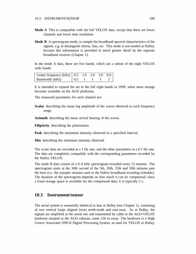
10.3. INSTRUMENT/SENSOR 189
Mode A This is compatible with the full VELOX data, except that there are fewerchannels and lower time resolution
Mode B A spectrogram mode, to sample the broadband spectral characteristics of thesignals, e.g. to distinguish chorus, hiss, etc. This mode is not needed at Halley,because this information is provided in much greater detail by the separatebroadband receiver (Chapter 1).
In the mode A data, there are five bands, which are a subset of the eight VELOXwide bands:
Centre frequency (kHz) 0.5 1.0 2.0 3.0 6.0Bandwidth (kHz) 0.5 1 1 1 2
It is intended to expand the set to the full eight bands in 1999, when more storagebecomes available on the AGO platforms.
The measured parameters for each channel are:
Scalar describing the mean log amplitude of the waves observed in each frequencyrange.
Azimuth describing the mean arrival bearing of the waves.
Ellipticity describing the polarisation.
Peak describing the maximum intensity observed in a specified interval.
Min describing the minimum intensity observed.
The scalar data are recorded at a 1 Hz rate, and the other parameters at a 0.1 Hz rate.The data are completely compatible with the corresponding parameters recorded bythe Halley VELOX.
The mode B data consist of a 0–6 kHz spectrogram recorded every 15 minutes. Thespectrogram starts at the 30th second of the 5th, 20th, 35th and 50th minutes pastthe hour (i.e. the synoptic minutes used in the Halley broadband recording schedule).The duration of the spectrogram depends on how much it can be compressed, sincea fixed storage space is available for the compressed data; it is typically 2 s.
10.3 Instrument/sensor
The aerial system is essentially identical to that at Halley (see Chapter 1), consistingof two vertical loops aligned (true) north-south and east-west. As at Halley, thesignals are amplified at the aerial site and transmitted by cable to the AGO-VELOXhardware situated in the AGO caboose, some 120 m away. The hardware is a HighGreave Associates DSP-II Digital Processing System, as used for VELOX at Halley,
190 CHAPTER 10. AGO-VELOX DATA
but adapted slightly for use on the AGO. The analogue input signals are digitised andthen processed by the DSP chip under the control of the specialised AGO-VELOXfirmware to produce the required data. To guard against the possibility that theAGO-VELOX might become stuck in a corrupted state, from 1997 it automaticallyreboots itself once per day (actually once every 23 hours 55 minutes). This causesthe loss of five minutes mode A (filtered channel) data for each restart. The modeB (spectrogram) data should not be affected. Full details are provided in HGA’sAGO-VELOX Manual, and theBAS AGO-VELOX Manual.
10.4 Recording method
The data are sent from the AGO-VELOX instrument to the main AGO system.Timing information, derived from GPS, is passed in the reverse direction.
10.5 Recording sites
When the BAS AGO network is fully developed, it is planned that there will be anAGO-VELOX at each of the four sites: A80, A81, A84, A77 (see Appendix C forthe coordinates).
10.6 Dates/ times
The A80 AGO-VELOX began operating on 17 January (day 17) 1995 at 2000 UT,and data exist from then until 26 February (day 57) 1995 at 2100 UT, when the AGOpower supply failed. Operation resumed on 21 January (day 21) 1996 at 1730 UT.There are data gaps when there is no power available to run the instrument. Thistypically occurs for short periods in winter, when the batteries have discharged andthere is no wind to turn the wind generator.
The A81 AGO-VELOX began operating on 14 January (day 14) 1996 at 1700 UT
The A84 AGO-VELOX is scheduled for installation during the 1998–99 season.
10.7 Physical media
Data are recorded at the AGO site, and collected each year. Currently optical discs areused as the recording medium. At Cambridge the data are transferred to CD-ROM.
10.8. FORMAT DESCRIPTION 191
10.8 Format description
10.8.1 Logical records
All data are stored in logical records with the following format. There may be otherbytes in the files between logical records.
Field Size ContentsSync pattern 2 0x01, 0x44Length (n) 2 lsb, msb (10246 max)Data nChecksum 1 modulo 256 sum of all bytes
excluding first sync byte
10.8.2 Mode A data format
The AGO-VELOX mode A data has an abbreviated header. Most items with fixedvalues (number of channels, sampling rates, etc.) are omitted and their value impliedby the type field. Format ‘C’ (0x43 ) implies 5 channels, 5 minute records, 1 secondsampling for averaged amplitude (scalar) data, 10 second sampling for peak/minimumand vector data, 32-bit binary time. The following C structure defines the format.
struct Adataform –unsigned char
ftype, /* 0x43 for mode A data */gain, /* Analog gain index */time_bytes[4], /* Time as 32bit seconds */sfreject, /* Sferic reject count */error, /* Error flag */Cdata[(SCNSAMP + PKNSAMP*2 + VCNSAMP*2) * NUMCHAN];
";
10.8.3 Mode B data format
The mode B (spectrogram) data are a variable number of spectra with 50 Hz frequencyresolution and 10 ms time resolution. The spectra are coded with 5 bits per spectrumpoint representing a range of 93 dB in 3 dB steps and 120 points per spectrum. The5 bit data are then compressed using a loss-less compression algorithm (a variant ofLempel-Ziv) and as many spectra as possible written to the data field of the format.The maximum number of spectra is 256 and in the (unlikely) event that these all fitin the format, the remaining space will be padded with zeros.
struct Ddataform –
192 CHAPTER 10. AGO-VELOX DATA
unsigned charftype, /* 0x44 for mode B data */serno, /* Instrument serial number */time_bytes[4], /* Time as 32bit seconds */Ddata[10239], /* Data as a bit stream */numspec; /* Number of spectra / 2 */
";
10.8.4 Start-up record
Whenever the AGO-VELOX is powered up, or a watch-dog or periodic reset occurs,a record with the following structure is sent to the AGO system.
struct Sdataform –unsigned char
ftype, /* ’S’ for startup record */serno, /* Instrument serial number */chk_sum[2], /* EPROM checksum, lsb, msb */start_flag[2], /* Start up reason flag */addr_bytes[2], /* Memory fault addr, lsb first */mem_pattern, /* Memory test pattern */mem_error, /* Memory test bits read back */volt_mon[6]; /* Voltage monitors */
";
The correspondence between site and serial number is:
AGO site A80 A81 A84AGO-VELOX Ser. No. 001 002 003
For data recorded up to and including 1996, thestart flag is always0x0000 . From1997 onwards the flag is undefined (probably zero) if the AGO-VELOX just poweredon, 0x5744 (the ascii codes for “WD”) if the watchdog caused the restart, and0x5052 (“PR”) if a periodic restart occurred.
10.9 Size of data structures
The mode A (filter-bank) data are written in 5-minute records (known as format C)whilst the mode B (spectrogram) records are written every 15 minutes as a format Drecord. [Formats A and B are already used by the VELOX system.] Format C andformat D records have 2108 and 10246 bytes of data, respectively. Each record ispreceded by two synchronisation bytes and two length bytes, and terminated by achecksum byte. Thus the total lengths of the records are2108 + 5 = 2113 and10246 + 5 = 10251 bytes. Start-up records occur whenever the AGO-VELOX is
10.10. VALIDATION 193
powered up or a watchdog reset or periodic restart occurs, but leaving that aside, thelengths of data for various periods of continuous operation are as follows (1 k-byte= 1024 bytes; 1 M-byte = 1024 k-bytes):
Time Length of data bytes k-byte M-byte1 hour (12£ 2113) + (4£ 10251) 66360 64.8 0.11 day 24£ 66360 1592640 1555.3 1.51 week 7£ 1592640 11148480 10887.2 10.61 month 30£ 1592640 47779200 46659.4 45.61 year 365£ 1592640 581313600 567689.1 554.4
N.B. The AGO system for some reason likes data records with an even number ofbytes, and thus adds an extra byte of padding to the end of each of the records beforerecording it.
10.10 Validation
VLFCHECKis a basic data format checking programme written by Dick Kressmann.It is run by inputting an AGO-VELOX file. From the DOS prompt:
VLFCHECK ¡ ago_file
By default the output is shown on the screen and may look something like:
317 bytes skipped searching for record markerRecord type C length 2108 bytesRecord type C length 2108 bytesRecord type C length 2108 bytesRecord type D length 10246 bytesRecord type D length 10246 bytesRecord type C length 2108 bytesChecksum errorRecord type C length 2108 bytesRecord type D length 10246 bytesRecord type C length 2108 bytesRecord type C length 2108 bytes
There should not normally be errors, but the above shows an example of an occasionalone that did occur. For long files it will be more convenient to direct the output ofthe programme to a file
VLFCHECK ¡ ago_file ¿ check_file
and then examine this with an editor (e.g. searching for the stringerror ).
194 CHAPTER 10. AGO-VELOX DATA
10.11 Anomalous or suspect data
10.11.1 FIFO problem
Early in 1996, both A80 and A81 suffered loss of a few days data due to a problemwith the FIFO (First In First Out) buffer used in passing data from the AGO-VELOXinstrument to the AGO data recording system. The fault is clearly visible in aVLXSPEC display as vertical striations in which good data and no data alternate in aregular pattern with a 5-minute repetition rate; this may last for several days until theAGO-VELOX resets itself (see for example A80 data for day 28, 1996, beginning at0600 UT). Modifications were made during the 1996–97 season and there has beenno further recurrence of this fault.
10.11.2 A80
On 8 December 1997 during a data collection visit it was noticed that the settingof the loops was poor. Thus the absolute amplitude of the recorded data should betreated with caution. The loops were not reset and the the site was not revisitedduring the season, so no calibrations were done.
10.11.3 A81
When the calibrations done at A81 in January 1996 were analysed, it became clearthat there was a problem, the most likely explanation for which was that the NW-SEcalibration coil was giving a low output. When the site was visited in January 1997,no fault could be found, but no calibrations were done at that time. This problemshould not affect the routine (hourly) calibrations, for which only the NE-SW coil isused. More information can be found in theo:“uasd“wave“cals directory.
In 1996 at A81 there were problems with the data consistent with intermittently faultyloop aerials (although other possibilities are the preamplifier or analogue-digital con-verter). These problems were not discovered before the site was left for the winter in1997 and have therefore presumably continued during that year. The aerials are duefor refurbishment during the 1997–98 season. From day 228 (1720 UT) onwards,
±the azimuth data were all constant at 90 which implies that the North-South channelwas not working. From day 284, the East-West channel also began cutting-out inter-mittently, almost always beginning in the late afternoon around 17 UT and recoveringsome hours later. This resulted in all channel and calibration signals dropping dra-matically in amplitude, mostly to system noise levels, though very weak signals couldbe seen on the lower frequency channels. The drop was not instantaneous but tookplace over times of the order of a minute (never less but sometimes longer), and therecovery time was similar. Obviously when neither NS or EW channels are workingproperly, the data are unusable. When only the north-south channel is inoperative,the data may be usable for some purposes, but clearly there are no azimuth data,
10.12. CALIBRATION 195
and absolute intensities will be in error by an amount which depends on the arrivalazimuth, and is therefore unknown.
A81 lost synchronisation with GPS during 1996, and the time error increased (non-linearly) from zero on 14 March to around -50 s (A81 clock slow) at the end of theyear.
10.12 Calibration
As at Halley, the principal means of calibration is via two small calibration coilsmounted near to the centre of the loop aerials. The AGO-VELOX coils are identicalto those at Halley and are similarly oriented NE-SW and NW-SE.
A full calibration of the system, using both coils, and checking out all functions ofthe system, should be done during the maintenance visit each summer, as describedin the BAS AGO-VELOX Manual.
As at Halley, there is a also regular automatic calibration signal, generated in thepNE coil alone, consisting of five frequencies each at a1= 5 pT rms level (totalcalibration signal of 1 pT rms). It differs from that at Halley in being generated onlyonce per hour (for 10 s) instead of once per minute, and the five frequencies arechosen to be the centre frequencies of the five AGO-VELOX channels. There is alsoan additional 1 s long calibration tone generated daily at 12:05:30.3 UT to calibratethe mode B data.
10.13 Naming/numbering conventions
Raw AGO-VELOX files, typically for a whole month, have names typicallyVLX0196.A80 .Day-long files, produced byAGOSORT(see below) are namedASnyyddd.DAT andVAnyyddd.DAT wheren is the serial number of the AGO-VELOX which recordedthe data,yy is the 2-digit year, andddd is the day of the year.
10.14 Catalogues
Catalogues have been created at Cambridge and may be found at:
o:“uasd“wave“data“catlogs“agovelox
The information includes Lotus 1-2-3 spreadsheets which document the occurrenceof invalid data.
196 CHAPTER 10. AGO-VELOX DATA
10.15 Analysis methods
Analysis is done on a PC using the MS-DOS software described below. At presentthe data are accessed from a local CD-ROM drive, but future developments maymake it possible to have the data stored on a central on-line server, and available ondemand.
10.16 Analysis software
10.16.1 Overview
The following are available:
VLFCHECKThe format checking programme described above.
AGO2VLXConverts the mode A data records to VELOX format, so that any of theVELOX analysis software (see Chapter 9) may be used.
AGOSORTA modified form of AGO2VLXwhich converts long (e.g. year-long ormonth-long) raw AGO-VELOX files to day-long files.
AGOSPECProduces plots of mode B spectrograms.
AGOQLKPlots the mode B spectrograms in “Quicklook” format (see Chapter 1), twopages per day.
10.16.2 AGO2VLX
This programme extracts the compressed mode A data from an AGO-VELOX fileand converts them to a VELOX format file. It will, however, generally be moreconvenient to useAGOSORTfor this purpose. The first record written to the VELOXfile will be an information record (format I). Theyear field will be set according tothe year of the first data record converted and thesite namefield will be AGO-nnnwherennn is the serial number of the AGO-VELOX instrument which recorded thedata. The reference levels will be taken from the calibration file if specified (/Coption) or else zero. The command syntax is:
AGO2VLX ago_file velox_file [options]
where the options may be any of the following:
/D=start_day/T=start_time
10.16. ANALYSIS SOFTWARE 197
specify the day number and time at which data conversion is to start. The programmewill skip over all data in the file recorded before the specified time. Bothstart dayandstart timedefault to zero. These options will not work efficiently on very largefiles (e.g. a whole year’s data) particularly if they span the new year. The low level/S option provides an effective (if not user-friendly) alternative.
/S=skip_bytes
This is a low-level option which may be used to speed access to data recorded partway through a large file. The file pointer will be positionedskip bytesfrom the startof the file before starting to read any data.
/N=number_of_records
specifies the number of records to be converted. The number refers to the number of5-minute records in the AGO-VELOX file. Each record converted will produce five(1-minute) records in the output file. The default is the entire file.
/C=cal_file
Specifies the name of the file containing calibration data (in the standard VELOXformat) appropriate to the data being converted. This should be a text file con-taining five (or eight if /8 is used) integers giving the reference levels for eachchannel. The reference level is the raw data value corresponding to a received signal
¡33 2 ¡1of 10 T Hz at maximum gain (gain step 4).
/8
If this option is present, an eight-channel VELOX file is produced with the AGO-VELOX data in the appropriate five channels and the remaining channels set tozero. This gives better compatibility with the plotting programmesVLXPLOTandVLXSPEC.
As an example, the following command:
AGO2VLX D:VLX0196.A80 VA196026.DAT /D=26 /C=AV196A.REF /N=288 /8
would produce the messages
Converting ’D:VLX0196.A80’ to ’VA196026.DAT’Processed 288 records from 1996 026 00:00 to 1996 026 23:55
and process 288 5-minute records from the month-long A80 AGO-VELOX fileVLX0196.A80 for January 1996 (on the D: drive, a CD-ROM in this case), be-ginning on day of the year 26. Since there are no data gaps on this day,/N=288records corresponds to a whole day of data. An 8-channel VELOX file is written,which can then be processed byVLXLIST , VLXPLOT, etc. The fileAV196A.REFis the reference file for receiver serial number 001 (the one at A80) for 1996. Itcontains five reference values and three zeros on a line:
198 CHAPTER 10. AGO-VELOX DATA
66 84 0 84 84 0 92 0
This produces a calibrated VELOX file, i.e. the amplitudes are in absolute units, andtherefore comparable with corresponding data from Halley and the other AGOs.
10.16.3 AGOSORT
This programme extracts data from a long (e.g. year-long) AGO-VELOX data fileand converts them to a series of day-long files. No output file will be produced fordays when there are no data. The first record written to each output file will bean information record (format I). Thesite namefield will be AGO-nnn wherennnis the serial number of the AGO-VELOX instrument which recorded the data. Thereference levels will be taken from the calibration file if specified (the/C option) orelse zero. A listing of the output files produced is written to the screen (stdout ),and may be redirected to a file using the standard DOS operators.
If any AGO-VELOX startup records are encountered, the time of the last valid datawill be reported. In addition there will be a flag which will provide information onthe reason for the restart. For data recorded prior to 1997 this flag will always be0000 . For 1997 onwards, the flag should have an undefined value (probably zero)after a power on restart, the value0x5744 after a watchdog restart, and0x5052after a periodic restart.
The programme can extract either the mode A (filtered channels, default) or modeB (spectrogram) data. Mode A data will be converted to the standard 8 channel(or optionally 5 channel) VELOX format, while mode B data is written in the sameformat as the original AGO file.
The command syntax is:
AGOSORT ago_file [options]
where the options may be any of the following:
/Y=start_year/D=start_day
specify the year and day number at which data conversion is to start. The programmewill skip over all data in the file recorded before the specified day.start yeardefaultsto the year of the first mode A data in the input file, whilestart daydefaults to one.See also the low level/S option.
/S=skip_bytes
This is a low level option which may be used to speed access to data recorded partway through a large file. The file pointer will be positionedskip bytesfrom the startof the file before starting to read any data.
10.16. ANALYSIS SOFTWARE 199
/N=number_of_days
specifies the number of days data to convert. The count includes days on which thereis no data. The default is one year’s data.
/C=cal_file
specifies the name of a file containing calibration data (in the standard VELOXformat) appropriate to the data being converted. This should be a text file con-taining eight (or five if /5 is used) integers giving the reference levels for eachchannel. The reference level is the raw data value corresponding to a received signal
¡33 2 ¡1of 10 T Hz at maximum gain (gain step 4).
/5
If this option is present, a five-channel VELOX file is produced. Normally an eight-channel file is produced with the AGO data in the appropriate five channels andthe remaining three channels set to zero. The eight-channel version gives bettercompatibility with the plotting programmesVLXPLOTandVLXSPEC, but makes thefiles larger than necessary.
/0
This option causes no output files to be produced.AGOSORTwith this option couldbe used just to check for startup records.
/B
This causes extraction of the mode B (spectrogram) data rather than mode A data.
/P=output_file_prefix/E=output_file_extension
These two options control the naming of the output files. The name is of the formpNYYDDD.ext , where the prefixp is a one- or two-character text string specifiedby /P , N is the AGO-VELOX serial number obtained from the data,YY are the lasttwo digits of the year,DDDis the day number, andext is a string of up to threecharacters specified by/E . The defaults are/P=VA and /E=DAT. If a file with thederived name already exists it will be overwritten.
An example of the use of the programme would be:
AGOSORT D:VLX0196.A80 /C=AV196A.REF ¿VA19601.LOG
This would process all the mode A data in the January 1996 A80 data file into day-long files, e.g.VA96025.DAT , and save a log file (which will contain information
200 CHAPTER 10. AGO-VELOX DATA
about restarts). The output files are 8-channel calibrated VELOX files (the amplitudesare in absolute units, and therefore comparable with corresponding data from Halleyand the other AGOs), which can then be processed byVLXLIST , VLXPLOT, etc.(an example is shown in Fig. 10.1). Twelve such commands would be needed forthe whole year. The corresponding command for the mode B data would be:
AGOSORT D:VLX0196.A80 /C=AV196A.REF /B /P=AS ¿AS19601.LOG
This will save all the mode B data into day-long spectrogram files such asAS96025.DAT .
10.16.4 AGOSPEC
This programme extracts the compressed mode B spectrogram data from an AGO-VELOX data file and plots the data either on a PC screen or in a series of AV-GRAFformat files. The command syntax is:
AGOSPEC ago_file [options]
where ago file is the file containing the AGO-VELOX data. Either raw AGO-VELOX files or output files fromAGOSORT(with the /B option) may be used.options may be any of the following:
/D=start_day/T=start_time
specify the day number and time at which plotting is to start. The programme willskip over all data in the file recorded before the specified time. Bothstart dayandstart timedefault to zero.
/S=skip_bytes
This is a low level option which may be used to speed access to data recorded partway through a large file. The file pointer will be positionedskip bytesfrom the startof the file before starting to read any data.
/N=number_of_records
specifies the number of records to be plotted. The default is the entire file.
/I=output_file_index/O=output_file_prefix
If /O is specified, the spectrograms will be plotted to files. The file names willconsist of a prefix of up to five characters as specified by/O , followed by a three-digit index number starting from that specified by/I , followed by the extension.GRF. For example specifying/O=AGOSP /I=123 will produce output files namedAGOSP123.GRF, AGOSP124.GRF, etc.
Fig. 10.2 shows an example of output fromAGOSPEC.
10.17. DERIVED DATA SETS 201
10.16.5 AGOQLK
This programme extracts the compressed mode B spectrogram data from an AGO-VELOX data file and plots the data in ‘quick look’ format to a series of ‘AV-GRAF’format graphics files. The quick look format is similar to that used for the broadbandVLF data. Each page contains 12 hours of data (48 spectrograms). The graphicsfiles may be plotted on an HP PaintJet printer usingPLOTHPP, or on any PostScriptprinter usingPLOTPS(see Appendix E).
The command syntax is:
AGOQLK ago_file [options]
where ago file is the file containing the AGO-VELOX data. Either raw AGO-VELOX files or output files fromAGOSORT(with the /B option) may be used.The standard DOS wild-cards may be used to plot from a group of files.
The options may be any of the following.
/D=start_day/T=start_time
specify the day number and time at which data conversion is to start. The programmewill skip over all data in the file recorded before the specified time. Bothstart dayandstart timedefault to zero.
/S=skip_bytes
This is a low level option which may be used to speed access to data recorded partway through a large file. The file pointer will be positionedskip bytesfrom the startof the file before starting to read any data.
/N=number_of_records
specifies the number of records to convert. The default is the entire file.
The graphics output files have names of the formAQdddhh.GRF whereddd is theday number andhh is the hour (this may only be 00 or 12). This naming conventioncannot be changed in the present version of the programme.
Fig. 10.3 shows an example of output fromAGOQLK.
10.17 Derived data sets
Routine plots of have been made on paper of the A-mode (inVLXSPECcolourformat, 1 day per page), and B-mode data (quicklook format, 12 hours per page).The graphics files have not been saved, as they may easily be regenerated.
202 CHAPTER 10. AGO-VELOX DATA
10.18 Archiving
At Cambridge, the data which are returned from the AGOs are copied to CD-ROM(two copies) both for archiving and for scientific use. The day-long files produced byAGOSORTare most convenient for normal use. They are produced once from the rawAGO-VELOX data, and saved on CD-ROM. The mode A data (filesVA*.DAT ) arestored in sub-directories of the typed:“agovelox“a80“1996 and the mode Bdata (filesAS*.DAT ) in sub-directories of the typed:“agospec“a80“1996 .
10.19 Documentation
² AGO-VELOX ManualHigh Greave Associates, Sheffield, September 1996.
² BAS AGO-VELOX ManualA.J. Smith, June 1995.
10.20 References
² Dudeney J.R., Rodger A.S., Smith A.J., Jarvis M.J. and Morrison K. (1995)Satellite Experiments Simultaneous with Antarctic Measurements (SESAME).Space Sci. Rev.71, 705–742.
² Dudeney J.R., Rodger A.S. and Kressman R.I. (1998) Automated Observatoriesfor Geospace Research in Polar Regions, Antarctic Science10, 192–203.

Part D
Appendices
203

Appendix A
Archiving digital data toCD-ROM/ optical disc
Data have been recorded digitally under a variety of computer operating systems (e.g.M6809/FLEX, PC/MS-DOS, PDP-11/RT-11, VAX/VMS) and on a variety of media.It is long-term policy to archive all digital data files, including originally analoguedata subsequently digitised, to the same operating system. Initially at least, this willbe MS-DOS, and optical (WORM) discs (LaserStor) will be used as the medium.An archive optical disc can be accessed by mounting it on a drive connected eitherdirectly or through a network to the data analysis computer, and using theLSRCACHEprogramme. All recent data files are archived onto CD-ROM directly from the DATbackup tapes made at Halley. Optical disc archived material has also been transferredto CD-ROM, keeping the same name/numbering formats.
Since the optical discs and CD-ROMs have a very large capacity (400M-bytes perside; total 800 M-bytes for the optical discs), it is important to have a logical directorystructure, so that any required file may be easily accessed. The MS-DOS directorystructure is used is:
² first subdirectory level below root:data family
² next level down:recording site
² next level down:year; this level will contain the data files.
e.g. “OPAL“HALLEY“1989“OZ189123.HS is an OPAL file recorded at Halleyin 1989.
Initially digital data files recorded on floppy disc in Antarctica were converted toMS-DOS (if necessary) and copied to optical disc at Cambridge. From 1992 to 1996Halley data files were archived on to optical disc on site, thus obviating the need forshipping large numbers of floppy discs. New discs were started on 1 January eachyear, and the discs for the preceding year shipped back to Cambridge. Since 1997
205
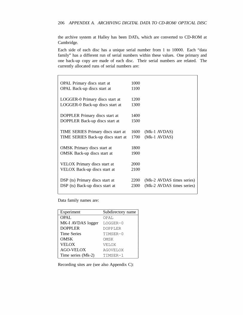
206 APPENDIX A. ARCHIVING DIGITAL DATA TO CD-ROM/ OPTICAL DISC
the archive system at Halley has been DATs, which are converted to CD-ROM atCambridge.
Each side of each disc has a unique serial number from 1 to 10000. Each “datafamily” has a different run of serial numbers within these values. One primary andone back-up copy are made of each disc. Their serial numbers are related. Thecurrently allocated runs of serial numbers are:
OPAL Primary discs start at 1000OPAL Back-up discs start at 1100
LOGGER-0 Primary discs start at 1200LOGGER-0 Back-up discs start at 1300
DOPPLER Primary discs start at 1400DOPPLER Back-up discs start at 1500
TIME SERIES Primary discs start at 1600 (Mk-1 AVDAS)TIME SERIES Back-up discs start at 1700 (Mk-1 AVDAS)
OMSK Primary discs start at 1800OMSK Back-up discs start at 1900
VELOX Primary discs start at 2000VELOX Back-up discs start at 2100
DSP (ts) Primary discs start at 2200 (Mk-2 AVDAS times series)DSP (ts) Back-up discs start at 2300 (Mk-2 AVDAS times series)
Data family names are:
Experiment Subdirectory nameOPAL OPALMK-I AVDAS l ogger LOGGER-0DOPPLER DOPPLERTime Series TIMSER-0OMSK OMSKVELOX VELOXAGO-VELOX AGOVELOXTime series (Mk-2) TIMSER-1
Recording sites are (see also Appendix C):
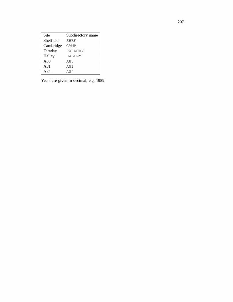
207
Site Subdirectory nameSheffield SHEFCambridge CAMBFaraday FARADAYHalley HALLEYA80 A80A81 A81A84 A84
Years are given in decimal, e.g. 1989.

Appendix B
Acronyms
ADC Analogue to Digital ConverterAGC Automatic Gain ControlAGO Automatic Geophysical ObservatoryAIS Advanced Ionospheric SounderAMPTE Active Magnetospheric Particle Tracer ExplorersASG Auroral Studies GroupAVDAS Advanced VLF Data Analysis SystemBAS British Antarctic SurveyBCD Binary Coded DecimalCCS Compressed Cross Spectrum (file type)CDF Common Data FormatCDHF Central Data Handling FacilityCD-ROM Compact Disc - Read Only MemoryCPS Compressed auto (Power) Spectrum (file type)CPU Central Processor UnitCSA Complex Spectral Amplitude (file type)CWO Clockwork Orange (receiver hut)DAT Digital Audio TapeDE-1 Dynamics Explorer 1 (satellite)DOS Disc Operating SystemDSP Digital Signal ProcessingELBBO Extended Life Balloon borne ObservatoryELF Extremely Low Frequency (30 Hz – 3 kHz)FET Field Effect TransistorFFT Fast Fourier TransformFHL Fast High/Low (OMSK file)FIFO First In First Out (buffer)FSD Full Scale DeviationFSK Frequency Shift KeyingGDS Geophysical Data SystemGGS Global Geospace Study
208
209
GIF Graphical Interchange FormatGPG Geospace Plasma GroupGPS Global Positioning SystemHPGL Hewlett Packard Graphics LanguageHGA High Greave Associates, SheffieldIGY International Geophysical Year (1957–58)IMS International Magnetospheric Study (1977–1979)ips inches per secondIRIS Imaging RIometer SystemISAAC International South Atlantic Anomaly Campaign (1983)ISTP International Solar Terrestrial Physics ProgrammeLAN Local Area NetworkLSB Least Significant ByteMCR Multi-channel ReceiverMLR Magnetospheric Line RadiationMLT Magnetic Local TimeMSB Most Significant ByteMS-DOS Microsoft Disc Operating SystemMSK Minimum Shift KeyingNERC Natural Environment Research CouncilOmniPAL Omni- Phase and Amplitude LoggerOMSK Omega and MSKOPAL Omega Phase and Amplitude LoggerORE Omega Reference EpochPROMIS Polar Regions and Magnetosphere International StudyPC (IBM PC/XT/AT-compatible) Personal ComputerQP Quasi-periodic (emissions)RALF Real-time Antarctic Logger Facility (ULF/VLF experiment)rms root mean squareRSEG Research Systems Engineering Group (responsible for UASD data)RVM Rubidium Vapour MagnetometerRx ReceiverSAS Signal Analyzer and Sampler (Hungarian VLF instrument on the ACTIVE satellite)SEAL Sheffield ELF/VLF Automatic LaboratorySHL Slow High/Low (OMSK file)SSB Space Sciences Building (at Halley)TCG Time Code GeneratorTCGR Time Code Generator/ ReaderUASD Upper Atmospheric Sciences Division (of BAS)ULF Ultra Low Frequency (below 30 Hz)VELOX VLF-ELF Logger ExperimentVDU Video Display UnitVLF Very Low Frequency (3–30 kHz)VU VELOX UnitsWIPP Wave-Induced Particle Precipitation (Campaign) 1987
210 APPENDIX B. ACRONYMS
WM Whistler ModeWORM Write Once, Read Many timeswrt with respect to
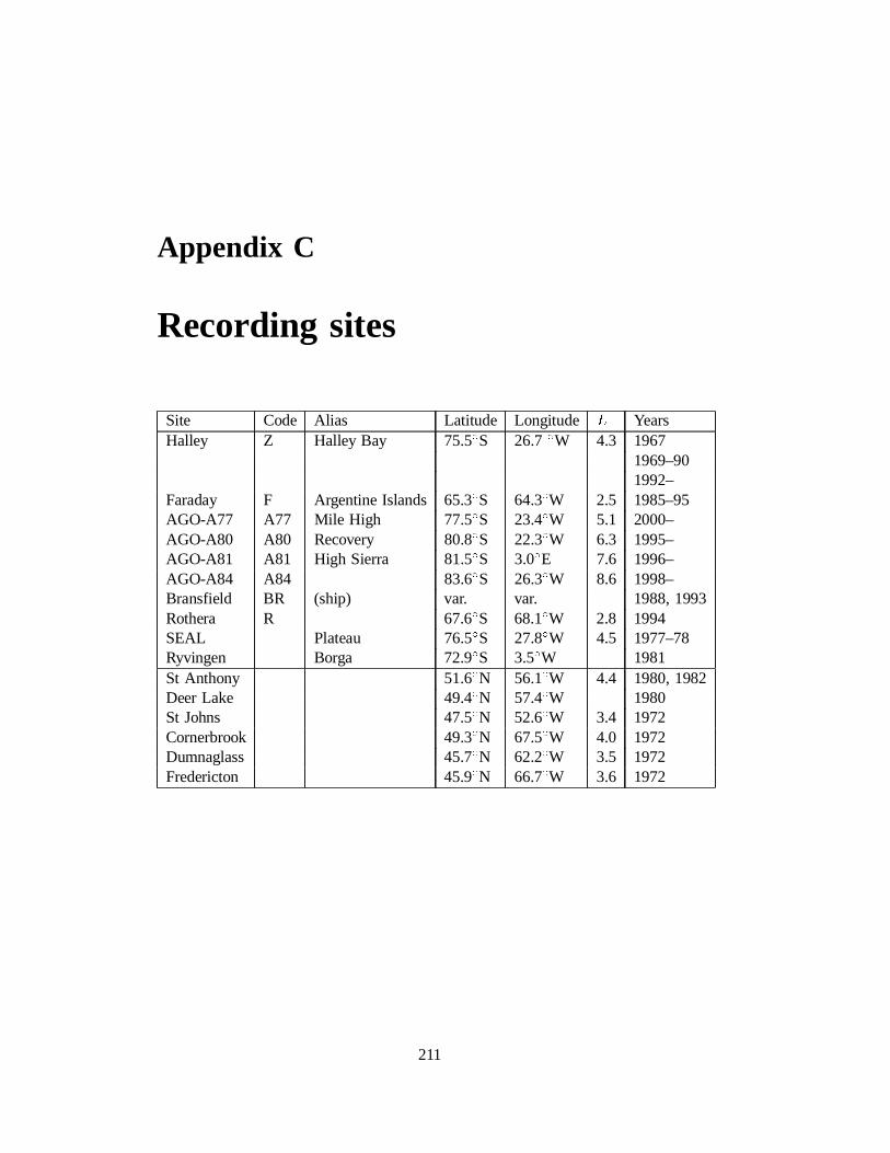
Appendix C
Recording sites
Site Code Alias Latitude LongitudeL Years± ±Halley Z Halley Bay 75.5 S 26.7 W 4.3 1967
1969–901992–
± ±Faraday F Argentine Islands 65.3 S 64.3 W 2.5 1985–95± ±AGO-A77 A77 Mile High 77.5 S 23.4 W 5.1 2000–± ±AGO-A80 A80 Recovery 80.8 S 22.3 W 6.3 1995–± ±AGO-A81 A81 High Sierra 81.5 S 3.0 E 7.6 1996–± ±AGO-A84 A84 83.6 S 26.3 W 8.6 1998–
Bransfield BR (ship) var. var. 1988, 1993± ±Rothera R 67.6 S 68.1 W 2.8 1994± ±SEAL Plateau 76.5 S 27.8 W 4.5 1977–78± ±Ryvingen Borga 72.9 S 3.5 W 1981± ±St Anthony 51.6 N 56.1 W 4.4 1980, 1982± ±Deer Lake 49.4 N 57.4 W 1980± ±St Johns 47.5 N 52.6 W 3.4 1972± ±Cornerbrook 49.3 N 67.5 W 4.0 1972± ±Dumnaglass 45.7 N 62.2 W 3.5 1972± ±Fredericton 45.9 N 66.7 W 3.6 1972
211

Appendix D
Transmitter information
D.1 Navigational transmitters
Omega was a global VLF radio navigational system. It was switched off perma-nently on 30 September 1997. There were eight widely distributed transmitters. Thetransmissions were accurately phase stable and a position fix could be obtained bymeasuring the relative phases of signals received from different transmitters. Thetransmission format is given in the table below.
D.1.1 Omega format
Segment A B C D E F G H ADuration (s) 0.9 1.0 1.1 1.2 1.1 0.9 1.2 1.0 0.9Start (s) 0.0 1.1 2.3 3.6 5.0 6.3 7.4 8.8 10.0
1Norway 10.2 13.6 11 12.1 12.1 11.05 12.1 12.1 10.23
1Liberia 12.0 10.2 13.6 11 12.0 12.0 11.05 12.0 12.03
1Hawaii 11.8 11.8 10.2 13.6 11 11.8 11.8 11.05 11.83
1N Dakota 11.05 13.1 13.1 10.2 13.6 11 13.1 13.1 11.053
1Reunion 12.3 11.05 12.3 12.3 10.2 13.6 11 12.3 12.33
1Argentina 12.9 12.9 11.05 12.9 12.9 10.2 13.6 11 12.93
1 1Australia 11 13.0 13.0 11.05 13.0 13.0 10.2 13.6 113 3
1Japan 13.6 11 12.8 12.8 11.05 12.8 12.8 10.2 13.63
Notes:
1. Omega transmissions were broadcast in a 10 s long cyclic format consisting of8 segments labelled A to H (first row of table).
2. The segments had different durations between 0.9 s and 1.2 s, separated by agap of 0.2 s (second row of table).
3. The times of the start of the segments were relative to the start of segment A,which was known as the Omega Reference Epoch (ORE) (third row of table).
212
D.1. NAVIGATIONAL TRANSMITTERS 213
4. The ORE was synchronised to an exact second of UT. However it was lockedto atomic time and could change by a whole second, relative to UTC, if a leapsecond was added or subtracted. This may happen at midnight on 30 Juneor 31 December each year. See table below for a chronological list of OREchanges.
5. In each segment, each of the eight Omega stations broadcast a signal at afrequency which was either one of the four common frequencies (10.2, 11.05,11.33, 13.6 kHz) or a frequency which was unique to that station (fourth andsubsequent rows of the table). All the frequencies were highly stable (ontransmission) since they were locked to atomic time.
6. The Omega format was such that each station transmitted each of the commonfrequencies once and its unique frequency four times in every cycle. In eachsegment, each of the four common frequencies was being transmitted by oneand only one station.
7. The Omega transmitters had a nominal radiated power of 10 kW.
8. The stations were operated by the US Naval Observatory, which publishedregular bulletins about their operation; these provided (usually after the event)information about when the stations were off the air, or were operating atreduced power.
9. A similar system, known as Alpha, is or was operated by the Soviet Navy usingtransmitters located in the (former) USSR. The frequencies used are approxi-mately 11.905, 12.649, and 14.881 kHz; they are in the ratio 16:17:20. Theformat consists of 0.4 s pulses in a 3.6 s cycle. Three 50 kW transmitters are
± ± ± ±used, located at Krasnodar (45.0 N; 38.0 E), Novosibirsk (55.1 N; 83.0 E),± ±and Komsomolsk (50.6 N; 137.0 E).
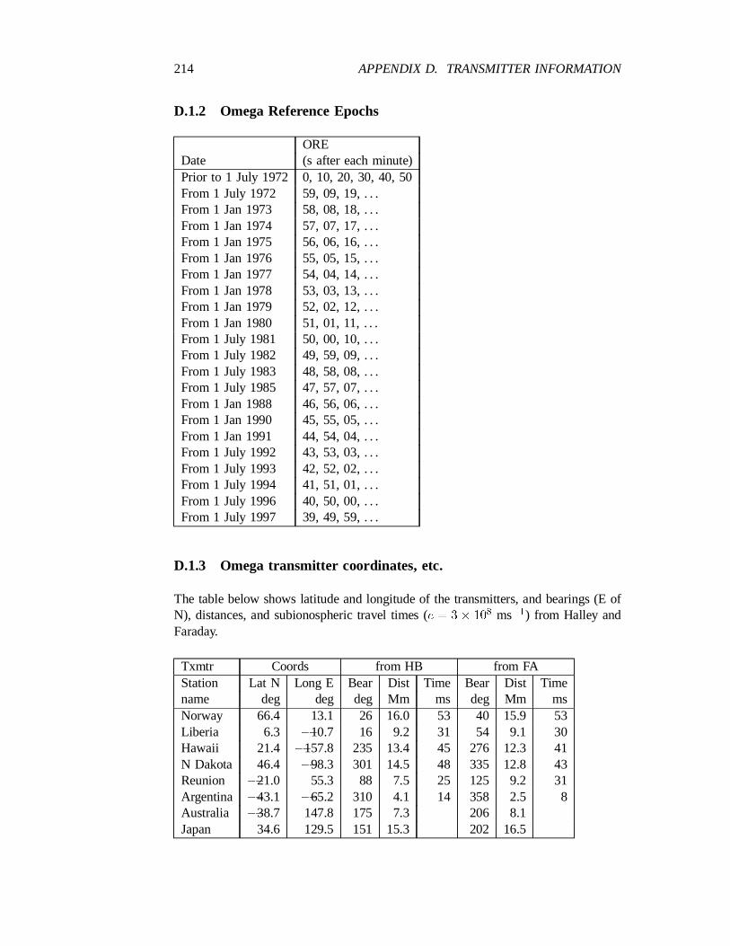
214 APPENDIX D. TRANSMITTER INFORMATION
D.1.2 Omega Reference Epochs
OREDate (s after each minute)Prior to 1 July 1972 0, 10, 20, 30, 40, 50From 1 July 1972 59, 09, 19, . . .From 1 Jan 1973 58, 08, 18, . . .From 1 Jan 1974 57, 07, 17, . . .From 1 Jan 1975 56, 06, 16, . . .From 1 Jan 1976 55, 05, 15, . . .From 1 Jan 1977 54, 04, 14, . . .From 1 Jan 1978 53, 03, 13, . . .From 1 Jan 1979 52, 02, 12, . . .From 1 Jan 1980 51, 01, 11, . . .From 1 July 1981 50, 00, 10, . . .From 1 July 1982 49, 59, 09, . . .From 1 July 1983 48, 58, 08, . . .From 1 July 1985 47, 57, 07, . . .From 1 Jan 1988 46, 56, 06, . . .From 1 Jan 1990 45, 55, 05, . . .From 1 Jan 1991 44, 54, 04, . . .From 1 July 1992 43, 53, 03, . . .From 1 July 1993 42, 52, 02, . . .From 1 July 1994 41, 51, 01, . . .From 1 July 1996 40, 50, 00, . . .From 1 July 1997 39, 49, 59, . . .
D.1.3 Omega transmitter coordinates, etc.
The table below shows latitude and longitude of the transmitters, and bearings (E of8 ¡1N), distances, and subionospheric travel times (c = 3£ 10 ms ) from Halley and
Faraday.
Txmtr Coords from HB from FAStation Lat N Long E Bear Dist Time Bear Dist Timename deg deg deg Mm ms deg Mm msNorway 66.4 13.1 26 16.0 53 40 15.9 53Liberia 6.3 ¡10.7 16 9.2 31 54 9.1 30Hawaii 21.4 ¡157.8 235 13.4 45 276 12.3 41N Dakota 46.4 ¡98.3 301 14.5 48 335 12.8 43Reunion ¡21.0 55.3 88 7.5 25 125 9.2 31Argentina ¡43.1 ¡65.2 310 4.1 14 358 2.5 8Australia ¡38.7 147.8 175 7.3 206 8.1Japan 34.6 129.5 151 15.3 202 16.5
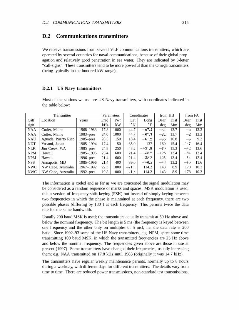
D.2. COMMUNICATIONS TRANSMITTERS 215
D.2 Communications transmitters
We receive transmissions from several VLF communications transmitters, which areoperated by several countries for naval communications, because of their global prop-agation and relatively good penetration in sea water. They are indicated by 3-letter“call-signs”. These transmitters tend to be more powerful than the Omega transmitters(being typically in the hundred kW range).
D.2.1 US Navy transmitters
Most of the stations we use are US Navy transmitters, with coordinates indicated inthe table below:
Transmitter Parameters Coordinates from HB from FACall Location Years Freq Pwr Lat Long Bear Dist Bear Dist
± ±sign kHz kW N E deg Mm deg MmNAA Cutler, Maine 1968–1983 17.8 1000 44.7 ¡67:3 ¡34 13.7 ¡2 12.2NAA Cutler, Maine 1983–pres 24.0 1000 44.7 ¡67:3 ¡34 13.7 ¡2 12.2NAU Aguada, Puerto Rico 1985–pres 28.5 150 18.4¡67:2 ¡38 10.8 ¡3 9.3NDT Yosami, Japan 1985–1994 17.4 50 35.0 137 160 15.4¡147 16.4NLK Jim Creek, WA 1985–pres 24.8 250 48.2¡121:9 ¡79 15.3 ¡42 13.6NPM Hawaii 1985–1996 23.4 600 21.4¡158:2 ¡126 13.4 ¡84 12.4NPM Hawaii 1996–pres 21.4 600 21.4¡158:2 ¡126 13.4 ¡84 12.4NSS Annapolis, MD 1985–1996 21.4 400 39.0¡76:5 ¡43 13.2 ¡10 11.6NWC NW Cape, Australia 1967–1992 22.3 1000¡21:8 114.2 143 8.9 178 10.3NWC NW Cape, Australia 1992–pres 19.8 1000¡21:8 114.2 143 8.9 178 10.3
The information is coded and as far as we are concerned the signal modulation maybe considered as a random sequence of marks and spaces. MSK modulation is used;this a version of frequency shift keying (FSK) but instead of simply keying betweentwo frequencies in which the phase is maintained at each frequency, there are two
±possible phases (differing by 180 ) at each frequency. This permits twice the datarate for the same bandwidth.
Usually 200 baud MSK is used; the transmitters actually transmit at 50 Hz above andbelow the nominal frequency. The bit length is 5 ms (the frequency is keyed betweenone frequency and the other only on multiples of 5 ms); i.e. the data rate is 200baud. Since 1992–93 some of the US Navy transmitters, e.g. NPM, spent some timetransmitting 100 baud MSK, in which the transmitted frequencies are 25 Hz aboveand below the nominal frequency. The frequencies given above are those in use atpresent (1997). Some transmitters have changed their frequencies, usually increasingthem; e.g. NAA transmitted on 17.8 kHz until 1983 (originally it was 14.7 kHz).
The transmitters have regular weekly maintenance periods, normally up to 8 hoursduring a weekday, with different days for different transmitters. The details vary fromtime to time. There are reduced power transmissions, non-standard test transmissions,
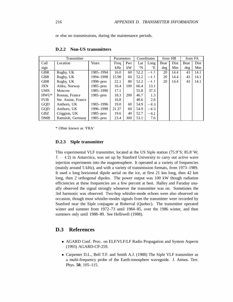
216 APPENDIX D. TRANSMITTER INFORMATION
or else no transmissions, during the maintenance periods.
D.2.2 Non-US transmitters
Transmitter Parameters Coordinates from HB from FACall Location Years Freq Pwr Lat Long Bear Dist Bear Dist
± ±sign kHz kW N E deg Mm deg MmGBR Rugby, UK 1985–1994 16.0 60 52.2¡1:1 20 14.4 43 14.1GBR Rugby, UK 1994–1998 15.98 60 52.2¡1:1 20 14.4 43 14.1GBR Rugby, UK 1998–pres 22.1 80 52.2¡1:1 20 14.4 43 14.1JXN Aldra, Norway 1985–pres 16.4 100 66.4 13.1UMS Moscow 1985–1990 17.1 55.8 37.3HWU* Rosnay, France 1985–pres 18.3 200 46.7 1.3FUB Ste. Assise, France 16.8 48.6 2.6GQD Anthorn, UK 1985–1996 19.0 60 54.9¡3:3
GQD Anthorn, UK 1996–1998 21.37 60 54.9¡3:3
GBZ Criggion, UK 1985–pres 19.6 40 52.7¡3:1
DMB Ramsloh, Germany 1985–pres 23.4 300 53.1 7.6
* Often known as ‘FRA’
D.2.3 Siple transmitter
± ±This experimental VLF transmitter, located at the US Siple station (75.9 S; 85.8 W;L = 4:2) in Antarctica, was set up by Stanford University to carry out active waveinjection experiments into the magnetosphere. It operated at a variety of frequencies(mainly around 5 kHz), and with a variety of transmission formats, from 1973–1989.It used a long horizontal dipole aerial on the ice, at first 21 km long, then 42 kmlong, then 2 orthogonal dipoles. The power output was 100 kW though radiationefficiencies at these frequencies are a few percent at best. Halley and Faraday usu-ally observed the signal strongly whenever the transmitter was on. Sometimes the3rd harmonic was observed. Two-hop whistler-mode echoes were also observed onoccasion, though most whistler-modes signals from the transmitter were recorded byStanford near the Siple conjugate at Roberval (Quebec). The transmitter operatedwinter and summer from 1972–73 until 1984–85, over the 1986 winter, and thensummers only until 1988–89. See Helliwell (1988).
D.3 References
² AGARD Conf. Proc. on ELF/VLF/LF Radio Propagation and System Aspects(1993) AGARD-CP-259.
² Carpenter D.L., Bell T.F. and Smith A.J. (1988) The Siple VLF transmitter asa multi-frequency probe of the Earth-ionosphere waveguide. J. Atmos. Terr.Phys.50, 105–115.

D.3. REFERENCES 217
² Cotton P.D., Smith A.J., Wolf T.G, Poulsen W.L., and Carpenter D.L. (1992)The propagation of mixed polarisation VLF (f ·5 kHz) radio waves in theAntarctic earth-ionosphere waveguide. Radio Sci.27, 593–610.
² Helliwell R.A. and Katsufrakis J.P. (1978) Controlled wave-particle interactionexperiments. inUpper Atmosphere Research in Antarcticaed. L.J. Lanzerottiand C.G. Park, American Geophysical Union.
² Helliwell R.A. (1988) VLF wave stimulation experiments in the magnetospherefrom Siple station, Antarctica. Rev. Geophys.26, 535-549.
² International Frequency List, International Telecommunications Union, Geneva.
² Swanson E.R. (1971) Omega. Navigation18, 168–175.
² Thomson N.R. (1981) Whistler mode signals: spectrographic group delays. J.Geophys. Res.86, 4795–4802.
² Thomson N.R. (1993) Experimental daytime VLF ionospheric parameters. J.Atmos. Terr. Phys.55, 173–184.
² USNO (1976) Worldwide Primary VLF and HF transmissions. US NavalObservatory Bulletin, Series 1, No. 3.
² US Naval Observatory Bulletins, Series 4 (give information on when transmit-ters were off the air). The paper reports finished in December 1996, but thesame information may be found on the Internet atftp://tycho.usno.navy.mil/pub/vlf/
Appendix E
Producing Graphics Plots
E.1 Introduction
For several of the data sets described in this manual, plots of the data are producedusing the PC-based AV-GRAF graphics system. This was created by Keith Yearbyand is fully described in separate documentation. It allows programmes to producegraphical output containing both line drawings and image data (e.g. spectrograms) ina form which may be displayed on the PC screen and plotted on a suitable hardcopydevice. The programmer’s interface to the system is a set of C functions whichallow lines, characters and image data to be either displayed directly on the screenor written to a file. The file, usually given a.GRF filename extension, may then beplotted to produce a hard copy or viewed on the PC screen. The C functions use afixed co-ordinate range to represent the area of the screen or paper no matter whichgraphics adapter the PC is fitted with or which hardcopy device is used.
To allow maximum compatibility with other graphics systems, the format chosen forthe graphics files for line drawing is a subset of HPGL (the industry standard graphicslanguage used by Hewlett Packard plotters). For image data a format known withinour group as “BBC/Diablo” is used with a header (in the style of HPGL) to describethe origin and pixel size. [This format was developed at BAS in the late 1980s forplotting files stored on an Acorn BBC computer to a Diablo C150 inkjet printer.]
Besides the graph plotting programmes detailed below, the system includesGENGRAPH,a general-purpose graph-plotting programme which will not be further described here.
E.2 Graphics adapters and plotting devices
At present the system will support the use of the following graphics adapters andplotting devices.
Graphics adapters: VGA (others could be used for quick look).
218

E.3. GRAPHICS FILE PLOTTING COMMANDS 219
Plotting devices: HP Paintjet printer, any PostScript printer, and output to GIF files
E.3 Graphics file plotting commands
The commandsVIEW (for PC screen),PLOTHPP(for HP PaintJet),PLOTPS(forPostScript) andPLOTGIF (for GIF format image files) are provided to plot graphicsfiles. The syntax is:
VIEW ¡graphics file name¿
or
PLOTHPP ¡graphics file name¿ ¡printer file name¿ [/m]COPY/B ¡printer file name¿ LPT1:
(assuming LPT1: is the Paintjet printer)
or
PLOTPS ¡graphics file name¿ ¡printer file name¿ [ /i /c ]COPY ¡printer file name¿ LPT2:
(assuming LPT2: is the PostScript printer)
or
PLOTGIF ¡graphics file name¿ ¡GIF file name¿ [ /m /r /t ]
TheVIEWcommand scans the graphics files and plots the contents on the PC screen.If image data are encountered they will be plotted properly only if the VGA mode isin use, although other modes will make an attempt to display them.
PLOTHPPscans the file and first plots the data into a pixel map of 640 by 480 pointsheld in memory (with 16 plotter units per point). When the end of the file is reached,the pixel map is dumped into the printer file. Each point in the pixel map is printedas a 3 by 3 square of printer dots. The printer resolution is 180 dots per inch whichgives an overall scale factor of 960 plotter units per inch. This gives a slightly largerplot than the HPGL standard of 1024 plotter units per inch. If the/m option is used,the plot is produced in monochrome instead of colour.
PLOTPSsimply translates the graphics commands in the input file to PostScript.The resulting output files are typically about four times as large as the input file. Ifthe /c option is specified, image data will be plotted using a colour palette ratherthan the default monochrome palette. If the/i option is used, the monochrome orcolour palette used for image data will be inverted (e.g. black appears white andvisa versa).PLOTPSversion 3 reads the PostScript pre-amble from a separate file,
220 APPENDIX E. PRODUCING GRAPHICS PLOTS
PLOTPS3.INI , which must be in the default directory or in the PATH. This filecould be modified by the user to change the colour palette.
PLOTGIF scans the file and first plots the data into a pixel map of 640 by 480points held in memory (with 16 plotter units per point). When the end of the fileis reached the pixel map is dumped into the GIF file. The three options control thebit map dump. If/m is specified, a monochrome palette will be used instead of thedefault colour palette. By defaultPLOTGIF assumes that the plot is orientated inlandscape mode;/r will cause the image to be rotated so that portrait mode plotswill be correctly orientated when the GIF file is viewed./t will trim off all whitespace from the top, bottom and sides of the image.
E.4 Batch file processing
Often it will be required to produce similar plots for a set of data files on disc orCD-ROM. Sometimes the Paintjet printer does not correctly exit its graphics modeafter plotting, and it is advisable to reset it between plots. Since the plotting takessome time, such jobs are often run overnight. A number of MS-DOS batch filesexist to achieve this. For exampleGPRINT printer-filename [/ff] executesthe COPY/B command, optionally advances the paper to the top of the next form,and resets the printer;AVPLOT graphics-filename [/m] executes both thePLOTHPP(with the optional/m specifying monochrome) andCOPY/B commands,formfeeds and resets the printer, and deletes the no longer required printer file. Plotsfrom a number of graphics files can be produced by executing a batch file of the type
CALL AVPLOT ¡graphics file name 1¿ [/m]CALL AVPLOT ¡graphics file name 2¿ [/m]....etc.
A similar batch fileAVPLOTPS.BATexists for producing multiple PostScript plots.
E.5 Documentation
² A graphics system for data analysis on IBM PC computers, K.H. Yearby, June1990 (revised Feb 1991, Oct 1992, Feb 1996).
² World Wide Web:http://www.acse.shef.ac.uk/˜keith/avgraf/manual.ht
Appendix F
List of Figures
Fig. 1.1 AVDAS colour spectrogram plot (Halley 1992 194:00:05:23 UT) printedon the HP Paintjet printer. See AVDAS manual for details. Thex-axis istime in seconds relative to the time shown at the top. They-axis is frequencyin Hz. The z-axis (colour scale) is intensity in dB (the 0 dB level can beestablished from the calibration tone). Spectrograms can alternatively be printedin monochrome (grey-scale).
Fig. 1.2 Similar to Fig. 1.1 (for Halley 1992 194:00:35:29 UT) but with the averagerenabled, giving a longer time interval on the plot (at the expense of timeresolution).
Fig. 1.3 Typical output fromQLOOK(for Halley 1992 day 182 00–12 UT) with astandard 1-minute-in-five sampling, 0–8 kHz spectrogram display. There is 12hours coverage on a page.
Fig. 2.1 Example of an AVDAS spectrogram of a frequency translated recording(Halley 1992 218:03:12:23 UT). N.B. in this particular case the frequencyappears to have been translated down by 13 kHz instead of the recommended15 kHz. Also the frequency offset function of AVDAS has not been used toprovide the correct frequency scale. Aliases of some Omega transmissions areseen.
Fig. 3.1 24-hr plot of AVDAS logger data (Halley, day 197, 1987).
Fig. 4.1 Trimpi data (Halley, day 256, 1986; from Toby Clark’s 1986 Halley VLFreport); NSS 21.4 kHz.
Fig. 5.1 Two component time series data, plotted withDSPPLOT(Halley, day 221,1989, 1653:37 UT).
Fig. 6.1 RALF data plot showing ULF-H (combination ofX and Y ) and VLF 1kHz channels; Halley 21 Sept 1986, 1012–1024 UT.
221
222 APPENDIX F. LIST OF FIGURES
Fig. 7.1 Plot of VLF Doppler data made usingPC-DPLOT; uncalibrated powerHXQ; Faraday NAA 21.4 kHz; start time 2130 UT 23 March 1993.
Fig. 7.2 Same as Fig. 7.1 but showing Doppler shift instead of power.
Fig. 7.3 Same as Fig. 7.1 but showing azimuth instead of power.
Fig. 8.1 OMSK data plotted usingOMSKSEQwith option FORM=2. Faraday; starttime 06:24:54 UT 7 April 1990. Showing Omega Argentina, Omega Hawaii(actually off the air at the time), NAA and NPM.
Fig. 8.2 OMSK data plotted usingOMSKSEQwith optionsFORM=1, STAT=2. Fara-day; NAA start time 06:24:54 UT 7 April 1990.
Fig. 8.3 OMSK data plotted usingOMSKSEQwith optionsFORM=1, FREQ=4, DIF=1 .Faraday; start time 06:24:54 UT 7 April 1990.
Fig. 8.4 OMSK data plotted usingOMSKSEQwith optionsFORM=1, FREQ=4, DIF=0 .Faraday; start time 06:24:54 UT 7 April 1990.
Fig. 8.5 OMSK data plotted usingOMSKVIEWwith optionOUT=001. Faraday; starttime 06:14:54 UT 7 April 1990.
Fig. 9.1 Example of a VELOX data plot produced byVLXPLOTshowing just thescalar data (/S option); Halley 1992, day 334, 00–10 UT. The command usedto generate this figure was:
VLXPLOT VLX92334.DAT /S /N=1 /O=VPLOT
This produced the fileVPLOT000.GRF which was then printed as describedin Appendix E. Since they were not specified, the following default valueshave been used:X=16, MAXAMP=70, MINAMP=10, and data are plotted fromthe beginning of the file. As this 1992 file contains only phase 1 data, it is notnecessary to specify/1 or /2 .
Fig. 9.2 Example of a VELOX data plot produced byVLXPLOTshowing the scalar,minimum and peak data (/S/M/P options); Halley 1992, day 315, 00–01 UT.Command:
VLXPLOT VLX92315.DAT /S /M /P /X=160 /N=1 /O=VPLOT
Fig. 9.3 Example of a VELOX data plot produced byVLXPLOTshowing the scalar,azimuth and ellipticity data (/S/A/E options); Halley 1992, day 315, 00–01 UT. Command:
VLXPLOT VLX92315.DAT /E /A /X=160 /N=1 /O=VPLOT
Fig. 9.4 Example of a VELOX data plot produced byVLXSPEC; Halley 1992, day315. Command:
223
VLXSPEC VLX92315.DAT /X=12 /O=VSPEC
As none of/S, /M, /P, /E, /A were specified, the default (/S ) was used.A value of 16 for X, rather than the default of 12, plots 24 hours on a frame.
Fig. 9.5 Example of a phase 2 VELOX data plot produced byVLXPLOTshowingnarrow-band and impulse data (/2/S/I options); Halley 1997, day 119, 00–10 UT. Command:
VLXPLOT VLX97119.DAT /2 /S /I /N=1 /V /O=VPLOT
In this case the averaging/V option has been used to produced a smootherplot.
Fig. 10.1 Example of mode A AGO-VELOX data, in this case A80, day 122 (1May) 1996. The data are plotted using theVLXSPECprogramme. The threeout of 8 standard VELOX bands which are not recorded by AGO-VELOX areclearly visible as horizontal black bands. The command to produce this plotwas:
VLXSPEC VA196122.DAT /X=12 /O=VSPEC
Fig. 10.2 Example of a record of mode B AGO-VELOX data, in this case the1205 UT record from A80 on day 122 (1 May) 1996. The data are plot-ted using theAGOSPECprogramme. The daily calibration signal appears onthis plot; the command for it was:
AGOSPEC AS196122.DAT /D=122 /T=1205 /N=1 /O=ASPEC
which produced the AV-GRAF format fileASPEC000.GRF.
Fig. 10.3 Example of 12 hours of mode B AGO-VELOX data, from A80 on day122 (1 May) 1996, plotted in quicklook format byAGOQLK. The commandwas simply:
AGOQLK AS196122.DAT
which produced two AV-GRAF format files,AQ12200.GRF andAQ12212.GRF.The former is shown here. The quicklook plots tend to look better in monochromethan colour, so the/m option is normally used when producing the plots (e.g.by PLOTPS).
Appendix G
Index
224
Index
10 kHz pilot tone, 18, 44 CALPROC, 35AbsPAL, 148 Catalogue format, 30Acronyms, 210 CATLOG, 56Adams, Kit, 156 CCS files, 91, 94ADC Units, 123 CHECKLG, 54, 57ADIOS-II card, 124 Chronos, 149Aerials, 14 Clark, Toby, 18AGO-VELOX data, 190 CONVFTOS, 162AGO-VELOX file formats, 193 Correlation coefficients, 132AGO2VLX, 198 CPS files, 92, 94AGOQLK, 203 CSA files, 91, 94AGOs, 171, 190 DAT recordings, 18AGOSORT, 200 DOPCAT, 142AGOSPEC, 202 DOPINT, 138Alpha transmitters, 215 DOPLOG, 136AnalyseFHL, 166 Doppler data files, 121AnalyseSHL, 166 DOPSCAN, 141Apple Macintosh, 124 DSP programme, 81Archiving digital data, 207 DSP-II, 33, 171ARCSERVE, 172 DSP3CP, 87Ariel-4 satellite, 52 DSP3SPEC, 89AV-GRAF graphics system, 220 DSPCAT, 85AV format, 153 DSPCOM, 71AVDAS, 32, 73 DSPPLOT, 77, 85AVDAS logger data, 51 DYLIST, 143AVDAS times series data, 69 Faraday configuration, 17AVDAS.CAL, 59 FHL format, 153AVDAS.NUL, 59 FIFO buffer, 196AVPLOT.BAT, 222 Film spectrograms strips, 39AVPLOTPS.BAT, 222 General Purpose Interface, 70AVT, 73 GGS key parameter files, 171Azimuth reference signal, 18 GIF image files, 221, 222BAS micro, 52, 75 Goniometer, 15BBC/Diablo format, 220 GPRINT.BAT, 222Broadband VLF receiver, 13 Graphical output, 220Calibration, 23 GRF filename extension, 220Calibration tones, 178 High Greave Associates, 15, 33, 44,
225
226 INDEX
Index171 PINFO-A.TXT, 58
HPGL, 222 PLOTGIF, 221, 222HS format, 152, 153 PLOTHPP, 221ID array, 130 PLOTLOG, 57Input Means, 131 PLOTPS, 221, 222IRIG-B time code, 171 PLOTPS3.INI, 222Jones, Dyfrig, 69 PostScript, 222Kressmann, Dick, 195 PostScript printer, 35, 203, 221Log books, 27 Preamplifiers, 15, 122Log file format, 28 Princeton TRA-50 frequency transla-
tor, 44LOGCAT, 27QLOOK, 35LSRCACHE, 207Quick look system, 35MLRSCAN, 35Quicklook plots, 40Morrison, Keith, 111RALF analysis software, 113Multi-channel receiver, 52RALF data, 97NAADAT.FAR, 121RDLOGGER.PRO, 59NAADF, 126Recording sites, 213NAADFY, 127Results files, 39NAADIR.FAR, 121Revox tape recorders, 18, 33, 44Non-US transmitters, 218Robertson, John, 156Oldfield, Jon, 178RRS Bransfield, 129OLDNEW, 122Rules of the Road, 8Omega, 214RX50 format, 130OmniPAL receiver, 148Ryvingen, 19OMSK receiver, 147Saxton, John, 138OMSK.EXE, 148SEAL, 17, 19OMSKCAT, 159Sheffield University, 16, 52OMSKCOPY, 163SHL format, 153OMSKDET, 163SIMULATE, 89OMSKLIST, 160Siple transmitter, 69, 218OMSKSCAL, 165South Pole VLF beacon, 169OMSKSEQ, 162SPECAT, 35OMSKVIEW, 161Stanford University, 169OPAL receiver, 147Tape playing times, 22OPAL.EXE, 148Tape speeds, 21OPALSEQ, 158TAPESF, 35Optical WORM discs, 207TBASEPC, 149Otago University, 121Thomson, Neil, 121PaintJet printer, 35, 82, 138, 203, 221,
222 Time code, 26Panasonic SV-3700, 33 Time marks, 24Paper chart records, 7 Translated frequency data, 43PC-DPLOT, 137 Transmitter details, 214Piggott Building, 17 TSAVE, 74
INDEX 227
Uher tape recorder, 18US Navy transmitters, 217VELOX data, 51, 169VELOX file formats, 172VELOXFIX, 178VIEW, 221VLFCHECK, 195VLXCDROM.TXT, 188VLXCOPY, 184VLXLIST, 180VLXLOG, 171VLXPLOT, 183VLXSPEC, 186WMDF2*, 128WMscrnTst, 124World-Wide Web, 7Year 2000, 7Yearby, Keith, 156, 220