barycentric discriminant analysis

B

Barycentric Discriminant Analysis

Hervé Abdi1, Lynne J. Williams2 andMichel Béra31School of Behavioral and Brain Sciences, TheUniversity of Texas at Dallas, Richardson,TX, USA2BC Children’s Hospital MRI Research Facility,Vancouver, BC, Canada3Centre d’Étude et de Recherche en Informatiqueet Communications, Conservatoire National desArts et Métiers, Paris, France

Synonyms

Intraclass analysis; Mean-centered partial leastsquare correlation

Glossary

Barycenter The mean of the observationsfrom a given category (alsocalled center of gravity, centerof mass, mean vector, orcentroid)

Confidenceinterval

An interval encompassing agiven proportion (e.g., 95%)of an estimate of a parameter(e.g., a mean)

Discriminantanalysis

A technique whose goal is toassign observations to somepredetermined categories

Discriminantfactor scores

A linear combination of thevariables of a data matrix. Usedto assign observations tocategories

Designmatrix (akagroup matrix)

In a group matrix, the rowsrepresent observations and thecolumns represent a set ofexclusive groups (i.e., anobservation belongs to one andonly one group). A value of 1 atthe intersection of a row and acolumn indicates that theobservation represented by therow belongs to the grouprepresented by the column.Avalue of 0 at the intersection ofa row and a column indicates thatthe observation represented bythe row does not belong to thegroup represented by the column

Estimationbias

The difference between thecomputed value of a barycenterand the mean of the bootstrappedestimates of this barycenter

Fixed effectmodel

Analysis in which theobservations that are predictedwere used to compute thepredictive model

# Springer Science+Business Media LLC 2018R. Alhajj, J. Rokne (eds.), Encyclopedia of Social Network Analysis and Mining,https://doi.org/10.1007/978-1-4614-7163-9_110192-2

https://doi.org/10.1007/978-1-4614-7163-9_110192-2

Inertia Aweighted sum of squareddistances of a set of points to agiven point (often the barycenterof the points). The concept ofinertia generalizes the concept ofthe variance of a set of points.

Learning set The observations that are used tocompute the predictive model

MultiblockBarycentricAnalysis

Also called multitable ormultiple subjects barycentricanalysis. A barycentric analysisin which the data table is madeof a concatenation of subdata-tables. Acronyms areMUBADA, MUSUBADA, andMUDICA

Predictioninterval

An interval encompassing agiven proportion (e.g., 95%) ofthe predicted observations froma given category

Randomeffect model

Analysis in which theobservations that are predictedwere not used to compute thepredictive model

Testing set A set of observations that werenot used to compute thepredictive model but are usedto evaluate the quality of theprediction

Toleranceinterval

An interval encompassing agiven proportion (e.g., 95%) ofthe observations from a givencategory

Definition

Barycentric discriminant analysis (BADA) is arobust version of discriminant analysis that isused to assign, to predefined groups (also calledcategories), observations described by multiplevariables. By contrast with traditional discrimi-nant analysis, BADA can be used even when thenumber of observations is smaller than the num-ber of variables – this makes BADA particularlysuited for the analysis of Big Data.

Introduction

Barycentric discriminant analysis (BADA (Abdi2007a; Bastin et al. 1982; Abdi and Williams2010c; Bergougnan and Couraud 1982; Beatonet al. 2014)) is a robust version of discriminantanalysis that is used – like discriminant analysis(Abdi 2003) – when multiple measurementsdescribe a set of observations in which each obser-vation belongs to one category (i.e., group) from aset of a priori defined categories. The goal ofBADA is to combine the measurements to createnew variables (called components or discriminantvariables) that best separate the categories. Thesediscriminant variables are also used to assign theoriginal observations or “new” observations to thea-priori defined categories.

For example, BADA can be used (1) to assignsubjects to a given diagnostic group (i.e.,Alzheimer’s disease, other dementia, normalaging (Abdi et al. 2012a)) on the basis on brainimaging data or psychological tests (here thea-priori categories are the clinical groups), (2) toassign wines to a region of production on the basisof several physical and chemical measurements(here the a-priori categories are the regions ofproduction (Abdi 2007b)), (3) to use brain scanstaken on a given participant to determine whattype of object (e.g., a face, a cat, a chair) waswatched by the participant when the scans weretaken (here the a-priori categories are the types ofobject (Abdi et al. 2012b; St. Laurent et al. 2011)),(4) to use DNA measurements to predict if aperson is at risk for a given health problem (herethe a-priori categories are the types of healthproblem (El Behi et al. 2017; Cioli et al. 2014)).BADA is a very general discriminant techniquethat can also be used in cases for which standarddiscriminant analysis cannot be used. This isthe case, for example, when there are more vari-ables than observations (a case often called the“N << P problem”) or when the measurementsare qualitative (instead of quantitative as requiredby standard discriminant analysis).

2 Barycentric Discriminant Analysis

Key Points

Barycentric discriminant analysis is a robust ver-sion of discriminant analysis that is used when multiple measurements describe a set of observa-tions in which each observation belongs to one category (i.e., group) from a set of a priori defined categories. BADA combines the original vari-ables to create new variables that best separate the groups and that can also be used to optimally assign old or new observations to these categories. The quality of the performance is evaluated by cross-validation techniques that estimate the per-formance of the classification model for new observations.

BADA is a very versatile technique that can be declined in several different varieties that can handle, for example, qualitative data and data structured in blocks. This versatility makes BADA particularly suited for the analysis of mul-timodal and Big data.

Historical Background

BADA can be seen as a particular version of the two-table method of Tucker’s interbattery analy-sis (Tucker 1958) – a technique developed in the 1950s as a robust version of canonical correlation analysis. BADA, however, was first developed as such in the 1970s by the French school of data analysis (Benzécri 1977; Nakache et al. 1977; Leclerc 1976) for the specific case of classifying qualitative data (under the name of discriminant correspondence analysis). Subsequent develop-ments occurred within the framework of co-inertia analysis (an approach generalizing Tucker’s method that is particularly popular in Ecological studies, see Doledec and Chessel 1994) and also within the framework of partial least square correlation methods (another approach generalizing Tucker’s method that is particularly popular in brain imaging and genetic studies, see Krishnan et al. 2010).

Barycentric Discriminant Analysis(BADA)

BADA is, in fact, a class of methods which all relyon the same principle: Each category of interest isrepresented by the barycenter of its observations(i.e., the weighted average; the barycenter is alsocalled the center of gravity of the observations of agiven category), and a generalized principal compo-nent analysis (GPCA) is performed on the categoryby variable matrix. This analysis gives a set ofdiscriminant factor scores for the categories andanother set of factor scores for the variables. Theoriginal observations are then projected onto thecategory factor space, and this operation provides aset of factor scores for the observations. The dis-tance of each observation to all the categories iscomputed from the factor scores and each observa-tion is assigned to its closest category. The compar-ison between the a-priori and a-posteriori categoryassignments is used to assess the quality of thediscriminant procedure. The prediction for theobservations which were used to compute thebarycenters is called the fixed effect prediction.Fixed effect performance is evaluated by countingthe number of correct and incorrect assignments andstoring these numbers in a confusion matrix.Another index of the performance of the fixed effectmodel – equivalent to a squared coefficient ofcorrelation – is the ratio

R2 ¼ category variance

category variance þ variance of the:

observations

within category

(1)

This coefficient R2 is interpreted as the propor-tion of variance of the observations explained by thecategories or as the proportion of the varianceexplained by the discriminant model. The perfor-mance of the fixed effect model can also berepresented graphically as a tolerance ellipsoid thatencompasses a given proportion (say 95%) of theobservations. The overlap between the tolerance

Barycentric Discriminant Analysis 3

ellipsoids of two categories is roughly proportionalto the number of misclassifications between thesetwo categories.

New observations can also be projected ontothe discriminant factor space, and they can beassigned to the closest category. When the actualassignment of these observations is not known,the model can be used to predict category mem-bership. The model is then called a random effectmodel (as opposed to the fixed effect model). Anobvious problem, then, is to evaluate the qualityof the prediction for new observations. Ideally, theperformance of the random effect model is evalu-ated by counting the number of correct and incor-rect classifications for new observations andcomputing a confusion matrix on these new obser-vations. However, it is not always practical oreven feasible to obtain new observations, andtherefore the random effect performance is, ingeneral, evaluated using computational cross-validation techniques such as the jackknife (Abdiand Williams 2010a) or the bootstrap (Efron andTibshirani 1993). For example, a jackknifeapproach (also, better called, “leave one out”LOO) can be used by which each observation istaken out of the set, in turn, and predicted from themodel built on all the other observations. Thepredicted observations are then projected ontothe space of the fixed effect discriminant scores.The quality of the LOO prediction can also berepresented graphically as a prediction ellipsoid.A prediction ellipsoid encompasses a given pro-portion (say 95%) of the new observations. Theoverlap between the prediction ellipsoids of twocategories is roughly proportional to the numberof misclassifications of new observations betweenthese two categories.

The stability of the discriminant model can beassessed by a cross-validation model such as thebootstrap (Efron and Tibshirani 1993; Diaconisand Efron 1983). In this procedure, multiple setsof observations (called “Bootstrapped samples”)are generated by sampling with replacement fromthe original set of observations and the categorybarycenters are computed from each of these sets.

These barycenters are then projected onto thediscriminant factor scores. The variability of thebarycenters can be represented graphically as aconfidence ellipsoid that encompasses a givenproportion (say 95%) of the barycenters. Whenthe confidence intervals of two categories do notoverlap, this indicates that these two categoriesare significantly different.

In summary, BADA is a GPCA performed onthe category barycenters. Recall that GPCAencompasses different techniques such as,for example, correspondence analysis, biplot,Hellinger distance analysis, discriminant analysis,and canonical variate analysis (Abdi 2007a;Gittins 1980; Greenacre 1984). For each specifictype of GPCA, we have a corresponding versionof BADA. For example, when the GPCA used iscorrespondence analysis, this gives the most well-known version of BADA: discriminant corre-spondence analysis (DICA, also called correspon-dence discriminant analysis, see, e.g., Abdi2007b, Celeux and Nakache 1994, Leclerc 1976,Saporta and Niang 2006, Bastin et al. 1982,Bergougnan and Couraud 1982, Doledec andChessel 1994).

Notations

The original data matrix is an I observations byJ variables matrix denotedX. Prior to the analysis,the matrix X can be preprocessed by centering(i.e., subtracting the column mean from each col-umn), by transforming each column into aZ-score, or even by normalizing each row suchthat the sum of its elements or the sum of itssquared elements is equal to one. The observa-tions inX are partitioned intoN a-priori categoriesof interest, with In being the number of observa-

tions of the nth category (and soPN

nIn ¼ I). The

general structure of the data matrix can be illus-trated as follows (note that for convenience, thenumbering of the rows is done within category):


Category 11 x1, 1 . . . x1, j . . . x1, J⋮ ⋮ ⋱ ⋮ ⋱ ⋮I1 xI1, 1 . . . xI1, j . . . xI1, J

8<

:

⋮

Category n1 x1, 1 . . . x1, j . . . x1, J⋮ ⋮ ⋱ ⋮ ⋱ ⋮In xIn, 1 . . . xIn, j . . . xIn, J

8<

:

⋮

Category N1 x1, 1 . . . x1, j . . . x1, J⋮ ⋮ ⋱ ⋮ ⋱ ⋮IN xIN, 1 . . . xIN, j . . . xIN, J

8<

:

(2)

Notations for the Categories (Rows)

We denote by Y the I by N design matrix (alsocalled a group matrix) for the categories (i.e.,groups) describing the rows of X : yi,n = 1 ifrow i belongs to category n, yi,n = 0 otherwise.We denote bym the I by 1 vector ofmasses for therows of X and by M the I by I diagonal matrixwhose diagonal elements are the elements of m(i.e., using the diag operator which transforms avector into a diagonal matrix, we have M = diag{m}). We denote by b the N by 1 vector of massesfor the categories describing the rows of X and byB the N by N diagonal matrix whose diagonalelements are the elements of b. Masses are posi-tive numbers; it is convenient (but not necessary)to have the sum of the masses equal to one.

Barycentric Discriminant Analysis:Computation

The first step of BADA is to compute thebarycenter of each of the N categories describingthe rows. The barycenter of a category is theweighted average of the rows where the weightsare the masses rescaled such that the sum of theweights for one category is equal to one. The N byJ matrix of barycenters is computed as

R ¼ diag Y⊺M1! "#1

Y⊺MX, (3)

where 1 is a conformable vector of 1s (the diago-nal matrix diag{YM1}#1 serves to rescale the

masses of the rows such that their sum is equalto one for each category).

Masses, Weights, and GPCA

The type of preprocessing of the data and thechoice of B (matrix of masses for the categories)and W (matrix of weights for the variables) iscrucial, because this choice determines the spe-cific type of GPCA used. For example, discrimi-nant correspondence analysis is obtained bytransforming the rows of R into relative frequen-cies, by using the relative frequencies of thebarycenters as their masses and by using theinverse of the column frequencies for the weightsof the variables. As another example, standarddiscriminant analysis is obtained when W isequal to the inverse of the within groupvariance-covariance matrix.

GPCA of the Barycenter MatrixThe R matrix is then analyzed using a GPCAunder the constraints provided by the matricesB (for the N categories) and W (for the columns).Specifically, the matrix R is analyzed with thegeneralized singular value decomposition (see,e.g., Abdi 2007a; Greenacre 1984) as

R ¼ PDQ⊺ with P⊺BP ¼ Q⊺WQ ¼ I, (4)

where D is the L by L diagonal matrix of thesingular values (with L being the number of non-zero singular values), and P (respectively Q)being the N by L (respectively J by L) matrix ofthe left (respectively right) generalized singularvectors of R.

Factor Scores

The N by L matrix of factor scores for the catego-ries is obtained as

F ¼ PD ¼ RWQ: (5)

The variance of the columns of F is given by


the square of the corresponding singular values(i.e., the “eigenvalue” denoted l; these are storedin the diagonal matrix L). This can be shown bycombining Eqs. 4 and 5 to give:

F⊺BF ¼ DP⊺BPD ¼ D2 ¼ L: (6)

The I rows of matrix X can be projected ontothe space defined by the factor scores of thebarycenters (this procedure is called a projectionas “supplementary,” or “illustrative,” or even“passive” elements; for more details see Abdiand Williams 2010b). Note that the matrix WQfrom Eq. 5 is a projection matrix. Therefore, theI by LmatrixH of the factor scores for the rows ofX can be computed as

H ¼ XWQ: (7)

These projections are barycentric, because theweighted average of the factor scores of the rowsof a category gives the factors scores of the cate-gory. This can be shown by first computing thebarycenters of the row factor scores as (cf. Eq. 3)as

H ¼ diag YM1f g#1 YMH, (8)

then plugging in Eq. 7 (see also Eq. 5) and devel-oping. Taking this into account, Eq. 8 becomes

H ¼ diag YM1f g#1 YMXWQ¼ RWQ ¼ F: (9)

Loadings

The loadings describe the variables of thebarycentric data matrix and are used to identifythe variables important for the separation betweenthe groups. As for standard PCA, there are severalways of defining the loadings. The loadings canbe defined as the correlation between the columnsof matrix R and the factor scores. Alternatively,the loadings can also be defined as the matrixQ or(as we did in our example), even, as

G ¼ QD: (10)

Quality of the Prediction

The performance, or quality of the prediction of adiscriminant analysis, is assessed by predictingthe category membership of the observations andby comparing the predicted with the actual cate-gory membership. The pattern of correct andincorrect classifications can be stored in a confu-sion matrix in which the columns represent theactual categories and the rows the predicted cate-gories. At the intersection of a row and a column isthe number of observations from the column cat-egory assigned to the row category.

The performance of the model can be assessedfor the observations used to compute the catego-ries: this is the fixed effect model. In addition, theperformance of the model can be estimated fornew observations (i.e., observations not used tocompute the model): This is the random effectmodel.

Fixed Effect: Old Observations

The fixed effect model predicts the categoryassignment for the observations that were usedto compute the barycenters of the categories. Inorder to assign an observation to a category, thefirst step is to compute the distance between thisobservation and all N categories. Then, the obser-vation is assigned to the closest category. Severalpossible distances can be chosen, but a naturalchoice is the Euclidean distance computed in thefactor space. If we denote by hi the vector of factorscores for the ith observation, and by fn the vectorof factor scores for the nth category, then thesquared Euclidean distance between the ith obser-vation and the nth category is computed as

d2 hi, fnð Þ ¼ hi # fnð Þ⊺ hi # fnð Þ: (11)

Obviously, other distances are possible (e.g.,Mahalanobis distance), but the Euclidean distancehas the advantage of being “directly read” onthe map.


Tolerance IntervalsThe quality of the category assignment of theactual observations can be displayed using toler-ance intervals (Abdi et al. 2009; Krzanowski andRadley 1989). A tolerance interval encompasses agiven proportion of a sample or a population.When displayed in two dimensions, these inter-vals have the shape of an ellipse and are calledtolerance ellipsoids. For BADA, a category toler-ance ellipsoid is plotted on the category factorscore map. This ellipsoid is obtained by fittingan ellipse which includes a given percentage(e.g., 95%) of the observations. Tolerance ellip-soids are centered on their categories, and theoverlap of the tolerance ellipsoids of two catego-ries reflects the proportion of misclassificationsbetween these two categories.

Random Effect: New Observations

The random effect model evaluates the quality ofthe assignment of new observations to categories.This estimation is obtained, in general, by usingcross-validation techniques that partition the datainto a learning set (used to create the model) and atesting set (used to evaluate the model).A convenient variation of this approach is thejackknife (aka the “leave one out” or LOO)approach: Each observation is taken out from thedata set, in turn, and is then projected onto thefactor space of the remaining observations inorder to predict its category membership. For theestimation to be unbiased, the left-out observationshould not be used in any way in the analysis. Inparticular, if the data matrix is preprocessed, theleft-out observation should not be used in thepreprocessing. So, for example, if the columnsof the data matrix are transformed into Z scores,the left-out observation should not be used tocompute the means and standard deviations ofthe columns of the matrix to be analyzed, butthese means and standard deviations will be usedto compute the Z-score for the left-outobservation.

The assignment of an observation to a categoryfollows the same procedure as for a fixed effectmodel: the observation is projected onto the

category factor scores, and the observation isassigned to the closest category. Specifically, wedenote by X#i the data matrix without the ithobservation, and by xi the ith observation. If X#i

is preprocessed (e.g., centered and normalized),the preprocessing parameters will be estimatedwithout xi (e.g., the mean and standard deviationof X#i are computed without xi), and xi will bepreprocessed with the parameters estimated forX#i (e.g., xi will be centered and normalizedusing the means and standard deviations of thecolumns of X#i). Then the matrix of barycenters(denoted R#i) is computed and its generalizedeigendecomposition is obtained as (cf. Eq. 4):

R#i ¼ P#iD#iQ⊺#i with P⊺

#iW#iP#i

¼ Q⊺#iB#iQ#i ¼ I (12)

(with B#i and W#i being the mass and weightmatrices for R#i). The matrix of factor scoresdenoted F#i is obtained as (cf. Eq. 5)

F#i ¼ P#iD#i ¼ R#iW#iQ#i: (13)

The jackknifed projection of the ith observa-tion, denoted ~hi, is obtained (cf. Eq. 7) as

~hi ¼ xiW#iQ#i: (14)

Distances between the ith observation and theN categories can be computed (cf. Eq. 11) with thefactor scores. The observation is then assigned tothe closest category.

Prediction Intervals

In order to display the quality of the prediction fornew observations we use prediction intervals. Inorder to compute these intervals, the first step is toproject the jackknifed observations onto the orig-inal complete factor space. There are several waysto project a jackknifed observation onto the factorscore space. Here we describe a two-step proce-dure. First, the observation is projected onto thejackknifed space and is reconstructed from itsprojections. Then, the reconstituted observation


is projected onto the full factor score solution.Specifically, a jackknifed observation is recons-tituted from its factor scores as (cf. Eqs. 4 and 14):

~xi ¼ ~hiQ⊺#i: (15)

The projection of the jackknifed observation isdenoted hi and is obtained by projecting ~xi as asupplementary element in the original solution.Specifically, hi is computed as

hi ¼ x&i WQ cf : Eq: 5ð Þ

¼ h&iQ

T#iWQ cf : Eq: 15ð Þ

¼ xiW#iQ#iQT#iWQ cf : Eq: 14ð Þ: (16)

Prediction ellipsoids are not necessarily cen-tered on their categories (the distance between thecenter of the ellipse and the category representsthe estimation bias). Overlap of two predictionsintervals directly reflects the proportion of mis-classifications for the “new” observations.

Quality of the Category Separation

R2 and Permutation TestIn order to evaluate the quality of the discriminantmodel, we use a coefficient inspired by the coef-ficient of correlation. Because BADA is abarycentric technique, the total inertia (i.e., the“variance”) of the observations to the grandbarycenter (i.e., the barycenter of all categories)can be decomposed into two additive quantities:(1) the inertia of the observations relative to thebarycenter of their own category and (2) the iner-tia of the category barycenters to the grandbarycenter.

Specifically, if we denote by f the vector of thecoordinates of the grand barycenter (i.e., eachcomponent of this vector is the average of thecorresponding components of the barycenters),the total inertia, denoted ITotal, is computed asthe sum of the squared distances of the observa-tions to the grand barycenter (11):

ITotal ¼XI

i

mid2 hi,f# $

¼XI

i

mi hi # f# $⊺

hi # f# $

: (17)

The inertia of the observations relative to thebarycenter of their own category is abbreviated asthe “inertia within.” It is denoted IWithin andcomputed as

IWithin ¼XN

n

X

i in

mid2 hi, fnð Þ

category n

¼XN

n

X

i in

mi hi # fnð Þ⊺ hi # fnð Þ

category n

(18)

The inertia of the barycenters to the grandbarycenter is abbreviated as the “inertia between.”It is denoted IBetwen and computed as

IBetween ¼XI

i

bi ' d2 f i,f# $

¼XN

n

bn ' d2 fn,f# $

¼XN

n

bn ' fn # f# $⊺

fn # f# $

:

(19)

So the additive decomposition of the inertiacan be expressed as

ITotal ¼ IWithin þ IBetween: (20)

This decomposition is similar to the familiardecomposition of the sum of squares in the anal-ysis of variance. This suggests that the intensity ofthe discriminant model can be tested by the ratioof between inertia to the total inertia, as is done inanalysis of variance and regression. This ratio –denoted R2 (see also Eq. 1) – is computed as:


R2 ¼ IBetween

ITotal¼ IBetween

IBetween þ IWithin: (21)

The R2 ratio takes values between 0 and 1, thecloser to one the better the model. The signifi-cance of R2 can be assessed by permutation tests,and confidence intervals can be computed usingcross-validation techniques such as the jackknifeand the bootstrap.

Confidence Intervals

The stability of the position of the categories canbe displayed using confidence intervals.A confidence interval reflects the variability of apopulation parameter or its estimate. In twodimensions, this interval becomes a confidenceellipsoid. The problem of estimating the variabil-ity of the position of the categories cannot, ingeneral, be solved analytically and cross-validation techniques need to be used. Specifi-cally, the variability of the position of the catego-ries is estimated by generating bootstrapedsamples from the sample of observations (Manly1997). A bootstraped sample is obtained by sam-pling with replacement from the observations(recall that when sampling with replacementsome observations may be absent and some othersmaybe repeated). The “bootstraped barycenters”obtained from these samples are then projectedonto the discriminant factor space and, finally, anellipse is plotted such that it comprises a givenpercentage (e.g., 95%) of these bootstrapedbarycenters. When the confidence intervals oftwo categories do not overlap, these two catego-ries are “significantly different” at thecorresponding alpha level (e.g., a = . 05).

An Example: Four Assessors Taste12 Wines from three Regions

It is a common belief that the taste of a winedepends upon its place of origin (aka appellationor region). As an (fictitious) illustration, we havesampled 12 wines coming from three differentFrench wine regions and asked four professional

assessors (unaware of the origin of the wines) torate these wines. Each assessor generated a list ofdescriptors (up to six) and rated (with a 7-pointscale) each wine on these descriptors. The asses-sors also evaluated an additional French winefrom an unknown region with the goal of pre-dicting the origin of the wine from the assessors’ratings. The data are given in Table 1.

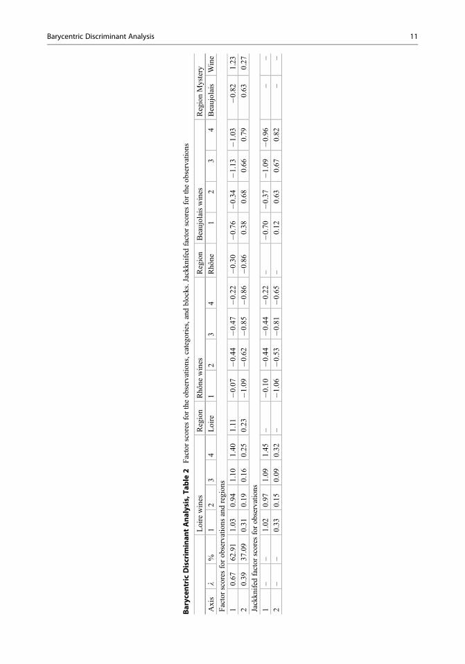
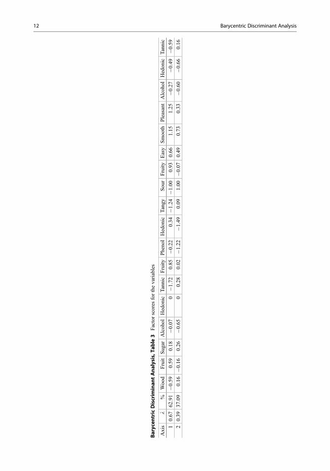
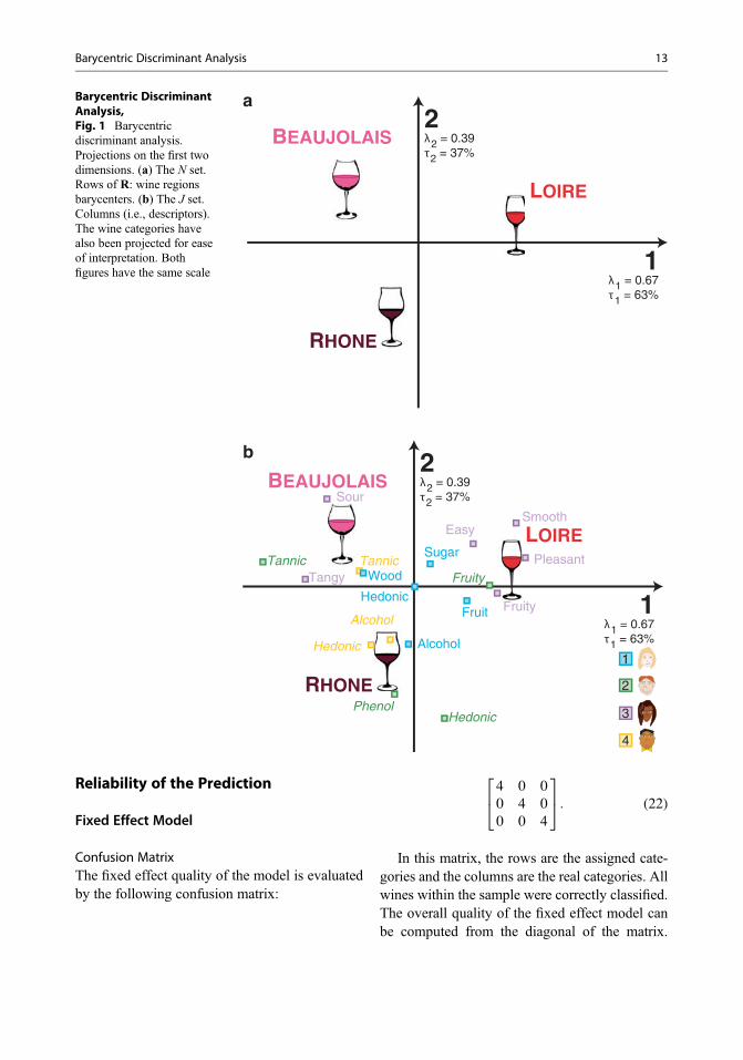
Tables 2 and 3 give the factor scores for theanalysis and Fig. 1 displays them. We can see thatthe wine regions appear to be well differentiated,with wines from the Loire being characterized as“fruity” and “pleasant,” wines from the Rhônebeing characterized as having a high “alcohol”content, and the wines from Beaujolais beingcharacterized as “tangy” and “tannic.”

Reliability and Stability of the Analysis

Proportion of Explained Variance: R2

The reliability and the stability of the analysis isevaluated by computing R2 (see Eq. 21). Its largevalue: R2 = . 94 confirms that the wine regionsare well identified. In addition, the p-value ofp < .001 (obtained from a permutation testusing 10,000 permutations) indicates that the dis-crimination of the three wine regions is reliable.

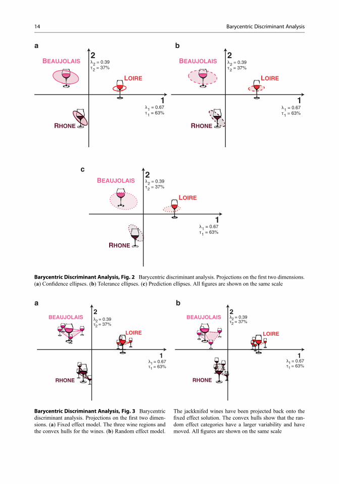
Confidence IntervalsThe original I ' J matrix was resampled 1000times with replacement, and the barycenters foreach wine region for each of the 1000 sampleswere projected onto the original factor space. The950 closest barycenters were kept, and we gener-ated the 95% confidence ellipsoid which com-prised these 950 barycenters. These confidenceellipsoids are displayed in Fig. 2a. Because thereis no overlap between the three wines regions,they are significantly different at the p < . 05significance level.


BarycentricDiscrim

inan

tAna

lysis,Ta

ble1

Datafrom

thethreewineregion

sexam

ple:12

wines

from

threedifferentw

ineregion

sareratedon

a7-po

intscaleon

descriptors

assign

edby

each

offour

assessors

Assessor1

Assessor2

Assessor3

Assessor4

Wine

Région

Woo

dFruit

Sugar

Alcoh

olHedon

icTann

icFruity

Phenol

Hedon

icTang

ySo

urFruity

Easy

Smoo

thPleasant

Alcoh

olHedon

icTann

ic1

Loire

13

21

12

52

21

13

45

41

21

2Loire

23

32

32

61

31

24

24

52

22

3Loire

12

21

22

42

42

15

35

61

13

4Loire

13

32

41

61

31

14

45

51

21

XLoire

1.25

2.75

2.50

1.50

2.50

1.75

5.25

1.50

3.00

1.25

1.25

4.00

3.25

4.75

5.00

1.25

1.75

1.75

1Rhô

ne1

21

33

33

45

31

31

13

35

12

Rhô

ne2

11

32

52

34

41

42

22

34

23

Rhô

ne3

22

21

44

46

32

21

11

23

34

Rhô

ne2

33

34

56

55

31

11

23

33

4

XRhô

ne2.00

2.00

1.75

2.75

2.50

4.25

3.75

4.00

5.00

3.25

1.25

2.50

1.25

1.50

2.25

2.75

3.75

2.50

1Beaujolais

31

31

15

41

14

41

22

23

51

2Beaujolais

21

31

26

42

14

33

33

41

24

3Beaujolais

32

22

47

41

25

51

22

11

14

4Beaujolais

31

11

36

11

14

52

13

21

24

XBeaujolais

2.75

1.25

2.25

1.25

2.50

6.00

3.25

1.25

1.25

4.25

4.25

1.75

2.00

2.50

2.25

1.50

2.50

3.25

Mystery

13

22

12

61

31

14

45

51

22


BarycentricDiscrim

inan

tAna

lysis,Ta

ble2

Factor

scores

fortheob

servations,categories,andblocks.Jackk

nifedfactor

scores

fortheob

servations

Loire

wines

Region

Rhô

newines

Region

Beaujolaiswines

RegionMystery

Axis

l%

12

34

Loire

12

34

Rhô

ne1

23

4Beaujolais

Wine

Factor

scores

forob

servations

andregion

s1

0.67

62.91

1.03

0.94

1.10

1.40

1.11

#0.07

#0.44

#0.47

#0.22

#0.30

#0.76

#0.34

#1.13

#1.03

#0.82

1.23

20.39

37.09

0.31

0.19

0.16

0.25

0.23

#1.09

#0.62

#0.85

#0.86

#0.86

0.38

0.68

0.66

0.79

0.63

0.27

Jackkn

ifed

factor

scores

forob

servations

1–

–1.02

0.97

1.09

1.45

–#0.10

#0.44

#0.44

#0.22

–#0.70

#0.37

#1.09

#0.96

––

2–

–0.33

0.15

0.09

0.32

–#1.06

#0.53

#0.81

#0.65

–0.12

0.63

0.67

0.82

––


BarycentricDiscrim

inan

tAna

lysis,Ta

ble3

Factor

scores

forthevariables

Axis

l%

Woo

dFruit

Sugar

Alcoh

olHedon

icTann

icFruity

Phenol

Hedon

icTang

ySo

urFruity

Easy

Smoo

thPleasant

Alcoh

olHedon

icTann

ic

10.67

62.91

#0.59

0.59

0.18

#0.07

0#1.72

0.85

#0.22

0.34

#1.24

#1.00

0.93

0.66

1.15

1.25

#0.27

#0.49

#0.59

20.39

37.09

0.16

#0.16

0.26

#0.65

00.28

0.02

#1.22

#1.49

0.09

1.00

#0.07

0.49

0.73

0.33

#0.60

#0.66

0.16


Reliability of the Prediction

Fixed Effect Model

Confusion MatrixThe fixed effect quality of the model is evaluatedby the following confusion matrix:

4 0 00 4 00 0 4

2

4

3

5: (22)

In this matrix, the rows are the assigned cate-gories and the columns are the real categories. Allwines within the sample were correctly classified.The overall quality of the fixed effect model canbe computed from the diagonal of the matrix.

1λ1 = 0.67τ1 = 63%

2λ2 = 0.39τ2 = 37%

LOIRE

RHONE

BEAUJOLAIS

1λ1 = 0.67τ1 = 63%

2λ2 = 0.39τ2 = 37%

3

1

2

4

Tannic

Hedonic

Alcohol

Tangy

Sour

Fruity

Easy Smooth

Pleasant Tannic Fruity

Phenol Hedonic

Wood

Fruit

Sugar

Alcohol

Hedonic

LOIRE

RHONE

BEAUJOLAIS

a

b

Barycentric DiscriminantAnalysis,Fig. 1 Barycentricdiscriminant analysis.Projections on the first twodimensions. (a) The N set.Rows of R: wine regionsbarycenters. (b) The J set.Columns (i.e., descriptors).The wine categories havealso been projected for easeof interpretation. Bothfigures have the same scale


1λ1 = 0.67τ1 = 63%

2λ2 = 0.39τ2 = 37%

LOIRE

RHONE

BEAUJOLAIS

1λ1 = 0.67τ1 = 63%

2λ2 = 0.39τ2 = 37%

LOIRE

RHONE

BEAUJOLAIS

1λ1 = 0.67τ1 = 63%

2λ2 = 0.39τ2 = 37%

LOIRE

RHONE

BEAUJOLAIS

a b

c

Barycentric Discriminant Analysis, Fig. 2 Barycentric discriminant analysis. Projections on the first two dimensions.(a) Confidence ellipses. (b) Tolerance ellipses. (c) Prediction ellipses. All figures are shown on the same scale

1λ1 = 0.67τ1 = 63%

2λ2 = 0.39τ2 = 37%

LOIRE

RHONE

BEAUJOLAIS

1λ1 = 0.67τ1 = 63%

2λ2 = 0.39τ2 = 37%

LOIRE

RHONE

BEAUJOLAIS

a b

Barycentric Discriminant Analysis, Fig. 3 Barycentricdiscriminant analysis. Projections on the first two dimen-sions. (a) Fixed effect model. The three wine regions andthe convex hulls for the wines. (b) Random effect model.

The jackknifed wines have been projected back onto thefixed effect solution. The convex hulls show that the ran-dom effect categories have a larger variability and havemoved. All figures are shown on the same scale


Here we find that all 12 wines were correctlyclassified.

The projections of the wines within the sampleinto the original GPCA space are shown inFig. 3a. The quality of the model can be evaluatedby drawing the convex hull of each category. Forthe fixed effect model, the center of gravity of theconvex hulls are the category barycenters.

Tolerance IntervalsThe reliability of the prediction for the fixed effectmodel can also be displayed graphically as toler-ance ellipsoids. These are shown in Fig. 2b. Over-lap, between the tolerance ellipsoids, representsthe proportion of misclassification of observationswithin the sample. Because there is no overlap,there were no misclassified wines within thesample.

Random Effect Model

Confusion MatrixA jackknife procedure was used in order to eval-uate the generalization capacity of the analysis tonew wines. Each wine was taken out of the sam-ple, in turn, a GPCA was performed on theremaining sample of 11 wines, and the left-outwine was then projected onto the discriminantfactor space (see Eq. 14) and was assigned to itsclosest category. This gave the following randomeffect confusion matrix:

4 0 00 4 00 0 4

2

4

3

5: (23)

The random effect performance is perfect, withall 12 wines correctly assigned.

Prediction IntervalsThe projections of the jackknifed wines onto theoriginal GPCA space (computed according toEqs. 15 and 16) are given in Table 2 and displayedin Fig. 3b. The quality of the model can be illus-trated by drawing the convex hull for these

observations. All the wines were correctly classi-fied, but note that, compared to the fixed effect (cf. Fig. 3a), the placement of the convex hull expands and shifts for each of the three wine categories.

The reliability of the predictions for the ran-dom effect model can also be displayed as predic-tion ellipsoids. Overlap between ellipsoids represents the proportion of misclassifications of new observations. This is shown in Fig. 2c. Because there is no overlap between the predic-tion ellipsoids, the new observations were all cor-rectly classified.

Extensions of BADA

Discriminant Correspondence Analysis When the observations are described by qualitative variables, the standard version of BADA cannot be used because, BADA – being based on the principal component analysis of the barycentric matrix – requires quantitative variables. Corre-spondence analysis and multiple correspondence analysis – extensions of principal component analysis for qualitative data – can, in this case, be substituted to PCA. BADA then becomes Dis-criminant Correspondence Analysis (DICA, see Abdi et al. 2012a, b; Abdi 2007b; Ben-zécri 1977; Nakache et al. 1977; Williams et al. 2010) –also known as Correspondence Dis-criminant Analysis (see Doledec and Ches-sel 1994; Perriere et al. 1996).

Multiblock Analysis (MUBADA, MUSUBADA)

Because BADA is based on GPCA, it can also analyze data tables obtained by the concatenation of data-tables or data matrices that we call here blocks (aka subtables). In this case, BADA becomes multitable (or multiblock) barycentric discriminant analysis (MUBADA Abdi et al. 2012a) and when the blocks are subjects (e.g.,


here, the assessors): multisubject barycentric dis-criminant analysis (MUSUBADA (Abdi et al.2012b)).

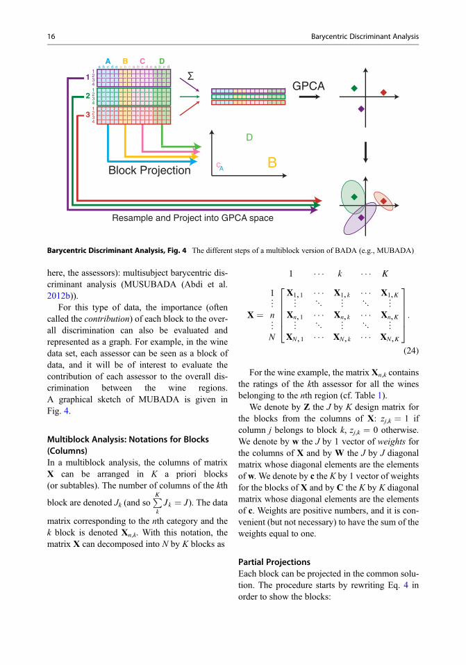
For this type of data, the importance (oftencalled the contribution) of each block to the over-all discrimination can also be evaluated andrepresented as a graph. For example, in the winedata set, each assessor can be seen as a block ofdata, and it will be of interest to evaluate thecontribution of each assessor to the overall dis-crimination between the wine regions.A graphical sketch of MUBADA is given inFig. 4.

Multiblock Analysis: Notations for Blocks(Columns)In a multiblock analysis, the columns of matrixX can be arranged in K a priori blocks(or subtables). The number of columns of the kth

block are denoted Jk (and soPK

kJk ¼ J). The data

matrix corresponding to the nth category and thek block is denoted Xn,k. With this notation, thematrix X can decomposed into N by K blocks as

1 ( ( ( k ( ( ( K

X ¼

1⋮n⋮N

X1, 1 ( ( ( X1, k ( ( ( X1,K⋮ ⋱ ⋮ ⋱ ⋮Xn, 1 ( ( ( Xn, k ( ( ( Xn,K⋮ ⋱ ⋮ ⋱ ⋮XN, 1 ( ( ( XN, k ( ( ( XN,K

2

66664

3

77775:

(24)

For the wine example, the matrix Xn,k containsthe ratings of the kth assessor for all the winesbelonging to the nth region (cf. Table 1).

We denote by Z the J by K design matrix forthe blocks from the columns of X: zj,k = 1 ifcolumn j belongs to block k, zj,k = 0 otherwise.We denote by w the J by 1 vector of weights forthe columns of X and by W the J by J diagonalmatrix whose diagonal elements are the elementsof w. We denote by c the K by 1 vector of weightsfor the blocks of X and by C the K by K diagonalmatrix whose diagonal elements are the elementsof c. Weights are positive numbers, and it is con-venient (but not necessary) to have the sum of theweights equal to one.

Partial ProjectionsEach block can be projected in the common solu-tion. The procedure starts by rewriting Eq. 4 inorder to show the blocks:

B

ΣGPCA

Block Projection

Resample and Project into GPCA space

c db ea a b c a b c d e a b c dA B C D

1234

1234

1234

1

2

3

AC

D

Barycentric Discriminant Analysis, Fig. 4 The different steps of a multiblock version of BADA (e.g., MUBADA)


R ¼ PDQ⊺ ¼ PD Q1, . . . , Qk, . . . , QK½ *⊺, (25)

where Qk is the kth block (comprising the Jkcolumns of Q corresponding to the Jk columnsof the kth block). Then, Eq. 5 is rewritten to get theprojection for the k-th block as

Fk ¼ KXkWkQk (26)

(whereWk is the weight matrix for the Jk columnsof the k-th block).

Inertia of a Block

Recall from Eq. 6 that, for a given dimension, thevariance of the factor scores of all the J columns ofmatrix R is equal to the eigenvalue of this dimen-sion. Because each block comprises a set of col-umns, the contribution of a block to a dimensioncan be expressed as the sum of this dimensionsquared factor scores of the columns of thisblock. Precisely, the inertia for the kth table andthe ‘th dimension is computed as:

Barycentric DiscriminantAnalysis, Table 4 Partialfactor scores for the blocks(i.e., assessors)

RegionsAxis Assessor Loire Rhône Beaujolais

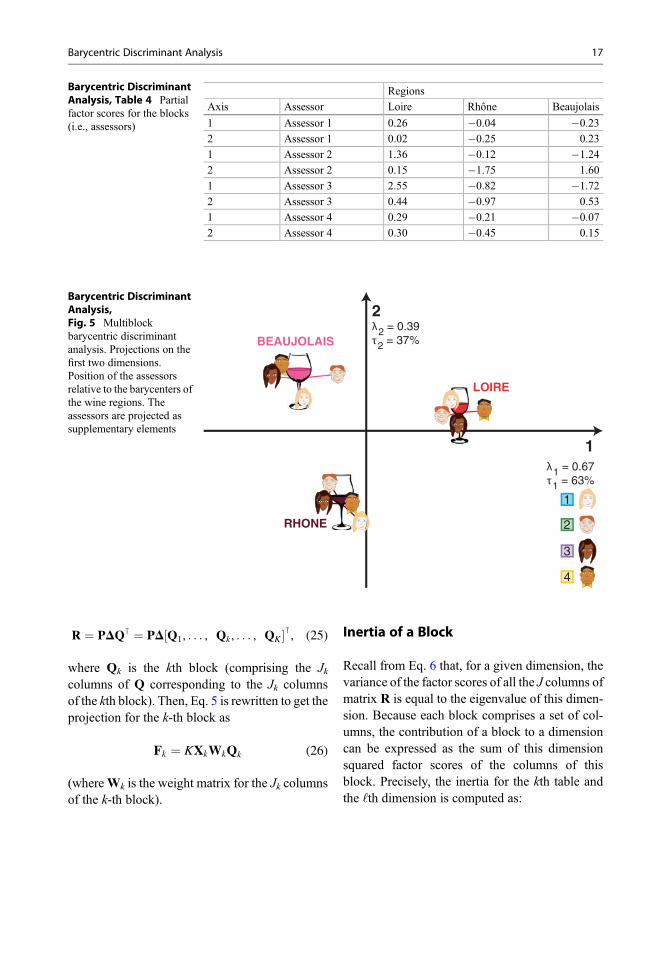
1 Assessor 1 0.26 #0.04 #0.232 Assessor 1 0.02 #0.25 0.231 Assessor 2 1.36 #0.12 #1.242 Assessor 2 0.15 #1.75 1.601 Assessor 3 2.55 #0.82 #1.722 Assessor 3 0.44 #0.97 0.531 Assessor 4 0.29 #0.21 #0.072 Assessor 4 0.30 #0.45 0.15

1λ1 = 0.67τ1 = 63%

2λ2 = 0.39τ2 = 37%

3

1

2

4

LOIRE

RHONE

BEAUJOLAIS

Barycentric DiscriminantAnalysis,Fig. 5 Multiblockbarycentric discriminantanalysis. Projections on thefirst two dimensions.Position of the assessorsrelative to the barycenters ofthe wine regions. Theassessors are projected assupplementary elements


I ‘, k ¼X

j� Jk

wj f2‘, j: (27)

Note that the sum of the inertia of the blocksgives back the total inertia:

l‘ ¼X

k

I ‘, k: (28)

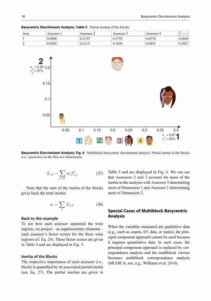
Back to the exampleTo see how each assessor separated the wineregions, we project – as supplementary elements –each assessor’s factor scores for the three wineregions (cf. Eq. 26). These factor scores are givenin Table 4 and are displayed in Fig. 5.

Inertia of the BlocksThe respective importance of each assessor (i.e.,block) is quantified by its associated partial inertia(see Eq. 27). The partial inertias are given in

Table 5 and are displayed in Fig. 6. We can seethat Assessors 2 and 3 account for most of theinertia in the analysis with Assessor 3 determiningmost of Dimension 1 and Assessor 2 determiningmost of Dimension 2.

Special Cases of Multiblock BarycentricAnalysis

When the variables measured are qualitative data(e.g., such as counts, 0/1 data, or ranks), the prin-cipal component approach cannot be used becauseit requires quantitative data. In such cases, theprincipal component approach is replaced by cor-respondence analysis and the multiblock versionbecomes multiblock correspondence analysis(MUDICA, see, e.g., Williams et al. 2010).

Barycentric Discriminant Analysis, Table 5 Partial inertias of the blocks

Axis Assessor 1 Assessor 2 Assessor 3 Assessor 4 � = l1 0.0408 0.2139 0.3743 0.0370 0.66602 0.0302 0.2113 0.1056 0.0456 0.3927

0.05 0.1 0.15 0.2 0.25 0.3 0.35 0.4

0.05

0.1

0.15

0.2

1

2λ

2 = 0.39

τ2 = 37%

λ1 = 0.67

τ1 = 63%31 2 4

Barycentric Discriminant Analysis, Fig. 6 Multiblock barycentric discriminant analysis. Partial inertia of the blocks(i.e., assessors) on the first two dimensions


Related Methods

In the same way that linear discriminant analysiscan be considered as a particular case of canonicalcorrelation analysis when one of the matrices is a“design matrix” (i.e., a matrix that codes the groupto which each observation belongs, also called a“group matrix”), BADA can be considered as aparticular case of Tucker’s interbattery analysis((Tucker 1958) also known as co-inertia analysis(Chessel and Mercier 1993; Doledec and Chessel1994), partial-least square correlation, PLSC(Krishnan et al. 2010)) when one of the matricesused is a design matrix. In the framework ofPLSC, BADA is equivalent to “mean-centered-PLSC” (Krishnan et al. 2010). Along similarlines, BADA is also a particular case ofconstrained principal component analysis(Takane 2013) when one of the data matricesused by the method is a group matrix.

The multiblock or multisubject versions ofBADA (i.e., MUBDADA and MUSUBADA)are also closely related to other multitables tech-niques such as multiple factor analysis (Abdi et al.2013) and the STATIS family of techniques (Abdiet al. 2012c).

Implementation

BADA and several related methods such asMUBADA, MUSUBADA, DICA, and MUDICAare available from several R packages including,among others, TExPosition (Beaton et al. 2014)and ade4 (but often under different names (Drayand Dufour 2007)).

Key Applications

BADA and its derivatives – or variations thereof –are used when the analytic problem is to assignobservation to predefined categories, and thismakes these techniques ubiquitous in almost anydomains of inquiry from marketing to brain imag-ing genetics (and other “omics”) and networkanalysis.

Future Directions

BADA is still a domain of intense research withfuture developments likely to be concerned withmultitable extensions (e.g., (Horst 1961)),“robustification,” and sparsification (Witten et al.2009). All these approaches will make BADA andits related techniques even more suitable for theanalysis of very large data sets that are becomingprevalent in analytics.

Cross-References

▶Canonical Correlation Analysis, Correspon-dence Analysis

▶Eigenvalues, Singular Value Decomposition▶ Iterative Methods for Eigenvalues/Eigenvectors

▶Least Squares▶Matrix Algebra, Basics of▶Matrix Decomposition▶ Principal Component Analysis▶Regression Analysis▶ Spectral Analysis▶Visualization of Large Networks

References

Abdi H (2003) Multivariate analysis. In: Lewis-Beck M,Bryman A, Futing T (eds) Encyclopedia for researchmethods for the social sciences. Sage, Thousand Oaks,pp 699–702

Abdi H (2007a) Singular value decomposition (SVD) andgeneralized singular value decomposition (GSVD). In:Salkind NJ (ed) Encyclopedia of measurement andstatistics. Sage, Thousand Oaks, pp 907–912

Abdi H (2007b) Discriminant correspondence analysis(DICA). In: Salkind NJ (ed) Encyclopedia of measure-ment and statistics. Sage, Thousand Oaks, pp 270–275

Abdi H, Williams LJ (2010a) Jackknife. In: Salkind NJ(ed) Encyclopedia of research design. Sage, ThousandOaks

Abdi H, Williams LJ (2010b) Principal component analy-sis. Wiley Interdiscip Rev: Comput Stat 2:433–459

Abdi H, Williams LJ (2010c) Barycentric discriminantanalysis (BADIA). In: Salkind NJ (ed) Encyclopediaof measurement and statistics. Sage, Thousand Oaks,pp 64–65

Abdi H, Dunlop JP, Williams LJ (2009) How to computereliability estimates and display confidence and


tolerance intervals for pattern classifiers using the boot-strap and 3-way multidimensional scaling (DISTATIS).NeuroImage 45:89–95

Abdi H,Williams LJ, Beaton D, Posamentier M, Harris TS,Krishnan A, Devous MD (2012a) Analysis of regionalcerebral blood flow data to discriminate amongAlzheimer’s disease, fronto-temporal dementia, andelderly controls: a multi-block barycentric discriminantanalysis (MUBADA) methodology. J Alzheimer Dis31:s189–s201

Abdi H, Williams LJ, Connolly AC, Gobbini MI, DunlopJP, Haxby JV (2012b) Multiple subject Barycentricdiscriminant analysis (MUSUBADA): how to assignscans to categories without using spatial normalization.Comput Math Methods Med 2012:1–15. https://doi.org/10.1155/2012/634165

Abdi H, Williams LJ, Valentin D, Bennani-DosseM (2012c) STATIS and DISTATIS: optimum multi-table principal component analysis and three way met-ric multidimensional scaling. Wiley Interdiscip Rev:Comput Stat 4:124–167

Abdi H, Williams LJ, Valentin D (2013) Multiple factoranalysis: principal component analysis for multi-tableand multi-block data sets. Wiley Interdiscip Rev:Comput Stat 5:149–179

Bastin C, Benzécri JP, Bourgarit C, Caze P (1982) Pratiquede l’Analyse des Données. Dunod, Paris, pp 102–104

Beaton D, Chin Fatt CR, Abdi H (2014) An ExPosition ofmultivariate analysis with the singular value decompo-sition in R. Comput Stat & Data Anal 72:176–189

Benzécri J-P (1977) Analyse discriminante et analysefactorielle. Les Cahiers de l’Analyse des Données2:369–406

Bergougnan D, Couraud C (1982) Pratique de la discrim-ination barycentrique. Les Cahiers de l’Analyse desDonnées 7:341–354

Celeux P, Nakache JP (1994) Analyse discriminante survariables qualitatives. Polytechnica, Paris

Chessel D, Mercier P (1993) Couplage de tripletstatistiques et liaisons espèce-environnement. In:Lebreton JD, Asselain B (eds) Biométrie etEnvironnement. Dunod, Paris, pp 15–43

Cioli C, Abdi H, Beaton D, Burnod Y, Mesmoudi S (2014)Human cortical gene expression and properties of func-tional networks. PLoS One 9(12):1–28

Diaconis P, Efron B (1983) Computer-intensive methods instatistics. Scientific American 248:116–130

Doledec S, Chessel D (1994) Co-inertia analysis: an alter-native method for studying species- environment rela-tionships. Freshw Biol 31:277–294

Dray S, Dufour AB (2007) The ade4 package:implementing the duality diagram for ecologists.J Stat Softw 22(4):1–20

Efron B, Tibshirani RJ (1993) An introduction to the boot-strap. Chapman & Hall, New York

El Behi M, Sanson C, Bachelin C, Guillot-Noel L,Fransson J, Stankoff B, Maillart E, Sarrazin N,Guillemot V, Abdi H, Rebeix I, Fontaine B, Zujovic V(2017) Adaptive human immunity drives remyelinationin a mouse model of demyelination. Brain140(4):967–980

Gittins R (1980) Canonical analysis: a review with appli-cations in ecology. Springer Verlag, New York

Greenacre MJ (1984) Theory and applications of corre-spondence analysis. Academic Press, London

Horst P (1961) Relations among m sets of measures.Psychometrika 26:129–149

Krishnan A, Williams LJ, McIntosh AR, Abdi H (2010)Partial least squares (PLS) methods for neuroimaging: atutorial and review. NeuroImage 56:455–475

Krzanowski WJ, Radley D (1989) Nonparametric confi-dence and tolerance regions in canonical variate analy-sis. Biometrics 45:1163–1173

Leclerc A (1976) Une etude de la relation entre une vari-able qualitative et un groupe de variables qualitatives.Int Stat Rev 44:241–248

Manly BFJ (1997) Randomization, bootstrap, and MonteCarlo methods in biology, 2nd edn. Chapman & Hall,New York

Nakache J-P, Lorente P, Benzcri J-P, Chastang J-F(1977) Aspects pronostiques et therapeutiques del’infarctus myocardique aigu compliqu d’unedfaillance sévère de la pompe cardiaque. Applicationdes methodes de discrimination Les Cahiers del’Analyse des Données 2:415–434

Perriere G, Lobry JR, Thioulouse J (1996) Correspondencediscriminant analysis: a multivariate method for com-paring classes of protein and nucleic acid sequences.CABIOS 12:519–524

Saporta G, Niang N (2006) Correspondence analysis andclassification. In: Greenacre M, Blasius J (eds) Multiplecorrespondence analysis and related methods. BocaRaton, Chapman & Hall/CRC, pp 371–392

St. Laurent M, Abdi H, Burianová H, Grady GL(2011) Influence of aging on the neural correlates ofautobiographical, episodic, and semantic memoryretrieval. J Cogn Neurosci 23:4150–4163

Takane Y (2013) Constrained principal component analy-sis and related techniques. CRC Press, Boca Raton

Tucker LR (1958) An inter-battery method of factor anal-ysis. Psychometrika 23:111–136

Williams LJ, Abdi H, French R, Orange JB(2010) A tutorial on multi-block discriminant corre-spondence analysis (MUDICA): a new method foranalyzing discourse data from clinical populations.J Speech Lang Hear Res 53:1372–1393

Witten DM, Tibshirani R, Hastie T (2009) A penalizedmatrix decomposition, with applications to sparse prin-cipal components and canonical correlation analysis.Biostatistics 10:515–534


https://doi.org/10.1155/2012/634165

https://doi.org/10.1155/2012/634165

barycentric discriminant analysis

Documents