Bankruptcy and Investment:

Evidence from Changes in Marital Property Laws in the U.S.

South, 1840-1850∗

Peter Koudijs† Laura Salisbury‡

March 20, 2017

Abstract

We study the impact of marital property legislation passed in the U.S. South in the 1840s onhousehold investment. These laws protected the assets of newly married women from creditorsin a world with limited debtor protection. We compare couples married after the passage ofa law with couples from the same state who were married before. Consistent with a simpleinvestment model that trades off agency costs against risk sharing, we find that the effect onhousehold investment was heterogeneous: if most household assets came from the husband(wife), the law led to an increase (decrease) in investment.

∗We thank seminar and conference participants at UC Berkeley, Gerzensee (2015 CF meeting), NYU, Stanford, theUniversity of Minneapolis, Queen’s, the University of Zurich, and the NBER (Spring 2016 DAE and CF meetings), andin particular Effi Benmelech (discussant), Jonathan Berk, Gillian Hamilton, Eric Hilt, Ulf Lilienfeld-Toal (discussant),Hanno Lustig, Petra Moser, Joachim Voth, Lucy White, Gavin Wright, and Jeff Ziebel for comments and suggestions.All errors are our own.†Stanford University and NBER, koudijs@stanford.edu.‡York University and NBER, lsalisbu@yorku.ca.

1

1 Introduction

Personal bankruptcy is an important economic institution. In an environment with incomplete

contracts, bankruptcy protection enables risk sharing between borrowers and lenders (Zame 1993).

If entrepreneurs are more risk averse than outside financiers, the availability of bankruptcy may

stimulate investment in risky projects in need of outside finance. However, bankruptcy protection

also imposes costs by creating incentives for a borrower to shirk, engage in risk shifting, or strate-

gically default. This might impede entrepreneurs’ access to funding and reduce investment. In

other words, there is a trade-off between risk sharing and agency costs, which raises the following

questions: what is the net effect of personal bankruptcy on investment, and on what factors does

this depend?

Intuitively, the net effect of bankruptcy relief should depend on the amount of protection that is

offered. It’s a simple point, but one seldom made in the literature. We formalize this intuition in a

simple investment model, in which borrowers and lenders can only write simple debt contracts, and

these contracts are not perfectly enforceable; moral hazard on the part of borrowers generates credit

constraints, which become more severe as it becomes more difficult for lenders to recover assets.

This model predicts that the net impact of bankruptcy protection on household investment depends

critically on the share of a household’s assets that are protected. Moderate levels of relief allow for

more risk sharing, while the tightening of credit constraints is only of second order importance; this

generates an increase in investment relative to the case without protection. However, as the amount

of relief increases, the impact on credit constraints becomes first order, leading to a decrease in

investment.

It is not straightforward to demonstrate empirically that the net impact of bankruptcy protec-

tion is heterogeneous in the amount of protection offered. To do this, one would need a setting in

which otherwise similar individuals are presented with substantially different degrees of bankruptcy

protection, ideally including the case of no debtor relief. Such a setting is difficult to find. There

are large cross-country differences in the amount of debt relief, but these may reflect deeper eco-

nomic, cultural, or institutional differences. Within the U.S., there is variation in state homestead

exemption limits, which generates differences in bankruptcy protection across states (Gropp et al

[1997]). However, arguably the most important part of the bankruptcy code – the possibility to

get unsecured debts discharged – is the same for everyone.

In this paper, we study a unique historical setting in which far-reaching debtor relief was intro-

2

duced in an environment with virtually no bankruptcy protection. In our setting, the amount of

bankruptcy protection differed greatly across households, allowing us to measure the net impact of

different degrees of relief. In particular, we study the introduction of a class of married women’s

property acts in the U.S. South during the 1840s. During this period, American common law held

that married women had no economic independence from their husbands and were not allowed

to own property. These married women’s property laws minimally altered this default, protect-

ing married women’s property from seizure by the family’s creditors but otherwise preserving the

husband’s economic primacy in the household; as such, historians broadly agree that they were

intended as debt relief and nothing more (Warbasse [1987]; Chused [1983]; Kahn [1996]). These

laws were passed after the Panic of 1837 led to a spike in insolvencies in the South (McGrane [1924],

Wallis [2001]). At the time, there was very little debtor protection in the region: though households

were sometimes protected through (limited) homestead exemptions, there was no bankruptcy pro-

cedure that could lead to a discharge of debts. In response to the economic distress of the 1840s,

many state legislatures passed married women’s property acts, shielding women’s assets (usually

acquired through dowry or inheritance) from her husband’s creditors.1 These laws offered families

downside protection: if a husband became insolvent, a family could fall back on the wife’s assets

for shelter, food, school tuition fees and other necessaries. At the same time, creditors could seize

fewer assets, which may have limited access to credit. Since the laws only sheltered the assets of

the wife, the actual amount of protection differed across households depending on the wife’s share

of total family property.

These early Southern laws should not be confused with other married women’s property laws

passed in the rest of the U.S. from the mid-1840s onwards, which gave married women more

economic independence (Geddes and Lueck 2002; Doepke and Tertilt 2009). The laws passed in

the South merely shielded married women’s separate property from seizure by creditors; it did not

grant them autonomy over this property. In legal terms, the early Southern laws kept the doctrine

of coverture in place. This makes them comparable to a system of bankruptcy protection, as they

effectively removed women’s property from any interaction with the credit market: under these

laws, married women were still not allowed to write contracts, so their separate estates could not

be used to guarantee loans.

We study the impact of the Southern married women’s property acts on household investment

decisions; in particular, we look at the size and type of household investment, measured by the

1General bankruptcy rules were considered but rejected as being detrimental to creditors (Coleman [1974]).

3

possession of real estate and slaves. The married women’s property acts provide a unique source of

exogenous variation in the amount of bankruptcy protection enjoyed by households. Crucially, law

changes only applied to newlyweds: a retroactive application would have been unconstitutional, as

it would have violated the terms of existing marriage contracts (Kelly [1882]). We can therefore

compare couples in the same state, in the same census year (1850), who were married before and

after the enactment of a law; only those married after were affected. As states introduced laws at

different points in time, we can also control for the year of marriage, making sure that the time

since marriage (and age effects more generally) are not driving our results. Importantly, we can

explore heterogeneity in the effect of the laws on households. Couples with relatively affluent wives

were faced with a much higher level of protection than households in which the wife was relatively

poor. Variation in the fraction of a household’s assets owned by the wife allows us to implement

what is essentially a differences-in-differences-in-differences design. In addition, because the laws

only applied to couples married after the date of enactment (a relatively small group of people),

general equilibrium effects are not first order in the short term, allowing for a straightforward

partial equilibrium interpretation of results.

The starting point for our analysis is a simple model of household borrowing and risky in-

vestment. Following the literature on (financial) contracting, we model a household’s borrowing

decision as a moral hazard problem. We assume that if a project is successful, the household can

strategically default and divert some of the returns. To enable lending, the loan contract has to

be set up in such a way that the household never has an incentive to do this. This generates

an endogenous borrowing constraint: there has to be sufficient skin-in-the-game to warrant a cer-

tain loan size. Crucially, following the literature on bankruptcy protection (see White [2011] and

Livshits [2014] for overviews), we assume that the only financial instrument available is a simple

debt contract.2 If households are risk averse, this market incompleteness creates inefficiencies. On

the one hand, simple debt relaxes the borrowing constraint, as it minimizes the household’s debt

payments if the project is successful. On the other hand, it removes any possibility of risk sharing

(Holmstrom 1979). We show that the introduction of a married women’s property law can move the

household’s investment decision closer to what it would be if contracts were not limited to simple

debt. By protecting the wife’s assets, the household will optimally decide to increase borrowing

2This is a reasonable assumption in the context of the U.S. South in the 1840s. Kilbourne (1995; 2006) provides adetailed analysis of credit markets in the Antebellum U.S. South. There is no evidence for rich credit arrangementsthat allowed for risk sharing. Simple debt seems to have been the norm.

4

to scale up investment. This is consistent with the insights of Dubey, Geanakoplos and Shubik

(2005) and Zame (1993), who argue that bankruptcy protection can serve to make markets more

complete. We show that this will only happen if a wife’s property accounts for a relatively small

fraction of the total. If a wife’s share of total assets is high, the borrowing constraint becomes so

restrictive that investment will fall after a the enactment of a property law.

To test these predictions, we compile a new database that links records of marriages contracted

in southern states between 1840 and 1850 to the censuses of 1840 and 1850. Though we don’t observe

credit, this database does allow us to observe the gross value of real estate and slave holdings at

the household level in 1850. We can compare this measure of family assets for couples in 1850 who

were married before and after a married women’s property law. Links to the 1840 census allow

us to construct a measure of pre-marriage familial assets: average slave wealth among people with

a certain surname from a certain state. This measure captures how wealthy grooms’ and brides’

families were at the time of marriage, which approximates the quantity of assets husband and wife

brought into a union. We take 1850 gross asset holdings conditional on each partner’s pre-marital

wealth as a measure of investment.

Using our quasi differences-in-differences-in-differences approach, we find strong support for our

simple model. Married women’s property laws had a heterogeneous effect on 1850 real estate and

slave holdings: they increased investment when the bulk of a couple’s property was owned by the

husband; however, they had the inverse effect when most of a couple’s property was owned by the

wife. This result is important for two reasons. First of all, it indicates that models focusing on

borrower incentives are empirically relevant, at least in our historical data. It seems likely that

Moral Hazard on part of the borrower is a fundamental characteristic of arms’ length finance, sug-

gesting that this class of models is important for understanding the effects of bankruptcy protection

more generally. Second, our results imply that a limited amount of protection is sufficient to make

markets more complete and increase household investment. If the fraction of assets exempt in

bankruptcy is too large (we estimate that the critical level lies around 20-30%), investment falls.

This paper is directly related to the literature on the consequences of bankruptcy protection on

household borrowing and investment decisions. There is a large literature in macroeconomics that

analyzes the trade-off between risk sharing and access to credit using structural models (see for

example Athreya [2002], Livshits, MacGee and Tertilt [2007], and Chatterjee et al [2007]). In these

papers, households use credit markets primarily to smooth consumption and changes in debtor relief

5

only affect investment indirectly (Li and Sarte 2006). Closer to our paper, there is an extensive

micro-econometric literature on the topic using cross-state variation in exemptions. Conclusions

about whether higher exemptions increase or decrease credit and investment differ across studies.

Gropp et al (1997), the seminal paper in this literature, find that larger homestead exemptions

tend to redirect credit to individuals with high assets to begin with. On the other hand, Severino

et al (2013) look at a recent wave in changes in exemptions and show that higher exemptions are

associated with an increase in unsecured debt that is mainly driven by low-income households. The

reasons for these different results are not well understood. Berkowitz and White (2004), Berger,

Cerquiero and Penas (2011) and Cerquiero and Penas (2011) focus on small-business owners and

show that higher exemptions lead to less credit. Fan and White (2003) find that the probability of

starting a small business does go up. Cerqueiro et al (2014) document that higher exemptions are

related to less innovative activity, emphasizing the importance of external financing for innovation.

Relative to this literature we make the following contributions. First of all, we study a

large change in the bankruptcy regime that enables us to compare households with and with-

out bankruptcy protection. Since the new marriage laws only applied to newlyweds, we can base

our estimates on couples living in the same state who got married before and after the law change.

This means that our results do not rely on state-level variation that might reflect deeper underly-

ing economic differences (Hynes, Malani and Posner [2004]). Second, in our setting the eventual

amount of protection varies across individuals depending on the relative wealth of husband and

wife. This contrasts with the literature using (homestead) exemptions. Since the property debtors

get to keep in bankruptcy is defined in dollar terms, within-state variation in the fraction of assets

protected comes from differences in total wealth. This is likely correlated with other things, such

as access to investment projects or credit worthiness. Finally, again due to their prospective na-

ture, the new marriage laws only affected a small fraction of households, suggesting that general

equilibrium effects are not of first order importance in our setting. This enables us to interpret the

results in a straightforward partial equilibrium way. In contrast, Lilienfeld-Toal, Mookherjee, and

Visaria (2012) argue that higher exemption levels might change the credit market equilibrium in a

state, redirecting credit to the most reliable borrowers, and that this could explain Gropp et al’s

finding that richer households benefit more from higher exemptions.

The remainder of this paper is structured as follows. Section 2 provides more historical back-

ground. In Section 3, we introduce a simple model of bankruptcy protection and investment.

Section 4 describes the dataset underlying our analyses. Section 5 presents the empirical specifi-

6

cation, the main results, and a detailed exploration of alternative mechanisms that may generate

these results. Section 6 concludes.

2 Historical Background

2.1 Credit Markets

The economy of the U.S. South was centered on plantation agriculture. In the 1850 census, around

2/3 of respondents worked in agriculture, mainly cotton. According to Wright (2006), a quarter of

people owned a plantation and slavery was widespread.3 Southern families relied heavily on credit.

Commission agents frequently made short term loans to plantation owners to finance the planting

of a year’s crop. On top of that, plantation owners had access to long term loans. They either

contracted debt from outside financiers through the endorsement of local magnates, or they had

long standing “open accounts” with their commission agents.4. This long term credit allowed them

to make purchases of land, slaves and machinery (Kilbourne [1995], p. 31).

These credit arrangements were often collateralized through mortgages on the land and slaves

already in the possession of the planter. Mortgages provided endorsers with an official guarantee.

Alternatively, commission agents used the mortgages as collateral to obtain funding of their own

in national or international credit markets. As an illustration, Benjamin Kendrick, one of the

wealthiest individuals in East Feliciana Parish, Louisiana, had endorsed a number of loans for

John G. Perry in 1835. To protect Kendrick against a possible default, Perry provided him with a

mortgage on a number of slaves he had recently purchased. In another example, John McKneely

had an open account with J.W. Burbridge & Co that allowed him to run up debts with the firm

totaling $18,500. As a guarantee, McKneely pledged a mortgage on his 1000 acre estate and 50

slaves (Kilbourne [1995], p. 62, 70). Mortgages ran for a decade and could be renewed for another 10

years. Kilbourne argues that these loans were often over-collateralized. He references 16 mortgages

with detailed conditions; the average loan-to-value ratio on these loans was 45%. Table A1 has

more details. Kilbourne also documents that, at least in East Feliciana Parish, slaves were the

most important form of collateral. They constituted about 80% of the planters’ wealth. Moreover,

due to the fact that they could be easily moved and assigned different tasks, they were also much

more liquid in secondary markets than land (Wright 1986). Even though most lending centered on

3Approximately one third of white southern households report owning slaves in the 1840 federal census.4These so-called factorage firms offered a wide menu of financial services, akin to investment banks today

7

plantation agriculture, credit markets were not restricted to plantation owners. The inhabitants

of towns and cities could also mortgage their homes and town plots under similar conditions to

acquire long term loans [Kilbourne [1995], p.60].

There is no evidence for credit arrangements in the Antebellum U.S. South that allowed for risk

sharing between lenders and borrowers. Simple debt seems to have been the norm (Coleman [1974],

Kilbourne [1995, 2006], and Thomson [2004]). Upon insolvency, debtors generally had no other way

to discharge their debts than through private negotiation with their creditors. Bankruptcy relief

was virtually non-existent, and lenders could use the local court systems to press for debt repayment

through the seizure of a borrowers’ assets and by threatening to send a borrower to debtor’s prison.5

At the time, all loans were full recourse (Kilbourne [1995]; [2006]). This implied that if the specific

assets that been used to collateralize a loan were insufficient to cover repayment, the creditor could

size all other assets belonging to a borrower. If a husband’s assets were not sufficient to cover the

remaining debt, creditors could lay claim on a wife’s assets.

2.2 Introduction of the Married Women Property Laws

Prior to the introduction of married women’s property acts, married women’s property was governed

by American common law, which dictated that virtually all property owned by a woman before

marriage or acquired after marriage belonged to her husband. 6 In most of the states we consider

in our empirical analysis, prenuptial agreements were problematic to enforce and therefore rare

(Salmon 1986, p. xv). The key difficulty lay in the dual legal system in the U.S. at the time. The

dominant legal framework was American common law. Under this system, prenuptial agreements

were not valid. To ‘fix’ some of the inequities of common law, a separate body of equity law had

evolved. This branch of the law did support prenuptial agreements, but it was less well established

and was administered in separate chancery courts. This created two problems. First, as many

southern states did not structurally report equity cases, judges often knew little of the equity

jurisprudence. Second, there were few courts that solely administered equity law. Usually, a judge

mixed equity and common law cases. As a result, decisions were rife with inconsistencies (Warbasse

5Debtor’s prison was only abolished after the Civil War (Coleman [1974], p. 243). In the 1840s and 1850s it wasa tool that was predominantly used to force borrowers to give up their remaining assets. Most states put restrictionson the use of debtor’s prison. Generally, a borrower could get a quick release from prison after assignment of hisproperty to his creditors. If lenders refused to free borrowers, they had to assume the costs of imprisonment.

6The exception was real estate. Although the fruits derived from real estate belonged to the husband (who coulduse this revenue as collateral for a loan), the property itself was inalienable and was held in trust by the husband forhis wife. It was supposed to pass on to their children or otherwise would revert back to the wife’s family (Warbasse1987, p.9).

8

1987, p. 165-6). A series of legal cases from Alabama demonstrate how difficult is was to protect a

wife’s property by ways of an prenuptial agreement. In O’Neil v. Teague (8 Ala. 345) a father had

bequeathed two slaves to his daughter’s trustees as her separate property right after her wedding

in 1843. Nevertheless, in 1844 the court decided that the slaves could be seized to satisfy the debts

contracted by the daughter’s husband in 1839.7. In Michan v. Wyatt (21 Ala 813), the husbands’

creditors had seized slaves from a wife’s separate estate in 1843. The family had to prosecute for

nine years to get them back.

Warbasse (1987) suggests that the problems associated with equity law and prenuptial agree-

ments spurred the passing of state statutes modifying the common law to better protect women’s

assets within a marriage. These laws were introduced at different times in different states.8 The acts

can be broadly separated into four categories: debt relief, or acts that shielded women’s property

from seizure by husbands’ creditors but did not allow women to control their separate property;

property laws, or laws that allowed women to independently own and dispose of real and personal

property; earnings laws, which allowed women to control their own labour earnings; and sole trader

laws, which allowed women to engage in contracts and business without their husbands’ consent.

We focus on the first class of married women’s property acts (“debt relief”), which were enacted

in most southern states during the 1840s. The states that did not pass these laws had the most well

developed equity law systems, such as Virginia (Warbasse 1987, p. 167). The passing of these laws

followed a major recession after the Panic of 1837, which was caused by a large decline in cotton

prices (Temin [1969]). This depressed land and slave prices in the southern states, where the

economy and financial system was largely based around plantation agriculture (McGrane [1924]).

After a brief recovery, the U.S. economy entered a phase of strong deflation in 1839, which made

it hard for debtors to repay their loans (Wallis [2001]). In response to the crisis, the national

government implemented a controversial federal bankruptcy law in the summer of 1841 that allowed

thousands of families to file for voluntary bankruptcy and qualify for debt forgiveness. The law was

very unpopular with creditors and was repealed within a year (Coleman [1974], p. 23). It would

take until 1898 before a permanent federal bankruptcy code was finally introduced.9

The absence of a federal bankruptcy law led a number of states to introduce (limited) forms

of debtor protection at the state level. The introduction of the married women’s property laws

7For similar cases see 2 Port 463, 8 Port 73, 2 Ala 152, 12 Ala 42, 15 Ala 169, and 16 Ala 181.8Information on married women’s property acts is compiled from a number of sources, including Kahn (1996),

Geddes and Lueck (2002), Warbasse (1987), Kelly (1882), Wells (1878), Chused (1983) and Salmon (1982).9All our results are robust to the exclusion of couples who got married before the summer of 1842.

9

was an important element of these policies. According to Warbasse (1987, p. 180) the Southern

legislatures responded to “the financial debacle which followed the Panic of 1837, [when] widespread

land foreclosures brought to public attention the incredible hardships imposed upon wives whose

estates were taken to pay for husbands’ debts”. For example, an article in the 1843 Tennessee

Observer states that “the reverses of the last few years have shown so much devastation of married

women’s property by the misfortunes of their husbands, that some new modification of the law

seems the dictate of justice as well as prudence”. The Georgia Journal argued in the same year

that there is no good reason “why property bequeathed to a daughter should go to pay debts of

which she knew nothing, had no agency in creating, and the payment of which, with her means,

would reduce her and her children to beggary. This has been done in hundreds of instances, and

should no longer be tolerated by the laws of the land” (quoted in Warbasse [1987], p. 176-177).

Furthermore, Warbasse argues that a change in marriage laws “appealed to the self-interest of

indebted landholders who might henceforth retain control of their wives’ property without fearing

its confiscation by creditors”.10 This seems to have been a widespread sentiment, and even states

that did not succeed in passing a married women’s property act during the 1840s proposed them

to the state legislature. For example, Georgia failed to pass an act in 1843 by a margin of 18 out

of 173 votes. Around the same time, states also introduced bankruptcy exemptions under which

lenders could not seize borrower’s property up to a specific maximum value, usually around $500

($16,000 in today’s money) (Farnam [1938]).11

Table 1 contains a list of important legislative dates for each state that we use in our analysis.

The first married women’s property law was passed in Mississippi in 1839, which merely sheltered a

woman’s slaves from seizure by her husband’s creditors; an additional law was passed there in 1846,

securing the income earned from her real and personal property to her separate estate. Alabama,

Florida, Kentucky, North Carolina, and Tennessee all passed similar property laws during the

1840s. Virginia and Georgia did not pass laws during the period, and Louisiana and Texas were

community property states which kept property owned before marriage separate prior to the 1840s.

Arkansas passed a weak version of a property law in 1846, which was generally considered nothing

more than a strengthening of the equity tradition, which governs premarital contracts (Warbasse

[1987]). In all cases, the statutes did not grant women the right to control their separate property;

it was kept in a trust administered by their husbands. As Kahn (1996) writes, “control remained

10Goodman (1993, p.488-9), Kahn (1996, p. 361) and Thompson (2004, p. 26, 91-2) make a similar argument.11In one of our robustness tests in Section IV we show that the introduction of exemptions cannot explain our

findings.

10

with the husband, and courts interpreted the legislation narrowly to ensure that ownership did not

signify independence from the family” (p. 361).

2.3 The Impact of the Married Women Property Laws

The married women’s property acts passed in the South during the 1840s did not grant women

economic independence, but they did place real constraints on the way in which their property

was used. As said, wives’ assets were protected from husbands’ creditors. For example, in Frost v.

Doyle (15 Miss 68) a husband had used his wife’s estate to secure a number of promissory notes.

When the creditor tried to seize the collateral, the court ruled against this, stating that “the notes

did not constitute a valid charge”. At the same time, a wife could not contract debt in her own

name. Under common law a married women (or ‘feme covert’) did not have the power to contract;

common law assumed that a family was a single legal entity, led by the husband (Kelly [1882], p.

22). The early married women’s property acts did not (yet) change this. For example, a Mississippi

decision from 1846 held that “[the law] has not the effect to extend [a wife’s] power of contracting,

or of binding herself or her property; its effect rather is to take away all power of subjecting her

property to her contracts” (15 Miss 64). This put a wife’s assets in a special position: neither

husband nor wife could use them as collateral to obtain credit.

In general, husbands and wives were allowed to jointly sell wife’s assets. However, this did not

mean that the ownership changed or that proceeds could be consumed. The proceeds from the

sale had to be reinvested as part of the wife’s separate estate. For example, an Alabama decision

from 1857 maintains that, even if a wife’s property can be sold by a husband and wife jointly, the

proceeds “are to be reinvested in ‘the purchase of other property’ – not sold for money” (31 Ala.

39). The statute was interpreted to protect a wife’s property “not only against third persons, but

against the husband himself.” This principle seems to have been broadly upheld in court.

At the same time, the law did make exceptions to prevent hardship on part of the family. For

example, a wife’s property could generally be used for “common law necessaries” which included

food, shelter, and sometimes school fees, if the husband was unable to do so because of insolvency,

sickness or because he abandoned his family. In addition, part of the wife’s property could be sold

to pay for the maintenance of a plantation. In sum, the married women property laws had the dual

purpose of preserving the wife’s property and offering protection from adverse shocks.

Husband and wife could not simply shift assets around to optimize the ownership structure

within the marriage. Gifts from husband to wife, even if they occurred before marriage, could

11

be construed as an attempt to defraud creditors and courts often nullified such transactions. For

example, the Mississippi Acts of 1839 and 1846 explicitly stated than women could not accept

gifts from their husbands, a provision that was strictly upheld in court (for example in Ratcliffe v.

Dougherty, 24 Miss. 181). Similarly, since common law did not allow married women to make any

legally binding economic decisions, a wife was unable to transfer the ownership of her assets to her

husband. For example, the Alabama Marriage Act of 1848 stated that “husband and wife cannot

contract with each other for the sale of any property”. This was upheld in court, for example in

Reel v. Overall (39 Ala. 138).

The married women’s property acts only applied to people married after the passing of a law.

A retroactive application would have been a violation of the so-called contract clause in the Federal

Constitution stipulating that states cannot introduce laws that impair existing contracts. Alabama,

for example, explicitly stated that the Act of 1848 would not apply retroactively (Kelly [1882],

p.291). In an Alabama case in 1852 (20 Ala. 710) the court referred to 1848 Act but ignored it as

the marriage had taken place before the passing of the law.

Of course, the extent to which these laws had any meaningful impact depends on the degree to

which women held property during this period. As women’s labor force participation was very low,

women’s property would have to come from family. The historical evidence suggests that women

frequently received real estate and personal wealth from their family. The first channel was dowry.

Though there is little research on dowry in the Antebellum South, historical anecdotes suggest

that it was a frequent phenomenon. Thomas Jefferson’s wife, for example, received a dowry of 132

slaves and many thousands of acres of land (Gikandi [2011]). Auslander (2011) gives numerous

examples from Antebellum Greenwood county, Georgia of the transfer of slave property in the form

of dowry. The second channel was inheritance. After the American Revolution the United States

had done away with the British standard of primogeniture. In 1792 most US states (including

the South) had passed so-called intestacy laws that guaranteed that in the absence of a will, sons

and daughters would receive equal shares in the inheritance from their parents (Shammas et al.

[1987], p. 64-65; 83). There is very little evidence on the exact shares stipulated in actual wills,

but anecdotal evidence suggests that women could receive sizable inheritances, often in the form

of slaves (Warbasse [1987], p. 143-144; Brown [2006]).

12

3 Theory

In this section, we develop a simple model to characterize the way in which married women’s

property laws affect household borrowing and investment. The starting point is the observation

that the only financial instruments available to households at the time were simple, non-contingent,

debt contracts. In this case, offering downside protection through the exemption of the wife’s

property likely has two countervailing effects. First, it may reduce the overall amount of credit and

investment because households have less pledgeable collateral after the passage of the law. Second, it

may increase overall investment because households are risk averse: the downside protection makes

potential insolvency less disastrous and thus could encourage a family to borrow and invest more.

Effectively, bankruptcy protection helps to make markets more complete (Dubey, Geneakoplos and

Shubik [2005] and Zame [1993]). In what follows, we explore the circumstances under which each

of these two effects dominates.

Following the large theoretical literature on (financial) contracting, we model the household

investment decision as a moral hazard problem. A risk averse household can invest in a risky

project with positive net present value. If the project is successful, the household has the option to

divert some of the project’s returns. The project’s outcome is fully verifiable to the outside investor,

who can attempt to obtain legal recourse. Diverting cash flows is therefore costly, as the household

would, for example, need to abscond to a different state to evade legal action.12 To prevent this

inefficient outcome, the household needs sufficient skin-in-the-game. This endogenously generates

a collateral constraint.13

We first solve the model assuming that markets are complete, that is borrowers and lenders can

write any contract possible. This serves as a useful benchmark to better understand the efficiency

implications of the married women’s property acts. We then solve the model when only simple

debt contracts are available. A key result is that investment levels will always be lower compared

to the complete contracts case if the household is risk averse. Finally, we introduce a married

women’s property law that protects the wife’s assets from creditors. We show that if the fraction of

household assets that belongs to the wife is significant, but sufficiently small, protection will move

the household closer to the complete markets solution and investment will increase. All proofs can

12Debtors frequently moved to a different state to escape creditors’ claims (Wright [1986], p. 65). Before obtainingstatehood in 1845, Texas was a particularly popular destination since the different legal systems made it hard tocollect debts. This gave rise to the acronym G.T.T.: “Gone To Texas” (Baptist [2014], p. 287-8).

13This simple form of moral hazard greatly simplifies the analysis. The same economic intuition should hold fordifferent moral hazard problems related to effort provision (Innes [1990], Holmstrom and Tirole [1997]), semi-verifiableincome (Townsend [1979]) or non-verifiable income (Hart and Moore [1989] and Bolton and Scharfstein [1990]).

13

be found in Appendix A.

3.1 Setup

Husbands and wives enter a marriage with assets wM and wF , respectively. The household allocates

total wealth w = wM +wF between consumption today (c0) and investment, the proceeds of which

will be consumed “tomorrow” (c1). We can think of c1 as an amalgam of the couple’s future

consumption and a bequest to children. The household has log utility over current and future

consumption:

U(c0, c1) = log c0 + θE[log(c1)]

Investment takes the form of a risky project, which yields a return of R ∈ {R,R} with equal

probabilities, where R > 1 is the return if the project succeeds, and 12−1/R < R < 1 is the return

if the project fails. The lower limit on R ensures that, in an incomplete markets world without

protection, the household will always want to borrow a strictly positive amount to invest in the

risky project and does not want to store its wealth in a risk-free asset, such as government bonds.14

We define r ≡ E(R) = R+R2 > 1, so the project has a positive expected value. Further, we define

∆r ≡ R−R.

Households can obtain outside financing to scale up investment. We assume that a portion of

the project’s return can always be seized by the financier; for simplicity, we assume that this is

RI, where I is the total amount invested in the project. We can think of this as the value of the

underlying land, buildings, slaves and tools. These assets are (1) likely to retain a large fraction

of their original value, even if the project fails, and (2) are relatively easy to confiscate by the

outside investor. This means that, if the project fails, households can be forced to hand over all

their remaining assets. If the project succeeds, there will be an additional (R−R)I = ∆rI on the

table that cannot be easily seized and which the household can divert. We can think of this as

the cash proceeds of the project. Diversion is costly, and the household will only be able to keep

β∆rI, where 2(r−1)∆r < β < 1. In order for an outside financing contract to be incentive compatible,

the amount of money households are left with in the event of success must at least be as big as

β∆rI. The lower limit on β ensures that the moral hazard problem is always serious enough that

it leads to a cap on outside investment. We assume that financiers are risk neutral and competitive.

Furthermore, we normalize the risk-free rate of return to zero.

14Throughout, we make the assumption that, in case of default, risk-free assets, such as government bonds orbalances with (merchant) banks, can always be seized by creditors.

14

3.2 Complete and Incomplete Markets Without Protection

We first consider the case in which markets are complete, and the household can pick from an

unconstrained menu of contracts to obtain outside financing, e. Total investment is given by

w − c0 + e. The incentive compatibility constraint (IC) is given by

R(w − c0 + e)− ρge ≥ β∆r(w − c0 + e)

while the financier’s zero profit condition implies that

ρg + ρb = 2

where ρg (ρb) is the return to the outside investment in the good (bad) state of the world.

Proposition 1 Suppose that 2(r−1)∆r < β < 1 and 1

2−1/R < R < 1. Under complete markets, the

IC constraint is binding, and households will choose the following values of c0, e, ρg, and total

investment w − c0 + e:

c∗0 =w

1 + θ

e∗ =2r − 1− β∆r

β∆r − 2(r − 1)

θ

1 + θw

ρ∗g =R− β∆r

2r − 1− β∆r

w − c∗0 + e∗ =1

β∆r − 2(r − 1)

θ

1 + θw

It is relatively easy to see that if the household is risk neutral, the optimal contract would involve

simple risk-free debt. Since the project has positive net present value, it is optimal to loosen the

IC constraint as much as possible. This means minimizing the payment the household has to make

in the good state of the world. In the bad state of the world it pays as much as it can. Proposition

1 indicates that this changes when the household is risk averse. In that case, the optimal contract

strikes a balance between incentive compatibility and risk sharing.15 The household will have a

positive payout in the bad state of the world. To satisfy the financier’s zero profit condition, this

implies a higher payment in the good state of world.

15For other models in which incentive compatibility is traded off against risk sharing see Holmstrom (1979) andHolmstrom and Ricart-i-Costa (1986).

15

Next, we solve the model assuming that only simple debt contracts are available. In this case,

the household borrows an amount l and the lender charges a fixed interest rate ρ. Total investment

is given by w − c0 + l. If the household is able to repay the lender in the bad state of the world,

the loan is risk-free and ρ = 1. If the loan is risky, the household is forced to give up the entire

project’s return in the event of failure. The lender’s zero profit condition dictates that

ρl +R(w − c0 + l) = 2l

The IC constraint is similar to before.

Proposition 2 Under incomplete markets with no protection, the IC constraint is never binding,

and the household will choose the following values of c0, l, ρ, and total investment w − c0 + l:

c∗0 =w

1 + θ

l∗ =RR− r

(R− 1)(1−R)

θ

1 + θw

ρ∗ = 1

I∗ = w − c∗0 + l∗ =r − 1

(R− 1)(1−R)

θ

1 + θw

The household decides to contract a risk-free loan. It will never want to borrow more than

it can repay in the bad state of the world, as the lender can seize the entire return, driving the

household down to zero consumption. With a risk-free loan, the IC constraint will never bind.

Outside financing and total investment always fall relative to the complete markets case:

Lemma 3 For a given w, outside investment (e∗) and gross investment (w−c∗0+e∗) under complete

contracts are greater than borrowing (l∗) and gross investment (w − c∗0 + l∗) under incomplete

contracts with no debtor protection.

3.3 Incomplete Markets With Protection

The introduction of a married women’s property law can partly remedy the inefficiency caused by

contract incompleteness. Under the new law the proceeds from investing wF can never be seized

by the outside financier. By guaranteeing a minimum level of consumption in the bad state of the

world, the household might find it optimal to contract a large risky loan, leading to an increase

in investment. At the same time, the protection of a wife’s property can also further amplify the

16

inefficiencies through the tightening of the IC constraint. Which of these two effects dominates

depends on the relative proportions of wM and wF in total household wealth.

Under protection a household contracts a (possibly) risky loan l and total investment is given

by wM + wF − c0 + l. If the loan is indeed risky, the lender’s zero profit condition yields that

ρl +R(wM − c0 + l) = 2l

The IC is given by

R(wM − c0 + l)− ρl ≥ β∆r(w − c0 + l)

Note the absence of wF in both expressions. In line with the married women’s property laws (see

Section 2), we assume that the household can only consume wF in t = 0 after the husband’s assets

wM have been exhausted.

Proposition 4 Suppose that 2(r−1)∆r < β < 1 and 1

2−1/R < R < 1. There exist φ1 and φ2, where

φ2 > φ1, such that under incomplete contracts with wF protected, the household will choose the

following equilibrium values of c0 and l, and gross investment wM + wF − c0 + l:

Case 1. wM/wF < φ1:

c0 =1

1 + θ(wM + wF )

l = 0

I = wM + wF − c0 + l =θ

1 + θ(wM + wF )

Case 2. φ1 ≤ wM/wF < φ2:

c0 =2

2 + θ

{wM +

R(2− 2r + β∆r)

2β∆rwF

}l =

2r − β∆r

2− 2r + β∆r

θ

2 + θwM −

R(2r − β∆r)

2β∆r

2

2 + θwF

I = wM + wF − c0 + l =2

2− 2r + β∆r

θ

2 + θwM +

{1− R

β∆r

2

2 + θ

}wF

17

Case 3. wM/wF ≥ φ2:

c0 = c∗0 =wM + wF

1 + θ

l = l∗ =RR− r

(R− 1)(1−R)

θ

1 + θ(wM + wF )

I = I∗ = wM + wF − c0 + l =r − 1

(R− 1)(1−R)

θ

1 + θ(wM + wF )

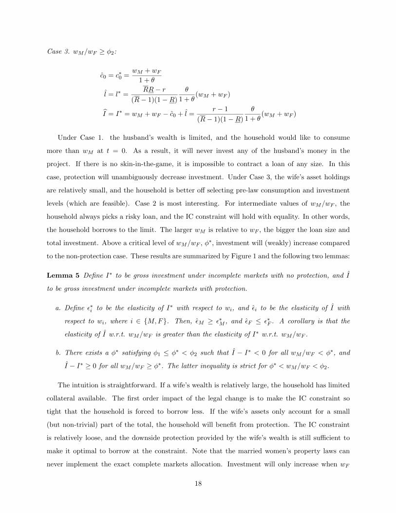
Under Case 1. the husband’s wealth is limited, and the household would like to consume

more than wM at t = 0. As a result, it will never invest any of the husband’s money in the

project. If there is no skin-in-the-game, it is impossible to contract a loan of any size. In this

case, protection will unambiguously decrease investment. Under Case 3, the wife’s asset holdings

are relatively small, and the household is better off selecting pre-law consumption and investment

levels (which are feasible). Case 2 is most interesting. For intermediate values of wM/wF , the

household always picks a risky loan, and the IC constraint will hold with equality. In other words,

the household borrows to the limit. The larger wM is relative to wF , the bigger the loan size and

total investment. Above a critical level of wM/wF , φ∗, investment will (weakly) increase compared

to the non-protection case. These results are summarized by Figure 1 and the following two lemmas:

Lemma 5 Define I∗ to be gross investment under incomplete markets with no protection, and I

to be gross investment under incomplete markets with protection.

a. Define ε∗i to be the elasticity of I∗ with respect to wi, and εi to be the elasticity of I with

respect to wi, where i ∈ {M,F}. Then, εM ≥ ε∗M , and εF ≤ ε∗F . A corollary is that the

elasticity of I w.r.t. wM/wF is greater than the elasticity of I∗ w.r.t. wM/wF .

b. There exists a φ∗ satisfying φ1 ≤ φ∗ < φ2 such that I − I∗ < 0 for all wM/wF < φ∗, and

I − I∗ ≥ 0 for all wM/wF ≥ φ∗. The latter inequality is strict for φ∗ < wM/wF < φ2.

The intuition is straightforward. If a wife’s wealth is relatively large, the household has limited

collateral available. The first order impact of the legal change is to make the IC constraint so

tight that the household is forced to borrow less. If the wife’s assets only account for a small

(but non-trivial) part of the total, the household will benefit from protection. The IC constraint

is relatively loose, and the downside protection provided by the wife’s wealth is still sufficient to

make it optimal to borrow at the constraint. Note that the married women’s property laws can

never implement the exact complete markets allocation. Investment will only increase when wF

18

is relatively small; in that case, consumption in the bad state of the world is lower than it would

be under complete contracts. Nevertheless, as long as wM/wF ≥ φ∗, post-law investment will be

(weakly) closer to investment under complete markets. In the empirical section, we will explicitly

test for Lemma 5a. and we will provide an estimate for the φ∗ defined under Lemma 5b.

4 Data

We link data from four sources: (1) county records of marriages contracted in the South between

1840 and 1850 from familysearch.org; (2) the complete count 1850 federal census from the North

Atlantic Population Project; (3) slave schedules from the 1850 federal census from ancestry.com; (4)

a complete index to the 1840 census from familysearch.org. We begin by extracting information from

approximately 250,000 marriage records from southern states dated between 1840 and 1850 from

the genealogical website familysearch.org. These electronic records contain the full name of both

the bride and the groom, the date of marriage, and the county of marriage. Once we have obtained

these marriage records, we match them to the population census and slave schedules of 1850. The

1850 data contain information on place of residence, birth place, birth year, household composition,

occupation, literacy, the value of real estate assets and slave holdings. Real estate assets included

all land and buildings a household owned, irrespective of its location. No adjustments were made on

the account of mortgages or other forms of debt. That is, if a property of $1000 had a mortgage of

$500, the census would report the full $1000 value (Ruggles et al 2010). The measure of household

assets in the 1850 census that we use in this paper is the total value of real estate and slaved

holdings, where we multiply the number of slaves each household owns by the average slave value

in 1850 of $377 (Carter et al 2006). Table A1 lists the real estate and slave holdings reported in

the 1850 census of the 16 borrowers for whom Kilbourne (1995) reports the details of mortgage

contracts. The table suggests that the census numbers line up well with the amount of collateral

pledged, at the same time confirming that slaves were more likely to be used as collateral than

land. 16

Linking marriage records to the census of 1850 is complicated by the fact that we have relatively

little information to make these links. The conventional approach to linking census data is to use

information on name, sex, race, birth year and birth place.17 However, our marriage records only

give us information on names; this makes it difficult to identify correct matches from a set of

16See Appendix B for more details about our data sources and linking procedures.17See Ferrie (1996), Ruggles et al (2010), and Abramitzky, Boustan and Eriksson (2012) for examples.

19

potential matches. We choose a methodology that aims to maximize the probability that a link is

correct at the expense of a high linkage rate. We begin by identifying married couples residing in the

South in 1850.18 We do this using age, surname and location within the household, which is similar

to the approach taken by IPUMS (Ruggles et al 2010); this is necessary because the 1850 census

does not explicitly ask about marital status. We then search these couples for potential matches

to our marriage records based on husband’s and wife’s first initial and a phonetic surname code.19

We then evaluate the similarity between all three name variables in the marriage record and census

record using the Jaro-Winkler algorithm (Ruggles et al 2010), and we drop all potential matches

that score below a defined threshold. Finally, we keep only unique matches, in which complete first

names are given for both the husband and wife in the 1850 census; we discard potential matches if

there is an additional possible match in the 1850 census with information on only first initials. For

example, “John and Mary Smith” would be discarded if there was another couple named “J and

Mary Smith”. This is a very conservative approach, which is meant to maximize accuracy at the

expense of sample size. It is also important to note that this approach heavily favors individual

with unusual names.

Table A2 contains statistics on our linkage rates, separately by state. We collect marriage

records from all southern states (broadly defined) besides Delaware, Maryland, and South Car-

olina. Delaware has too few marriage records to be worthwhile; Maryland and South Carolina

do not have available marriage record data. The fraction of marriage records we are able to link

uniquely is 16%, which is on the low side. This appears to be due to the high frequency of multiple

matches: approximately 50% of our marriage records can be linked to at least one 1850 census

record (including those with first initials only) and 40% can be matched to at least one record with

full first name entries.

To narrow down information on multiple matches, we use information on the implied age at

marriage and discard potential matches with highly improbable ages. We assume that our unique

matches are all true, and we compute Pr(A = a|T ), which is the probability that a man’s age at

marriage is equal to a given that a link is true; we do the same thing for women. Then, for each

18We only search for couples in the South for two reasons. First, only southern states currently have fully digitizedcensus data from 1850. However, we also feel that some residency restriction on our target sample is helpful becauseof the lack of precise information we have that can be used for matching. Couples married in the South are unlikelyto have left the region within less than 10 years. So, this location restriction (or some version of it) will help usdistinguish between some of the multiple matches that we obtain when matching on name alone. There is also a welldocumented tendency for southern born individuals to migrate along an east-west axis within the South, and not tothe North (Steckel [1983]).

19We use NYSIIS codes, which are commonly used in record linkage. See Atack and Bateman (1992), Ferrie (1996),and Abramitzky et al (2012) for examples.

20

potential non-unique match, we compute a weight π, which is equal to the probability that each

match is true given the implied age at marriage of the husband and wife using Bayes rule. For a

marriage record with K potential matches, we compute pk = πk∑Kl=1 πl

, and define a match as “true”

if pk ≥ 0.95. This raises our overall match rate by almost 5 percentage points, to just over 20%.

The validity of this procedure depends on the accuracy of our unique matches. Table A3 and

Figure A1 suggest that these matches are typically accurate. Recall that we are matching marriage

records to census records from southern states based on names only; we are not using information

about state of marriage to refine these matches. So, if couples who were married in Alabama, for

example, are more likely to reside in Alabama in 1850 than a randomly selected southern couple,

this suggests that our matches are relatively accurate. Table A3 compares the probability of residing

in or being born in the couple’s marriage state with the probability of residing or being born in

that state for a randomly selected southern couple in 1850. These probabilities are typically an

order of magnitude higher for couples married in state than for all southern couples, suggesting

that our matches are typically accurate.

Figure A1 plots the distribution of age at marriage for men and women in our uniquely matched

sample. We compute age at marriage by combining information on age in the 1850 census with

information on marriage year from our marriage records. Again, recall that we are not using any

of this information to create our unique matches. So, if our matches were completely random (i.e.

inaccurate), our estimated “age at marriage” would be typically 9 years younger for individuals

married in 1840 compared with those married in 1849. In the top two panels of Figure A1, we plot

the distribution of age at marriage for men in our uniquely matched sample who were married in

1840 and 1849, and we plot the same distribution for a “placebo” sample of randomly matched

data.20 In our matched data, the distribution of age at marriage looks very similar for men married

in 1840 and 1849, suggesting that the matches are relatively accurate. The same picture emerges

when we look at age at marriage for women, in the bottom two panels of Figure A1.

Throughout the analysis, we impose that couples be resident in their state of marriage. A

series of Mississippi court cases from the 1840s reveal that it was highly uncertain which state’s law

would apply if a couple got married in a state different from where they lived, often depending on

an individual judge’s interpretation of the law (1 Miss 480; 9 Miss. 48; 19 Miss 445; 46 Miss 618).

Since we cannot infer the exact expectations of these couples regarding their protection status, we

drop them from the analysis. In Appendix C (Tables A4 and A5), we show that all our results

20This is done by randomly selecting couples and then randomly assigning them to be “married” in 1840 or 1849.

21

are robust to including these couples, assuming that either the law of the state of marriage would

apply or the law of the state of residence.

The final data source we use is a complete index to the 1840 census. We use this to measure

the pre-marriage socioeconomic status of husbands and wives. The only socioeconomic information

available in the 1840 census is slave holdings. Specifically, each 1840 census record is taken at the

household level, and contains information on the name of the household head as well as the number

of free and enslaved persons residing in the household. So, we calculate 1840 slave wealth at the

household level as the number of enslaved persons residing there, multiplied by the average slave

price in 1840, which was $377 (incidentally identical to the 1850 average, Carter et al 2006). Because

we do not have detailed demographic (or even first name) information on household members, it

is difficult to link our couples to their precise 1840 households. Instead, we compute a measure of

“familial assets” by averaging household slave wealth by state and surname, and we link this to our

matched sample by birth state and surname (using women’s maiden names stated in the marriage

records). This measure is only available for individuals born in the South. This procedure is

generally valid so long as surnames have socioeconomic content (Clark 2014); we discuss additional

properties of this imputed measure of pre-marital wealth in Appendix B.

Table 2 contains summary statistics for our matched data. We can match approximately 50,000

couples between marriage records and the 1850 census. Of these, we can determine slave ownership

status using the 1850 slave schedules in 75% of cases. In approximately 88% of cases, both the

husband and wife are southern born. Of these, we are able to obtain an 1840 assets measure for

76%, using the method described above. Thus, approximately 40% of all couples linked from our

marriage records to the 1850 census appear in our core sample.21

5 Empirical Approach

5.1 Specifications and hypotheses

Our model generates predictions about the impact of a married women’s property law on con-

sumption, investment, and borrowing. The outcome variable we use to test these predictions is

the couple’s 1850 real estate and slave holdings. Conditional on husband’s and wife’s pre-marital

wealth, we interpret this as gross investment, or saving plus borrowing for investment. In our

theoretical model, this would be wM + wF − c0 + l.

21We show in the appendix that the main results are robust to relaxing some of these sample restrictions.

22

One attractive feature of our data is that we observe couples who are married in the same state

both before and after a married women’s property law; we also have cross-state variation in the

timing of the passage of these laws. So, our data allow us to include both year of marriage and state

fixed effects. We also have variation in the fraction of familial assets – if any– that are protected,

generated by variation in the fraction of assets owned by the wife. This essentially gives us a triple

difference specification. Thus, we explore the effects of these laws on family assets by estimating

the following equation by OLS:

log(1 + Ii,j,s,t) = α+ βLAWs,t + δ1 logWi,1840 × LAWs,t + δ2 logWj,1840 × LAWs,t+ (1)

+ (ψ1s + ν1t) logWi,1840 + (ψ2s + ν2t) logWj,1840 + γ1Xi + γ2Xj + τt + σs + ui,j,s,t

Here, Ii,j,t,s is the value of real estate and slaves belonging to man i and woman j, who were mar-

ried in year t in state s. The variable LAWs,t is 1 if a married women’s property law had been

enacted in state s by year t; Wi,1840 and Wj,1840 are, respectively, man i’s and woman j’s famil-

ial slave holding measure from 1840. Interactions between LAWs,t and logWi,1840 and logWj,1840

will capture heterogeneity in the effect of the law, which we expect will depend on the difference

between husband’s and wife’s pre-marriage assets. In some specifications we interact LAWs,t with

log[Wi,1840/Wj,1840] instead. Interactions between premarital wealth and state and year-of-marriage

fixed effects (implied by the fact that these variables enter the regression with both state- and

year-specific coefficients) allow for the possibility that premarital wealth affects 1850 investment

differently in different states and marriage years. The vectors Xi and Xj are individual character-

istics of man i and woman j, respectively, including literacy, age fixed effects, and birthplace fixed

effects; τt is a marriage year fixed effect, and σs is a marriage state fixed effect.

For approximately 45% of our households we observe zero real estate and slave assets in 1850.

For our OLS estimates we therefore add $1 to household assets in order for the log to be defined. For

robustness, we also estimate the above regression as a Tobit, in which observations with Ii,j,t,s = 0

are treated as though they are censored. The Tobit estimates report both simple coefficients,

measuring the impact on the (uncensored) latent variable, and the marginal effect on our censored

measure of household assets. The latter is estimated at the mean value of our explanatory variables.

According to our model, the introduction of a property law should cause the elasticity of gross

investment with respect to men’s wealth (Wi,1840) to increase, and it should cause the elasticity of

investment with respect to women’s wealth (Wj,1840) to decrease. As such, we expect to find δ1 > 0

23

and δ2 < 0. We normalize our variables in such a way that estimate β will reflect the impact of the

law on couples in which husbands and wives have equal wealth.

5.2 Results

Figure 2 displays these results graphically using binscatters. Panel A shows that, keeping a wife’s

family wealth constant, an increase in husband’s family wealth tends to lead to more investment

in 1850. Consistent with the simple model we wrote down, this sensitivity is stronger for couples

married after the law change. Panel B shows the reverse for wife’s family wealth. Panel C summa-

rizes this information by looking at the log-difference between husband’s and wife’s wealth. The

relation between 1850 investment and the difference in spousal wealth is virtually flat for couples

married before a law change, but strongly positive for couples married after the introduction of a

Married Women Property Law. Panel D shows that including additional controls does not change

these conclusions.

Tables 3 and 4 report the OLS and Tobit estimates of equation (1). Odd numbered columns

include logWi,1840 × LAWs,t and logWj,1840 × LAWs,t separately; even numbered columns include

log[Wi,1840/Wj,1840]×LAWs,t . All estimates include state and year-of-marriage fixed effects. Going

from columns (1)-(2) to (5)-(6), we include additional controls. In columns (3) and (4) we include

age-at-marriage, state-of-birth and literacy fixed effects. We also control for the commonness of

family names. As we explain in the data appendix, error in the measurement of a person’s premarital

wealth is positively correlated with the commonness of his or her surname. To ensure that this does

not affect our results, we calculate the prevalence of husbands’ and wives’ family names in their

state of birth in 1840. We then divide husbands and wives in 10 bins where the first bin includes

the rarest family names and the tenth bin the most common ones. We include bin fixed effects

effects for both men and women; estimates therefore capture the effect within groups of people

whose family name is more or less equally prevalent in the population. Finally, in columns (5) and

(6) we include a state specific time-trend estimated on the time of marriage. This way we control

for state-specific changes in investment over time.22

The results are consistent with the predictions from our simple model. First, in line with Lemma

22For example, suppose that for a certain state the wealth of married couples is increasing over time due to improvingmacro-economic conditions, such that a married couple in 1849 is on average richer than a couple married in 1841.Further suppose that this state introduced a married women’s property law some time between 1841 and 1849. Inthat case, we would mechanically find that couples married after a law change have more property in the 1850 census.As long as these macro-economic developments can be captured by a linear trend, a state-specific linear time trendshould control for this. We explicitly control for a number of potentially important macroeconomic conditions in thenext section.

24

5a, the interaction terms indicate that investment for couples who got married after the passing of

the property laws is increasing in the difference between husband’s and wife’s wealth. Second, we

can use the estimated coefficients to calculate at what point the net effect of the enactment of the

law on investment is positive or negative. The estimates from columns (4) and (6) suggest that

investment increases (decreases) when a wife’s wealth accounts for less (more) than approximately

one third of the total.23 This is the empirical counterpart of the φ∗ we derived in Lemma 5b.

The economic magnitude of the interaction effects is considerable. All (continuous) independent

variables are normalized by their own standard deviations. This means that a standard deviation

increase in the wealth difference between husband and wife leads to increase in 1850 investment of

approximately 10%. Adding control variables does not change these results in any meaningful way.

We illustrate the net impact of the property laws on household investment in Figure 3. Here, we

split the sample into five groups, based on the ratio of husband’s to wife’s premarital wealth. The

cutoffs are dictated by the quintiles of this distribution; we express these quintiles in terms of the

fraction of total family assets owned by the husband (Wi,1840/(Wi,1840 +Wj,1840)), for clarity. For

each subsample, we regress log(1+Ii,j,s,t) on LAWs,t, as well as all additional controls included in the

baseline specification. We plot the coefficient on LAWs,t, with 95% error bars, for each subsample.

Among couples in which the husband owns less than 26% of total premarital property, the laws

are associated with a significant decline in household investment; however, among couples in which

the husband owns 55-72% of total premarital property, the laws are associated with a significant

increase in investment. There is no effect on investment for couples in which the husband owns

26-54% of premarital property. Interestingly, among couples in which the husband owns more than

three quarters of premarital property, the laws also have no effect on investment. This is very

consistent with our model: if the degree of protection offered is too low, it should have no effect on

the household’s behavior, as the protection offered will be insufficient to induce the household to

take on more risk.

If the impact of property laws on investment is driven by the credit market effects described

in our model, we might expect the impact to be most pronounced in places where families relied

more heavily on credit. To this end, we explore heterogeneity in our main effect by characteristics

of the county the couple was married in. In particular, we test whether the effect is greater in more

23The point estimate is based on Column(4) and (6) of Table 3 and calculated as follows: φ∗

= exp(µ− β/δ), whereβ is the coefficient on LAWs,t, δ is the coefficient on LAWs,t × log(wM/wF ) and µ is is the average log-difference

between Wi,1840 and Wj,1840. Then, the fraction of protected assets above which investment increases is 1/(1 + φ∗).

We note, however, that is estimate is not precisely estimated: a 95% confidence interval for this fraction containsboth 0 and 1.

25

cotton intensive counties, or in more rural counties. The effect should be greater in rural counties

if agricultural families relied most heavily on credit. Among agricultural families, those practicing

cotton agriculture were most credit dependent (CITE). We divide our sample into terciles of the

cotton intensity or population density distribution, and we estimate the specification from column

(6) of Table 3 on each subsample.24 The coefficients on log(Wi,1840/Wj,1840)×LAWs,t are plotted in

Figure 4. We find that our main effect of interest is most pronounced in the most cotton intensive

and least densely populated counties. This is not conclusive evidence for the mechanism we have

in mind: there may be other explanations for this heterogeneity.25 However, it is suggestive. In the

next section, we explore alternative potential mechanisms that may generate our findings in more

detail.

5.3 Alternative Mechanisms

We explore five alternative mechanisms that may drive our key result, and we argue that they are

not of first order importance.26 First, we explore the degree to which changes in spousal bargaining

power may influence our findings. Second, we look at whether a change in the correlation between

the spousal wealth gap and unobserved match quality after the enactment of a property law could

affect our results. Third, we look at whether changing bequest behavior on the part of a couple’s

parents can explain our findings. Fourth, we investigate whether the introduction of state level

homestead exemptions during the 1840s might be driving our results. Fifth, we explore whether

our results can be explained by state-varying macro conditions, which may have been correlated

with the timing of adoption of married women’s property laws.

24Cotton intensity is defined as the ratio of the value of cotton output to the value of total agricultural output atthe county level (Haines et al 2016). Population density is defined as a county’s white population per square mile(Haines et al 2010).

25For example, our measure of premarital wealth may simply be most accurate in rural and cotton-intensivecounties, as it is based on slave holdings. Thus, focusing on rural or cotton intensive counties may simply removeattenuation bias.

26In addition to the sensitivity analysis described here, we do a series of other robustness tests, which are includedin the appendix. We add interactions between husband’s and wife’s name frequency bins and state and year fixedeffects; these results can be found in Table A6. We drop states that never pass a property law from the analysis;these results are also presented in table A6. We test the sensitivity of our results to transforming our wealth variablesin different ways before taking logs: we vary the constant added to total wealth before taking the log from 0.01 to50 (the smallest observed value of household wealth in 1850). Our key coefficient of interest under these alternativespecifications are plotted in figure A4. Finally, we do a placebo test, in which we randomly assign marriage datesto couples and re-estimate our core specification. This is intended to address the concern that the passage of theproperty laws is somehow endogenous to household investment: perhaps couples living in states that passed propertylaws early differed systematically from those living in states that passed them late or not at all, and our results merelyreflect this underlying difference. We do this 10,000 times and plot the distribution of our key coefficient in figureA5. The coefficient from these placebo specifications is centered around zero, and the coefficient we estimate fromthe true data is far in the right tail of the distribution.

26

5.3.1 Spousal Bargaining Power

In our model, we consider the household as a unitary decision maker whose ability to access the

credit market changes after the passage of property law. However, households consist of a husband

and wife, who may have different preferences over consumption and investment, for example. If

married women’s property acts conferred more bargaining power to women, this will affect the way

decisions are made within the household, which may affect observable outcomes like fixed asset

holdings. In this section, we consider the degree to which changes in spousal bargaining power may

influence our results.

We first note that, while this channel cannot be ignored completely, we expect the change

in spousal bargaining power resulting from the property laws passed in the South during the

1840s to be second order. These laws were very different from married women’s property acts –

granting women full autonomy over their separate property, and the right to enter into contracts

independently of their husbands – passed later and elsewhere in the country. There is a literature

on the impact of women’s property rights on women’s economic activity (see, for example, Kahn

[1996]), which largely ignores the southern “debt relief” laws for this very reason. The consensus

view in the historical legal literature on the evolution of women’s property rights is that these laws

were conceived as debtor protection and explicitly avoided granting women economic independence

from their families (Warbasee [1987]; Chused [1983]; Kahn [1996]). Nonetheless, by prohibiting

husbands from unilaterally disposing of their wives’ property, it is undeniable that these laws

would have devolved a certain amount of bargaining power to women.

In Appendix A, we write down a simple model, based on Doepke and Tertilt (2009), in which

husbands and wives have preferences over their own consumption and their children’s consumption.

A couple is endowed with a certain amount of physical capital. They are also endowed with human

capital, which, in conjunction with the time they devote to production, forms the labor input in the

couple’s production function. Once the couple has produced output, they must decide how much

to consume, and how much to transfer to their child. This transfers becomes the child’s endowment

of physical capital. The child’s human capital is a function of the couple’s human capital, and the

amount of time the couple devotes to developing the child’s human capital.

Following Doepke and Tertilt (2009), we assume that women place more weight on their chil-

dren’s consumption than men, and that the enactment of a married women’s property law increases

women’s bargaining power. Thus, the enactment of a law increases the weight the couple places

27

on children’s consumption. Intuitively, this encourages the couple to devote more time to investing

in children’s human capital, which lowers the amount of output the couple produces (by shifting

resources from production to children’s education). However, the introduction of a property law

also encourages the couple to transfer more capital to their children.

The degree to which this mechanism can explain our results depends on what we think we are

capturing with fixed asset holdings (i.e. real and slave wealth). Empirically, we find that couples

in which women own a large share of family assets – which should have seen the largest increase

in women’s bargaining power – experience in decrease in fixed asset holdings; however, couples in

which women own a small share of family assets – which should have seen the smallest increase in

women’s bargaining power – experience an increase in fixed asset holdings (see figure 3). Thus, the

relevance of women’s bargaining power to our findings depends on whether “fixed assets” captures

household output, or output net of consumption (which will become transfers to children). If the

latter, this mechanism clearly cannot explain our findings. However, if fixed assets reflect total

household output, this mechanism may be consistent with our results.

While an increase in women’s bargaining power may generate a decline in fixed asset holdings

among households in which the wife owns a large share of family property, it is difficult for this

channel to generate an increase in fixed asset holdings among households in which the wife owns

a small share of family property. No woman should experience a decline in bargaining power after

the passage of a property law. Thus, we would need to assume that women married to richer

and poorer men have systematically different preferences over children’s consumption, or that fixed

assets measure something different for these different types of families, in order for the bargaining

power channel to entirely explain our results. Such an assumption would be difficult to justify.

Thus, while we concede that changes spousal bargaining power may contribute to our findings, we

argue that they are unable to explain them entirely.

5.3.2 Spousal wealth gap and unobserved match quality

We have been interpreting variation in wM/wF as exogenous variation in the ratio of unprotected to

protected assets. However, it is possible that wM/wF is correlated with the unobserved productivity

of a marriage, and that this changes after the passage of a property law. If this is the case, our

results may be biased. We consider two sources of bias: (1) unobservably productive couples

optimizing over protection regimes, by moving between states or selectively timing their marriages;

(2) property laws changing the value of wealth in the marriage market, which may change the

28

distribution of unobserved productivity conditional on spousal wealth.

The first concern is that the property law under which a couple is married is at least partly

endogenous. For example, according to our model, a couple with a relatively rich husband and a

relatively poor wife is better off marrying in a state with a married women’s property law in place.

So, such a couple might find it optimal to relocate to a state that has already enacted a law; or,

if the couple foresees a law being enacted in its home state, it may find it optimal to postpone

marriage until after the law has been passed. This is a threat to identification if couples who are

able to optimize in this way are also systematically more productive on unobservable dimensions.

In fact, we do find evidence of a certain amount of optimizing behavior.27

To address this concern, we estimate our baseline model by two stage least squares, using

instruments for LAWs,t and the interaction between LAWs,t and the gap between husband’s and

wife’s log premarital wealth. We use the following instruments for LAWs,t: an indicator for a law

having been passed in the bride’s state of birth by year t; an indicator for a law having been passed

in the groom’s state of birth by year t; an indicator for a law having been passed in state s by the

year in which the bride turns 22; and an indicator for a law having been passed in state s by the

year in which the groom turns 27. In our sample, the average age at marriage for women is 22,

and the average age at marriage for men is 27. We use interactions between the above instruments

for LAWs,t and log(wM/wF ) to instrument for LAWs,t × log(wM/wF ). The instruments based on

birth state deal with selective migration into states with or without protection, and the instruments

based on birth year deal with selective timing of marriage.

Our 2SLS results are presented in table 5. In column (1), we repeat our main OLS specification,

with the full set of controls. In the remaining columns, we use instruments based on birth year

and/or birth state. The 2SLS results are consistent with a certain amount of optimizing on the part

of couples – the coefficient on the interaction between LAWs,t and the spousal wealth gap declines

in magnitude – but the coefficient is still economically and significant at the 10 percent level. This

indicates that our main finding is not purely an artifact of selection. Interestingly, the negative

27In particular, we find that, among couples in which the wife comes from a state without a property law in placeat the time of marriage, a one standard deviation increase in log(wM/wF ) is associated with a 0.1 percentage pointincrease in the probability of the couple marrying in a state that does have a property law (this is conditional on stateof marriage, wife’s state of birth, and year of marriage). This is an economically small but statistically significanteffect, and we find a similar effect on the probability of leaving the husband’s state of birth for marriage. Lookingat a narrow band of ± 1 year from the passage of a married women’s property law, we find that a one standarddeviation increase in log(wM/wF ) is associated with a 2 month increase in the wife’s expected age at marriage afterthe passage of a law. This is consistent with couples with wealthier men and poorer women being more likely todelay marriage until after a law has been enacted. Again, this is a small (and very local) effect, but it is significantat the 10% level.

29

coefficient on LAWs,t increases quite substantially in magnitude, suggesting that the causal effect

of the law on investment is more negative than our OLS estimates indicate.28

Koudijs and Salisbury (2016) document that the passage of married women’s property laws

affected the composition of marriage matches. In particular, they find evidence that these laws

increased the systematic gains from assortative matching on wealth among couples with relatively

richer husbands; however, they lowered the gains from assortative matching among couples with

relatively richer wives. If the systematic gains from assortative matching change, this will change

the profile of matches that actually occur. In our estimates, we explicitly control for individual

pre-marital wealth levels, in addition to a host of other individual characteristics such as age,

literacy and place of birth. Pre-marital wealth is based on information from the 1840 census and

has common support before and after the passing of the law. This means that including individual

wealth levels in the regressions is sufficient to deal with changing spousal wealth pairings caused

by the passage of a law. Nevertheless, the paper’s estimates are still biased if the average quality

of marital matches changes in some unobservable way that is correlated with differences in spousal

pre-marital wealth.

Suppose that, before the passage of a law, a man would only marry a poorer woman if the match

was highly favorable in some other, unobservable way. Further, suppose that spousal wealth became

more valuable to men after the passage of a law, so the same man would require an even higher

unobservable match quality in order to marry the poorer woman. In that case, marriages involving

relatively rich husbands would have systematically better unobservable qualities after the legal

change, and this might explain why they held more assets in 1850. We first note that we consider

this possibility unlikely. The notion that unobserved marital productivity increases monotonically

in wM/wF after the passage of a law is inconsistent with the evidence on marriage market impacts

presented in Koudijs and Salisbury (2016). Moreover, because protection makes matches with

relatively richer husbands systematically more valuable, we should expect such matches to decline

in average unobservable quality, as rich men and poor women should require a lower unobservable

quality “bar” in order to marry.

Still, to explore this possibility directly, we look at two indicators of unobservable match quality:

28To address concerns about the selective timing of marriage, we do an additional test. We assume that the timingof marriage is relatively local – couples may postpone marriage by up to, say, a year in anticipation of the passageof law, but not more. Outside of a year, postponing marriage will be costly, and the ability to accurately forecastthe passage of a law is limited. So, we drop all couples who marry less than a year before or after the enactment ofa property law. The coefficient on the interaction between LAWs,t and log(wM/wF ) declines slightly in magnitude,but it remains positive and significant.

30

marital separation and fertility. Intuitively, couples that have better unobserved match qualities

are less likely to separate. While divorce was uncommon during the 1840s, marital separation was

not. Cvercek (2009) estimates that approximately 10% of marriages were “disrupted” during the

mid to late 19th century, most often during the first five years of marriage. As such, co-residence in

1850 should be positively correlated with match quality. Fertility, or investment in children, is also

commonly used as a measure of match quality.29 In our case, we can observe two outcomes which

are related to match quality: (i) whether or not we are able to link a couple to the census of 1850;

(ii) whether or not the couple has children in 1850. We regress indicators for these outcomes on

an indicator equal to one if a couple was married after the passage of a law, the difference between

the husband’s and wife’s premarital wealth, and an interaction between these two variables. We

present these results in Table 6.30

We find no evidence that couples with relatively rich husbands are more likely to be linked to

the census of 1850 if they are married after the passage of a property law. This is inconsistent with

such couples having higher unobserved match quality. A limitation is that we cannot tell exactly

why a couple is not linked to the census. In particular, it could be that couples with relatively rich

husbands produce more children after the passage of a law, and – although they have higher match

qualities – we are no more likely to find them in the 1850 census because of maternal mortality.

However, we also find evidence that couples with relatively rich husbands who were married after

the passage of a law are less likely to have children, conditional on being linked to the 1850 census.

This is conditional on years of marriage, and omits couples who had been married for less than

one year in 1850, or who were married when the wife was over the age of 40. Taken together, we

interpret this to mean that changes in unobservable match quality cannot explain our results.

5.3.3 Bequests to children

Next, we investigate whether differences in 1850 real estate and slave holdings are actually the result

of changes in bequest behavior on the part of couples’ parents. For this to explain the baseline

results in Tables 3 and 4, we would parents to bequeath less to their daughters and more to their

29Several papers, such as Stevenson (2007), interpret children as an investment in a marriage, and consider theimpact of changing divorce laws on fertility and other marital investments. An implication is that couples in higherquality marriages should make greater investments in these marriages, such as children.

30When we look at the impact of property laws and premarital wealth on the probability of being matched to the1850 census, we define premarital wealth for a person with surname i married in state s as mean slave holdings amongfamilies with surname i in state s. In our baseline estimates, we match to the 1840 census using state of birth ratherthan state of marriage, which we believe is the more appropriate measure; however, we do not know state of birthfor couples who we could not find in the 1850 census. Fortunately, the two measures are highly correlated.

31

sons after the passage of a law. This is plausible, as assets in the hands of married daughters

become less valuable, as they can no longer be used as collateral. The first thing to note is that this

not an obvious outcome. For example, in 1846 the Alabama legislature argued that the passing of

a marriage law did not only protect a woman against a husband’s insolvency, but also against his

“intemperance or improvidence”.31 If parents valued this protection, they might have become less

reluctant to bequeath assets to their daughters.

We can test for this more formally in the following way, starting with the 1840 census. For

each surname in each state, we calculate the mean fraction of children in households with that

surname that are male (%ChildrenMalej,1840). For a wife with maiden name j, this is a measure

of the fraction of her siblings that are male. This is a useful metric because it captures a family’s

scope for shifting bequests away from daughters and toward sons. We test whether there is any

interaction effect on 1850 household assets between %ChildrenMalej,1840, LAWs,t, and Wj,1840.32

If our baseline results are driven by changing bequest behavior, we should expect the coefficient on

this interaction to be negative: women with brothers should experience a larger decline in bequests

than women without brothers, so women with brothers should experience the largest decline in the

elasticity of 1850 investment with respect to premarital assets.

The first three columns of Table 7 presents the results. Contrary to the above conjecture, the

coefficient on the interaction between %ChildrenMalej,1840, LAWs,t, and Wj,1840 is positive and

significant. In other words, women with brothers receive more transfers out of parental assets

after the passage of a law than women without brothers. This is likely a response to the fact that

wealth conveyed to a daughter is now better protected against a husband’s “improvidence”. The

implication of this finding is that changing bequest behavior cannot account for our baseline results:

rather, it seems to work in the opposite direction. The legal change seems to favor bequests to

women, and we would therefore expect the interaction between a wife’s familial wealth and the

Post Law dummy to be positive, not negative. This suggests that the baseline results in Tables 3

and 4 are actually a lower bound on the effect of increased bankruptcy protection on investment.

An additional concern is that parents altered the composition of transfers to sons and daugh-

31Similarly, in 1839, a newspaper from Vicksburg, Mississippi argued, somewhat less eloquently, that “the propertyof ladies should be guarded against the squandering habits of a drunken and gambling husband. The ladies arevirtuous and prudent creatures – they never gamble, they never drink, and there is no good reason why the strongarm of legislation should not be extended to the protection of the property they bring into the marriage bargain”(quoted in Warbasse 1987, p. 150 and 170).

32We estimate our main specification, adding %ChildrenMalej,1840, and interactions between this variable andLAWs,t, LAWs,t × logWj,1840, state and year of marriage fixed effects, and the interaction between logWj,1840 andstate and year of marriage fixed effects.

32

ters after the passage of a property law. This is problematic, as premarital wealth is measured

exclusively by slaveholdings, while postmarital investment is measured by real property and slave-

holdings. Thus, if parents transferred a different mix of real and slave wealth to their sons and

daughters after a property law was in place, this has implications about the way in which post-

marital investment should respond to a husband’s and wife’s premarital property. In particular,

suppose that parents transferred only real property to sons and only slaves to daughters before the

passage of a property law; however, after the passage of a property law, they transferred both real

property and slaves to children of both sexes.33 In this case, familial slaveholdings would become a

better measure of the assets men bring into a marriage and a worse measure of the assets women

bring into a marriage. This would bias us in favor of our key empirical finding.

If parents change bequests to children in this way, it has particular testable implications about

the way in which postmarital real and slave wealth should individually respond to a husband’s

and wife’s familial slave wealth. To see what these implications are, consider the following simple

illustration. Define S1840M and S1840

F to be a husband’s and wife’s familial slaveholdings, respectively.

Similarly, define R1840M and R1840

F to be a husband’s and wife’s familial real estate holdings, which are

unobserved. However, as real and slave wealth are highly correlated – with a correlation coefficient

of 0.49 in our baseline sample – we can write R1840i , i ∈ {M,F} as follows:

R1840i = φ1 + φ2S

1840i + εi

where φ2 < 1.34 Suppose that, in the absence of a property law, parents transfer all slave wealth to

daughters and all real wealth to sons. Assuming that a couple’s assets are exactly equal to transfers

from parents – which must be at least approximately true in order for this mechanism to explain

our results – we can write the couple’s total assets as follows:

W 1850 = φ1 + φ2S1840M + εM + S1840

F

Now suppose that, after the passage of a property law, parents transfer half of both slave and real

33One might expect this to happen because of the differential treatment of women’s real and personal propertyunder the common law. While women’s personal property was totally unprotected under the common law, there wasa degree of protection of women’s real property. Thus, real property may have been less attractive in the marriagemarket before a married women’s property law was enacted, causing parents to transfer more slaves and less realestate to their unmarried daughters. This imperative would have vanished after the passage of a property, whichprotected all transfers from parents to daughters.

34This is consistent with the relationship between slave and real wealth we find in our data.

33

wealth to both daughters and sons. Now, a couple’s total assets will be equal to:

W 1850 = φ1 +1 + φ2

2(S1840M + S1840

F ) +1

2(εM + εF )

Thus, ∂W 1850/∂S1840M will increase from φ2 to 1+φ2

2 (which follows from φ2 < 1), and ∂W 1850/∂S1840F

will decrease from 1 to 1+φ22 . This demonstrates that such a change in the composition of parental

bequests may indeed generate our key finding.

Now, consider what happens to the responsiveness of postmarital real and slave wealth individ-

ually (R1850 and S1850). Before the passage of a property law, we have the following:

R1850 = R1840M = φ1 + φ2S

1840M + εM

S1850 = S1840F

After the passage of a property law:

R1850 =1

2(R1840

M +R1840F ) = φ1 +

φ2

2(S1840M + S1840

F + εM + εF )

S1850 =1

2(S1840M + S1840

F )

Thus, 1850 real property should become less responsive to the husband’s premarital slave wealth

and more responsive to the wife’s premarital slave wealth. Conversely, 1850 slave wealth should

become more responsive to the husband’s premarital slave wealth and less response to the wife’s

premarital slave wealth. We test this directly in the last three columns of Table 7. In columns (4)

and (5), we repeat the baseline specification using 1850 log real and slave wealth, respectively, as

the dependent variable. Contrary to the above argument, it appears that 1850 real estate becomes

more responsive to husband’s premarital wealth and less responsive to wife’s premarital wealth.

Slave wealth becomes more responsive to husband’s premarital wealth but does not become less

responsive to wife’s premarital wealth. Thus, while the coefficients are noisily estimated, we find

nothing to suggest that the shifts in parental bequest behavior described above are at play.

5.3.4 Other debtor protection measures

Next, we look at the impact of the introduction of bankruptcy exemptions at the state level. Note

that our estimates are based on investment in 1850 and included state fixed effects. Bankruptcy

exemptions therefore have no direct effect on our results. However, it is possible that material

34

investment decisions are made around the time of marriage, and that the contemporaneous exemp-

tion level matters for this decision. If changes in exemption levels are correlated with the timing of

the married women property acts, this might explain our findings. For each couple we determine

the level of state exemptions in the year of marriage based on the information provided by Farnam

(1938) and Coleman (1974). The first three columns of Table 8 shows that exemption levels at

time of marriage are negatively and significantly correlated with household investment in 1850, and

they interact negatively (if at all) with the difference between husband’s log wealth and wife’s log

wealth. Most importantly, the interaction effect between the Post Law dummy and the difference

in spousal wealth is unaffected by the inclusion of state exemption levels (compare Table 8 with

the coefficients in Tables 3 and 4).

5.3.5 Macro conditions

Finally, we address the possibility that the timing of the enactment of a married women’s property

law may be correlated with the state’s economic performance in the aftermath of the 1837 Crisis,

and this may bias our results. First of all, we should note that we consider this possibility unlikely.

If we were relying exclusively on cross-state variation in protection, then the endogeneity of laws

would be a first order concern. However, because these laws apply only to newlyweds, we have

variation in protection within a state in 1850. If states passed property laws because of economic

distress, then we should expect to see fewer assets held by all couples residing in a state that has

passed a law, not just couples married after the passage of a law. Granted, it is possible that couples

make important investment decisions at the time of marriage, which depend on macro conditions,

so couples who were married in different economic climates may fare differently later on. Still,

this should affect all couples married in the same year equally: there is no reason for the effect

of macroeconomic conditions on investment to be contingent on the fraction of household wealth

owned by the husband or wife. In this sense, our triple difference specification is especially useful.

To address any remaining concerns, we test whether or not our results are affected by economic

performance after the Crisis of 1837. As discussed earlier, the main driver of this crisis was a drop

in cotton prices, which precipitated a drop in slave prices. So, states that relied more heavily on

cotton and slaves should have fared worst. In Figure A3, we plot Kaplan-Meier survival estimates,

which capture the probability of not having passed a property law in each year. We estimate these

separately for states with “high” and “low” cotton intensity – measured as the ratio of pounds of

cotton picked in 1840 per white population – and for states with “high” and “low” slave intensity

35

– measured as the ratio of slaves per white population in 1840. Some cotton- and slave-intensive

states passed laws early on (Florida, Mississippi, Alabama), but other states with low cotton

and slave intensity did too (Maryland, Kentucky). Moreover, low cotton- and slave-intensity states

passed laws in 1849 and 1850 (North Carolina, Tennessee) while states with higher cotton and slave

intensities (Georgia, South Carolina) did not. This suggests that there is no strong link between

macro conditions and the timing of the laws. To explicitly test whether or not this affects our results,

we control for annual cotton and slave prices, interacted with state fixed effects; in addition, we

control for state-level cotton and slave intensity according to the 1840 census, interacted with year

fixed effects. These results are presented in the last three columns of Table 8. Our results are not

at all sensitive to these controls.

5.3.6 Measurement Error

In addition to these main robustness tests, we test that our results are not sensitive to measurement

error generated by our data construction. In particular, we show that our results are not sensitive

to error in the measurement of premarital wealth. We are imputing a person’s premarital wealth

as average wealth among households with the same name from the same state; thus, this measure

is more noisy for individuals with more common names.35 We address this by overweighting un-

common names; these results are presented in Table A5. We also test the sensitivity of our results

to dropping households with husbands and wives who have common names. In Figure 5, we plot

the OLS coefficient on LAWs,t × [logWi,1840 − logWj,1840] obtained by estimating our preferred

specification (column (6) of table 3), omitting households in which the husband or wife has a name

occurring more than a certain threshold. The threshold varies from 3 to 100; we have fewer than

500 observations in which both the husband and wife have a name occurring only once or twice.

Our estimate does not appear to be sensitive to omitting frequently occurring names; however,

when we restrict the sample to names occurring fewer than 8 times, our sample shrinks to fewer

than 2,000 observations, so our estimate becomes quite volatile.

6 Conclusion

In this paper, we study the impact of the introduction of married women’s property laws in the

U.S. South in the 1840s on household investment. These laws gave households downside protection

35For a detailed discussion of error in the measurement of this variable, see the data appendix.

36

(by shielding a wife’s property from creditors) in an environment that lacked virtually any other

form of debtor relief. The exact amount of protection depended on husbands’ and wives’ pre-

marital wealth and differed substantially across households. This allows us to evaluate the impact

of different degrees of bankruptcy relief on investment.

We find that the introduction of the married women’s property laws increased household invest-

ment when husbands were wealthier than wives; however, they decreased investment when wives

owned relatively more assets. This suggests that there was an important interaction between the

laws and credit markets. For some couples, a property law offered significant protection in down-

turns, thus increasing the amount of debt they were willing to take on. For others, it mainly imposed

credit constraints, reducing investment. This is consistent with the finding in the pioneering work

of Gropp et al. (1997) that richer households benefit more from state-level bankruptcy exemptions,

possibly because exemptions are defined in dollar terms and therefore make up a smaller fraction

of total assets for wealthy individuals.

These results confirm the economic intuition (formalized in a simple model) that the increased

risk sharing between debtors and creditors enabled by bankruptcy protection will only increase

investment if the amount of debtor relief is modest. In the presence of moral hazard on the part

of borrowers, too much protection tightens credit constraints, which reduces investment relative

to a situation without debtor relief. In our setting, we find that if more than 20-30% of assets

are protected, credit and investment will fall. This is obviously a context-specific result, but it

highlights the significance of borrowers’ skin-in-the-game for getting access to credit. Limited

liability can facilitate investment, but too much of it leads to agency problems and limits the

availability of outside funding. Since these underlying frictions extend well beyond our particular

historical setting, we think that our findings are important for understanding the impact of limited

liability on investment decisions more generally.

The key advantage of our historical context is that we can analyze the impact of different

degrees of bankruptcy protection in a setting where other forms of debt relief, like the availability

of Chapters 7 and 12, were virtually non-existent. Our setting also allows us to address a number

of econometric and conceptual issues confronting the existing literature. First of all, due to the

forward looking nature of the married women’s property acts (existing marriages were unaffected)

we can compare couples in the same state and in the same year who were married before and after

the passage of the law. Relying on within state-year variation allows us to keep many potentially

confounding factors constant. This is a significant improvement over the existing micro-econometric

37

literature that predominantly relies on cross-state variation in bankruptcy exemption levels. Second,

we can calculate a clean measure of the fraction of assets protected in case of bankruptcy: the share

of total assets owned by the wife. Again, this is an improvement over the existing literature relying

on cross-state variation in bankruptcy exemptions.36 Third, since only newlyweds were affected

by the legal changes, we can practically rule out any general equilibrium effects that might, for

example, provide an alternative explanation for why rich households seem to benefit more from

higher exemption levels (Lilienfeld-Toal, Mookherjee, and Visaria [2012]).

References

[1] Atack, Jeremy and Fred Bateman (1992). “Matchmaker, Matchmaker, Make Me a Match:A General Personal Computer-Based Matching Program for Historical Research.” HistoricalMethods. 25(2):53-65.

[2] Athreya, Kartik B. (2002). “Welfare implications of the Bankruptcy Reform Act of 1999”.Journal of Monetary Economics 49: 1567-1595.

[3] Auslander, Mark (2011). The Accidental Slave owner: Revisiting a Myth of Race and Findingan American Family, University of Georgia Press, Athens

[4] Baptist, Edward E. (2014). The Half Has Never Been Told: Slavery and the Making of Amer-ican Capitalism. New York: Basic Books

[5] Berger, Allen N., Geraldo Cerqueiro and Maria Fabiana Penas (2011). “Does Debtor ProtectionReally Protect Debtors? Evidence from the Small Business Credit Market”, Journal of Banking& Finance 35: 1843-1857.

[6] Bolton, Patrick, and David S. Scharfstein (1990). “A theory of predation based on agencyproblems in financial contracting,” The American Economic Review : 93-106.

[7] Brown, Allison. E. (2006). “In Defense of Normalcy: The Financial and Legal Statuses ofWidows in Antebellum Fayette County, Tennessee”, working paper

[8] Carter, Susan B et al (2006). Historical Statistics of the United States from Colonial Times toPresent. New York: Cambridge University Press.

[9] Cerqueiro, Geraldo, Deepak Hegde, Maria Fabiana Penas, and Robert Seamans (2014).“Debtor Rights, Credit Supply, and Innovation.” TILEC Discussion Paper no. 2014-011.

[10] Cerqueiro, Geraldo and Maria Fabiana Penas (2011). “How Does Personal Bankruptcy LawAffect Start-ups?” European Banking Center Discussion Paper no. 2011-029.

36Due to the fact that exemptions are defined in dollar terms, most variation in the fraction of assets protectedwithin a state comes from variation in wealth levels. This might be correlated with many other things such as accessto investment projects.

38

[11] Chatterjee, Satyajit, Dean Corbae, Makoto Nakajima and Jose-Victor Rios-Rull (2007), “AQuantitative Theory of Unsecured Consumer Credit with Risk of Default”, Econometrica75(6): 1525-1589.

[12] Chused, Richard (1983). “Married Women’s Property Law: 1800-1850.” Georgetown Law Jour-nal. 71(2): 1359-1425.

[13] Clark, Gregory (2014). The Son Also Rises: Surnames and the History of Social Mobility.Princeton, NJ: Princeton University Press.

[14] Coleman, Peter J. (1974). Debtors and Creditors in America. Insolvency, Imprisonment forDebt and Bankruptcy; 1607-1900. Madison: State Historical Society of Wisconsin.

[15] Cvrcek, Tomas (2009). “When Harry Left Sally: A New Estimate of Marital Disruption in theU.S., 1860-1948.” Demographic Research. 21(24): 719-758.

[16] DeBow, J.D.B. (1854). Statistical View of the United States Being a Compendium of the Sev-enth Census, A.O.P. Nicholson, Washington D.C.

[17] Doepke, Matthias and Michele Tertilt (2009). “Women’s Liberation: What’s in it for Men?”Quarterly Journal of Economics. 124(4): 1541-1591.

[18] Dubey, Pradeep, John Geanakoplos, and Martin Shubik (2005), “Default and Punishment inGeneral Equilibrium”, Econometrica 73(1): 1-37.

[19] Fan, Wei and Michelle J. White (2003). “Personal Bankruptcy and the Level of EntrepreneurialActivity.” Journal of Law and Economics. 46(2): 543-567.

[20] Farnam, Henry W. (1938). Chapters in the History of Social Legislation in the United Statesto 1860. Washington: Carnegie Institution.

[21] Fernandez, Raquel (2014). “Women’s Rights and Development.” Journal of Economic Growth.19: 37-80.

[22] Ferrie, Joseph P. (1996). “A New Sample of Americans Linked from the 1850 Public Use MicroSample of the Federal Census of Population to the 1860 Federal Census Manuscript Schedules.”Historical Methods. 29: 141- 156.

[23] Geddes, Rick, Dean Lueck, and Sharon Tennyson (2012). “Human Capital Acquisition and theExpansion of Women’s Economic Rights.” Journal of Law and Economics. 55(4): 839-867.

[24] Geddes, Rick and Dean Lueck (2002). “The Gains from Self-Ownership and the Expansion ofWomen’s Rights.” American Economic Review. 92(4): 1079-1092.

[25] Goodman, Paul (1993). ‘The Emergence of Homestead Exemptions in the United States: Ac-commodation and Resistance to the Market Revolution’, 1840-1880. Journal of American His-tory 80-2, p. 470-498.

[26] Gikandi, Simon (2011). Slavery and the Culture of Taste, Princeton University Press

[27] Gropp, Reint, John Karl Scholz, and Michelle J. White (1997). “Personal Bankruptcy andCredit Supply and Demand.” Quarterly Journal of Economics. 112(1): 217-251.

39

[28] Haines, Michael R., and Inter-university Consortium for Political and Social Research (2010).Historical, Demographic, Economic, and Social Data: The United States, 1790-2002 [Computerfile]. ICPSR02896-v3. Ann Arbor, MI: Inter-university Consortium for Political and SocialResearch [distributor], 2010-05-21. doi:10.3886/ICPSR02896

[29] Haines, Michael, Price Fishback, and Paul Rhode. United States Agriculture Data, 1840 -2012. ICPSR35206-v3. Ann Arbor, MI: Inter-university Consortium for Political and SocialResearch [distributor], 2016-06-29. http://doi.org/10.3886/ICPSR35206.v3

[30] Hamilton, Gillian (1999). “Property Rights and Transaction Costs in Marriage: Evidence fromPrenuptial Contracts.” Journal of Economic History. 59(1): 68-103.

[31] Hart, Oliver, and John Moore (1989). “Default and Renegotiation: A Dynamic Model ofDebt,” University of Edinburgh Discussion Paper.

[32] Holmstrom, Bengt (1979). “Moral hazard and observability.” The Bell journal of economics:74-91.

[33] Holmstrom, Bengt, and Jean Tirole (1997). “Financial intermediation, loanable funds, and thereal sector.” The Quarterly Journal of Economics: 663-691.

[34] Holmstrom, Bengt, and Joan Ricart-i-Costa (1986). “Managerial incentives and capital man-agement.” The Quarterly Journal of Economics: 835-860.

[35] Hynes, Richard M., Anup Malani, and Eric A. Posner (2004). “The Political Economy ofProperty Exemption Laws.” Journal of Law and Economics 47.1: 19-43.

[36] Innes, Robert D. (1990). “Limited liability and incentive contracting with ex-ante actionchoices.” Journal of Economic Theory 52.1: 45-67.

[37] Inwood, Kris and Sarah Van Sligtenhorst (2004). “The Social Consequences of Legal Reform:Women and Property in a Canadian Community.” Continuity and Change. 19(1): 165-197.

[38] Kahn, B. Zorina (1996). “Married Women’s Property Laws and Female Commercial Activity.”Journal of Economic History. 56(2): 356-388.

[39] Kelly, John F. (1882). A Treatise on the Law of Contracts of Married Women. Jersey City:D. Linn & Co.

[40] Kilbourne, Jr., Richard Holcombe (1995). Debt, Investment, Slaves, Credit Relations in EastFeliciana Parish, Louisiana, 1825 - 1885. Tuscaloosa: The University of Alabama Press

[41] Kilbourne, Jr., Richard Holcombe (2006). Slave Agriculture and Financial Markets. London:Pickering and Chatto.

[42] Koudijs, Peter and Laura Salisbury (2015). “Marrying for Money: Evidence from Changes inMarital Property Laws in the American South, 1840-1850.” Working Paper.

[43] Li, Wenli, Pierre-Daniel Sarte (2006), “U.S. consumer bankruptcy choice: The importance ofgeneral equilibrium effects” Journal of Monetary Economics. 53: 613-631.

[44] Lilienfeld-Toal, Ulf, Dilip Mookherjee and Sujata Visaria (2012), “The Distributive Impact ofReforms in Credit Enforcement: Evidence from Indian Debt Recovery Tribunals.” Economet-rica. 80(2): 497-558.

40

[45] Livshits, Igor, James MacGee and Michele Tertilt (2007), “Consumer Bankruptcy: A FreshStart”, American Economic Review 97(1): 402-418.

[46] Livshits, Igor (2014), “Recent Developments in Consumer Credit and Default Literature”,working paper

[47] McGrane, Reginald C. (1924). The Panic of 1837: Some Financial Problems of the JacksonianEra. Chicago.

[48] Ripley, George, and Charles A. Dana (1867), The New American Cyclopaedia: a PopularDictionary of General Knowledge, D. Appleton and Co., New York.

[49] Ruggles, Steven, J. Trent Alexander, Katie Genadek, Ronald Goeken, Matthew B. Schroeder,and Matthew Sobek. (2010) Integrated Public Use Microdata Series: Version 5.0 [Machine-readable database]. Minneapolis: University of Minnesota.

[50] Salmon, Marylynn (1982). “Women and Property in South Carolina: The Evidence fromMarriage Settlements, 1730-1830.” William and Mary Quarterly. 39(4): 655-85.

[51] Shammas, Carole, Marylynn Salmon and Michel Dalin (1987), Inheritance in America fromColonial Times to the Present, Rutgers University Press, New Brunswick.

[52] Severino, Filipe, Meta Brown and Brandi Coates (2013). “Personal Bankruptcy Protectionand Household Debt.” Working Paper.

[53] Steckel, Richard H. “The Economic Foundations of East-West Migration During the NineteenthCentury.” Explorations in Economic History. 20: 14-36.

[54] Stevenson, Betsey (2007). “The Impact of Divorce Laws on Marriage-Specific Capital.” Journalof Labor Economics. 25(1): 75-94.

[55] Temin, Peter (1969), The Jacksonian Economy, Norton: NY.

[56] Thompson, Elizabeth L. (2004). The Reconstruction of Southern Debtors: Bankruptcy afterthe Civil War. Athens: The University of Georgia Press

[57] Townsend, Robert M. (1979).“Optimal contracts and competitive markets with costly stateverification.” Journal of Economic Theory 21.2: 265-293.

[58] Vig, Vikrant (2013). “Access to Collateral and Corporate Debt Structure: Evidence from aNatural Experiment.” Journal of Finance. 68(3): 881-928.

[59] Warbasse, Elizabeth (1987). The Changing Legal Rights of Married Women. 1800-1861. NewYork: Garland.

[60] Wallis, John J., “What Caused the Crisis of 1839?”, NBER historical paper 133.

[61] Wells, John C. (1878). A Treatise on the Separate Property of Married Women. Cincinnati:R. Clarke & Co.

[62] White, Michelle J. (2013), “Corporate and Personal Bankruptcy Law”, Annual Review of Lawand Social Science, 7: 139-64.

[63] Wright, Gavin (1986). Old South, New South: Revolutions in the Southern Economy Since theCivil War, Louisiana State University Press

41

[64] Zame, William R., “Efficiency and the Role of Default When Security Markets are Incomplete”,American Economic Review 83(5): 1142-1164.

Figures and Tables

42

Figure 1: Main Results, Model

Note: This figure shows how the law change affects A. Total investment, B. Utility, C.

Borrowing or outside investment, D. Consumption at t = 0, E. Consumption at t = 1 if the

project fails, F. Consumption at t = 1 if the project succeeds for couples with a different

distribution of assets between partners, while keeping total wealth constant. Parameters:

w = 1, R = 1.6, R = 0.9, β = 0.9, θ = 1.

43

Figure 2: Investment and Protection

Note: This figure explores the relation between the difference in spousal familial wealth and 1850 household investment using binscatters

grouping the following x-variables in 25 bins: Panel A: husband’s 1840 familial wealth; Panel B: wife’s 1840 familial wealth; Panels C

and D: the ratio of husband’s to wife’s 1840 familial wealth. Panels A and B show how much investment changes keeping spousal 1840

familial wealth constant. All panels control for state and year-of-marriage fixed effects. Panel D includes additional controls, see Table

5 for details. All variables are in logs.

44

Figure 3: Investment and Protection: Net Effects

-1-.5

0.5

1N

et E

ffect

of L

aw o

n To

tal I

nves

tmen

t

0 to 26% 26 to 42% 43 to 54% 55 to 72% 73 to 100%Groom's Wealth Share

Note: This figure plots coefficients from a regression of log 1850 investment on an indicator for the couple having been married after

the passage of property law, restricting the sample to couples in which the husband owns a particular share of the couple’s premarital

wealth. All regressions contain a full set of controls (see notes to table 3 for details). 95% error bars included, where standard errors

are clustered on three levels: state × year-of-marriage, groom’s surname-birthplace, bride’s surname-birthplace.

45

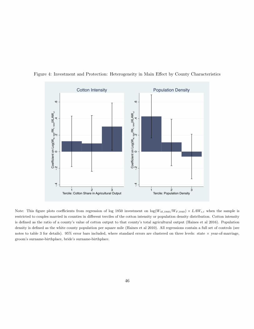
Figure 4: Investment and Protection: Heterogeneity in Main Effect by County Characteristics

-.4-.2

0.2

.4.6

Coef

ficie

nt o

n Lo

g(W

M, 1

840/W

F, 1

840)X

LAW

s,t

1 2 3Tercile: Cotton Share in Agricultural Output

Cotton Intensity

-.4-.2

0.2

.4.6

Coef

ficie

nt o

n Lo

g(W

M, 1

840/W

F, 1

840)X

LAW

s,t

1 2 3Tercile: Population Density

Population Density

Note: This figure plots coefficients from regression of log 1850 investment on log(WM,1840/WF,1840) × LAWs,t when the sample is

restricted to couples married in counties in different terciles of the cotton intensity or population density distribution. Cotton intensity

is defined as the ratio of a county’s value of cotton output to that county’s total agricultural output (Haines et al 2016). Population

density is defined as the white county population per square mile (Haines et al 2010). All regressions contain a full set of controls (see

notes to table 3 for details). 95% error bars included, where standard errors are clustered on three levels: state × year-of-marriage,

groom’s surname-birthplace, bride’s surname-birthplace.

46

Figure 5: Sensitivity to Omitting Common Names

02

46

810

1214

Sam

ple

size

(tho

usan

ds)

-.4-.2

0.2

.4.6

Coe

ffici

ent

0 10 20 30 40 50 60 70 80 90 100Maximum name frequency threshold

Coeff. on post law X log(Wm/Wf) Sample size

Note: Plots the OLS coefficient on LAWs,t × [logWi,1840 − logWj,1840], and 95% confidence intervals, using thespecification from Column (6) in Table 3. At each point, the coefficient and confidence interval are estimatedunder the restriction that neither the husband or wife has a name occurring more than the threshold indicated onthe horizontal axis. The sample size associated with each sample restriction is also plotted.

47

Table 1: Dates of Key Married Women’s Property Legislation in the 1840’sState Date Main Protection Wife’s Assets Ability to Sell

Law Change Wife’s Assets

Alabama Mar 1, 1848 All property owned at time of marriage, Wife cannot sellor acquired afterwards

Arkansas –Florida Mar 6, 1845 All property owned at time of marriage, Husband and wife can jointly

or acquired afterwards sell real estateGeorgia –Kentucky Feb 23, 1846 Real estate and slaves owned at time Husband and wife can jointly

of marriage, or acquired afterwards sell real estateLouisiana –Mississippi Feb 28, 1846 Real estate owned at time of marriage Husband and wife can jointly

and all other property required for the sell real estate; wife can sellmaintenance of the plantation (incl. individually if required forslaves) maintenance

North Jan 29, 1849 Husband’s interest in the wife’s real Wife’s real estate cannot beCarolina estate (i.e. profits or rents) not liable sold by husband without her

for his debts written consentTennessee Jan 10, 1850 Husband’s interest in the wife’s real Husband cannot sell his

estate (i.e. profits or rents) not liable interest is his wife’s realfor his debts estate

Texas –Virginia –

Notes: We omit Maryland and South Carolina from this Table as we do not have a sufficient number of marriage records to include

these states in our analysis. Due to their French and Spanish heritage, Louisiana and Texas had community property systems in place

that, by default, allowed men and women to have separate estates. Sources: Kahn (1996), Geddes and Lueck (2002), Warbasse (1987),

Kelly (1882), Wells (1878), Chused (1983) and Salmon (1982).

48

Table 2: Summary Statistics, Linked DataMean SD Min Max N

Panel A. Sample Restrictions

Husband & wife born in south 0.88 0.32 0 1 50809Household linkable to 1850 slave schedules 0.75 0.43 0 1 50809Resident in marriage state in 1850 0.77 0.42 0 1 50809Surname/birthplace matched to 1840 0.76 0.43 0 1 44949Meets all sample restrictions 0.39 0.49 0 1 50809

Panel B. Sample Characteristics

Husband’s age at marriage 26.99 8.82 15 91 19672Wife’s age at marriage 21.86 6.73 13 78 19672

Log total wealth, 1850 3.82 3.56 0 12.16 19672Fraction of wealth held in slaves 0.29 0.37 0 1 10980Nonzero slave wealth, 1850 0.24 0.43 0 1 19672Zero wealth in 1850 0.44 0.5 0 1 19672Employed in agriculture 0.67 0.47 0 1 19672

Married after law change 0.20 0.40 0 1 19672Resident in marriage county in 1850 0.71 0.45 0 1 19672

Groom’s 1840 log slave wealth 2.65 1.99 0 10.68 19672Bride’s 1840 log slave wealth 2.69 1.79 0 11.17 19672

Panel A documents what fraction of couples, for whom we linked the marriage and 1850 census records, satisfy the other sample

restrictions we impose (see Section 4 for details). Panel B presents summary statistics for our final sample

49

Table 3: Effect of Married Women’s Property Laws on 1850 Investment - OLS(1) (2) (3) (4) (5) (6)

Dep. var. log(Gross investment), 1850

Post Law -0.032 -0.029 -0.064 -0.062 -0.107 -0.104(0.101) (0.099) (0.098) (0.096) (0.121) (0.117)

Husband’s log(Wealth), 1840 0.176 0.179 0.177× Post Law (0.081)** (0.091)** (0.092)*Wife’s log(Wealth), 1840 -0.198 -0.178 -0.183× Post Law (0.090)** (0.086)** (0.088)**[Husband’s log(W) - Wife’s 0.236 0.227 0.227log(W), 1840] × Post Law (0.068)*** (0.068)*** (0.069)***

Adj-R2 0.095 0.095 0.197 0.197 0.198 0.198Obs 19672 19672 19672 19672 19672 19672

Age at marriage FE N N Y Y Y YBirthstate and literacy FE N N Y Y Y YFrequency names, bin FE N N Y Y Y YState specific lin. time trend N N N N Y Y

OLS estimates. All regressions contain state and year of marriage fixed effects, husband’s and wife’s 1840 wealth, and interactions

between premarital wealth variables and state and year of marriage fixed effects. Gross investment : value of household’s real estate and

slave holdings in 1850 census, gross of debt. Dependent variable: log(1+ Gross investment) . Husband’s/Wife’s 1840 wealth: average

log slave wealth (log(# slaves ×377 + 1)) of individuals with the same surname as the husband and wife in their respective states of

births in the 1840 census. Frequency names, bin FE : we calculate the relative prevalence of husband’s and wife’s family names per

state. We summarize this information in 10 bins, where bin 1 includes the rarest family names, and bin 10 the most common ones.

All (continuous) independent variables are normalized by their standard deviation; reported coefficients therefore indicate by what %

gross investment changes in response to a one standard deviation increase in the right hand side variable. All interactions with the

1840 wealth variables are in deviations from the mean. The coefficient on Post Law therefore measures the effect of the passage of a

Married Woman Property Act on a household with average wealth or average wealth difference. Standard errors (clustered at three

levels: state × year-of-marriage, groom’s surname-birthplace, bride’s surname-birthplace) are reported in parentheses: * p < 0.10, **p < 0.05, *** p < 0.01.

50

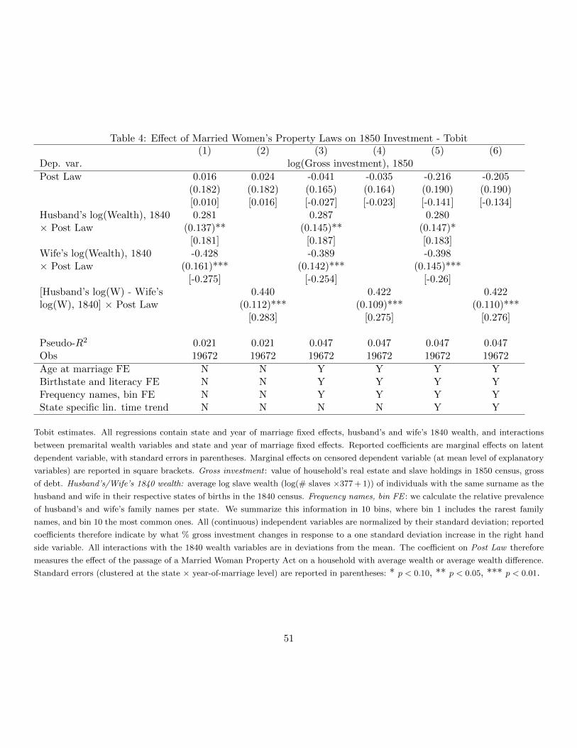
Table 4: Effect of Married Women’s Property Laws on 1850 Investment - Tobit(1) (2) (3) (4) (5) (6)

Dep. var. log(Gross investment), 1850

Post Law 0.016 0.024 -0.041 -0.035 -0.216 -0.205(0.182) (0.182) (0.165) (0.164) (0.190) (0.190)[0.010] [0.016] [-0.027] [-0.023] [-0.141] [-0.134]

Husband’s log(Wealth), 1840 0.281 0.287 0.280× Post Law (0.137)** (0.145)** (0.147)*

[0.181] [0.187] [0.183]Wife’s log(Wealth), 1840 -0.428 -0.389 -0.398× Post Law (0.161)*** (0.142)*** (0.145)***

[-0.275] [-0.254] [-0.26][Husband’s log(W) - Wife’s 0.440 0.422 0.422log(W), 1840] × Post Law (0.112)*** (0.109)*** (0.110)***

[0.283] [0.275] [0.276]

Pseudo-R2 0.021 0.021 0.047 0.047 0.047 0.047Obs 19672 19672 19672 19672 19672 19672

Age at marriage FE N N Y Y Y YBirthstate and literacy FE N N Y Y Y YFrequency names, bin FE N N Y Y Y YState specific lin. time trend N N N N Y Y

Tobit estimates. All regressions contain state and year of marriage fixed effects, husband’s and wife’s 1840 wealth, and interactions

between premarital wealth variables and state and year of marriage fixed effects. Reported coefficients are marginal effects on latent

dependent variable, with standard errors in parentheses. Marginal effects on censored dependent variable (at mean level of explanatory

variables) are reported in square brackets. Gross investment : value of household’s real estate and slave holdings in 1850 census, gross

of debt. Husband’s/Wife’s 1840 wealth: average log slave wealth (log(# slaves ×377 + 1)) of individuals with the same surname as the

husband and wife in their respective states of births in the 1840 census. Frequency names, bin FE : we calculate the relative prevalence

of husband’s and wife’s family names per state. We summarize this information in 10 bins, where bin 1 includes the rarest family

names, and bin 10 the most common ones. All (continuous) independent variables are normalized by their standard deviation; reported

coefficients therefore indicate by what % gross investment changes in response to a one standard deviation increase in the right hand

side variable. All interactions with the 1840 wealth variables are in deviations from the mean. The coefficient on Post Law therefore

measures the effect of the passage of a Married Woman Property Act on a household with average wealth or average wealth difference.

Standard errors (clustered at the state × year-of-marriage level) are reported in parentheses: * p < 0.10, ** p < 0.05, *** p < 0.01.

51

Table 5: Effect of Married Women’s Property Law on 1850 Investment – IV Estimates(1) (2) (3)

Dep. var log(Gross investment), 1850

Post Law -0.104 -0.544 -0.533(0.110) (0.121)*** (0.119)***

[Husband’s log(W) - Wife’s 0.227 0.126 0.117log(W), 1840] × Post Law (0.063)*** (0.069)* (0.068)*

F (Post Law) - 858.3 956.5F (Interaction) - 147.6 151.1Partial R2 (Post Law) - 0.695 0.729Partial R2 (Interaction) - 0.578 0.621Obs 19,672 19,672 19,672

Instruments = protection in:Wife’s birth st., marriage yr. N Y YMarriage st., yr. wife 22 N Y YHusband’s birth st., marriage yr. N N YMarriage st., yr. husband 27 N N Y

2SLS estimates. Column (1) repeats the OLS estimate from Table 3, Column (6). Remaining columns contain 2SLS estimates

instrumenting for Post Law and [Husband’s log(W) - Wife’s log(w)] × Post Law using the instruments indicated in the table, and the

instruments interacted with [Husband’s log(W) - Wife’s log(w)]. Gross investment : value of household’s real estate and slave holdings

in 1850 census, gross of debt. Dependent variable: log(1+ Gross investment) . Husband’s/Wife’s 1840 wealth: average log slave wealth

(log(# slaves ×377 + 1)) of individuals with the same surname as the husband and wife in their respective states of births in the 1840

census. All regressions include the full set of controls (see Table 3, Column 6), with the following exceptions: (1) we omit state of birth

fixed effects; (2) we omit controls for marriage year and we include linear and quadratic terms in the husband’s and wife’s age in 1850

instead of age fixed effects. All (continuous) independent variables are normalized by their standard deviation; reported coefficients

therefore indicate by what % gross investment changes in response to a one standard deviation increase in the right hand side variable.

All interactions with the 1840 wealth variables are in deviations from the mean. The coefficient on Post Law therefore measures the

effect of the passage of a Married Woman Property Act on a household with an average wealth difference. Standard errors (clustered

at the state × year-of-marriage level, or instrumented version thereof) are reported in parentheses: * p < 0.10, ** p < 0.05, ***p < 0.01.

52

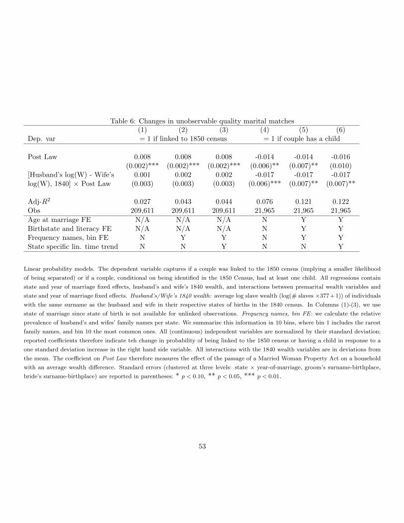
Table 6: Changes in unobservable quality marital matches(1) (2) (3) (4) (5) (6)

Dep. var = 1 if linked to 1850 census = 1 if couple has a child

Post Law 0.008 0.008 0.008 -0.014 -0.014 -0.016(0.002)*** (0.002)*** (0.002)*** (0.006)** (0.007)** (0.010)

[Husband’s log(W) - Wife’s 0.001 0.002 0.002 -0.017 -0.017 -0.017log(W), 1840] × Post Law (0.003) (0.003) (0.003) (0.006)*** (0.007)** (0.007)**

Adj-R2 0.027 0.043 0.044 0.076 0.121 0.122Obs 209,611 209,611 209,611 21,965 21,965 21,965

Age at marriage FE N/A N/A N/A N Y YBirthstate and literacy FE N/A N/A N/A N Y YFrequency names, bin FE N Y Y N Y YState specific lin. time trend N N Y N N Y

Linear probability models. The dependent variable captures if a couple was linked to the 1850 census (implying a smaller likelihood

of being separated) or if a couple, conditional on being identified in the 1850 Census, had at least one child. All regressions contain

state and year of marriage fixed effects, husband’s and wife’s 1840 wealth, and interactions between premarital wealth variables and

state and year of marriage fixed effects. Husband’s/Wife’s 1840 wealth: average log slave wealth (log(# slaves ×377+1)) of individuals

with the same surname as the husband and wife in their respective states of births in the 1840 census. In Columns (1)-(3), we use

state of marriage since state of birth is not available for unlinked observations. Frequency names, bin FE : we calculate the relative

prevalence of husband’s and wifes’ family names per state. We summarize this information in 10 bins, where bin 1 includes the rarest

family names, and bin 10 the most common ones. All (continuous) independent variables are normalized by their standard deviation;

reported coefficients therefore indicate teh change in probability of being linked to the 1850 census or having a child in response to a

one standard deviation increase in the right hand side variable. All interactions with the 1840 wealth variables are in deviations from

the mean. The coefficient on Post Law therefore measures the effect of the passage of a Married Woman Property Act on a household

with an average wealth difference. Standard errors (clustered at three levels: state × year-of-marriage, groom’s surname-birthplace,

bride’s surname-birthplace) are reported in parentheses: * p < 0.10, ** p < 0.05, *** p < 0.01.

53

Table 7: Effect of Married Women’s Property Laws on 1850 Gross Investment - Changing Bequest Behavior(1) (2) (3) (4) (5)

Dep. var. log(Gross Investment), 1850 log(Real log(SlaveEstate), 1850 Wealth), 1850

Post Law -0.041 -0.072 -0.097 -0.127 0.033(0.102) (0.100) (0.127) (0.111) (0.113)

Husband’s log(Wealth), 1840 0.158 0.165 0.162 0.102 0.127× Post Law (0.082)* (0.093)* (0.094)* (0.076) (0.085)Wife’s log(Wealth), 1840 -0.219 -0.197 -0.204 -0.109 0.003× Post Law (0.093)** (0.090)** (0.092)** (0.071) (0.087)% Children male, 1840, wife -0.033 -0.062 -0.062× Wife’s log(Wealth) (0.109) (0.102) (0.101)× × Post Law 0.117 0.090 0.087

(0.045)*** (0.049)* (0.049)*% Children male, 1840, wife -0.153 -0.151 -0.150

(0.087)* (0.092)* (0.093)% Children male, 1840, wife -0.030 -0.013 -0.013× Post Law (0.076) (0.075) (0.076)

Adj-R2 / Pseudo-R2 0.096 0.199 0.200 0.157 0.188Obs 19541 19541 19541 27090 19672

Age at marriage FE N Y Y Y YBirthstate and literacy FE N Y Y Y YFrequency names, bin FE N Y Y Y YState specific lin. time trend N N Y Y Y

OLS estimates. All regressions contain state and year of marriage fixed effects, husband’s and wife’s 1840 wealth, and interactions

between all included 1840 variables and state and year of marriage fixed effects. Gross investment : value of household’s real estate

and slave holdings in 1850 census, gross of debt. When estimating OLS the dependent variable is log(1+ Gross investment). Hus-

band’s/Wife’s 1840 wealth: average log slave wealth (log(# slaves ×377 + 1)) of individuals with the same surname as the husband

and wife in their respective states of births in the 1840 census. % Children male, 1840, wife: percentage of children that are male in

households with the same surname as the wife in her state of birth in the 1840 census. Frequency names, bin FE : we calculate the

relative prevalence of husband’s and wife’s family names per state. We summarize this information in 10 bins, where bin 1 includes

the rarest family names, and bin 10 the most common ones. All (continuous) independent variables are normalized by their standard

deviation; reported coefficients therefore indicate by what % gross investment changes in response to a one standard deviation increase

in the right hand side variable. All interactions with the 1840 wealth variables are in deviations from the mean. The coefficient on

Post Law therefore measures the effect of the passage of a Married Woman Property Act on a household with an average wealth dif-

ference. Standard errors (clustered at three levels: state × year-of-marriage, groom’s surname-birthplace, bride’s surname-birthplace)

are reported in parentheses: * p < 0.10, ** p < 0.05, *** p < 0.01.

54

Table 8: Effect of Married Women’s Property Laws on 1850 Gross Investment - Exemption levels and MacroConditions

(1) (2) (3) (4) (5) (6)Dep. var. log (Gross Investment), 1850

Post Law -0.034 -0.068 -0.112 -0.005 -0.191 -0.036(0.099) (0.095) (0.117) (0.125) (0.135) (0.143)

[Husband’s log(W) - Wife’s 0.236 0.227 0.226 0.221 0.228 0.221log(W), 1840] × Post Law (0.068)*** (0.069)*** (0.069)*** (0.069)*** (0.073)*** (0.072)***State exemption level -0.001 -0.001 -0.002

(0.000)*** (0.000)*** (0.000)***× [Husband’s log(W) 0.000 0.000 0.000

- Wife’s log(W), 1840] (0.000) (0.000) (0.000)

Adj-R2 0.095 0.198 0.198 0.196 0.199 0.197Obs 19672 19672 19672 19372 19672 19372

Age at marriage FE N Y Y N Y YBirthstate and literacy FE N Y Y N Y YFrequency names, bin FE N Y Y N Y YState specific lin. time trend N N Y N N Y

1840 Cotton & SlaveIntensity × Year FEs N N N Y N YAnnual Cotton & SlavePrices × State FEs N N N N Y Y

OLS estimates. All regressions contain state and year of marriage fixed effects, husband’s and wife’s 1840 log wealth, and interactions

between premarital wealth variables and state and year of marriage fixed effects. Gross investment : value of household’s real estate

and slave holdings in 1850 census, gross of debt. The dependent variable is log (1+ Gross investment). Husband’s/Wife’s 1840 wealth:

average log slave wealth (log(# slaves ×377+1)) of individuals with the same surname as the husband and wife in their respective states

of births in the 1840 census. State exemption level : $ amount exempt in case of insolvency. Cotton & slave prices: price per pound raw

cotton; average price per slave; from HSUS. Cotton & slave intensity : pounds of cotton picked per white population in 1840, state level;

number of slaves per white population, state level; from Haines & ICPSR Frequency names, bin FE : we calculate the relative prevalence

of husband’s and wife’s family names per state. We summarize this information in 10 bins, where bin 1 includes the rarest family

names, and bin 10 the most common ones. All (continuous) independent variables are normalized by their standard deviation; reported

coefficients therefore indicate by what % gross investment changes in response to a one standard deviation increase in the right hand

side variable. All interactions with the 1840 wealth variables are in deviations from the mean. The coefficient on Post Law therefore

measures the effect of the passage of a Married Woman Property Act on a household with an average wealth difference. Standard

errors (clustered at three levels: state × year-of-marriage, groom’s surname-birthplace, bride’s surname-birthplace) are reported in

parentheses: * p < 0.10, ** p < 0.05, *** p < 0.01.

55

APPENDICES FOR ONLINE PUBLICATION ONLY

A Theory Appendix

A.1 Proofs: Main Model

Proof. Proposition 1:The household solves the following problem:

maxc0,e,ρg ,ρb

log c0 +1

2θ[logR(w − c0 + e)− ρge

]+

1

2θ [logR(w − c0 + e)− ρb] e

− λ(2− ρg − ρb) (2)

− µ[ρge− (R− β∆r)(w − c0 + e)

](3)

− χ(−e)

The first order conditions are:

c0 :1

c0−

12θR

R(w − c0 + e)− ρge−

12θR

R(w − c0 + e)− ρbe− µ(R− β∆r) = 0

e :12θ(R− ρg)

R(w − c0 + e)− ρge+

12θ(R− ρb)

R(w − c0 + e)− ρbe− µ(ρg −R+ β∆r) + χ = 0

ρg :−1

2θe

R(w − c0 + e)− ρge+ λ− µe = 0

ρb :−1

2θe

R(w − c0 + e)− ρbe+ λ = 0

Case 1: IC contstraint is slack (β < r−1∆r )

From the F.O.C.’s for ρg and ρb, we obtain the following:

µ =1

2θ

[1

R(w − c0 + e)− ρbe− 1

R(w − c0 + e)− ρge

](4)

Suppose that the incentive compatibility constraint is slack, so µ = 0. Then, expression (4)implies that:

R(w − c0 + e)− ρbe = R(w − c0 + e)− ρgeOr, consumption is equalized in both states of the world. Then, from the F.O.C.’s for ρg andρb, and imposing the constraint that ρb = 2− ρg, we get the following:

R(w − c0 + e)− ρge = R(w − c0 + e)− (2− ρg)e

⇒ ρg = 1 +∆r

2+

∆r(w − c0)

2e

Now, substituting all of this into the expression for ∂U/∂e (and assuming that the e > 0constraint is slack, so χ = 0), we find the following:

∂U

∂e=

12θ

R(w − c0 + e)− ρge(R− ρg +R− 2 + ρg)

=12θ

R(w − c0 + e)− ρge(R+R− 2) > 0 (5)

56

So, the household will want to borrow e = ∞, which is intuitive, as it is able to smoothconsumption across states and the project has positive expected returns. Next, we checkwhen this e and ρg will satisfy the incentive compatibility constraint so that µ = 0:

R(w − c0 + e)− ρge− β∆r(w − c0 + e) > 0

⇒ R(w − c0)

e+R− 1− ∆r

2− ∆r(w − c0)

2e− β∆r(w − c0)

e− β∆r > 0

Letting e go to ∞, we arrive at

R− 1− ∆r

2− β∆r = r − 1− β∆r > 0

This will hold iff β < r−1∆r .

Case 2: IC constraint is binding - outside investment is infinite ( r−1∆r < β < 2r−2

∆r )

Now suppose that µ > 0. Substituting expression (4) for µ, the constraint that ρg + ρb = 2,and the incentive compatibility constraint (3) into the F.O.C. for e, we get the following (aftersome algebra):

∂U

∂e=

12θ

w − c0 + e−

12θ(β∆r − 2(r − 1))

(2r − β∆r)(w − c0 + e)− 2e+ χ

=θ

C[(2r − 1− β∆r)(w − c0) + e(2r − 2− β∆r)] + χ (6)

Here, C ≡ (w − c0 + e) [(2r − β∆r)(w − c0 + e)− 2e] > 0, as this multiplies consumption inthe good and bad states of the world, which must both be greater than zero. In addition,β∆r < 2r− 1. To see this, note that, by assumption, β < 1. In addition, the restriction thatR > 1

2−1/R > 12 guarantees that 2r−1

∆r > 1, since

2r − 1

∆r=R+R− 1

R−R>R− 1/2

R− 1/2= 1 (7)

Expression (6) therefore implies that if β∆r < 2r − 2, then ∂U/∂e > 0∀e, so the householdwill want to borrow an infinite amount. Because the incentive compatibility constraint holdswith equality, this implies the following equilibrium value of ρg:

ρge = (R− β∆r)(w − c0) + (R− β∆r)e

⇒ρg = (R− β∆r)w − c0

e+R− β∆r → R− β∆r (8)

So, if r−1∆r < β < 2r−2

∆r , the household will borrow an infinite amount but will be constrainedin the ρg it can select by the incentive compatibility constraint.

Case 3: IC constraint is binding - outside investment is limited (β > 2r−2∆r )

When β > 2r−2∆r , the F.O.C. for e is satisfied when

e =2r − 1− β∆r

2− 2r + β∆r(w − c0) > 0

and χ = 0. So, the household will take on a non-zero, non-infinite loan of exactly this size ifβ is the range specified in the proposition.

Substituting the solution for e, the above expression for µ, and the constraint that ρg + ρb =2 into the F.O.C. for c0, we get c∗0 = 1

1+θw, which gives us the expression for e∗ in theproposition. Substituting all of this into the F.O.C. for ρg, we get the ρg in the proposition.

57

Proof. Proposition 2:With incomplete markets, it is clear that the household will choose a risk-free loan, as a risky

loan would leave it with zero consumption in the bad state of the world and U = −∞, So, thehousehold’s maximization problem can be written as follows:

maxc0,l

log c0 +1

2θ log

[R(w − c0 + l)− l

]+

1

2θ log [R(w − c0 + l)− l]

The first order conditions are:

c0 :1

c0−

θ2R

R(w − c0 + l)− l−

θ2R

R(w − c0 + l)− l= 0

l :θ2(R− 1)

R(w − c0 + l)− l+

θ2(R− 1)

R(w − c0 + l)− l= 0

After some algebra, the FOC for l simplifies to the following:

l =RR− r

(R− 1)(R− 1)(w − c0) (9)

Notice that, for the household to be willing to take on a positive amount of debt, returns on therisky project must be such that RR > r. This is guaranteed by the assumption that

R >1

2− 1/R.

Substituting this expression into the FOC for c0 we arrive at c0 = w1+θ . Substituting this into the

above expression for l, we get the expression for l∗ in the proposition.

Notice that this always satisfies the incentive compatibility constraint:

R(w − c0 + l)− l > β∆r(w − c0 + l) (10)

First, notice that l < R(w − c0 + l):

R(w − c0 + l)− l =R(r − 1)

(R− 1)(1−R)− RR− r

(R− 1)(1−R)=

(1−R)(R−R)

2(R− 1)(1−R)> 0

So,

R(w − c0 + l)− l > R(w − c0 + l)−R(w − c0 + l) = ∆r(w − c0 + l) > β∆r(w − c0 + l)

Proof. Lemma 3:We only need to prove that e∗ > l∗, since c∗0 is the same under complete and incomplete

contracts. From Propositions 1 and 2:

e∗ =

(θ

1 + θ

)2r − 1− β∆r

β∆r − 2(r − 1)w

l∗ =

(θ

1 + θ

)RR− r

(R− 1)(1−R)w

58

So, we need to show that the following holds for all β ∈ [2r−2∆r , 1]:

2r − 1− β∆r

β∆r − 2(r − 1)>

RR− r(R− 1)(1−R)

(11)

First, recall from expression (7) that β∆r < 2r − 1. Second, notice the left hand side of theinequality we are trying to prove is strictly decreasing in β, as the numerator is strictly decreasingin β and the denominator is strictly increasing in β. So, if the following inequality holds, this provesthe proposition:

2r − 1−∆r

∆r − 2r + 1− RR− r

(1−R)(R− 1)> 0

After some algebra, the left hand side of this inequality simplifies to:

1−R2(1−R)(R− 1)

> 0

So, borrowing always increases under complete markets relative to incomplete markets with noprotection. This result is self evident when β < 2r−2

∆r , since in this case borrowing under completemarkets is infinite.Proof. Proposition 4:

Under incomplete contracts with protection, the household has three options: (1) contract arisk-free loan; (2) contract a risky loan; (3) do not borrow. If the household opts for a risk-freeloan, it will solve a maximization problem similar to that in Proposition 2, subject to the additionalconstraint that (1−R)l ≤ R(wM − c0). If the household opts for a risky loan, it will borrow morethan R

1−R(wM − c0) and the lender will not be able to recover the full amount of his loan in the badstate of the world. In response, he will charge a risk premium ρ that satisfies the following zeroprofit condition:

R(wM − c0 + l) + ρl = 2l (12)

To support risky lending, the borrower’s incentives must always be compatible with repayment ofthe loan in the good state of the world:

R(wM − c0 + l)− ρl ≥ β∆r(wM − c0 + l) (13)

Case 1: wM/wF < φ1

We first consider the case in which households want to consume more than wM at t = 0.In this case, the household consumes of all of its pledgeable collateral, and the incentivecompatibility constraint will never be satisfied for a loan that offers the lender a risk-free rateof return, so l = 0. To see this, combine (12) and (13) and set wM − c0 = 0 to notice that

(R− β∆r)l − (2−R)l <[R− (2r − 2)

]l − (2−R)l = 0

With no borrowing, the household’s problem simplifies to:

maxc0

log c0 +1

2θ log

[R(wM + wF − c0)

]+

1

2θ log [R(wM + wF − c0)]

We solve this problem and check when wM − c0 ≤ 0. The first order condition is:

1

c0−

12θR

(R(wM + wF − c0))−

12θR

(R(wM + wF − c0))

59

The solution is:

c0 =1

1 + θ(wM + wF ) (14)

Such a solution is only consistent with zero borrowing if wM − c0 ≤ 0, or if wMwF≤ 1

θ . Next,we solve the household’s problem under the constraint that borrowing is weakly positive, andwe will verify that, at the point where borrowing is exactly reduced to zero, wM

wF< 1

θ .

Case 2: φ1 < wM/wF < φ2

Here, we consider the case in which wM − c0 > 0, so borrowing is possible, and consumptionin the bad state of the world is simply RwF . The household maximizes utility subject tothe lenders’ zero profit condition (12), and the household’s incentive compatibility constraint(13):

maxc0,l,ρ

log c0 +1

2θ log

[R(wM + wF − c0 + l)− ρl

]+

1

2θ log [R(wF )]

− λ(2l − ρl −R(wM − c0 + l)) (15)

− µ[ρl − (R− β∆r)(wM − c0 + l)

](16)

− χ(−l)

The first order conditions are:

c0 :1

c0−

12θR

R(wM + wF − c0 + l)− ρl− µ(R− β∆r) = 0

l :12θ(R− ρ)

R(wM + wF − c0 + l)− ρl− µ(ρ−R+ β∆r) + χ = 0

ρ :−1

2θl

R(wM + wF − c0 + l)− ρl+ λ− µl = 0

We first prove that the IC constraint (16) always binds. Suppose it is slack and µ = 0. Then,imposing that the lender’s zero profit condition (15) holds with equality, the F.O.C. for lwould be the following:

12θ[R− (2−R− wM−c0

l R)]

R(wM + wF − c0 + l)− l+ χ = 0

Because R + R > 2 and χ ≥ 0, this will never hold. So, it must be the case that the ICconstraint (16) holds with equality.

Given that both the IC constraint and (15) need to hold with equality, the solution for theoptimal loan size is given by:

(R− β∆r)(wM − c0 + l) = ρl = 2l −R(wM − c0 + l)

⇒ l =2r − β∆r

2− 2r + β∆r(wM − c0) (17)

Given this, consumption in the good state of the world simplifies to:

R(wM − c0 + l)− ρl =2β∆r

2− 2r + β∆r(wM − c0) +RwF

60

and we can rewrite the problem in the following way:

maxc0

log c0 +θ

2log

[2β∆r

2− 2r + β∆r(wM − c0) +RwF

]+θ

2log(RwF )

For simplicity, define ψ ≡ 2β∆r2−2r+β∆r . Then we can write the F.O.C. for c0 as follows:

1

c0−

θ2ψ

ψ(wM − c0) +RwF= 0

This determines optimal consumption in t = 0:

c0 =

(2

2 + θ

){wM +

R

ψwF

}=

(2

2 + θ

){wM +

R(2− 2r + β∆r)

2β∆rwF

}(18)

The expressions for l and total investment in the proposition follow directly from expressions(17) and (18).

Next, we check whether wM − c0 > 0. This is true iff

θ

2 + θwM −

(2

2 + θ

)R(2− 2r + β∆r)

2β∆rwF > 0⇒ wM

wF>R(2− 2r + β∆r)

θβ∆r

We verify that this cutoff is compatible with our findings from Case 1. In particular, we

need wMwF≤ 1

θ for all wMwF≤ R(2−2r+β∆r)

θβ∆r . Notice that R(2−2r+β∆r)β∆r < 1, which implies that

R(2−2r+β∆r)θβ∆r < 1

θ :

R(2− 2r + β∆r)

β∆r− 1 =

1

∆r

[R(2− 2r + β∆r)

β−∆r

]=

1

∆r

[−R(2− 2r)

β+R∆r −∆r

]<

1

∆r(−R(2− 2r) +R∆r −∆r) =

1

∆r(R+R− 2RR)

=2

∆r(r −RR) < 0 (19)

Thus, zero borrowing is certainly preferable to risky borrowing when wMwF≤ R(2−2r+β∆r)

θβ∆r , and

zero borrowing may be preferable to risky borrowing when wMwF

< 1θ . So, the household will

switch from no borrowing to risky borrowing when

wM/wF = φ1 ∈(R(2− 2r + β∆r)

θβ∆r,1

θ

). (20)

Case 3: wM/wF > φ2

Next, we consider the case in which a risk-free loan is optimal with protection. We first needto derive when a risk-free loan is attainable. This is the case when the optimal loan size fromProposition 2 (no protection) is risk-free even when returns associated with wF are protected:(

θ

1 + θ

)RR− r

(R− 1)(1−R)(wM + wF ) ≤ R

1−R

{θ

1 + θwM −

1

1 + θwF

}(21)

61

This is true iff:wMwF≥

2[R− 1 + θ(RR− r)

]θ∆r

= φ2

(22)

We know that, as wF → 0, a risk free loan is preferable, since utility in the bad state ofthe world with a risky loan approaches −∞. So, there exists some φ2 ≥ φ

2such that the

household will choose the no-protection optimum when wM/wF > φ2.

Risky borrowing always takes place for some part of the wM/wF distribution; that is φ2 > φ1.Using expressions (20) and (22), this is the case iff

φ2 ≥2[R− 1 + θ(RR− r)

]θ∆r

>1

θ≥ φ1

It is sufficient to show that 2(R−1)∆r − 1 > 0:

2(R− 1)

∆r− 1 =

1

∆r(2R− 2−R+R)

=1

∆r(2r − 2) > 0

Finally, we show that φ2 > φ2. To do this, we will show that household strictly prefers a

risky loan to a risk-free loan when wM/wF = φ2.

Expressions (21) and (22) indicate that, when wMwF

= φ2, the optimal risk free loan size is

l∗ =R

1−R(wM − c∗0) (23)

After loan repayment, consumption in the bad state equals c∗1,B = RwF . This is identical toconsumption in the bad state when the household contracts a risky loan (c1,B).

Now, consider the household’s consumption and investment decision when the householdcontracts a risky loan. Suppose that the household were to select c0 = c∗0, so that consumptionat t = 0 and consumption in the bad state are identical to a risk-free loan. If the householdis able to increase consumption in the good state (c1,G), holding c∗0 and c1,B constant, then itfollows that the household is certainly better off contracting a risky loan. The largest loan thehousehold will be able to contract (while satisfying the lender’s zero profit condition and theborrower’s incentive compatibility constraint) is pinned down by the following two equations:

ρl +R(wM − c∗0 + l) = 2l (24)

R(wM − c∗0 + l)− ρl = β∆r(wM − c∗0 + l) (25)

After some algebra, this implies the following maximum loan size:

l =2r − β∆r

2− 2r + β∆r(wM − c∗0) (26)

Thus, consumption in the good state with this loan size would be:

c1,G = R(wM + wF − c∗0 + l)− ρl

= RwF +2β∆r

2− 2r + β∆r(wM − c∗0) (27)

62

This follows from substituting in the solutions for l and ρl from (24) and (26) and simplifying.

Consumption in the good state with a risk-free loan is:

c∗1,G = R(wM + wF − c∗0 + l∗)− l∗ = RwF +∆r

1−R(wM − c∗0) (28)

This follows from substituting l∗ from (23) and simplifying.

So, the household can increase consumption in the good state iff:

c1,G − c∗1,G > 0

⇒ 2β∆r

2− 2r + β∆r− ∆r

1−R> 0

⇒ (1− β)(2r − 2)

(2− 2r + β∆r)(1−R)> 0

Since r > 1 and β < 1, this is always true.

Thus, when wM/wF = φ2, it can achieve c0 = c∗0, c1,B = c∗1,B, and c1,G > c∗1,G by contracting

a risky loan. This means that the household is unambiguously better off contracting a riskyloan, which implies that φ2 > φ

2.

Proof. Lemma 5a:In the case with no protection, we obtain the following elasticities of investment with respect

to wM and wF :

ε∗M =∂I∗

∂wM

wMI∗

=

(r − 1

(R− 1)(1−R)

)(θ

1 + θwM

)[(r − 1

(R− 1)(1−R)

)(θ

1 + θ

)(wM + wF )

]−1

=wM

wM + wF

ε∗F =∂I∗

∂wF

wFI∗

=

(r − 1

(R− 1)(1−R)

)(θ

1 + θwF

)[(r − 1

(R− 1)(1−R)

)(θ

1 + θ

)(wM + wF )

]−1

=wF

wM + wF

Case 1: wM/wF < φ1 or wM/wF > φ2

If wM/wF < φ1, then I = θ1+θ (wM + wF ), so εM = wM

wM+wF= ε∗M and εF = wF

wM+wF= ε∗F , by

a similar argument to the one made for the no protection case. If wM/wF > φ2, then I = I∗,so εM = ε∗M and εF = ε∗F . So, the proposition holds in these cases.

Case 2: φ1 ≤ wM/wF ≤ φ2

In this case, I takes the form χMwM + χFwM , where

χM ≡(

θ

2 + θ

)2

2− 2r + β∆r(29)

63

and

χF ≡ 1−(

2

2 + θ

)R

β∆r. (30)

Then:

εM =χMwM

χMwM + χFwF

εF =χFwF

χMwM + χFwF

The difference between εM and ε∗M is:

εM − ε∗M =χMwM

χMwM + χFwF− wMwM + wF

=wMwF (χM − χF )

(wM + wF )(χMwM + χFwF )(31)

This is positive if χM > χF . By a similar argument, εF −ε∗F < 0 if χM > χF . So, if χM > χF ,this proves the proposition.

After some algebra, we arrive at the following:

χM − χF =1

β∆r(2 + θ)

[(2

2− 2r + β∆r− 1

)θβ∆r + 2(R− β∆r)

](32)

Now, R − β∆r > 0. So, if 22−2r+β∆r > 1, then χM − χF > 0. To show that this is the case,

we show that 2− 2r + β∆r < 1.

2− 2r + β∆r < 2− 2r + ∆r = 2(1−R) < 2(1− 1

2) = 1

This follows from the restriction we made earlier that β < 1 and R > 12 .

Proof. Lemma 5b:

Case 1: wM/wF < φ1 or wM/wF > φ2

Notice that I − I∗ < 0 when wM/wF < φ1. And, I − I∗ = 0 ≥ 0 when wM/wF > φ2.

Case 2: φ1 < wM/wF < φ2

The proof proceeds by characterizing the cutoff φ∗ such that I∗ − I < 0 if wMwF

< φ∗ and

I∗ − I > 0 if φ∗ ≤ wMwF

< φ2. We procede in two steps:

(a) We first calculate the level of wMwF

where I∗ − I = 0. First, recall that I∗ takes the formχIC(wM + wF ), where

χIC ≡(

θ

1 + θ

)r − 1

(R− 1)(1−R). (33)

And, recall from the proof of Lemma 5a that when φ1 < wM/wF < φ2, I takes the formχMwM + χFwF , where χM and χF are given by (29) and (30). Then,

I∗ − I = (χIC − χM )wM + (χIC − χF )wF

64

This only has a solution if χM > χIC and χIC > χF ; this follows from the fact thatχM > χF , which we proved in Lemma 5a.

We first show that χM > χIC :

χM−χIC =2θ

(2 + θ)(2− 2r + β∆r)− θ(r − 1)

(1 + θ)(R− 1)(1−R)>

θ

2− 2r + β∆r

(2

2 + θ− 1

1 + θ

)

This follows from the fact that investment under incomplete markets(

θ(r−1)

(1+θ)(R−1)(1−R)(wM+

wF ))

is smaller than investment under complete markets(

θ2−2r+β∆r (wM + wF )

). So,

χM − χIC >θ

2− 2r + β∆r

(θ

(1 + θ)(2 + θ)

)> 0

Next, we show that χIC > χF . Consider expression (30) for χF . Since 22+θ >

11+θ and

R > β∆r, it must be that χF < θ1+θ . From expression (33) for χIC it is clear to see

that, because r−1(R−1)(1−R)

> 1, χIC >θ

1+θ . From here it follows that χIC > χF .

These results indicate that there exists a φ∗∗ such that

I − I∗ = 0⇒ wMwF

=χIC − χFχM − χIC

≡ φ∗∗ (34)

(b) We now prove thatφ∗ = max{φ∗∗, φ1}

If φ1 < φ∗∗, then φ∗∗ satisfies the condition for φ∗ stated in the proposition. However,if φ∗∗ ≤ φ1, then I − I∗ > 0 ∀ wM/wF ∈ [φ1, φ2], and φ1 satisfies the condition for φ∗

stated in the proposition.

The only thing left to show is that φ∗∗ < φ2. To do this, we use the result from Proposi-tion 4 that φ

2< φ2, where φ

2is defined in expression (22), and we will show that I > I∗

when wMwF

= φ2, indicating that φ∗∗ < φ

2< φ2.

Because the interest rate paid on l in the good state will be greater than the interestrate paid on l∗ in the good state (since l is risky and l∗ is not), it is sufficient to showthat consumption in the good state with protection (c1,G) is greater than consumptionin the good state without protection (c∗1,G) for wM/wF = φ

2.

Given the solutions for c∗0 and l∗, we know that households will optimally select thefollowing ratio of c∗1,G to c∗0:

c∗1,Gc∗0

=θ

2

(∆r

1−R

)(35)

And, from Proposition 4, we know that when φ1 < wM/wF < φ2, households willoptimally select the following ratio of c1,G to c0:

c1,G

c0=θ

2

(2β∆r

2− 2r + β∆r

)(36)

65

In the proof of Proposition 4, we show that 2β∆r2−2r+β∆r −

∆r1−R > 0, which means that

c1,Gc0

>c∗1,Gc∗0

.

Now, suppose that c1,G < c∗1,G when wM/wF = φ2. Because

c1,Gc0

>c∗1,Gc∗0

, this would imply

that c0 < c∗0. According to the proof of Proposition 4, this would leave the householdstrictly worse off with protection because c1,B = c∗1,B . As a result, the household can bemade strictly better off with protection. Thus, we know that c1,G > c∗1,G, which means

that I > I∗ when wM/wF = φ2. This implies that φ∗∗ < φ2.

A.2 Model of Changing Spousal Bargaining Power

We write down a simple, two period model, in which parents have preferences over their ownconsumption and their children’s consumption. Parents produce output using labor and physicalcapital, and they split their time between labor and investing in children’s human capital. Parentsthen transfer a portion of the output they produce to their children, which forms the capital inputin children’s production function. This is a simplified and slightly modified version of the modelpresented in Doepke and Tertilt (2009).

Each couple has one child, and the husband and wife have different preferences over own con-sumption and the child’s consumption:

Ui = log c0 + θi log c1

Here, i ∈ {M,F} indexes gender, and θF > θM .A couple is endowed with a certain level of human capital, H0, and physical capital, W0. In

addition, the couple has a time allocation of 1, and must choose a quantity of time, t ≤ 1, to devoteto producing output, Q0. The remaining time, 1 − t, is devoted to investing in the child’s humancapital. The output a couple produces with a given input of labour and capital is given by thefollowing Cobb-Douglas production function:

Q0 = A(tH0)αW 1−α0

where α < 1. The couple consumes a portion c0 of Q0, and transfers the remainder, W1 = Q0− c0,to its child; this forms the capital input in the child’s production function. As this is a two periodmodel, the child devotes all of his or her time to labor and consumes all the output:

c1 = A(H1)α(W1)1−α

The child’s human capital depends on the parents’ human capital, as well as the time the parentsspend investing in the child’s education, in the following way:

H1 = (1− t)ψH0

Let β represent the relative bargaining power of the wife, so the couple chooses t and W1 tomaximize the following utility function (subject to constraints):

U = (1− β)UM + βUF = log c0 +(

(1− β)θM + βθF

)log c1

66

We denote θ ≡ (1 − β)θM + βθF . We assume that θF > θM , and that the passage of a marriedwomen’s property act leads to an increase in β; thus, the passage of a property act generates anincrease in θ. This directly follows Doepke and Tertilt (2009). We solve for optimal t and W1 fora generic θ, then look at how t∗ and W ∗1 respond to an increase in θ.

Given the constraints enumerated above, the couple solves the following problem:

maxt,W1

log(A(tH0)αW 1−α

0 −W1

)+ θ log

(A((1− t)ψH0

)αW 1−α

1

)After some algebra, the first order conditions for t and W1 simplify to the following:

t :Q0

t(Q0 −W1)=

θψ

1− t

W1 : W1 =θ(1− α)

1 + θ(1− α)Q0

Substituting the FOC for W1 into the FOC for t, we obtain the following:

Q0

t(

11+θ(1−α)

)Q0

=θψ

1− t⇒ t∗ =

1 + θ(1− α)

θψ + 1 + θ(1− α)

So, the couple will devote a fraction of its time to labor, which depends on the weight the coupleplaces on children’s consumption (θ), the labor share in output (α), and the return on investingin children’s human capital (ψ). It is straightforward to show that the amount of time the couplespends on labor is decreasing in θ:

∂t

∂θ=

−ψ(θψ + 1 + θ(1− α)

)2 < 0

This implies that the amount of output the couple produces, Q0, is declining in θ:

∂Q0

∂θ= (AHα

0 W1−α0 )αtα−1 ∂t

∂θ< 0

What happens to the transfer a couple makes to its child? Substituting the expression for t∗

into the FOC for W1, we get the following:

W ∗1 =

(θ(1− α)

1 + θ(1− α)

)(1 + θ(1− α)

θψ + 1 + θ(1− α)

)αAHα

0 W1−α0

Define the following functions of θ:

f(θ) ≡ θ(1− α)

1 + θ(1− α)

g(θ) ≡ 1 + θ(1− α)

θψ + 1 + θ(1− α)

Then, ∂W ∗1 /∂θ will be directly proportional to the following:

f ′(θ)g(θ)α + αf(θ)g(θ)α−1g′(θ) = g(θ)α−1(f ′(θ)g(θ) + αf(θ)g′(θ)

)

67

Note the following solutions for f ′ and g′:

f ′(θ) =1− α(

1 + θ(1− α))2

g′(θ) =−ψ(

θψ + 1 + θ(1− α))2

Thus, after some algebra, we arrive at the following:

f ′(θ)g(θ) + αf(θ)g′(θ) =1− α(

1 + θ(1− α))(θψ + 1 + θ(1− α)

)(1− αθψ

θψ + 1 + θ(1− α)

)

This is clearly positive, as α < 1. So, we conclude that W1 is increasing in θ.To summarize, if married women’s property rights increase women’s bargaining power, and

women place more weight on their children’s consumption than men, we should expect the passageof a property law to: (i) decrease the amount of output a couple produces; (ii) increase output netof current consumption, or the size of the transfer a couple makes to its children.

B Data Appendix

1850 Census

We use the full count 1850 Federal Census from the North Atlantic Population Project (NAPP).

This dataset is largely clean; however, the 1850 census does not identify married couples, so we

need to assign marital status to individuals based on their placement in the household. We apply

a rule that is very similar to the rule that IPUMS uses: we define a married couple to be a man

(15+) and a woman (13+) with the same surname, entered adjacent to one another in the census

manuscript, with the man no more than 25 years older or less than 10 years younger than the

woman. We also eliminate potential siblings, defined as being part of a descending list of similarly

aged individuals with the same surname. We test our assignment rule by verifying that it broadly

assigns the same marital status to couples in the 1850 1% samples as the IPUMS procedure: our

procedure and the IPUMS procedure assign the same marital status to 97% of southern women in

the 1850 1% sample.

The 1850 population census contains information about the total value of real estate that a

household owned. Enumerators were instructed to “insert the value of real estate owned by each

individual enumerated; you are to obtain the value of real estate by inquiry of each individual who

is supposed to own real estate, be the same located where it may, and insert the amount in dollars;

no abatement of the value is to be made on account of any lien or incumbrance [sic] thereon in the

nature of debt.”(Ruggles et al 2010). Real estate included both land and buildings. At the time,

68

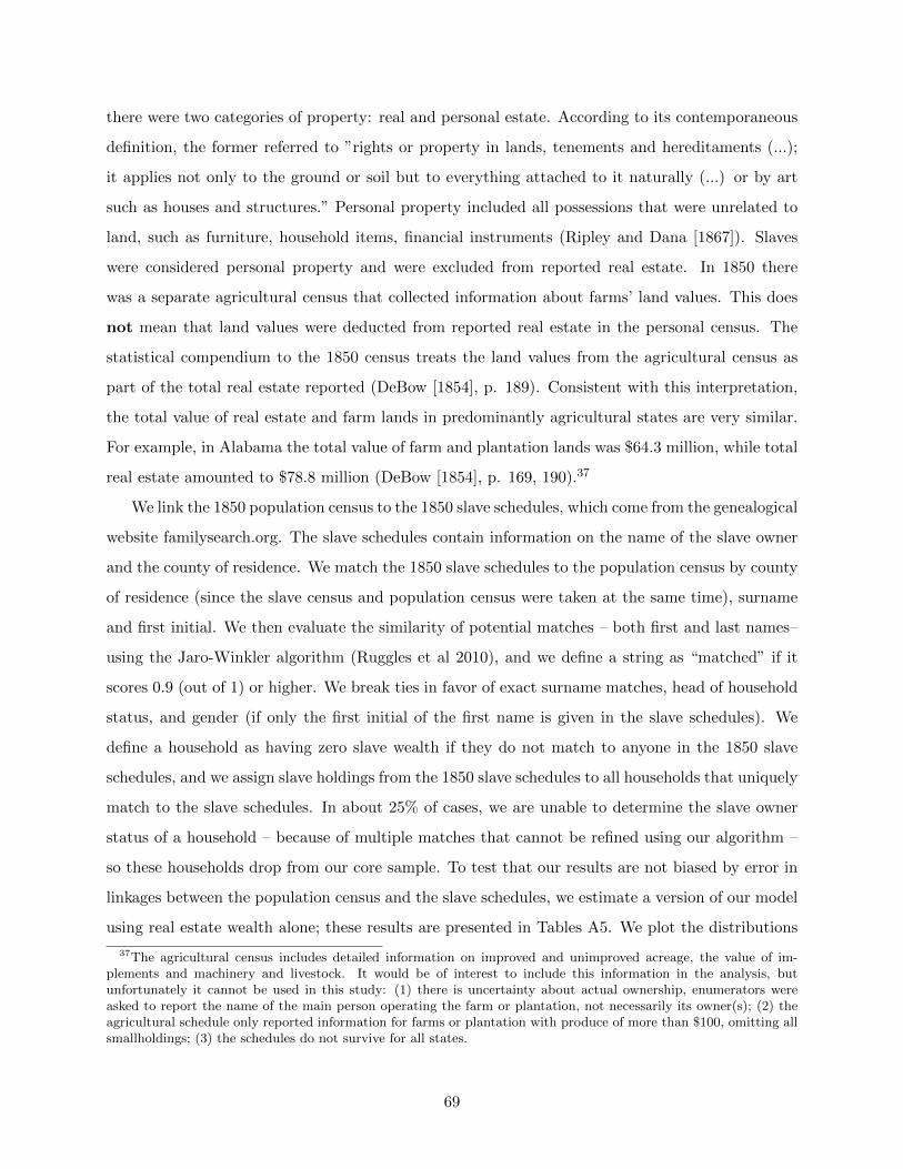
there were two categories of property: real and personal estate. According to its contemporaneous

definition, the former referred to ”rights or property in lands, tenements and hereditaments (...);

it applies not only to the ground or soil but to everything attached to it naturally (...) or by art

such as houses and structures.” Personal property included all possessions that were unrelated to

land, such as furniture, household items, financial instruments (Ripley and Dana [1867]). Slaves

were considered personal property and were excluded from reported real estate. In 1850 there

was a separate agricultural census that collected information about farms’ land values. This does

not mean that land values were deducted from reported real estate in the personal census. The

statistical compendium to the 1850 census treats the land values from the agricultural census as

part of the total real estate reported (DeBow [1854], p. 189). Consistent with this interpretation,

the total value of real estate and farm lands in predominantly agricultural states are very similar.

For example, in Alabama the total value of farm and plantation lands was $64.3 million, while total

real estate amounted to $78.8 million (DeBow [1854], p. 169, 190).37

We link the 1850 population census to the 1850 slave schedules, which come from the genealogical

website familysearch.org. The slave schedules contain information on the name of the slave owner

and the county of residence. We match the 1850 slave schedules to the population census by county

of residence (since the slave census and population census were taken at the same time), surname

and first initial. We then evaluate the similarity of potential matches – both first and last names–

using the Jaro-Winkler algorithm (Ruggles et al 2010), and we define a string as “matched” if it

scores 0.9 (out of 1) or higher. We break ties in favor of exact surname matches, head of household

status, and gender (if only the first initial of the first name is given in the slave schedules). We

define a household as having zero slave wealth if they do not match to anyone in the 1850 slave

schedules, and we assign slave holdings from the 1850 slave schedules to all households that uniquely

match to the slave schedules. In about 25% of cases, we are unable to determine the slave owner

status of a household – because of multiple matches that cannot be refined using our algorithm –

so these households drop from our core sample. To test that our results are not biased by error in

linkages between the population census and the slave schedules, we estimate a version of our model

using real estate wealth alone; these results are presented in Tables A5. We plot the distributions

37The agricultural census includes detailed information on improved and unimproved acreage, the value of im-plements and machinery and livestock. It would be of interest to include this information in the analysis, butunfortunately it cannot be used in this study: (1) there is uncertainty about actual ownership, enumerators wereasked to report the name of the main person operating the farm or plantation, not necessarily its owner(s); (2) theagricultural schedule only reported information for farms or plantation with produce of more than $100, omitting allsmallholdings; (3) the schedules do not survive for all states.

69

of our 1850 household asset measures in Figure A2.

Marriage Records

We obtain a list of marriages contracted in 9 southern states from the genealogical website fam-

ilysearch.org. These records are available for a subset of counties; details about the coverage of

these records are given in Table A4. These records give us information about the bride’s full name,

the groom’s full name, the county of marriage, and the date of marriage. We link these records

to the census of 1850 by groom’s first name, groom’s last name, and bride’s last name. We drop

observations in which only the groom’s or bride’s first initial is provided, as we feel this provides

insufficient information to make quality links.

We first merge our marriage records with the 1850 census by: (1) Groom’s first initial; (2)

Bride’s first initial; (3) NYSIIS code for groom’s surname (Atack and Bateman 1992). Because we

only have information on names with which to narrow our list of potential matches, it is necessary

to impose some filter prior to evaluating the similarity of our matches. We then calculate a measure

of string similarity between names in our marriage records and names in the census using the Jaro-

Winkler algorithm. We define two strings as “matched” if they score 0.8 (out of 1) or higher, or if

only a first initial is recorded in the census and first initials match. We keep unique matches only,

and then we drop matches with only first initials reported in the census. We are aiming for accuracy

at the expense of sample size. This procedure yields numerous multiple matches – see table A2 for

details. So, we narrow down our matches using information on implied ages at marriage, using the

procedure described in the main body of the text. Evidence on the accuracy of our unique matches

can be found in table A3 and figure A1.

1840 Census

We compute a measure of “familial assets” by averaging log slave wealth by state and surname,

and we link this to our matched sample by state of birth and surname (using the maiden name

from marriage records for women). So, the pre-marital wealth of person i with surname j who was

born in state s will be:

wi,j,s =1

Kj,s

Kj,s∑k=1

wk,j,s

Here, Kj,s is the number of households in state s headed by someone with the surname j. We

match the spelling of surnames exactly. We are able to obtain an estimate of pre-marital wealth for

70

76% of our linked sample, among couples in which both the husband and wife are southern born.

One thing to point out is that the distribution of wi,j,s depends on Kj,s, with more common

names having a more compressed distribution than uncommon names. In our linked sample, wi,j,s

among surnames occurring only has a mean of 2.8 and a standard deviation of 3.7; conversely, wi,j,s

among surnames occurring 2-100 times has a mean of 2.8 and a standard deviation of only 1.9.

Among names occurring 100 times or more, wi,j,s has a mean of 2.7 and a standard deviation of

0.75. The median man in the sample has a name occurring 15 times, while the median woman in

the sample has a name occurring 28 times. This difference is due to the fact that we are performing

links using men’s surnames, which biases us against finding men with common surnames.

Given these distributional features of our measure of wealth, it is worth mentioning some of

its properties. Suppose there is no linkage error. So, if we observe person i with surname j from

state s, we assume that this person’s family is one of the Kj,s households used to compute wi,j,s.

Suppose also that there is error in the measurement of “true” log wealth (w∗), so that measured

wealth (w) is given by:

w = w∗ + ε

First, notice that our wealth measure is “unbiased” in the sense that it does not differ systematically

from w∗i :

E[w∗i − wi,j,k] = E[w∗]− E[w∗] = 0

We also derive the expected squared deviation of w∗i from wi,j,k, which captures the variance of

our wealth measure, and is a function of Kj,s and other unknown parameters. Suppose that the

variance of ε is σ2ε , and the variance of w∗ for state s and surname j is σ2

j,s. Further, suppose that

the covariance of w∗i,j,s and w∗k,j,s is ρj,s, for any i, k. Then, it can be shown that:

E[w∗i − wi,j,k]2 =σ2ε

Kj,s+Kj,s − 1

Kj,s(σ2j,s − ρj,s)

After some algebra, this follows from the assumption that ε is IID with mean zero, and that wi,j,s is

one of the Kj,s observations used to compute wi,j,k. Intuitively, this is increasing in the variance of

the measurement error term, increasing in the dispersion of w∗ within surname-state groups, and

decreasing in the covariance of w∗ within surname-state groups.

Given that we have no information about these parameters, it is difficult for us to address this

empirically. However, notice also that the overall variance of measurement error also depends on

71

Kj,s. In particular, as Kj,s increases, measurement error generated by ε becomes less important, but

measurement error generated by dispersion within surname-state groups becomes more important.

This is because, as Kj,s increases, wi,j,s starts to converge to the median w. This tends to cause the

expected squared deviation of w from wi,j,s to start to grow. We can address this by overweighting

observations with less common names. Specifically, we compute the following weight for men from

state s with surname j and women from state t with surname k:

λjs,kt =

(1

Kj,s+(Kj,s − 1

Kj,s

)σ2j,s

)−1/2(1

Kk,t+(Kk,t − 1

Kk,t

)σ2k,t

)−1/2

Here, Kj,s is the number of households in state s with surname j, and σ2j,s is the sample variance of

w among households in state s with surname j. This is an attempt at weighting by the inverse of

the geometric mean of the variance of measurement error associated with the husband’s and wife’s

wealth. These results can be found in Table A5

72

C Additional Tables and Figures

73

Figure A1: Accuracy of Matches

Figure 2: Accuracy matches. This figure evaluates the accuracy of our matches using the implied age atmarriage. The left panels present distributions of the age-at-marriage of husbands and wifes in our matchedsample who got married in 1840 and 1849. The right panels present ages-at-marriage for randomly matchedpersons in the 1850 census, assuming they were either married in 1840 or 1849.

30

Note: This figure evaluates the accuracy of our matches using the implied age at marriage. The left panels presentdistributions of the age-at-marriage of husbands and wifes in our matched sample who got married in 1840 and1849. The right panels present ages-at-marriage for randomly matched persons in the 1850 census, assuming theywere either married in 1840 or 1849.

74

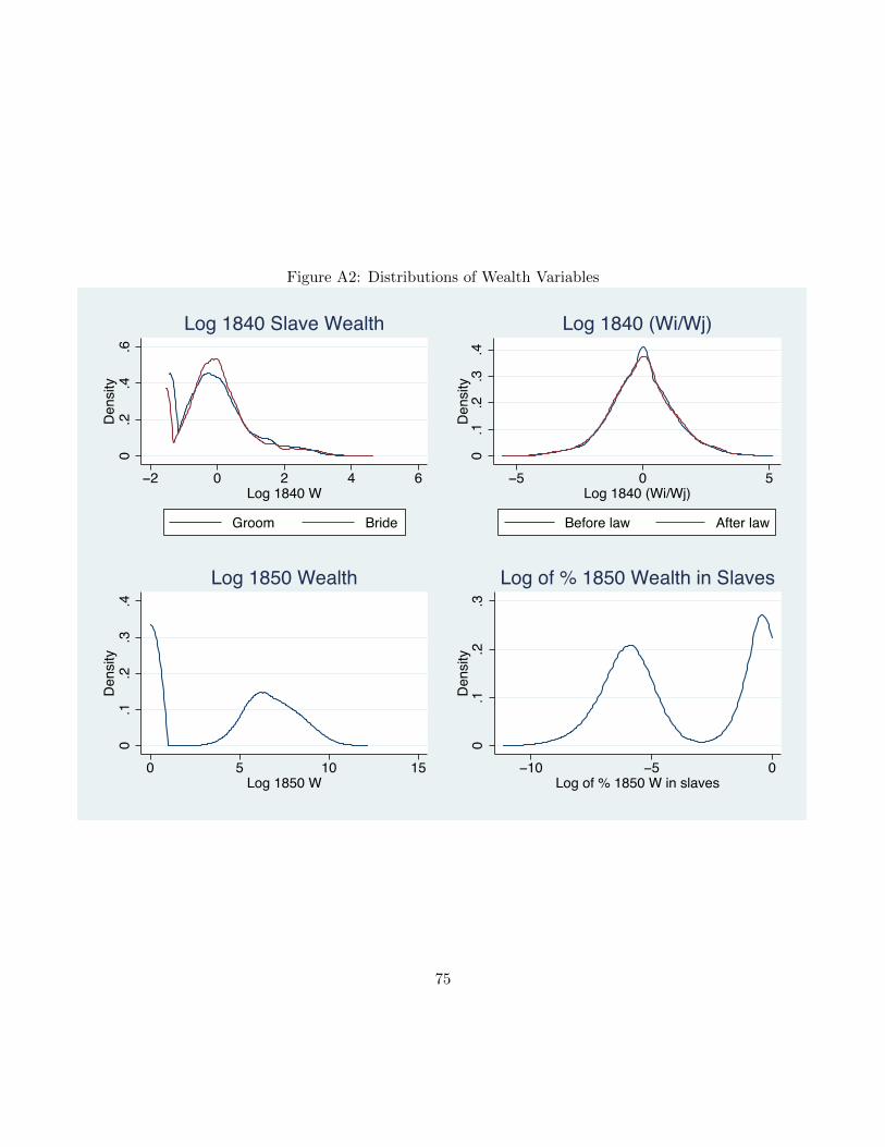
Figure A2: Distributions of Wealth Variables

0.2

.4.6

Den

sity

−2 0 2 4 6Log 1840 W

Groom Bride

Log 1840 Slave Wealth

0.1

.2.3

.4D

ensi

ty−5 0 5

Log 1840 (Wi/Wj)

Before law After law

Log 1840 (Wi/Wj)

0.1

.2.3

.4D

ensi

ty

0 5 10 15Log 1850 W

Log 1850 Wealth

0.1

.2.3

Den

sity

−10 −5 0Log of % 1850 W in slaves

Log of % 1850 Wealth in Slaves

®

75

Figure A3: Kaplan-Meier Survival Estimates – Passage of New Laws

0.00

0.25

0.50

0.75

1.00

Below average Above average

By Cotton Intensity.0

6.0

8.1

.12

.14

Raw

Cot

ton

Pric

e, $

1836 1841 1846 1851 1856Year

®

0.00

0.25

0.50

0.75

1.00

Below average Above average

By Slave Intensity

300

400

500

600

700

Aver

age

Slav

e Pr

ice,

$

1836 1841 1846 1851 1856Year

®

Note: Cotton intensity is defined as the ratio of pounds of cotton picked in 1840 to the white population, atthe state level (Haines & ICPSR 2010). Slave intensity is the ratio of slaves to whites in 1840, at the statelevel ((Haines & ICPSR 2010). Cotton and slave prices are taken from the Historical Statistics of the UnitedStates (Carter et al 2006). Sample includes all southern states (adding Maryland and South Carolina to the basesample). Kaplan-Meier survival estimates represent the probability of not having passed a property law in eachyear, subdivided by cotton and slave intensity.

76

Figure A4: Robustness to Different Wealth Transformations

0.2

.4.6

Coe

ffici

ent

0 10 20 30 40 50# added before taking log

Coeff. on post law X log(Wm/Wf)

Note: Plots OLS estimates of the coefficient on [Husband’s log(W) - Wife’s log(W), 1840] × Post Law fromour baseline specification, when different constants are added to wealth variables before taking logs. Dashed linesrepresent 95% confidence bands (based on standard errors clustered at three levels: state-year of marriage, groom’ssurname-birth state, and bride’s surname-birth state).

77

Figure A5: Placebo Test: Marriage Dates Randomly Assigned

01

23

4Density

0 0.227Coefficient

®

Note: Plots distribution of OLS estimates of the coefficient on [Husband’s log(W) - Wife’s log(W), 1840] × PostLaw from 10,000 iterations of our baseline specification, in which marriage dates are randomly assigned.

78

Table A1: Mortgages East Feliciana ParishName Year Loan ($) Collateral LTV

No. of Slaves Value of land ($) Total Value ($)

Joseph Kirkland 1825 4,900 32 4,646 13,510 0.36(N/A) (N/A)

Frederick Williams 1828 1,800 7 3,630 5,401 0.33(N/A) (N/A)

Margaret Johnson 1845 750 8 0 2,736 0.27(Morris) (10) (9,220)

John Kernan 1845 1,600 7 0 2,394 0.67(6) (5,200)

Henry Lathrop 1845 700 7 0 2,394 0.29(11) (20,000)

Stephen Johnson 1846 1,600 10 0 3,580 0.45(10) (9.220)

Elizabeth Chaney 1846 12,000 28 0 10,024 1.20(Howell) (40) (23,060)

Henry Knox 1846 1,320 2 0 716 1.84(0) (4,550)

John L. DeLee 1848 5,000 51 4,356 25,419 0.20(54) (34,800)

John McKneely 1854 18,500 50 7,260 37,310 0.50(70) (53,000)

Alexander and 1855 18,725 76 7,623 53,223 0.35John Y Mills (81) (26,000)

Benajah D Doughty 1855 1,260 6 0 3,600 0.35(5) (2,950)

George Purnell 1856 11,000 24 6,534 22,278 0.49(56) (39,500)

Daniel McMillan 1856 10,776 20 0 13,120 0.82(19) (13,000)

Bailey D. Chaney 1857 13,000 32 10,309 30,661 0.42(35) (39,000)

Sarah Sims 1857 1,150 5 0 3,180 0.36(0) (12,500)

Average 0.45

This table list 16 mortgages from Kilbourne (1995) for which detailed information is available. The numbers in parentheses indicate the

number of slaves or value of real estate reported in the 1850 census. All mortgages were recorded in East Feliciana Parish in Louisiana.

The year column refers to the year a mortgage was passed. The loan amount is the notional value of the mortgage. The columns under

the heading ”collateral” indicate the assets underlying the mortgage: the number of slaves and a certain acreage of land. Kilbourne lists

land in acres, we present the $ value, using an average price for improved and unimproved land in East Feliciana Parish of $7.26 per

acre. This number comes from the 1850 census. We calculate the total value of the collateral using the average slave price in the year

a mortgage was recorded. This data comes from (Carter et al 2006). The final column with ”LTV” calculates the loan-to-value ratio.

Both slave and land values are approximations. If acreage only referred to improved or unimproved land, values would be different.

Exact slave values depend on sex and age, which we don’t capture in this table. As a result, individual LTVs are approximate only.

79

Table A2: Rates of Matching to 1850 Census by State% at least 1 match % at least 1 full % unique match % matched Total number

to census (incl. first name match to census using age of marriageon first initials) to census information records

Alabama 0.585 0.487 0.176 0.236 23,843Arkansas 0.534 0.445 0.167 0.218 5,846Florida 0.525 0.455 0.162 0.197 2,378Georgia 0.614 0.518 0.196 0.256 27,689Kentucky 0.558 0.476 0.171 0.216 43,584Louisiana 0.288 0.219 0.067 0.086 6,140Mississippi 0.636 0.527 0.210 0.286 10,635North Carolina 0.569 0.496 0.222 0.266 23,050Tennessee 0.308 0.243 0.089 0.120 81,380Texas 0.493 0.378 0.139 0.215 6,502Virginia 0.618 0.562 0.243 0.283 26,813

Total 0.489 0.411 0.158 0.203 257,860

Table A3: Accuracy of Matched DataProb. living in state Prob. husband born in state Prob. wife born in state

Married in All southern Married in All southern Married in All southernstate couples state couples state couples

Alabama 0.726 0.074 0.224 0.022 0.380 0.034Arkansas 0.795 0.029 0.116 0.002 0.181 0.004Florida 0.801 0.008 0.096 0.001 0.225 0.002Georgia 0.800 0.091 0.572 0.078 0.681 0.088Kentucky 0.865 0.137 0.637 0.090 0.731 0.101Louisiana 0.794 0.044 0.515 0.015 0.583 0.019Mississippi 0.770 0.052 0.203 0.009 0.310 0.014North Carolina 0.831 0.098 0.806 0.169 0.831 0.152Tennessee 0.781 0.132 0.554 0.102 0.646 0.117Texas 0.820 0.028 0.030 0.001 0.074 0.002Virginia 0.890 0.160 0.833 0.194 0.861 0.180

80

Table A4: Coverage of 1840 Marriage Record Data% counties with % Population living in

State # Marriage records marriage record data counties with marriagerecord data

Alabama 27,934 0.67 0.75Arkansas 7,186 0.49 0.56Georgia 32,756 0.74 0.78Kentucky 50,507 0.64 0.71Louisiana 5,277 0.19 0.37Mississippi 12,838 0.47 0.65North Carolina 27,564 0.73 0.76Tennessee 95,371 0.65 0.72Virginia 31,292 0.48 0.54

81

Table A5: Effect of Married Women’s Property Laws on 1850 Gross Investment - Additional Robustness 1(1) (2) (3) (4)

Dep. var. log(Gross investment), 1850

Post Law -0.126 -0.138 -0.009 -0.141(0.110) (0.093) (0.127) (0.188)

[Husband’s log(W) - Wife’s 0.134 0.162 0.218 0.178log(W), 1840] × Post Law (0.070)* (0.068)** (0.072)*** (0.108)

Adj-R2 0.157 0.190 0.190 0.197Obs 27090 24933 24933 27090

Age at marriage FE Y Y Y YBirthstate and literacy FE Y Y Y YFrequency names, bin FE Y Y Y YState specific lin. time trend Y Y Y Y

OLS estimates. All regressions contain state and year of marriage fixed effects, husband’s and wife’s 1840 logwealth, and interactions between premarital wealth variables and state and year of marriage fixed effects. Grossinvestment : value of household’s real estate and slave holdings in 1850 census, gross of debt. When estimatingOLS the dependent variable is log(1+ Gross investment). Husband’s/Wife’s 1840 wealth: average log slave wealth(log(# slaves ×377 + 1)) of individuals with the same surname as the husband and wife in their respective statesof births in the 1840 census. State exemption level : $ amount exempt in case of insolvency. Frequency names,bin FE : we calculate the relative prevalence of husband’s and wife’s family names per state. We summarizethis information in 10 bins, where bin 1 includes the rarest family names, and bin 10 the most common ones.All (continuous) independent variables are normalized by their standard deviation; reported coefficients thereforeindicate by what % gross investment changes in response to a one standard deviation increase in the right handside variable. All interactions with the 1840 wealth variables are in deviations from the mean. The coefficient onPost Law therefore measures the effect of the passage of a Married Woman Property Act on a household with anaverage wealth difference. Column (1) defines gross investment as real estate assets only, relaxing the constraintthe observations be linkable to the 1850 slave schedules. Column (2) relaxes the constraint that couples be residentin their state of marriage in 1850, and adds state of residence fixed effects. Column (3) also includes couples whoare married in a state other than their state of residence, but defines protection status based on state of residencenot marriage. Column (4) weights the regression by λjs,kt, as defined in Appendix B. We use real estate as thedependent variable, as linking from the population to the slave census imparts additional error (correlated withthe commonness of surnames) which this weight is not necessarily appropriate for. Standard errors (clustered atthree levels: state × year-of-marriage, groom’s surname-birth state, bride’s surname-birth state) are reported inparentheses: * p < 0.10, ** p < 0.05, *** p < 0.01.

82

Table A6: Effect of Married Women’s Property Laws on 1850 Gross Investment - Additional Robustness 2(1) (2) (3) (4) (5) (6)

Dep. var. log(Gross investment), 1850

Post Law 0.568 0.271 0.340 -0.185 -0.199 -0.197(0.378) (0.389) (0.414) (0.096)* (0.101)** (0.117)*

[Husband’s log(W) - Wife’s 0.238 0.233 0.232 0.237 0.185 0.185log(W), 1840] × Post Law (0.082)*** (0.079)*** (0.080)*** (0.087)*** (0.084)** (0.085)**

Adj-R2 0.112 0.211 0.212 0.089 0.203 0.203Obs 19672 19672 19672 12854 12854 12854

Age at marriage FE N Y Y N Y YBirthstate and literacy FE N Y Y N Y YFrequency names, bin FE Y Y Y N Y YState specific lin. time trend N N Y N N Y

OLS estimates. All regressions contain state and year of marriage fixed effects, husband’s and wife’s 1840 logwealth, and interactions between premarital wealth variables and state and year of marriage fixed effects. Grossinvestment : value of household’s real estate and slave holdings in 1850 census, gross of debt. When estimatingOLS the dependent variable is log(1+ Gross investment). Husband’s/Wife’s 1840 wealth: average log slave wealth(log(# slaves ×377 + 1)) of individuals with the same surname as the husband and wife in their respective statesof births in the 1840 census. State exemption level : $ amount exempt in case of insolvency. Frequency names,bin FE : we calculate the relative prevalence of husband’s and wife’s family names per state. We summarizethis information in 10 bins, where bin 1 includes the rarest family names, and bin 10 the most common ones.All (continuous) independent variables are normalized by their standard deviation; reported coefficients thereforeindicate by what % gross investment changes in response to a one standard deviation increase in the right handside variable. All interactions with the 1840 wealth variables are in deviations from the mean. The coefficient onPost Law therefore measures the effect of the passage of a Married Woman Property Act on a household with anaverage wealth difference. Columns (1)-(3) include interactions between name frequency bins and marriage stateand year fixed effects. Columns (4)-(6) drop states that never pass a property law. Standard errors (clustered atthree levels: state × year-of-marriage, groom’s surname-birth state, bride’s surname-birth state) are reported inparentheses: * p < 0.10, ** p < 0.05, *** p < 0.01.

83