1  

Banking Network and Systemic Risk via Forward‐Looking Partial Default Correlations 

 Jorge A. Chan‐Lau*, Chienmin Chuang†, Jin‐Chuan Duan‡, and Wei Sun§ 

(May 3, 2016)     

Abstract  

This paper studies systemic risk  in a global network with over 1,000 exchange‐traded banks. Network construction follows a methodology comprising  three parts:  (1)  the use of  the default correlation model of Duan and Miao (2015) to produce a forward‐looking probability of default  (PD)  total  correlation matrix  and  then  transform  it  into  a partial  correlation matrix  by  applying  the  CONCORD  algorithm;  (2)  the  measurement  of  banks’  systemic  importance  hinging  on  six network centrality indicators based on the partial correlations, which represent  the direct  connections  among banks;  and  (3)  a  graphical analysis of the global banking network which can then be partitioned into  overlapping  bank/group  centric  local  communities.  We  then specifically study  the banks’ systemic  importance  in 2008 and 2014. Using  the  2014  sample,  we  are  able  to  compare  the  systemic importance  rankings  under  alternative  measures,  including  G‐SIBs identified  by  the  Financial  Stability  Board.  Our  results  suggest  the Board rankings appear biased  towards singling out  large  institutions as systemic, with connectivity playing a rather minor role.    Keywords:  systemic  risk,  banking  network,  forward‐looking, probability of default, partial correlation, banking community  JEL Code: G17, G21, G28 

    

                                                            * Chan‐Lau is with the International Monetary Fund. The views expressed in this document are those of the author and do not necessarily represent those of the IMF or IMF policy. Email: jchanlau@imf.org † Chuang is with Risk Management Institute, National University of Singapore. E‐mail: rmicc@nus.edu.sg ‡ Duan is with Department of Finance, Risk Management Institute, and Department of Economics in the National University of Singapore. E‐mail: bizdjc@nus.edu.sg § Sun is with Risk Management Institute, National University of Singapore. E‐mail: rmisw@nus.edu.sg 

2  

1. Introduction  The  recurrence  of  financial  crises  entails  large  costs  directly  associated  with  disruptions  in  the banking  system  and  huge  impacts  indirectly  on  the  real  economy,  as  evidenced  by  the  global financial  crisis of 2008 and onward. That  financial  crisis has naturally  focused both academic and policy work on  the  identification of  systemic  risk  in  the  financial  system, and  in particular,  in  the global banking network.  To  this  end,  a  variety  of  systemic  risk measures  emphasizing  connectedness  between  banks  and other financial firms have been proposed. Examples include the equity returns volatility (Demirer et al.,  2015),  capital  shortfall  of  an  individual  institution  in  the  crisis  (Acharya  et  al.,  2012),  CoVar (Adrian and Brunnermeier, 2014), and  insurance premium against a firm’s financial distress (Huang et al., 2009). The construction of these measures relies more or  less on equity returns, which only imply  the risk  indirectly.  In addition,  these measures are backward‐looking  in nature and  thus can only be of  limited use when  it comes  to predicting  the  future.  In  this paper, we contribute  to  the literature by creating a directly  relevant and  forward‐looking measure of  risk —  the probability of default (PD). PD captures a firm’s likelihood of not fulfilling its financial obligations over some future horizon.  It  focuses  directly  on  the  realization  of  a  rare  event  of  significance, which may  trigger cascading defaults and cause widespread distress throughout the financial system.   Measuring  the  connectedness  between  banks  is  a  crucial  step  in  constructing  a  proper  financial network. Connectedness is, not surprisingly, one among several criteria that the Basel Committee on Banking Supervision considers  in assessing the global systemic  importance of a bank (BCBS, 2013). Connectedness  between  financial  jurisdictions  has  also  played  a  role  in  determining  whether countries should undergo a mandatory financial sector assessment by the  IMF on a recurring basis (Demekas et al., 2013).   Correlation, which captures the tendency of two parties moving together, or their linear dependence, has been commonly used to serve this purpose (e.g. Tumminello et al., 2010). Although intuitive, the correlation  contains  both  direct  and  indirect  impacts  from  the  rest  of  the  system.  It  naturally confounds the measurement of the direct connection between the two parties, which we believe a good network ought to reflect. To disentangle the direct connection between banks in terms of their future  default  likelihoods,  we  contend  that  partial  correlations  are  more  appropriate,  a  view advanced first by Kennett et al. (2010).  Most of  the work on  financial networks, which we will  review  in more detail  in  the next  section, relies on  the historical, past  co‐movements and/or  correlations of  stock  returns or other market‐based  risk measures.  In  contrast, we  choose  to  construct  a  dynamic,  ever‐evolving  and  forward‐looking default correlation network. We choose not to use historical correlations of PDs, despite the fact that they are easy to calculate from the time series of PDs available from databases managed by the Credit Research Initiative (CRI) at the Risk Management Institute (RMI) of the National University of Singapore, Moody’s Analytics, Kamakura, or Bloomberg. Historical correlations would  represent the connectedness between banks  for a  fixed horizon, say, one month, averaged over a  long  time span. This averaged measure of co‐movement is unlikely to adequately reflect connectedness going forward. Much  like  forward‐looking volatilities which are  informative beyond  the sample standard deviation computable  from  the past data, correlations among PDs are expected  to be dynamic  in response to the state of economy.   Instead, we use the default correlation model of Duan and Miao (2015) to generate a set of forward‐looking PDs for a specific horizon of interest, which reflects the current market conditions while also capturing the eventuality that some firms may cease to be publicly traded or disappear for reasons other  than default. Our  forward‐looking PDs are  constructed  for over 1,000 banks  in  the RMI‐CRI 

3  

database and we use them to obtain the regularized partial correlation matrix, which allows isolating the direct dependence between  two  firms. This matrix  serves as  the basis  for building our global banking network.  Regularization  is  required  for  two  reasons. The  first  reason  is  technical, as  the estimation of high dimensional partial correlation matrices can be unstable in the absence of regularization. The second reason has an economic underpinning: without regularization, the partial correlation matrix would be relatively dense, which would tend to bunch all in one big global component, with all banks being systemically  important. By  imposing a regularization condition, a substantial number of edges may drop from the network but we ensure that there are no totally disconnected banks,  i.e. “orphans.” This  “regularized”  network,  therefore,  is  consistent  with  the  intuition  of  a  globally  connected banking system with only a certain number of systemic firms.  Besides the use of  forward‐looking PDs, another novel  feature of our analysis  is that edges, which capture the strength of the connection between banks, are not only weighted by the values of the partial  correlations  but  also  by  firm  characteristics,  i.e.  their  share  in  the  network’s  total  assets. While node characteristics have been used before  in Demekas et al.  (2013),  the resulting network was reduced to an unweighted network after the removal of edges with low weights. In contrast, we calculate several centrality measures using the weighted network, and the analysis of the measures help us determining the systemic ranking of banks.  For  comparison  purposes, we  also  construct  partial  correlation  networks with  historical  PDs  and stock returns, respectively, for the same sample of banks. There are substantial differences between the  systemic  risk  rankings  obtained  from  historical,  backward‐looking  correlations  and  those obtained using the forward‐looking partial correlations. These differences persist whether the edges are weighted or not by the size of the firms, suggesting that our approach based on forward‐looking correlations  is  materially  different.  More  importantly,  the  overlap  between  the  set  of  global systemically  important  banks  determined  by  the  Financial  Stability  Board  (FSB)  and  the  forward‐looking PD  systemic  risk  ranking  is  substantial only when  edges  are weighted by  size. We  argue, hence,  that  the  FSB  ranking  is  severely  biased  towards  singling  out  large  institutions,  and connectivity plays a rather minor role.  Before offering a detailed explanation of the methodology and a discussion of the results, the review of the related literature next serves to frame and put into context the contribution of this paper.   

2. Related Literature  A recent strand of  the  literature has  focused on  the dimensions of systemic risk and related costs associated with the possibility of multiple failures among banks. For  instance, Acharya et al. (2012) measure the cost of a financial crisis by assessing potential capital shortfalls driven by  large equity price declines relative to required regulatory capital ratios. While it is not necessarily the case, large capital shortfalls are  likely  to occur simultaneously since  there  is dependence between  the equity price movements of individual firms and the overall market (Brownlees and Engle, 2015). Duan and Zhang (2013) use asset‐liability dynamics with several common risk factors to measure the systemic exposure and systemic  fragility arising  from cascading defaults, which correspond  to  the expected losses and pervasiveness of defaults under a stress scenario similar to that  in Brownlees and Engle (2015).  Rather than relying on dependence through common risk factors, other measures  look at pairwise dependence  on  the  movement  of  equity  prices  in  distress  periods,  i.e.  CoVaR  (Adrian  and 

4  

Brunnermeier, 2014), or risk measures such as credit default swap  (CDS) spreads,  i.e. CoRisk  (IMF, 2009;  Chan‐Lau,  2013,  Chapter  6).  In  these  approaches,  quantile  regressions  can  capture  the dependence between  two  firms after  correcting  for  the effect of common drivers of  risk,  such as cyclical indicators or volatility indices. Results by Patro et al. (2013) show that simple risk indicators based on daily stock return pair‐wise correlations seem to capture well changes  in systemic risk  in the U.S. financial system.  While pairwise dependence measures can serve to construct a financial network by connecting two banks  with  an  edge  weighted  by  the  dependence  measure,  the  edges  may  still  be  capturing dependence effects from a source independent from the two banks, i.e., common dependence with a  third  bank  or  a  set  of  other  banks.  From  a  network  perspective,  hence,  it may  be  better  to construct the network following a global rather than a pairwise approach. Furthermore, the pairwise approach could be subject to some estimation issues. For instance, a correlation matrix constructed using  pairwise  correlations  based  on  time  series  observations  of  unequal  length may  not  yield  a legitimate correlation matrix.   Mantegna (1999)  is an earlier example of a global approach for constructing financial networks.  In this network, nodes (i.e., firms) are connected by edges weighted by the correlation of their equity returns. Tumminello et al. (2010) expand on this work, by constructing hierarchical trees, correlation based trees and networks from stock return correlation matrices.   In  a  similar  vein, Billio  et  al.  (2012) use monthly  stock  returns  for  financial  institutions,  including hedge funds, broker/dealers, banks, and  insurers, to construct a Granger causality network, where edges  between  firms  run  in  the  direction  of  non‐linear Granger  causality. Billio  et  al.  (2013)  use credit  spreads‐based Granger  causality networks  to analyze  interconnectedness between  financial firms and sovereign countries. Since there are common drivers of equity returns as suggested by the empirical  evidence  from  factor pricing models  (Ferson, 2003,  among others),  as well  as of  credit spreads, measures  based  on  plain  correlations  or  Granger  causality may  be misleading when  it comes to quantifying dependence between firms.1  To  a  certain  extent, using  stock  return  residuals  after  correcting  for  common  factors or principal components could remove the effects of other firms on the dependence between two firms. But the choice  of  common  factors  or  number  of  principal  components  is  non‐trivial.  Spatial‐dependence methods,  developed  in  the  panel  vector  autoregression  literature,  could  be  applied  to  remove strong common factors.2 Craig and Saldias (2016), building on work by Bailey et al.  (2015b), follow this  approach  to  construct  a  banking  network  using  stock  returns,  approximating  the  common factors with principal components.  Another alternative is to use partial correlation analysis, as in the analysis of stock returns networks by Kennett et al. (2010). Their results highlight substantial differences between standard correlation networks and  the  corresponding partial  correlation ones. More  recently, Barigozzi and Brownlees (2016)  also  use  partial  correlations  to  construct  financial  networks,  building  on  the  vector autoregressive model introduced by Diebold and Yilmaz (2014).   Moving  beyond  stock  return  correlations,  Demirer  et  al.  (2015)  propose  that  a  directed  edge corresponds  to  a  firm’s  stock  returns’  contribution  to  the  generalized  forecast  error  variance decomposition of the other firm’s stock returns, where the decomposition is obtained as suggested by Koop et al. (1996), and Pesaran and Shin (1998). Results by Lanne and Nyberg (2016), however, suggest that these measures may not be comparable across time since,  in contrast to the forecast 

                                                            1 See Chudik et al. (2011) and Bailey et al. (2015a). 2 See the survey by Canova and Ciccarelli (2013). 

5  

variance decomposition  in a structural vector autoregressive model, the sum of the proportions of the impact accounted for the innovations may not sum to unity.   A common  feature  shared by  the different approaches presented  in  this  section  is  that  the price‐based measures used, either based on stock returns or credit spreads, are backward‐looking  in the sense  that  they  only  capture  co‐movements  of  past,  observed  data.  As  highlighted  in  the introduction, they may fail to capture dynamics associated with an evolving economic environment. The  next  section  explains  how  to  construct  forward‐looking  PDs,  allowing  us  to  overcome  the backward‐looking problem faced by earlier studies. 

 3. Methodology   Our approach comprises  three parts:  (1) constructing a  forward‐looking probability of default  (PD) partial correlation matrix for banks under consideration, (2) utilizing the partial correlation matrix to devise measures for ranking banks in terms of their systemic importance, and (3) building a banking community centered at a bank or a group of banks so  that different communities of  interest may naturally overlap.   For the first part, we adopt the default correlation model of Duan and Miao (2015) to produce via simulation a forward‐looking PD total correlation matrix for any future horizon of interest in a time‐consistent manner.  The  total  correlation matrix  is  then  used  to  obtain  the  corresponding  partial correlation matrix by applying the CONCORD  (CONvex CORrelation selection methoD) algorithm of Khare,  et  al.  (2015).  We  choose  to  rely  on  partial  PD  correlations,  because  they  are  ideal  for disentangling the pure and direct default risk  linkages between two banks as opposed to reflecting the indirect influence via third parties.   With the forward‐looking PD partial correlation matrix in place, we then focus on the two remaining components of our methodology. To measure systemic importance of a bank in the network, we rely on the concept of network centrality where the nodes and edges are defined by the forward‐looking PD partial  correlation matrix.  Six measures of network  centrality are used, and of which  four are standard  and based on network  edge  characteristics,  and  two  are novel.  The  two new  centrality measures  introduced here utilize  the eigenvector centrality concept by explicitly  incorporating  the size of banks,  i.e., combining edge and node characteristics.3 For example, a  large bank, say, HSBC, may be  connected with many  smaller banks. A  simple  size‐weighted measure would make  these connections  less  important. The edge‐node combined eigenvalue centrality would, however, make those connected smaller banks systemically more important due to their connection to HSBC, which in turn also increases the systemic relevance of HSBC via feedback.   The  last  component  of  our methodology  is  to  devise  a  bank/group‐centric  banking  community. Instead  of  partitioning  banks  into  non‐overlapping  communities,  a  group‐centric  community  is defined. Within the defining group, a member bank may not have any partial correlation with others, but  it  is nevertheless a member of the community by definition. This group‐centric community can be straightforwardly obtained, be it a global banking community which contains all banks, or, say, a New  York‐centered  banking  community  where  all  New  York‐based  banks  are  included,  with  or 

                                                            3 Demekas et al. (2013), in their financial jurisdictions network, weigh edges using node characteristics such as the PPP‐GDP of  the  jurisdiction and  the  share  in  the global derivatives market of  the banks headquartered there. The weights in their analysis are used to prune edges with values below a certain threshold instead of fundamentally altering systemic importance as in ours. These authors also use the clique percolation method (Palla et al. 2005) for identifying communities which, in contrast to the group‐centric community proposed by us, requires that at least a subset of the banks in the community are fully connected to each other. 

6  

without connections with each other, along with other banks whose partial correlations with at least one New York‐based bank are non‐zero. The  focal group  can also be narrowed down  to  just one bank;  for  example,  forming  a  Banco  Santander‐centered  banking  community. Naturally,  different overlapping communities will emerge to reflect different focal groups.  2.1 Constructing the forward‐looking PD partial correlation matrix  The default correlation model of Duan and Miao (2015)  is adopted to generate forward‐looking PD total correlation matrix, which  is  then used  to deduce  its corresponding partial correlation matrix. The Duan and Miao (2015) model specifies a factor model for one‐month PD and probability of other exits (POE) of individual firms in the universe of exchange‐traded corporates, with the factors being  some  predetermined  credit  risk  indices  constructed  from  the  same  universe  of  corporates.  As reported  in Duan et al. (2012), POEs are many times  larger than PDs for typical US firms. Thus, the survival probability of a firm is largely determined by POE rather than PD. Naturally, POE is critical to default modeling, because the survival probability  is a key determinant of any multiple‐month PD. The Duan and Miao  (2015) model also handles missing data, which naturally occur as a  result of defaults and other corporate exits.   Duan and Miao (2015) employ 11 pairs of predetermined factors consisting of (1) the pair of global median PD and POE based on a pool of over 40,000 exchange‐traded corporates that have PDs and POEs for at least 60 months over the sample period, and (2) 10 pairs of industry median PD and POE based on the Bloomberg Industry Classification System. The PDs and POEs of these firms are taken from  the  Credit  Research  Initiative  (CRI)  database,  a  public‐good  undertaking  at  the  Risk Management  Institute  (RMI) of  the National University of Singapore  (NUS). The RMI‐CRI produces and publishes daily updated  term  structures of PDs, using  the  forward‐intensity corporate default prediction model  of Duan  et  al.  (2012),  for  exchange‐traded  corporates  around  the world. As  of December  2015, RMI‐CRI  provides  PDs, with  horizons  ranging  from  1 month  to  5  years,  on  over 60,000 firms in 119 economies. Among them, over 30,000 corporates are currently active with daily updated PD and POE values. The PD and POE time series in some cases date back to 1990. We use this RMI‐CRI database for the analyses in this paper.  The  factors  (pairwise with one  for PD  and  the other  for POE)  are dynamically  evolving, modeled using a vector autoregressive structure which allows  factor model  residuals  to be also  individually autoregressive.  Since  the  individual  time  series  model  residuals  are  allowed  to  form  locally correlated  clusters,  default  correlations  in  the Duan  and Miao  (2015) model  could  arise  globally and/or locally. The factor model is estimated with a SCAD penalized likelihood method of Fan (1997) to  deal  with  noisy  parameter  estimates  due  to  many  regressors,  or  alternatively  too  few observations.  This  factor model with  sparsely  correlated  residuals  enables  us  to  generate  PDs  during  a  target horizon, say, one year, at any future time point, say, one month later, for any subset of firms in the RMI‐CRI  universe.  The  one‐year  PD  for  a  firm  one  month  later  is  a  random  variable,  and  can therefore be correlated with the one‐year PD of another firm at that time, which  is the kind of PD correlations that we  intend to capture. Operationally, one can simulate forward one month the 11 pairs of  factors along with  individual PD and POE  residuals of  a  target group of  firms. This  initial simulation yields the starting point for a second set of simulations. Moving forward one month, one can further simulate M paths over 12 months for the risk factors and individual PD and POE residuals, and  for each of  the M paths deduce  the  corresponding one‐year PD using  the  standard  survival‐default formula, and finally average over the M paths to compute the Monte Carlo estimate of the one‐year  PD  one month  later. We  repeat  the  procedure  for  every  firm  in  the  target  group  to generate one set of random one‐year PDs one month later.  

7  

 Repeat the two‐step simulation process N times to generate N sets of one‐year PDs for the target group of firms. One is then in a position to estimate the correlation matrix using these N sets of one‐year PDs over the one‐month horizon. In the implementation later, we set M=1000 and N=1000. By increasing M and N, the correlation matrix can be obtained with any desired  level of accuracy, but the sampling error intrinsic to the estimated Duan and Miao (2015) default correlation model cannot be eliminated by increasing simulation accuracy. Note that this correlation matrix is actually for the change in, say, one‐year PDs over, say, one month, because N one‐year PDs for a firm all start from the same one‐year PD one month earlier.   Our next task is to convert the forward‐looking PD total correlation matrix into a partial correlation matrix.  By  definition,  partial  correlation  is  the  residual  correlation  after  subtracting  any  indirect impact from other parties in the system. Empirically, it can be obtained from linear regressions. The problem with this approach  is that the resulting partial correlation matrix will  likely be dense with many  entries  close  to  zero.  These minuscule  entries  tend  to  disguise  the more meaningful  and important relationships that we are after.   To make the partial correlation matrix more sparse and meaningful, a Lasso‐type penalty is typically utilized to trim the partial correlation matrix, which in essence  imposes zero partial correlations on pairs that have weak ties. We apply the CONCORD algorithm  introduced  in Khare et al. (2015) and Oh  et  al.  (2014), which  uses  a  proximal  gradient method  to  solve  an  objective  function with  a purposely  designed  penalty  matrix.  The  CONCORD  algorithm  guarantees  convergence  since  it preserves convexity  through an appropriate selection of weights and  the design of a penalty  term based on the  inverse of the correlation matrix rather than on the partial correlation matrix. This  is not  the case with other penalty‐based methods  for generating sparse partial correlations, such as the SPACE (Sparse PArtial Correlation Estimation) method of Peng et al. (2009).  Following equation (4) of Oh et al. (2014), we set equation (1) as our minimization target with the CONCORD objective function as:   

lndet tr ∥ ∥ (1)  where det ⦁ andtr ⦁  denote the determinant and trace operators, respectively;   is the sample correlation matrix  computed with  a  sample  size  of N;  and where  the  inverse  of  the  correlation matrix,  ,  can be  split as  , where   and  , denote  respectively  the diagonal and 

off‐diagonal elements of  . The  ‐penalty  term  is  ∥ ∥ ∑ | |, where     is  the off‐

diagonal element in   and the scaling parameter  0  determines the shrinkage rate, or how 

aggressively one penalizes the non‐zero entries in  . Cross‐validation by dividing the data sample into randomized training and validating datasets is the usual way to determine the optimal shrinkage rate. However, we choose to select   such that it is just slightly below the value at which an orphan bank, i.e., totally isolated bank in the network, begins to emerge.4  Economic intuition justifies using this selection criterion because in reality, all banks in the banking system should be connected with some other banks.   

                                                            4 We set the tolerance error for finding the optimal   at 10  and the partial correlation precision at 10 . These tolerance and precision levels are set to conserve computing time. The results are not sensitive to further tightening of their levels. 

8  

After obtaining the optimal  , one can compute the partial correlation matrix    whose (i,j) element 

equals   . For the discussion of centrality measures next, let us set   equal to   except that 

its diagonal elements are set to 0 since there is no interest in analyzing the effects of a bank on itself.  2.2 Ranking systemically important banks via different network centrality measures   A  natural  outcome  of  studying  the  linkages  in  a  financial  network  is  to  determine  the  relative importance  of  each  bank, which  could  help  policy makers  rationalize  different  risk management measures/actions.  The  linkages  in  our  analysis  are  described  by  the  forward‐looking  PD  partial correlation matrix. A bank’s systemic importance is its centrality in the network. Different centrality measures  typically  reflect  different  kinds  of  systemic  importance,  and  no  single measure  can  be expected  to serve all purposes well. Here, we utilize  four standard centrality measures hinging on the  concept  of  adjacency  matrix:  degree  centrality,  connection‐strength  centrality,  eigenvector centrality, and connection‐strength eigenvector centrality. For a network with n firms, we define the adjacency matrix A as the n x n matrix whose elements are set to 0 or 1 depending on whether their corresponding elements in   equal 0 or not.   The degree centrality of Bank i is defined as the i‐th row sum of A, whereas the connection‐strength centrality is the i‐th row sum of | |, the absolute value of  , divided by the total number of banks in  the  network.  The  later  normalization  makes  possible  comparing  results  across  networks comprising different number of banks. The eigenvector centrality  is based on the eigenvector of A that corresponds to the  largest eigenvalue. Since A  is a non‐negative matrix, the Perron‐Frobenius theorem implies that this eigenvector can be made to have all non‐negative elements, with the i‐th element representing the centrality of the  i‐th bank. Similarly, the connection‐strength eigenvector centrality  is  the  eigenvector  associated with | |.  The  eigenvector  centrality measures  a  node’s importance by factoring in the extent to which its connected nodes are further connected. In short, it measures  impacts  in a network globally, and has been widely applied to rank the  importance of individual nodes in networks.  The four centrality measures discussed thus far are all based on the number and values of edges to and  from  a node  as opposed  to  the node’s  characteristics beyond  connections,  for  example,  the relative  size  of  a  bank. Moreover,  node’s  characteristics may  also  affect  the  node’s  number  and nature of its connections. For instance, a large, well‐capitalized bank may be better able to provide interbank loans to a large number of counterparties. We thus devise two novel edge‐node combined centrality measures. First,  let   be the size of a bank (total assets measured  in USD) over the total size  (total assets) of  the banking network, and Q be a diagonal matrix with   as  its  i‐th diagonal element. The two new measures are, respectively, the non‐negative eigenvector (corresponding to the  largest  eigenvalue)  of  the  size‐adjusted  adjacency matrix, QAQ  and  that  of  the  size‐adjusted partial  correlation  matrix,  | | .  Under  these  new  centrality  measures,  a  smaller  bank  by connecting  to  a  large  bank will  become  relatively more  important, which  in  turn  feeds  back  to increase the  large bank’s systemic  importance through the eigenvector solution. We favor the two new  centrality  measures  because  they  go  beyond  the  complexity  of  linkages  (i.e.,  edge characteristics).  Since  there  is  little  question  about  bank  size  (i.e.,  a  node  characteristic  beyond connections)  being  critical  to  systemic  importance,  the  two  new  centrality measures  seem more suitable for banking networks.  2.3 Determining the bank/group‐centric banking community  Communities within a network can be constructed as either overlapping or non‐overlapping ones, using quite different  techniques. To create non‐overlapping communities  is  to partition  the nodes into several disjoint sets with methods such as spectral bisection (Fiedler, 1973, and Pothen et al., 

9  

1990), benefit function optimization (Kernighan and Lin, 1970), hierarchical clustering (Scott, 2000), and edge removal (Girvan and Newman, 2002). For our purposes, however, hard partitioning banks into non‐overlapping  communities  is not appealing, because  forcing a bank  to  just belong  to one community is inconsistent with the common notion of banking communities.   An alternative  is  to  create overlapping  communities,  for which  several methods are available;  for example, clique percolation of Palla et al. (2005) and its variants.5 The clique percolation method to create  overlapping  communities  relies  on  first  forming  cliques  based  on  edges  and  then  putting connected cliques into a community. Thus, it is also not ideal for our purpose; for example, a banking community  centered  in  the New York area and  connected by  credit  risk  linkages  should naturally include all New York‐centered banks along with some banks belonging to, say, the London‐centered community.  In short, focal groups (i.e.,  individual banks, financial centers, and countries) are more natural  communities  from  a  user’s  perspective,  and  different  banking  communities  centered  at different focal groups should be allowed to overlap.  We  use  the  network  analysis  tool,  Gephie,  to  graphically  present  banking  communities.  In  the network, each node represents a bank, and the node size is determined by its total asset. Each edge linking two nodes represents a non‐zero partial correlation between the two banks’ forward‐looking PDs. The thickness of the edge represents the connection strength, and the color of the edge reveals a positive (red) or negative (blue) connection. We use the software’s built‐in algorithm ForceAtlas2 to set  the graphical configuration. ForceAtlas2  is a  force‐directed algorithm. Under  this algorithm, the  attraction  and  repulsion  forces  between  the  nodes move  them  around  and  eventually  to  a balanced  state.  Essentially,  this  algorithm  turns proximities  in  a network  into  visual  communities with denser connections  (Jacomy et al. 2014). As per our partial correlation construction method, there will  not  be  any  genuine  orphan  or  unconnected  bank  in  the  overall  banking  network,  but within some communities, certain banks may be orphan banks.   

3.  Global  Banking  Network,  Systemically  Important  Banks,  Banking Communities, and the 2008 Banking Crisis 

 This section illustrates the use of our methodology for assessing the systemic importance of banks. First, the section evaluates how the six different network centrality measures compare to each other; second,  it analyzes their performance vis‐a‐vis the ranking methodology proposed by the Financial Stability Board (FSB), which currently supports the regulatory reform proposals for systemic banks; and third, it assesses their performance during August 2008, in the eve of the global financial crisis.   The sample  includes  firms, which according  to the Bloomberg  Industry Classification System  (BICS) are commercial banks (BlCS 10008‐20051), and investment banks and brokerage firms (BICS 10008‐20054‐159.6 We refer to these entities as ‘banks’ for simplicity. Forward‐looking PDs are calculated using a five‐year rolling data window so that the estimated factor loadings can vary over time. This will presumably capture the potentially variable dependencies of the PDs on the general economic conditions.  A  bank  is  included  in  the  sample  if  its  shares were  actively  traded  at  the  time  the forward‐looking PD is calculated, and had at least two years of data (24 monthly observations) in the 

                                                            5 See Xie et al., 2013, for a recent survey of overlapping community detection methods. 6 The analysis also includes a number of financial holding companies in Taiwan and Korea. Although classified 

as  ‘diversified financial services’ (BICS 10008‐20054‐176), these firms actually perform services and functions 

similar to ‘banks’. Leaving them out of the analysis would make the banking sectors of the two economies less 

representative.  We  exclude  three  exchange‐listed  central  banks,  Schweizerische  Nationalbank,  Banque 

Nationale de Belgique, and Bank of Greece, due to their special nature.   

10  

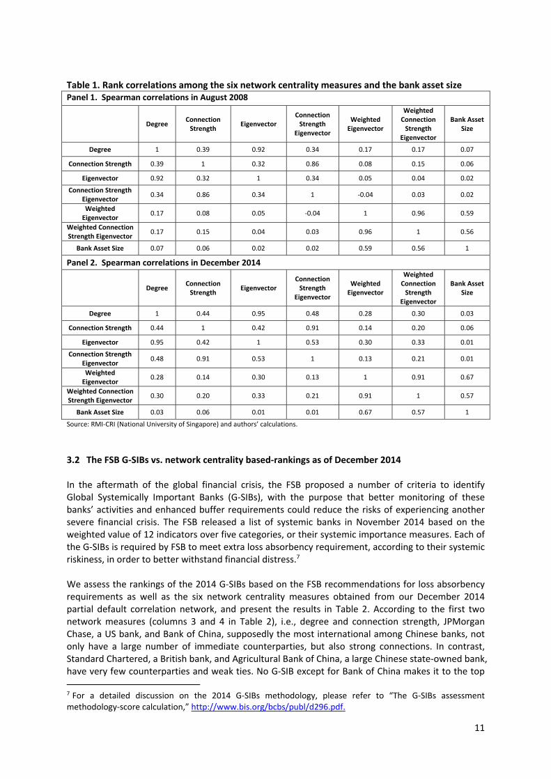
five‐year rolling data window. For the factors’ own time series dynamics, we use an expanding‐data window (i.e., all data up to the prediction time) in estimation, because the factors are broad‐based credit risk indices that need longer time series to estimate with reasonable precision.   In  the analysis  that  follows,  the  forward‐looking PDs are  for    the one‐year prediction horizon, and the PD correlation matrix is calculated for the one‐year PDs one month ahead ofthe prediction time. We conduct  the analysis  for two  time points, August 2008 and December 2014. The choice of the first time point is rather obvious, as it is right before the failure and bankruptcy of Lehman Brothers, which set off a global  financial crisis. The second point corresponds  to  the economic environment prevalent once the crisis  largely subsided. The number of banks  in the August 2008 and December 2014 samples are quite similar, 1,269 and 1,275 respectively.  The partial correlation matrices computed for August 2008 and December 2014 exhibit substantial sparsity, as zero entries account for about 97 percent of all entries  in both dates. Not surprisingly, this result is expected because, first, only direct connections are measured, and second, CONCORD, a penalty‐based method, shrinks partial correlations towards zero. Recall that our partial correlation matrix construction  increases sparsity up  to  the point  that an orphan bank begins  to emerge. Any higher sparsity will result  in some bank(s) to be totally  isolated from the global banking network  in terms of credit risk, a hardly sensible outcome.   3.1  Comparing the six network centrality measures  As section 2 noted, different centrality measures capture the relative importance of each bank in the network from different angles. To show the relations among these measures, Table 1 presents the rank correlations among the six centrality measures and the asset size for both the August 2008 and December 2014 samples. The degree centrality, which measures the number of connected parties a bank  has,  is  highly  correlated  with  the  eigenvector  centrality,  as  the  latter  factors  in  both connectedness and the extent to which its connected parties are further connected. The same thing applies to the connection strength and connection strength eigenvector centrality due to the same reason.  As  expected,  the  asset  size  is  considerably  correlated  with  the  two  bank  size‐weighted centrality measures.   Neglecting node  characteristics,  i.e.,  the  size of  the banks,  leads  to  some  surprising  and possibly counterintuitive results. In August 2008, the largest positive partial correlation is between the Bank of Nova Scotia, a Canadian Bank, and Powszechna Kasa Oszczednosci Bank Polski SA, a Polish bank, at 0.6125. As a comparison, the most negative partial correlation  is between the Peoples Financial Corp,  a US bank,  and Banco Bilbao Vizcaya Argentaria  (BBVA) Chile  SA,  the Chilean  subsidiary of Spanish bank BBVA, at  ‐0.1930. Corp Bank, an  Indian bank,  ranks  first  in  terms of  the number of connections to other banks, at 83. By contrast, Centrum Capital Ltd, an Indian bank, ranks last with only one connection to another Indian bank, Kirayaka Holdings Inc. In terms of average connection strength,  CIL  Securities  Ltd,  another  Indian  bank,  has  the  highest  strength  at  23bps,  whereas Centrum Capital Ltd has the lowest with a negligible magnitude.   In December  2014  the  largest  positive  partial  correlation  is  between  The Hyakujushi Bank  Ltd,  a Japanese bank, and Arab Jordan  Investment Bank, a Jordan‐based bank, at 0.6366, while the most negative one is between the Woori Investment Bank Co Ltd, a Korean bank, and Euro Yatirim Holding AS, a Turkish bank, at  ‐0.2524.   Royal Bancshares of Pennsylvania  Inc, a US bank, has  the highest number of connections at 83, and Banco Davivienda SA, a Colombian bank, has only one connection with  Saudi Hollandi Bank,  a  Saudi Arabian  bank. As  to  the  average  connection  strength, Bank  of China,  a  Chinese  bank,  ranks  first  at  23bps,  and  Banco  Davivienda  SA  ranks  the  lowest  with  a negligible value. 

11  

 Table 1. Rank correlations among the six network centrality measures and the bank asset size Panel 1.  Spearman correlations in August 2008

 

Degree Connection Strength 

Eigenvector Connection Strength 

Eigenvector 

Weighted Eigenvector 

Weighted Connection Strength 

Eigenvector 

Bank Asset Size 

Degree  1  0.39  0.92  0.34  0.17  0.17  0.07 

Connection Strength  0.39  1  0.32  0.86  0.08  0.15  0.06 

Eigenvector  0.92  0.32  1  0.34  0.05  0.04  0.02 

Connection Strength Eigenvector  0.34  0.86  0.34  1  ‐0.04  0.03  0.02 

Weighted Eigenvector  0.17  0.08  0.05  ‐0.04  1  0.96  0.59 

Weighted Connection Strength Eigenvector  0.17  0.15  0.04  0.03  0.96  1  0.56 

Bank Asset Size  0.07  0.06  0.02  0.02  0.59  0.56  1 

Panel 2.  Spearman correlations in December 2014 

 

Degree Connection Strength 

Eigenvector Connection Strength 

Eigenvector 

Weighted Eigenvector 

Weighted Connection Strength 

Eigenvector 

Bank Asset Size 

Degree  1  0.44  0.95  0.48  0.28  0.30  0.03 

Connection Strength  0.44  1  0.42  0.91  0.14  0.20  0.06 

Eigenvector  0.95  0.42  1  0.53  0.30  0.33  0.01 

Connection Strength Eigenvector  0.48  0.91  0.53  1  0.13  0.21  0.01 

Weighted Eigenvector  0.28  0.14  0.30  0.13  1  0.91  0.67 

Weighted Connection Strength Eigenvector  0.30  0.20  0.33  0.21  0.91  1  0.57 

Bank Asset Size  0.03  0.06  0.01  0.01  0.67  0.57  1 

Source: RMI‐CRI (National University of Singapore) and authors’ calculations. 

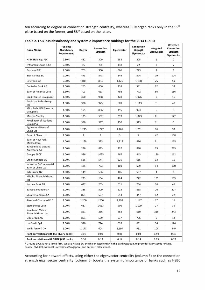
  3.2  The FSB G‐SIBs vs. network centrality based‐rankings as of December 2014  In  the  aftermath  of  the  global  financial  crisis,  the  FSB  proposed  a  number  of  criteria  to  identify Global  Systemically  Important  Banks  (G‐SIBs), with  the  purpose  that  better monitoring  of  these banks’ activities and enhanced buffer requirements could reduce the risks of experiencing another severe  financial  crisis. The  FSB  released a  list of  systemic banks  in November 2014 based on  the weighted value of 12 indicators over five categories, or their systemic importance measures. Each of the G‐SIBs is required by FSB to meet extra loss absorbency requirement, according to their systemic riskiness, in order to better withstand financial distress.7  We assess the rankings of the 2014 G‐SIBs based on the FSB recommendations for loss absorbency requirements  as well  as  the  six  network  centrality measures  obtained  from  our December  2014 partial default  correlation network, and present  the  results  in Table 2. According  to  the  first  two network measures  (columns 3  and 4  in  Table 2),  i.e., degree  and  connection  strength,  JPMorgan Chase, a US bank, and Bank of China, supposedly the most international among Chinese banks, not only have  a  large number of  immediate  counterparties, but  also  strong  connections.  In  contrast, Standard Chartered, a British bank, and Agricultural Bank of China, a large Chinese state‐owned bank, have very few counterparties and weak ties. No G‐SIB except for Bank of China makes it to the top                                                             7 For  a  detailed  discussion  on  the  2014  G‐SIBs  methodology,  please  refer  to  “The  G‐SIBs  assessment methodology‐score calculation,” http://www.bis.org/bcbs/publ/d296.pdf.  

12  

ten according to degree or connection strength centrality, whereas JP Morgan ranks only in the 95th place based on the former, and 58th based on the latter.   Table 2. FSB loss absorbency and systemic importance rankings for the 2014 G‐SIBs  

Bank Name FSB Loss 

Absorbency Requirement 

Degree Connection Strength 

Eigenvector Connection Strength 

Eigenvector 

Weighted Eigenvector 

Weighted Connection Strength 

Eigenvector 

HSBC Holdings PLC  2.50%  432  309  288  205  1  2 

JPMorgan Chase & Co  2.50%  95  58  118  22  3  7 

Barclays PLC  2.00%  703  350  566  223  2  1 

BNP Paribas SA  2.00%  473  548  649  574  19  104 

Citigroup Inc  2.00%  1,014  833  1,126  1,100  25  59 

Deutsche Bank AG  2.00%  255  656  238  541  22  33 

Bank of America Corp  1.50%  703  663  792  772  60  186 

Credit Suisse Group AG  1.50%  390  938  428  1,076  9  16 

Goldman Sachs Group Inc 

1.50%  338  975  589  1,113  31  48 

Mitsubishi UFJ Financial Group Inc 

1.50%  195  836  195  923  5  8 

Morgan Stanley  1.50%  125  532  319  1,023  61  122 

Royal Bank of Scotland Group PLC 

1.50%  390  597  450  513  11  3 

Agricultural Bank of China Ltd 

1.00%  1,215  1,247  1,161  1,251  16  93 

Bank of China Ltd  1.00%  2  1  3  2  42  108 

Bank of New York Mellon Corp 

1.00%  1,158  333  1,215  886  91  115 

Banco Bilbao Vizcaya Argentaria SA 

1.00%  296  813  237  880  73  235 

Groupe BPCE*  1.00%  526  1,025  467  843  120  112 

Credit Agricole SA  1.00%  526  544  526  615  13  15 

Industrial & Commercial Bank of China Ltd 

1.00%  125  762  169  699  14  100 

ING Groep NV  1.00%  149  586  106  597  4  6 

Mizuho Financial Group Inc 

1.00%  223  154  424  272  189  185 

Nordea Bank AB  1.00%  637  265  611  264  36  41 

Banco Santander SA  1.00%  338  509  223  818  26  207 

Societe Generale SA  1.00%  851  697  644  447  12  22 

Standard Chartered PLC  1.00%  1,260  1,260  1,198  1,147  17  11 

State Street Corp  1.00%  637  1,063  906  1,109  27  39 

Sumitomo Mitsui Financial Group Inc 

1.00%  851  366  868  510  319  243 

UBS Group AG  1.00%  801  559  637  736  6  12 

UniCredit SpA  1.00%  576  774  699  661  34  126 

Wells Fargo & Co  1.00%  1,173  604  1,199  961  108  349 

Rank correlations with FSB (1,275 banks)  0.01  0.01  0.01  0.04  0.59  0.36 

Rank correlations with SRISK (453 banks)  0.10  0.13  0.14  0.14  0.25  0.23 

* Groupe BPCE is not a listed firm. We use Natixis SA, the major listed entity in this banking group, to proxy for its systemic ranking. Source: RMI‐CRI (National University of Singapore) and authors’ calculations. 

 Accounting for network effects, using either the eigenvector centrality (column 5) or the connection strength eigenvector centrality  (column 6) boosts  the systemic  importance of banks such as HSBC 

13  

and Societe Generale, because their immediate counterparties are better/more strongly connected with others.  In contrast, Morgan Stanley and Mizuho move down the  list under eigenvector‐based centrality measures. Finally, as section 2 explained, the weighted eigenvector centrality (column 7) and weighted connection strength eigenvector centrality  (column 8), by    taking  into account both the  node  and  edge  characteristics  in  a  network  setting,  deliver  a more  comprehensive  view  of individual banks’  importance  in  the  system. Under  these  two node‐weighted  centrality measures, most of G‐SIBs  gain  a higher  systemic  ranking. Distinct  examples  include HSBC,  JPMorgan Chase, Barclays,  and  UBS  Group  AG.  In  comparison, Wells  Fargo  does  not  seem  quite  as  systemically important  as  its big‐bank peers, probably due  to  its  simple business model  and  conservative  risk taking  strategies  as  a main  street  lender, which  reduce  both  its  number  of  connections  and  the importance of connected banks.  The bottom of Table 2 presents the Spearman rank correlations between the six network centrality measures extracted  from  the  forward‐looking partial  correlation network and  two other  systemic importance  indicators.  The  first  calculation  compares  the  FSB  ranking  against  ours  for  the  1,275 banks  in  the December  2014  sample.  To  create  the  FSB  ranking, we  rank  the  30 G‐SIBs  from  1 onward, allowing for ties when multiple banks fall in the same loss absorbency basket, and assign a ranking of 31 to the remaining 1,246 banks assuming they all fall in the same and last basket.   Under  the  six  centrality measures,  on  the  other  hand,  the  highest  ranked  30  banks  keep  their genuine ranking, while the others are assigned the number 31. The Spearman coefficients  indicate that  the FSB methodology does not seem  to account much  for  the number and strength of  inter‐bank connections. As a reference, the rank correlation between the FSB indicator and the bank size, not  reported  in Table 2,  is 0.80.  It suggests  that  the FSB methodology  relies heavily on bank size, which  also  explains  the  relatively high  correlation of  the  FSB  ranking with  the  two  size‐weighted centrality measures, 0.59 and 0.36 for the weighted eigenvector and weighted connection strength eigenvector, respectively.  For  comparison  purposes,  Table  2  also  presents  the  rank  correlations  between  the  six  centrality measures and the SRISK, which we extract from the Systemic Risk Analysis of World Financials by the V‐Lab  of  the  Volatility  Institute  at  the New  York  University  Stern  School  of  Business.8 Given  the different coverage of banks in the two analyses, the comparison is conducted only for 453 banks that are both in our and V‐Lab’s samples as of December 31, 2014. The rank correlation coefficients are generally modest. This phenomenon reflects the fundamentally different approach used by the V‐lab, where co‐movements between firms are based on equity returns and depend on a single risk factor, the  broad market  equity  index.  Due  to  its  use  of  equity  returns,  the  SRISK  only  offers  indirect information about default connections. Moreover, the SRISK does not exploit the network structure fully as is the case with our systemic risk measures.        3.3  Systemic risk rankings of banks in August 2008  Performing the network analysis  in August 2008  is  interesting  in  its own right. Within the following month, the US Treasury placed Fannie Mae and Freddie Mac into conservatorship, Lehman Brothers filed for bankruptcy, Merrill Lynch sold itself to Bank of America, and the Federal Reserve bailed out AIG.  These  events  not  only  shook  the  global  financial  system  but  they  also  prompted  the  US government to implement the $700‐billion Troubled Asset Relief Program (TARP) shortly afterwards. 

                                                            8 The SRISK measure of a firm is set equal to its expected capital shortfall in a crisis scenario characterized by a 40 percent decline in the broad market index. The measure is used to rank the systemic risk of global financial firms, with the rank updated on a weekly frequency. Details are available at http://vlab.stern.nyu.edu/en/.  

14  

In  the  following  paragraphs, we will  use  our  tools  and metrics  to  help  reflect  on  some  of  these unusual occurrences.  Table 3. Systemic rankings and the total assets for New York City‐based banks, August 2008 

  Degree Connection Strength 

Eigenvector Connection Strength 

Eigenvector 

Weighted Eigenvector 

Weighted Connection Strength 

Eigenvector 

Bank Asset Size (in 

billions of USD) 

Citigroup  1,014  274  1,104  680  20  14  2,199,848 

JPMorgan Chase  12  7  14  10  391  395  1,642,862 

Goldman Sachs  287  967  464  848  152  66  1,189,006 

Morgan Stanley  287  817  118  1,167  440  607  1,090,896 

Merrill Lynch  209  157  448  525  10  8  1,042,054 

Lehman Brothers  452  355  480  206  26  25  786,035 

Bank of New York Mellon 

1,080  247  1,180  634  18  24  204,935 

Source: RMI‐CRI (National University of Singapore) and authors’ calculations. 

 Table 3 displays the systemic importance indicators for then major banks centered in New York City in August 2008. With the exception of Lehman Brothers and Merrill Lynch, these banks benefitted from  large government bailout funds. The two size‐weighted centrality measures (columns 6 and 7 in Table 3), which we believe capture better  the  systemic  risk of banks,  suggest  that among New York‐based banks,  JPMorgan Chase and Morgan Stanley do not pose a major  threat  to  the global banking system. These two firms had linkages mainly with other smaller banks. In the particular case of JPMorgan Chase, not accounting for the size of the bank and its connected counterparties would have ranked the bank among the top 20 in the world (columns 2 to 5 in Table 3).   

Figure 1. Major New York City‐centered banks and their communities, August 2008 

 

15  

Lehman Brothers, Merrill Lynch and Citigroup, one the other hand, were connected to some of the largest banks  in  the United  States and  the  rest of  the world. Although  Lehman was  smaller  than other major  investment banks when measured  in  terms of  total  assets,  its  size‐weighted  ranking among the top 30 banks  in the world did not  justify the decision to  let  it go  into bankruptcy.9 This event may have contributed to the cascading defaults of  its major counterparties  later on.  Indeed, our  data  indicates  that  among  the  32  banks  that  had  positive  partial  correlations with  Lehman Brothers  in  August  2008  analysis,  12  of  them were  subsequently  delisted  from  their  respective exchanges,  with four of the delisted banks occurring within one year of Lehman’s collapse.  Figure 1 presents the seven major New York City‐based banks, identified by their equity tickers, with their associated banking communities as of August 2008. Different colors denote  the geographical domicile of the banks and counterparts, with other major banks also identified by their equity tickers.    

The first striking feature in Figure 1 is that the community of each of the seven New York banks had very different characteristics. For  instance, Goldman Sachs and  the Bank of New York Mellon had large  counterparties.  In  the  case  of  the  former,  this  may  be  due  to  its  large  role  as  a  large correspondent bank. In contrast, Morgan Stanley was mainly connected to smaller banks domiciled in  North  America,  and  its  community  was  somewhat  isolated  from  those  of  other  banks.  The communities of  JPMorgan Chase and Lehman Brothers comprised a more diverse pool of banking counterparties  from around  the world, and  tended  to overlap with other communities. The closer banks,  in terms of overlapping communities and direct connections between them, were Citigroup and Merrill Lynch.  

 

4. Banking Networks Based on Other Correlation Measures  In  the  financial network  literature, a variety of measures has been used  to construct  the network (e.g.,  Kenett  et  al.  2010;  Demirer  et  al.  2015).  The  following  two  examples  employ  alternative measures and data, and the resulting networks can be substantially different from those obtained by using the forward‐looking PD partial default correlations.   4.1  Historical PDs vs. simulated PDs  The  first  example  compares  the  systemic measures  obtained with  the  1‐year  PDs  on  a  forward‐looking basis with  those using  the historical  time  series of 1‐year PDs obtained  from  the RMI‐CRI database. As explained earlier, the forward‐looking PDs characterize one month  later the potential default  risk of  a bank over  a 1‐year horizon. Therefore,  the partial  correlations  and  the  resulting network are  forward‐looking  in nature.  In contrast,  the historical PD  series of a  firm captures  the past  evolution  of  its  default  risk  over  time.  The  partial  correlation  of  two  series  reveals  the  co‐movement of default risk averaged over the sample period  in the past and  is therefore backward‐looking.  To construct the backward‐looking measure, we take monthly series of the RMI‐CRI 1‐year PDs from 1990  to 2014  to  form a historical  series  for each bank  in  the  sample. We  then obtain  the partial correlations among the monthly difference of each series in the sample.   One challenge in dealing with the historical PD series is that the banks  in the sample may not have the same or enough overlapping periods of observations. As a consequence,  it may be difficult  to 

                                                            9 This result supports earlier analysis based on pair‐wise interconnectedness suggesting that Lehman Brothers was too systemic to fail (Chan‐Lau, 2009, among others). 

16  

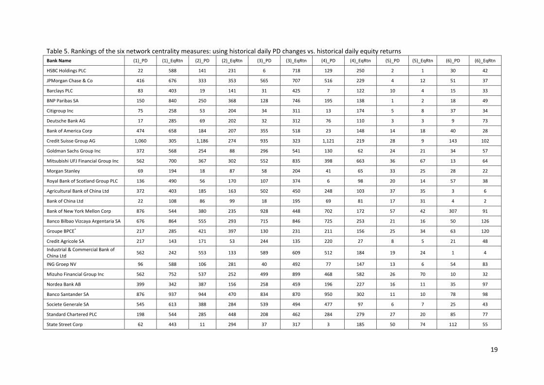
obtain  the  sample  correlation  matrix,  which  is  a  crucial  input  in  estimating  the  true  partial correlation matrix. Our solution is to compute the sample correlations in a pairwise fashion in order to make use of  the maximum number of observations  in each series. We subsequently adjust  the resulting correlation matrix element by element to render it positive semi‐definite following Qi and Sun (2011), and then convert it to a partial correlation matrix.  Table 4 compares the systemic rankings of the forward‐looking and backward‐looking networks, for the 2014 G‐SIBs. As can be seen, the two approaches yield substantially different results for each of the six network centrality measures. For the two bank size‐weighted centrality measures, forward‐looking  rankings  raise  the  importance  of  Credit  Suisse, Mitsubishi,  and UBS Group  among  other banks  relative  to  their backward‐looking  counterparts.  In  contrast,  for banks  including BNP Paris, Bank of America and Sumitomo Mitsui Financial Group, their forward‐looking systemic importance is below their average level across time. From this comparison, it is apparent that using the ‘backward‐looking’ PDs to  imply the banks’ would‐be connectedness  in the future will be quite different from relying on the forward‐looking PDs at the time of analysis.    4.2  Equity returns vs. PDs   This example  compares  the banking network  generated using equity  returns against  the network generated with historical PD series. We collect from Bloomberg historical daily equity returns for the period between 1990 and December 2014 for all banks  in our sample. As the banks  in our sample are  listed  in many exchanges  in different  countries/economies, we denominate  the  returns  in US dollar to ensure comparability. For this comparison study, we collect from the RMI‐CRI database the daily historical 1‐year PD series because daily equity returns are used. This example highlights how different  types of  risk measures  can  generate  substantially different partial  correlation networks. Table 5 reports the rankings for the six systemic importance indictors for the 2014 G‐SIBs.  It  is apparent  that rankings can differ markedly depending on whether equity returns or historical PDs  are  used.  This  is  the  case  for  the  degree  and  connection  strength  centralities.  Once  node characteristics are accounted for,  i.e., the banks’ total assets sizes, the rankings from different raw data  sources  start  to get  closer with each other.    For example,  the PD‐based bank  size‐weighted eigenvector centrality has a Spearman coefficient of 0.63 with that constructed with equity returns. This reflects in a way the important role that the node characteristics play in determining the banks’ importance in the global network.    

17  

Table 4. Rankings under the six network centrality measures: using historical PDs vs. forward‐looking PDs Bank Name  (1)_F  (1)_H  (2)_F  (2)_H  (3)_F  (3)_H  (4)_F  (4)_H  (5)_F  (5)_H  (6)_F  (6)_H 

HSBC Holdings PLC  432  80  309  720  288  140  205  575  1  2  2  6 

JPMorgan Chase & Co  95  870  58  1,067  118  1,038  22  1,074  3  1  7  23 

Barclays PLC  703  676  350  517  566  666  223  584  2  13  1  69 

BNP Paribas SA  473  393  548  706  649  353  574  684  19  3  104  2 

Citigroup Inc  1,014  393  833  524  1,126  608  1,100  623  25  4  59  72 

Deutsche Bank AG  255  561  656  721  238  710  541  722  22  11  33  59 

Bank of America Corp  703  975  663  561  792  890  772  686  60  10  186  53 

Credit Suisse Group AG  390  1,253  938  1,063  428  1,266  1,076  1,235  9  324  16  642 

Goldman Sachs Group Inc  338  919  975  848  589  1,055  1,113  1,011  31  7  48  70 

Mitsubishi UFJ Financial Group Inc  195  676  836  796  195  635  923  759  5  83  8  154 

Morgan Stanley  125  346  532  511  319  535  1,023  693  61  20  122  73 

Royal Bank of Scotland Group PLC  390  181  597  135  450  282  513  321  11  26  3  123 

Agricultural Bank of China Ltd  1,215  80  1,247  160  1,161  243  1,251  29  16  459  93  795 

Bank of China Ltd  2  783  1  866  3  695  2  560  42  73  108  219 

Bank of New York Mellon Corp  1,158  1,093  333  678  1,215  1,195  886  1,115  91  890  115  1,021 

Banco Bilbao Vizcaya Argentaria SA  296  1,012  813  927  237  1,052  880  1,166  73  29  235  40 

Groupe BPCE*  526  676  1,025  977  467  795  843  860  120  19  112  4 

Credit Agricole SA  526  512  544  465  526  548  615  690  13  6  15  1 

Industrial & Commercial Bank of China Ltd 

125  284  762  666  169  378  699  555  14  305  100  245 

ING Groep NV  149  346  586  331  106  543  597  540  4  44  6  82 

Mizuho Financial Group Inc  223  512  154  597  424  428  272  672  189  96  185  196 

Nordea Bank AB  637  618  265  879  611  760  264  859  36  9  41  32 

Banco Santander SA  338  1,246  509  1,158  223  1,213  818  1,221  26  25  207  18 

Societe Generale SA  851  727  697  239  644  1,002  447  956  12  5  22  57 

Standard Chartered PLC  1,260  676  1,260  964  1,198  845  1,147  955  17  77  11  140 

State Street Corp  637  229  1,063  127  906  221  1,109  273  27  195  39  272 

Sumitomo Mitsui Financial Group  851  393  366  322  868  259  510  600  319  78  243  173 

18  

Inc 

UBS Group AG  801  727  559  520  637  746  736  589  6  381  12  343 

UniCredit SpA  576  452  774  615  699  529  661  534  34  12  126  43 

Wells Fargo & Co  1,173  727  604  445  1,199  770  961  530  108  490  349  521 

Notes:  1.  The  column  numbers  are:  (1)  degree  centrality,  (2)  connection  strength  centrality,  (3)  eigenvector  centrality,  (4)  eigenvector  connection  strength  centrality,  (5)  TA‐weighted eigenvector centrality, (6) TA‐weighted eigenvector connection strength centrality.  2. ‘_H’ means results derived from the historical PD series. ‘_F’ denotes results derived from the forward‐looking PDs. * Groupe BPCE is not a listed firm. We use Natixis SA, the major listed entity in this banking group, to proxy for its systemic ranking. 

   

                 

19  

Table 5. Rankings of the six network centrality measures: using historical daily PD changes vs. historical daily equity returns Bank Name  (1)_PD  (1)_EqRtn  (2)_PD  (2)_EqRtn  (3)_PD  (3)_EqRtn  (4)_PD  (4)_EqRtn  (5)_PD  (5)_EqRtn  (6)_PD  (6)_EqRtn 

HSBC Holdings PLC  22  588  141  231  6  718  129  250  2  1  30  42 

JPMorgan Chase & Co  416  676  333  353  565  707  516  229  4  12  51  37 

Barclays PLC  83  403  19  141  31  425  7  122  10  4  15  33 

BNP Paribas SA  150  840  250  368  128  746  195  138  1  2  18  49 

Citigroup Inc  75  258  53  204  34  311  13  174  5  8  37  34 

Deutsche Bank AG  17  285  69  202  32  312  76  110  3  3  9  73 

Bank of America Corp  474  658  184  207  355  518  23  148  14  18  40  28 

Credit Suisse Group AG  1,060  305  1,186  274  935  323  1,121  219  28  9  143  102 

Goldman Sachs Group Inc  372  568  254  88  296  541  130  62  24  21  34  57 

Mitsubishi UFJ Financial Group Inc  562  700  367  302  552  835  398  663  36  67  13  64 

Morgan Stanley  69  194  18  87  58  204  41  65  33  25  28  22 

Royal Bank of Scotland Group PLC  136  490  56  170  107  374  6  98  20  14  57  38 

Agricultural Bank of China Ltd  372  403  185  163  502  450  248  103  37  35  3  6 

Bank of China Ltd  22  108  86  99  18  195  69  81  17  31  4  2 

Bank of New York Mellon Corp  876  544  380  235  928  448  702  172  57  42  307  91 

Banco Bilbao Vizcaya Argentaria SA  676  864  555  293  715  846  725  253  21  16  50  126 

Groupe BPCE*  217  285  421  397  130  231  211  156  25  34  63  120 

Credit Agricole SA  217  143  171  53  244  135  220  27  8  5  21  48 

Industrial & Commercial Bank of China Ltd 

562  242  553  133  589  609  512  184  19  24  1  4 

ING Groep NV  96  588  106  281  40  492  77  147  13  6  54  83 

Mizuho Financial Group Inc  562  752  537  252  499  899  468  582  26  70  10  32 

Nordea Bank AB  399  342  387  156  258  459  196  227  16  11  35  97 

Banco Santander SA  876  937  944  470  834  870  950  302  11  10  78  98 

Societe Generale SA  545  613  388  284  539  494  477  97  6  7  25  43 

Standard Chartered PLC  198  544  285  448  208  462  284  279  27  20  85  77 

State Street Corp  62  443  11  294  37  317  3  185  50  74  112  55 

20  

Sumitomo Mitsui Financial Group Inc 

242  727  263  237  216  769  324  525  23  27  11  51 

UBS Group AG  116  568  168  280  79  480  121  159  9  15  31  100 

UniCredit SpA  316  789  312  607  345  661  235  199  15  17  47  26 

Wells Fargo & Co  37  403  84  223  78  354  65  191  22  19  87  13 

Notes:  1.  The  column  numbers  are:  (1)  degree  centrality,  (2)  connection  strength  centrality,  (3)  eigenvector  centrality,  (4)  eigenvector  connection  strength  centrality,  (5)  TA‐weighted eigenvector centrality, (6) TA‐weighted eigenvector connection strength centrality.   2. ‘_PD’ means results derived from the historical daily PD series. ‘_EqRtn’ denotes results derived from the series of the historical daily equity returns. * Groupe BPCE is not a listed firm. We use Natixis SA, the major listed entity in this banking group, to proxy for its systemic ranking. 

21  

5. Conclusion  The recent financial crisis has highlighted the need to identify the systemic risk in the global financial network and to design policy measures capable of containing potential system‐wide distress. In this paper, we devise  a new methodology  for  constructing  a  global banking network  and  ranking  the systemic importance of the banks in the network.  We implement the methodology on a sample of more than one thousand public banks which literally covers all exchange‐listed banks worldwide.   Methodology‐wise, we use the default correlation model of Duan and Miao  (2015) to generate by simulation banks’ forward‐looking PD correlation matrix over a future time horizon. To disentangle the direct linkages between any bank pair from the effects of other banks in the global network, we apply the CONCORD algorithm of Khare et al. (2015) to transform the forward‐looking PD correlation matrix into a partial correlation matrix. We then apply the concept of network centrality to create six measures  of  systemic  importance.  Apart  from  the  simple  connectedness  indicators,  we  use eigenvector centrality measures to capture the  importance of a bank based on  its connections and how  its  connected parties  are  further  connected. Two of  the measures use both  the node  (bank asset size) and edge characteristics to construct the systemic importance. To graphically present the global banking network, we use  the  tool Gephie  to partition  the network  into bank/group centric communities.   With this methodology, we analyze the banking networks at the height of the global financial crisis in 2008 as well at  the end of 2014 when  the  crisis has  subsided. Our  systemic  importance  rankings suggest that Lehman Brothers was more systemically importance than what the US authorities then thought. We also show that our rankings are substantially different from other alternatives, such as the FSB G‐SIBs. Among our systemic risk measures, the ones factoring  in both edge (partial default correlation) and node characteristic (bank size) are closer to the FSB rankings.    

References 1. Acharya, V., Engle, R. & Richardson, M., 2012,  "Capital  Shortfall: A New Approach  to 

Ranking  and  Regulating  Systemic  Risks,"  American  Economic  Review,  Papers  and Proceedings  of  the  One  Hundred  Twenty  Fourth  Annual  Meeting  of  the  American Economic Association, 102(3), pp. 59‐64. 

2. Adrian, T. and Brunnermeier, M.K., 2014, "CoVar," Federal Reserve Bank of New York Staff Reports, No. 348. 

3. Bailey,  N.,  Kapetanios,  G.,  and  Pesaran,  M.,  2015a,  "Exponent  of  Cross‐Sectional Dependence: Estimation and Inference," Journal of Applied Econometrics, forthcoming. 

4. Bailey,  N.,  Holly,  S.,  and  Pesaran,  M.,  2015b,  "A  Two  Stage  Approach  to  Spatial‐Temporal  Analysis  with  Strong  and  Weak  Cross‐Sectional  Dependence,"  Journal  of Applied Econometrics, forthcoming. 

5. Barigozzi, M. and Brownlees, C., 2016, "Nets: Network Estimation for Time Series," SSRN.  6. Basel  Committee  on  Banking  Supervision,  Nov.  2014,  "The  G‐SIB  assessment 

methodology‐score calculation."  7. Basel Committee on Banking Supervision, 2013, "Global Systemically  Important Banks: 

Updated  Assessment  Methodology  and  the  Higher  Loss  Absorbency  Requirement (Basel)." 

8. Billio,  M.,  Getmansky,  M.,  Gray,  D.,  Lo,  A.,  Merton,  R.C.,  and  Pelizzon,  L.,  2013, "Sovereign, Bank, and Insurance Credit Spreads Connectedness and System Networks," mimeo (Massachusetts Institute of Technology). 

22  

9. Billio, M.,  Getmansky, M.,  Lo,  A.,  and  Pelizzon,  L.,  2012,  "Econometric Measures  of Connectedness  and  Systemic  Risk  in  the  Finance  and  Insurance  Sectors,"  Journal  of Financial Economics, Vol. 104, pp. 535 ‐ 559. 

10. Brownlees, C.T., and Engle, R.F., 2015, "SRISK: A Conditional Capital Shortfall Measures of Systemic Risk," mimeo (Universitat Pompeu Fabra and New York University). 

11. Canova, F., and Ciccarelli, M., 2013,  "Panel Vector Autoregressive Models: a Survey," Working Paper Series 1507 (European Central Bank). 

12. Chan‐Lau, J.A., 2013, Systemic Risk Assessment and Oversight, Risk Books. 13. Chan‐Lau, J.A., 2009, "Default Risk Codependence  in the Global Financial System: Was 

the Bear Stearns Bailout Justified?, in G. Gregoriou, editor, The Banking Crisis Handbook (McGraw Hill). 

14. Chudik,  A.,  Pesaran,  M.,  and  Tosetti,  E.,  2011,  "Weak  and  Strong  Cross  Section Dependence and Estimation of Large Panels," Econometrics Journal, Vol. 14, No. 1, pp. C45 ‐ C90. 

15. Craig,  B.,  and  Saldias, M.,  2016,  "Spatial  Dependence  and  Data‐Driven  Networks  of International  Banks,"  mimeo,  Federal  Reserve  Bank  of  Cleveland  and  International Monetary Fund. 

16. Demekas, D.,  Chan‐Lau,  J.A.,  Rendak, N., Ohnsorghe,  F.,  Youssef,  K.,  Caceres,  C.  and Tintchev,  K.,  2013,  "Mandatory  Financial  Stability  Assessments  under  the  Financial Sector Assessment Program: Update," International Monetary Fund (Washington, D.C.). 

17. Demirer, M., Diebold, F.X., Liu, L. and Yilmaz, K., 2015, "Estimating Global Bank Network Connectedness," Working paper. 

18. Diebold,  F.X.,  and  Yilmaz,  K.,  2014,  "On  the  Network  Topology  of  Variance Decompositions:  Measuring  the  Connectedness  of  Financial  Firms,"  Journal  of Econometrics, Vol. 182, No. 1, pp. 119 ‐134. 

19. Duan,  J.‐C.  and  Miao,  W.,  2015,  "Default  Correlations  and  Large‐Portfolio  Credit Analysis,"  Journal  of  Business  and  Economic  Statistics. (DOI:10.1080/07350015.2015.1087855) 

20. Duan,  J.‐C.,  Sun,  J.  and Wang, T., 2012,  "Multiperiod Corporate Default Prediction: A Forward Intensity Approach," Journal of Econometrics, 170(1), pp. 191‐209. 

21. Duan,  J.‐C.  and  Zhang,  C.,  2013,  "Cascading Defaults  and  Systemic  Risk  of  a  Banking Network," National University of Singapore working paper.  

22. Fan, J., 1997, "Comments on `Wavelets in Statistics: A Review' by A. Antoniadis," Journal of the Italian Statistical Society, 6(2), pp. 131‐138. 

23. Ferson,  W.  E.,  2003,  "Tests  of  Multifactor  Pricing  Models,  Volatility  Bounds,  and Portfolio Performance," Chapter 12 in G. Constantinides, M. Harris, and R. Stulz, editors, Handbook of the Economics of Finance, Vol. 1A, pp. 743 ‐ 802. 

24. Fiedler,  M.,  1973,  "Algebraic  Connectivity  of  Graphs,"  Czechoslovak  Mathematical Journal, 23(2), pp. 298‐305.  

25. Financial Stability Board, 2014,  "2014 Update of  List of Global Systemically  Important Banks (G‐SIBs) (Basel)." 

26. Girvan, M. and Newman, M. E. J., 2002, "Community Structure  in Social and Biological Networks,"  Proceedings  of  the National Academy  of  Sciences  of  the United  States  of America, 99(12), 7821‐7826.  

27. Huang, X., Zhou, H. and Zhu, H., 2009, "A Framework for Assessing the Systemic Risk of Major Financial Institutions," Journal of Banking & Finance, Vol. 33, pp. 2036‐2049. 

28. International Monetary Fund, 2009, Global Financial Stability Report (April). 

23  

29. Jacomy,  M.,  Venturini,  T.,  Heymann,  S.  and  Bastian,  M.,  2014,  "ForceAtlas2,  A Continuous Graph Layout Algorithm for Handy Network Visualization Designed for the Gephi Software," PLOS One.  

30. Kenett,  Dror  Y.,  Tumminello, M., Madi,  A., Gur‐Gershgoren, G., Mantegna,  R.N.  and Ben‐Jacob,  E.,  2010,  "Dominating  Clasp  of  the  Financial  Sector  Revealed  by  Partial Correlation Analysis of the Stock Market," PlOS One. 

31. Kernighan,  B. W.  and  Lin,  S.,  1970,  "An  Efficient Heuristic  Procedure  for  Partitioning Graphs," Bell System Technical Journal, 49(2), pp. 291‐307.  

32. Khare, K., Oh, S.‐Y. and Rajaratnam, B., 2015, "A Convex Pseudo‐likelihood Framework for  High  Dimensional  Partial  Correlation  Estimation  with  Convergence  Guarantees," Journal of the Royal Statistical Society: Series B (Statistical Methodology), pp. 803‐825. 

33. Koop, G., Pesaran, M., and Potter,  S., 1996,  "Impulse Response Analysis  in Nonlinear Multivariate Models," Journal of Econometrics, Vol. 74, pp. 119 ‐ 147. 

34. Lanne, M., and Nyberg, H., 2016, "Generalized Forecast Error Variance Decomposition for  Linear  and  Nonlinear  Multivariate  Models,"  forthcoming  in  Oxford  Bulletin  of Economics and Statistics. 

35. Mantegna, R. N., 1999, "Hierarchical Structure in Financial Markets," European Physical Journal B ‐ Condensed Matter and Complex Systems, Volume 1, pp. 193 ‐ 197.  

36. Oh,  S.‐Y.,  Dalal,  O.,  Khare,  K.  and  Rajaratnam,  B.,  2014,  "Optimization Methods  for Sparse  Pseudo‐likelihood  Graphical  Model  Selection,"  Appeared  in  conference proceedings for 'Neural Information Processing System 2014'. 

37. Pothen,  A., Simon,  H.  D.,  and Liou  K‐P.,  1990,  "Partitioning  Sparse  Matrices  with Eigenvectors of Graphs," Siam  Journal on Matrix Analysis and Applications, 11(3), pp. 430‐452.  

38. Palla,  G.,  Derenyi,  I.,  Farkas,  I.  and  Vicsek,  T.,  2005,  "Uncovering  the  Overlapping Community  Structure  of  Complex Networks  in Nature  and  Society," Nature  435,  pp. 814‐818. 

39. Patro, D. K., Qi, M. and Sun, X., 2013, "A Simple Indicator of Systemic Risk," Journal of Financial Stability, pp. 105‐116. 

40. Peng,  J., Wang, P., Zhou, N. and Zhu,  J., 2009, "Partial Correlation Estimation by  Joint Sparse Regression Models," Journal of the American Statistical Association, 104(486). 

41. Pesaran,  H.,  and  Shin,  Y.,  1998,  "Generalized  Impulse  Response  Analysis  in  Linear Multivariate Models," Economics Letters, Vol. 58, pp. 17 ‐ 29. 

42. Qi, H. and Sun, D., 2011, "An Augmented Lagrangian Dual Approach for the H‐weighted Nearest Correlation Matrix Problem,"  IMA  Journal of Numerical Analysis, Vol. 31, pp. 491‐511. 

43. RMI‐CRI,  2015,  "NUS‐RMI  Credit  Research  Initiative  Technical  Report  Version:  2015 Update 1," Global Credit Review, Vol. 5. 

44. Scott, J., 2000, Social Network Analysis: A Handbook, 2nd edition, Thousand Oaks, CA: Sage Publications. 

45. Tumminello,  M.,  Lillo,  F.  and  Mantegna,  R.,  2010,  "Correlation,  Hierarchies,  and Networks in Financial Markets," Journal of Economic Behavior & Organization, pp. 40‐58. 

46. Xie,  J.,  S.  Kelley,  and  B.K.  Szymanski,  2014,  "Overlapping  Community  Detection  in Network: the State of the Art and Comparative Study," ACM Computing Surveys, Vol. 45, No. 4.