WP/06/297

Bank Risk-Taking and Competition Revisited: New Theory and New Evidence

John H. Boyd, Gianni De Nicolò, and

Abu M. Jalal

© 2006 International Monetary Fund WP/06/297 IMF Working Paper Research Department

Bank Risk-Taking and Competition Revisited: New Theory and New Evidence

Prepared by John H. Boyd, Gianni De Nicolò, and Abu M. Jalal1

Authorized for distribution by Laura Kodres

December 2006

Abstract This Working Paper should not be reported as representing the views of the IMF. The views expressed in this Working Paper are those of the author(s) and do not necessarily represent those of the IMF or IMF policy. Working Papers describe research in progress by the author(s) and are published to elicit comments and to further debate.

This paper studies two new models in which banks face a non-trivial asset allocation decision. The first model (CVH) predicts a negative relationship between banks’ risk of failure and concentration, indicating a trade-off between competition and stability. The second model (BDN) predicts a positive relationship, suggesting no such trade-off exists. Both models can predict a negative relationship between concentration and bank loan-to-asset ratios, and a nonmonotonic relationship between bank concentration and profitability. We explore these predictions empirically using a cross-sectional sample of about 2,500 U.S. banks in 2003 and a panel data set of about 2,600 banks in 134 nonindustrialized countries for 1993-2004. In both these samples, we find that banks’ probability of failure is positively and significantly related to concentration, loan-to-asset ratios are negatively and significantly related to concentration, and bank profits are positively and significantly related to concentration. Thus, the risk predictions of the CVH model are rejected, those of the BDN model are not, there is no trade-off between bank competition and stability, and bank competition fosters the willingness of banks to lend.

JEL Classification Numbers: G21, G32, L13 Keywords: Bank Competition, Concentration, Risk, Asset Allocations Author’s E-Mail Address: gdenicolo@imf.org; JBoyd@csom.umn.edu; AJalal@csom.umn.edu

1 Boyd and Jalal are with the Carlson School, University of Minnesota. De Nicolò is with the IMF Research Department. We thank Gordon Phillips, Ross Levine, Douglas Gale, Itam Goldstein, Charles Goodhart, Bilal Zia, and seminar participants at the Federal Reserve Bank of Atlanta, the University of Colorado, the European Central Bank, the Bank of Italy, the London School of Economics, Mannheim University, 2006 Summer Finance Conference, Said School, Oxford University, the 2006 Summer Asset Pricing Meetings, NBER, and the JFI-World Bank Conference on Bank Regulation and Corporate Finance , Washington D.C., for comments and suggestions.

2

Contents Page I. Introduction ........................................................................................................................3 II. Theory ........................................................................................................................5 A. The CVH Model....................................................................................................5 B. The BDN Model..................................................................................................11 C. Summary .............................................................................................................18 III. Evidence ......................................................................................................................19 A. Results for the U.S. Sample ................................................................................21 B. Results for the International Sample ...................................................................25 C. Concentration and Profits....................................................................................28 IV. Conclusion .....................................................................................................................29 Appendix I: Pareto Dominant Equilibria .............................................................................31 References............................................................................................................................48 Tables 1. U.S. Sample .............................................................................................................33 2. Simple Correlations: U.S. Sample ...........................................................................34 3. U.S. Regressions: Dependent Variable: Z ...............................................................35 4. U.S. Regressions: Dependent Variable: ROA .........................................................36 5. U.S. Regressions: Dependent Variable: EA_cox.....................................................37 6. U.S. Regressions: Dependent Variable Ln(σ(ROA)) ..............................................38 7. U.S. Regressions: Dependent Variable: LA.cox......................................................39 8. International Sample ................................................................................................40 9. Correlations: International Sample ..........................................................................41 10. International Regressions: Dependent Variable: Z-score(t) ....................................42 11. International Regressions: Dependent Variable: Components of the Z-score.........43 12. International Regressions: Dependent Variable: LA_Cox(t)...................................44 13. Regressions: Dependent Variable: LPROFIT..........................................................45 Figures 1. CVH Model (A=0.1, beta=1,r=1.1) .........................................................................46 2. CVH Model (A=0.1, beta=5,r=1.1) .........................................................................46 3. BDN Model (A=0.1, alpha=0.5, beta=2, r=1.1) ......................................................46 4. CVH Model (A=0.1, beta=5,r=1.1), Pareto Dominant Equilibrium........................47 5. BDN Model (A=0.1, alpha=0.5,beta=2,r=1.1), Pareto Dominant Equilibrium.......47

3

I. INTRODUCTION

It has been a widely-held belief among policymakers that more competition in banking is associated, ceteris paribus, with greater instability (more failures). Since bank failures are almost universally associated with negative externalities, this has been seen as a social cost of “too much competition in banking.” Yet, the existing empirical evidence on this topic is mixed and, theory, too, has produced conflicting predictions. In this paper we investigate this important policy issue bringing to bear new theory and new evidence. Our previous work (Boyd and De Nicolò, 2005) reviewed the existing theoretical research on this topic and concluded that it has had a profound influence on policymakers, both at central banks and at international agencies. We next demonstrated that the conclusions of previous theoretical research were fragile, depending on the assumption that competition is only allowed in deposit markets but suppressed in loan markets. A critical question in such models is whether banks’ asset allocation decisions are best modeled as a “portfolio allocation problem” or as an “optimal contracting problem.” By “portfolio allocation problem,” we mean a situation in which the bank allocates its assets to a set of financial claims, taking all return distributions as parametric. Purchasing some quantity of government bonds would be an example. By “optimal contracting problem,” we mean a situation in which there is private information and borrowers’ actions will depend on loan rates and other lending terms. Realistically, we know that banks are generally involved in both kinds of activity simultaneously. They acquire bonds and other traded securities in competitive markets in which there is essentially no private information and in which they are price takers. At the same time, they make many different kinds of loans in imperfectly competitive markets with private information. Therefore, it should be useful to consider an environment in which both kinds of activity can occur simultaneously. That is what is done here. We study two new banking models in which a nontrivial bank asset allocation decision is introduced by allowing banks to invest in a riskless asset, called a bond. The first model has its roots in earlier work by Allen and Gale (2000, 2004) (hereafter the “CVH” or “charter value hypothesis” model), and mirrors the modeling environment presented in several other studies (e.g. Keeley, 1990; Hellman, Murdoch and Stiglitz, 2000; and Repullo, 2004). It allows for competition in deposit, but not in loan, markets, and there is no contracting problem between banks and borrowers. The second builds on the work of Boyd and De Nicolò (2005) (hereafter the BDN model). It allows for competition in both loan and deposit markets, and banks solve an optimal contracting problem with their borrowers. Allowing banks to hold risk-free bonds results in considerable increased complexity but yields a rich new set of predictions. First, when the possibility of investing in riskless bonds is introduced, banks’ investment in bonds can be viewed as a choice of “collateral.” When bond holdings are sufficiently large, deposits become risk free.

4

Second, the asset allocation between bonds and loans becomes a strategic variable, since changes in the quantity of loans will change the return on loans relative to the return on bonds. Third, the new theoretical environments produce an interesting prediction that is invisible unless both loan and bond markets are modeled simultaneously. A bank’s optimal quantity of loans, bonds and deposits will depend on the degree of competition it faces. Thus, the banking industry’s optimal portfolio choice will depend on the degree of competition. Now, such a relationship is of more than theoretical interest. One of the key economic contributions of banks is believed to be their role in efficiently intermediating between borrowers and lenders in the sense of Diamond (1984) or Boyd and Prescott (1986). But banks would play no such role if they just raised deposit funds and used them to acquire risk-free bonds. Thus, if competition affects banks’ choices between loans and risk-free investments, that is almost sure to have welfare consequences. To our knowledge, this margin has not been recognized or explored elsewhere in the literature. The two new models yield opposite predictions with respect to banks’ risk-taking, but similar predictions with respect to portfolio allocations. The CVH model predicts a positive relationship between the number of banks and banks’ risk of failure. The BDN model predicts a negative relationship. By contrast, both models can predict that banks will allocate relatively larger amounts of total assets to lending as competition increases.

Both models have an additional implication that is new and potentially important. It is that the relationship between bank competition and profitability can easily be nonmonotone. For example, as the number of banks in a market increases, it is possible that either profits per bank or profits scaled by assets are first increasing over some range, and then decreasing thereafter. This theoretical finding casts doubts on the relevance of results of empirical studies that have assumed a priori that the theoretically expected relationship is monotonic.

We explore the predictions of the two models empirically using two data sets: a cross-sectional sample of about 2,500 U.S. banks in 2003, and an international panel data set with bank-year observations ranging from 13,000 to 18,000 in 134 nonindustrialized countries for the period 1993-2004. We present a set of regressions relating measures of concentration to measures of risk of failure, and to loan-to-asset ratios. The main results with the two different samples are qualitatively identical. First, banks’ probability of failure is positively and significantly related to concentration, ceteris paribus. Thus, the risk implications of the CVH model are not supported by the data, while those of the BDN model are. Second, the loan to asset ratio is negatively and significantly associated with concentration. This result is broadly consistent with the predictions of both models. Finally, we find that in our empirical tests bank profits are monotonically increasing in concentration with both data sets. This finding is consistent with the conventional wisdom, and with some but not all other empirical investigations.

The remainder of the paper is composed of three sections. Section II analyzes the CVH and the BDN models. Section III presents the evidence. Section IV concludes, discussing the implications of our findings for further research.

5

II. THEORY

In the next two subsections we describe and analyze the CVH and BDN models. The last subsection summarizes and compares the results for both models.

A. The CVH Model

We modify Allen and Gale’s (2000, 2004) model with deposit market competition by allowing banks to invest in a risk-free bond that yields a gross rate 1r ≥ .

The economy lasts two dates: 0 and 1. There are two classes of agents, N banks and depositors, and all agents are risk-neutral. Banks have no initial resources. They can invest in bonds, and also have access to a set of risky technologies indexed by S. Given an input level y, the risky technology yields Sy with probability p(S) and 0 otherwise. We make the following

Assumption 1 :[ , ] [0,1]p S S a satisfies: (a) ( ) ( )1, 0, 0p S p S p′= = < and 0p′′ ≤ for all ( ),S S S∈ , and

(b) ( )* *p S S r> Condition 1(a) states that ( )p S S is a strictly concave function of S and reaches a maximum *S when ( ) ( )* * * 0p S S p S′ + = . Given an input level y, increasing S from the

left of *S entails increases in both the probability of failure and expected return. To the right of *S , the higher S, the higher is the probability of failure and the lower is the expected return. Condition 1(b) states that the return in the good state (positive output) associated with the most efficient technology is larger than the return on bonds: The bank’s (date 0) choice of S is unobservable to outsiders. At date 1, outsiders can only observe and verify at no cost whether the investment’s outcome has been successful (positive output) or unsuccessful (zero output). By assumption, deposit contracts are simple debt contracts. In the event that the investment outcome is unsuccessful, depositors are assumed to have priority of claims on the bank’s assets, given by the total proceeds of bond investment, if any.

The deposits of bank i are denoted by iD , and total deposits by1

Nii

Z D=

≡ ∑ . Deposits are insured, so that their supply does not depend on risk, and for this insurance banks pay a flat rate deposit insurance premium standardized to zero. Thus, the inverse supply of deposits is denoted with ( )D Dr r Z= ,2 with 2 If bank deposits provide a set of auxiliary services (e.g. payment services, option to withdraw on demand, etc.) and depositors can invest their wealth at no cost in the risk-free asset, then deposits and “bond” holdings can be viewed as imperfect substitutes and deposits may be held even though bonds dominate deposits in rate of return.

6

Assumption 2. 0, 0D Dr r′ ′′> ≥ .

Banks are assumed to compete for depositors à la Cournot. In our two-period context, this assumption is fairly general. As shown by Kreps and Scheinkman (1983), the outcome of this competition is equivalent to a two-stage game where in the first stage banks commit to invest in observable “capacity” (deposit and loan service facilities, such as branches, ATM, etc.), and in the second stage they compete in prices.

Under this assumption, each bank chooses the risk parameter S , the investment in the technology L , bond holdings B and deposits D that are the best responses to the strategies of other banks. Let i jj i

D D− ≠≡∑ denote total deposit choices of all banks

except bank i . Thus, a bank chooses the four-tuple ( ) 2, , , 0,S L B D S xR+⎡ ⎤∈ ⎣ ⎦ to maximize:

( )( ) ( )( ) (1 ) max{0, ( ) }D i D ip S SL rB r D D D p S rB r D D D− −+ − + + − − + (1.a)

subject to L B D+ = (2.a)

As it is apparent by inspecting objective (1.a), banks can be viewed as choosing between two types of strategies. The first one results in max{.} 0> . In this case there is no moral hazard and deposits become risk free. The second one results in max{.} 0= . In this case there is moral hazard and deposits are risky. Of course, banks will choose the strategy that yields the highest expected profit. We describe each strategy in turn.

No-moral-hazard (NMH) strategy If ( )D irB r D D D−≥ + , banks’ investment in bonds is sufficiently large to pay depositors all their promised deposit payments. Equivalently, a positive investment in bonds may be viewed as a choice of “collateral”. In this case, banks may “voluntarily” provide insurance to depositors in the bad state and give up the opportunity to exploit the option value of limited liability (and deposit insurance). Under this strategy, a bank chooses ( ) 3, , , 0,S L B D S xR+⎡ ⎤∈ ⎣ ⎦ to maximize:

( ) ( )D ip S SL rB r D D D−+ − + (3.a) subject to (2.a) and

( )D irB r D D D−≥ + . (4.a)

It is evident from (3.a) that the optimal value of the risk parameter is *S , i..e., the one that maximizes ( )p S S . In other words, banks will choose the level of risk that would be chosen under full observability of technology choices. Thus, a bank chooses ( ) 3, , 0,L B D S xR+⎡ ⎤∈ ⎣ ⎦ 0L ≥ to maximize:

7

( )* *( ( ( ))D ip S S L rB r r D D D−+ + − + (5.a) subject to (2.a) and (4.a).

Substituting (2.a) in (5.a), it is evident that the objective function is strictly increasing (decreasing) in L (in B ). Thus, (4.a) is satisfied at equality, yielding optimal solutions for loans and bonds given by

* ( ) /D iB r D D D r−= + and * ( )(1 )D ir D DL Dr− +

= − . (6.a)

In sum, when banks pre-commit to the risk choice *S , at the same time they minimize the amount of bond holdings necessary to make deposits risk-free. By Assumption 2(a) (the expected return on the most efficient technology is strictly greater than the return on bonds), it is optimal for a bank to set L at the maximum level consistent with constraints (2.a) and (4.a). Furthermore, substituting (6.a) in (5.a), and differentiating the resulting objective with respect to D , the optimal level of deposits, denoted by *D , satisfies:

* * *( ) ( ) 0D i D ir r D D r D D D− −′− + − + = (7.a)

Substituting (7.a) into the objective function, the profits achieved by a bank under the NMH strategy are given by:

* *

* * *2( )( ) ( )i D ip S SD r D D D

r− −′Π ≡ + (8.a)

Finally, observe that the profit obtained by investing in bonds only ( B D= ) are given by

* *2( )D ir D D D−′ + . By Assumption 1(b) this profit is always lower than the profit in (8.a). Therefore, banks will never invest only in bonds. Denote with (.) /L Dα ≡ the loan to asset ratio, and let the four-tuple

* * * *{ , ( ), ( ), ( )}i i iS L D D D Dα− − − denote the best-response functions of a bank when the NMH strategy is chosen. The following Lemma summarizes the properties of optimal choices and profits.

Lemma 1 (a) *

0i

dLdD−

< ; (b) *

0i

ddDα

−

< ; (c) *

1 0i

dDdD−

− < < ;

(d) * * *

* *( ) ( ) 0D ii

d p S S r D D DdD r −

−

Π ′= − + < .

Proof: Differentiation of conditions (4.a) and (7.a) at equality, and application of the Envelope Theorem.

8

Moral-hazard (MH) strategy If ( )D irB r D D D−< + , banks choose a bond investment level that is insufficient to pay depositors their promised deposit payments whenever the bad state (zero output) occurs. In contrast to the previous case, banks exploit the option value of limited liability (and deposit insurance), and therefore, there is moral hazard.

Now, a bank chooses the triplet ( ) 3, , [0, ]S L D S xR+∈ to maximize:

( ) (( ) ( ( )) )D ip S S r L r r D D D−− + − + (9.a)

subject to (2.a) and ( )D irB r D D D−< + (10.a)

Substituting (2.a) in (9.a), and differentiating (9.a) with respect to S , the optimal level of risk, denoted by S% , satisfies

( ) ( ( ( )) ) ( ) 0D ip S SL rL r r D D D p S L−′ − + − + + =% % % . (11.a)

Rearranging (11.a), it can be easily verified that ( ) ( ) 0p S S p S′ + <% % % for any ( ) 2,L D R++∈ .

Hence, *S S>% by the strict concavity of the function ( )p S S . Since ( )* *p S S r> by

Assumption 1(b), , *S S r> >% . This implies that the return to lending in the good state is larger than r , and therefore the optimal loan choice is L D= . Such a choice exploits the benefits of limited liability by maximizing the return in the good state and minimizing the bank’s liability in the bad state by setting 0B = . In turn, bank deposits D are chosen to maximize ( ) ( ( ))D ip S S r D D D−− + . By

differentiating this expression, the optimal choice of deposits, denoted by D% , satisfies: ( ) ( ) 0D i D iS r D D r D D D− −′− + − + =% % % % . (12.a)

Let the pair { ( ), ( )}i iS D D D− −% % denote the best-response functions of a bank when the MH

strategy is chosen. The profits achieved by a bank under the MH strategy are given by:

( ) ( )( ( ))i D iD p S S r D D D− −Π ≡ − +% % % %% (13.a)

The following Lemma summarizes the properties of optimal choices and profits.

9

Lemma 2 (a) 1 0i

dDdD−

− < <%

; (b) 0i

dSdD−

>%

; (c) ( ) 0D ii

d r D D DdD −

−

Π ′= − + <%

% % .

Proof: Differentiation of conditions (11.a) and (12.a), and application of the Envelope Theorem.

Nash Equilibria We focus on symmetric Nash equilibria in pure strategies.3 From the preceding analysis, these equilibria can be of at most two types: either NMH (no-moral-hazard) or MH (moral-hazard) equilibria. The occurrence of one or the other type of equilibrium depends on the shape of the function (.)p , the slope of the deposit function, and the number of competitors. This can be readily inferred by comparing the bank profits under the NMH and MH strategy given by equations (7.a) and (13.a) respectively. Ceteris paribus, expected profits under the NMH are larger than those under the MH strategy the larger is

* *( ) /p S S r , the lowest is ( )p S% , and the smaller is the difference of the optimal choice of deposits under the two strategies. This intuition is made precise below.

Recall that (0)Π% and *(0)Π denote the profits of a monopolist bank choosing the MH and NMH strategy respectively. We can state the following proposition:

Proposition 1

(a) If *(0) (0)Π ≥ Π% , then the unique Nash equilibrium is a moral-hazard (MH) equilibrium. The loan to asset ratio 1α = for all N .

(b) If *(0) (0)Π < Π% , then there exist values 1N and 2N satisfying 1 21 N N< < such that: (i) for all 1[1, )N N∈ , the unique equilibrium is a no-moral-hazard (NMH) equilibrium, and the loan to asset ratio α is less than 1 and decreases in N ;

(ii) for all 1 2[ , )N N N∈ the equilibrium is either NMH, with α decreasing in N , or MH with 1α = , or both;

(iv) for all 2N N> the unique equilibrium is a moral-hazard (MH) equilibrium, with 1α = .

Proof :

(a) By Lemmas 1(d) and 2(c), as iD− increases, profits under the MH strategy decline at a slower rate than profits under the NMH strategy. Thus, if *(0) (0)Π ≥ Π% , then profits

3 Of course, mixed strategy equilibria may exist. However, as it will be apparent in the later discussion, considering such equilibria does not change the qualitative implications of the model.

10

under the MH strategy are always larger than those under the NMH strategy for any iD− .

Let * *( ) ( 1)Z N N D≡ − and ( ) ( 1)Z N N D≡ −% % . Since *S S>% , *D D< % for all iD− . Therefore, as N →∞ , * *( )Z N Z→ , ( )Z N Z→% % . By Lemmas 1 and 2 ( ( )) 0Z NΠ →%% and * *( ( )) 0Z NΠ → . Thus, for all N , * * *(( 1) ) (( 1) )N D N DΠ − > Π −% .

(b) Since *(0) (0)Π < Π% , Lemmas 1(d) and 2(c) imply that the profit functions under the MH and the NMH strategies intersect. Thus, there exists a iD− such that

*( ) ( )i iD D− −Π = Π% . Let *2 1( ) ( )iZ N D Z N−= = % . Since *D D< % , 2 1 1N N> > .

(i) For all N such that *( ) ( ) iZ N Z N D−< ≤% , * * *( ( )) ( ( ))Z N Z NΠ > Π% . Thus, for

11 N N≤ < the unique equilibrium is NMH. By Lemma 1, 1α < and decreases in N .

(ii) For all N such that *( ) ( )iD Z N Z N− ≤ < % , *( ( )) ( ( ))Z N Z NΠ ≥ Π% %% . Thus, for all

2N N> the unique equilibrium is MH. By Lemma 1, 1α = .

(iii) For all N such that *( ) ( )iZ N D Z N−< < % , both * * *( ( )) ( ( ))Z N Z NΠ > Π% and *( ( )) ( ( ))Z N Z NΠ ≥ Π% %% hold. Thus, for all 1 2[ , ]N N N∈ both NMH and MH equilibria

exist, and the implications for α are again deduced from Lemmas 1 and 2. Q.E.D.

The interpretation of this proposition is as follows. If *(0) (0)Π ≥ Π% (part(a)), it is always optimal for a deviant bank to set both their deposits and the risk shifting parameters high enough so that the it can capture a large share of the market. Its profits in the good state under MH will be high enough to offset the lower probability of a good outcome. This is why the MH equilibrium is unique. Note that in this case, banks always allocate all their funds to loans, that is, the loan-to-asset ratio is always unity. This result is illustrated for some economies with ( ) 1p S AS= − , where (0,1)A∈ , and ( )Dr x xβ= , where 1β ≥ . The first panel of Figure 1 shows the risk parameter, the second one bank profits under an NMH deviation minus profits under an MH equilibrium, and the third one bank profits under a MH deviation minus profits under an NMH equilibrium, as a function of N . Risk shifting increases in the number of banks, and an NMH deviation is never profitable when all banks choose an MH strategy, while the reverse is always true. Note that in this case, the loan to asset ratio does not depend on the number of competitors, since it is always unity.

If *(0) (0)Π < Π% (part(b)), the relative profitability of deviations will depend on the size of the difference between deposits under MH and deposits under NMH. The larger (smaller) this difference, the larger (smaller) is the profitability of a MH (NMH) deviation. When this difference is relatively small, no deviation is profitable, and multiple equilibria are possible. This is the reason why for small values of N the NMH equilibrium prevails,

11

for intermediate values of N both equilibria are possible, and for larger values of N the unique equilibrium is MH.

In this case, the relationship between the loan to asset ratio and the number of competitors is not monotone. It declines for low values of N , it is indeterminate, (between unity and a value less than unity) for an intermediate range of N , and then it jumps up to unity beyond some threshold level of N , and is constant for all Ns above this threshold. Figure 2 illustrates a case for an economy identical to that of Figure 1, except that the elasticity of deposit demand is higher ( 5β = ). Multiple equilibria exist when the number of banks is between 2 and 7. For all 7N > , we are back to a unique MH symmetric equilibria.

Profitability and the number of competitors In the equilibrium of case (a), bank profits monotonically decline as N increases. Importantly, case (b) shows that for values of N not “too large”, the relationship between the number of banks and bank profits or scaled measures of profitability, such as returns on assets (in the model, profits divided by total deposits), is not monotone. As shown in the first panel of Figure 3, which reports the ratio of profits under the NMH strategy relative to profits under the MH strategy, it is evident that bank expected profits (and profits scaled by deposits) exhibit a non-monotonic relationship with N (profits jump up when N increases from 6 to 7).

B. The BDN Model

We modify the model used in our previous work (Boyd and De Nicolò, 2005) by allowing banks to invest in risk-free bonds that yield a gross interest rate r .

Consider many entrepreneurs who have no resources, but can operate one project of fixed size, normalized to 1, with the two-point random return structure previously described. Entrepreneurs may borrow from banks, who cannot observe their risk shifting choice S, but take into account the best response of entrepreneurs to their choice of the loan rate.

Given a loan rate Lr , entrepreneurs choose 0,S S⎡ ⎤∈ ⎣ ⎦ to maximize: ( )( )Lp S S r− . By the strict concavity of the objective function, an interior solution to the above problem is characterized by

( )( )

( ) L

p Sh S S r

p S≡ + =

′. (1.b)

if ( ) Lh S S r= > , that is, when the loan rate is not too high. Conversely, if ( ) Lh S S r= < the loan rate is sufficiently high to induce the entrepreneur to choose the maximum risk S S= , which in turn implies that ( ) 0p S = .

12

Let 1

Nii

X L=

= ∑ denote the total amount of loans. Consistent with our treatment of deposit market competition, we assume that the rate of interest on loans is a function of total loans: ( )L Lr r X= . This inverse demand for loans can be generated by a population of potential borrowers whose reservation utility to operate the productive technology differs. The inverse demand for loans satisfies

Assumption 3. ( )0 0, 0,L Lr r′> < and ( ) ( )0 0L Dr r> ,

with the last condition ensuring the existence of equilibrium.

With Assumption 3, and if loan rates are not too high , equation (1.b) defines implicitly the equilibrium risk choice S as a function of total loans, ( ) ( )Lh S r X= . By Assumption 1(a), (.) 2h′ > . Thus, equation (1.b) can be inverted to yield 1( ) ( ( ))LS X h r X−= .

Differentiating this expression yields 1( ) ( ( )) ( ) 0L LS X h r X r X− ′′ ′= < for all X such that ( )S X S< . If loan rates are too high, entrepreneurs will choose the maximum level of

risk. From (1.b), if ( )0Lr S> , then ( )S X S= for all X X≤ , where X satisfies

( )LS r X= .

Therefore, if the total supply of loans is greater than the threshold value X , then a decrease (increase) in the interest rate on loans will induce entrepreneurs to choose less (more) risk through a decrease (increase) in S. These facts are summarized in the following lemma. To streamline notation, we use ( )( ) ( )P X p S X≡ henceforth.

Lemma 3 Let X satisfy ( )LS r X= . If ( )0Lr S> , then ( )S X S= and ( ) 0P X = for

all X X≤ ; and ( ) 0S X′ < and ( ) 0P X′ > for all X X> . Turning to the bank problem, let i jj i

L L− ≠≡∑ denote the sum of loans chosen by all

banks except bank i . Each bank chooses deposits, loans and bond holdings so as to maximize profits, given similar choices of the other banks and taking into account the entrepreneurs’ choice of S. Thus, each bank chooses ( ) 3, ,L B D R+∈ to maximize

( )( )( ) ( )i L i D iP L L r L L L rB r D D D− − −+ + + − + +

(1 ( ) max{0, ( ) }i D iP L L rB r D D D− −− + − + (2.b)

subject to L B D+ = (3.b)

13

As before, we split the problem above into two sub-problems. The first problem is one in which a bank adopts a no-moral hazard strategy (NMH) ( ( )D irB r D D D−≥ + ). If no loans are supplied, we term this strategy a credit rationing strategy (CR) for the reasons detailed below. The second problem is one in which a bank adopts a moral hazard (MH) strategy ( ( )D irB r D D D−≤ + ). For ease of exposition, in the sequel we substitute constraint (3.b) into objective (2.b). No-moral-hazard (NMH) strategies If ( )D irB r D D D−≥ + , a bank chooses the pair ( ) 2,L D R+∈ to maximize: ( ( ) ( ) ) ( ( ))i L i D iP L L r L L r L r r D D D− − −+ + − + − + . (4.b)

subject to ( ( ))D irL r r D D D−≤ − + (5.b) Differentiating (4.b) with respect to D , the optimal choice of deposits, denoted by *D , satisfies:

* * *( ) ( ) 0D i D ir r D D r D D D− −′− + − + = . (6.b) Note that the choice of deposits is independent of the choice of lending, but not vice versa. Let * *( ) ( ( ))i D iD r r D D D− −Π ≡ − + . Thus, a bank chooses 0L ≥ to maximize:

( ( ) ( ) ) ( )i L i iP L L r L L r L D− − −+ + − +Π . (7.b)

subject to ( ) /iL D r−≤ Π (8.b)

Let the pair * *{ ( ), ( )}i iL L D D− − denote the best-response functions of a bank. Of particular interest is the case in which there is no lending, that is *( )iL L− =0. This may occur when the sum of total lending of a bank’s competitors plus the maximum lending a bank can offer under a NMH strategy is lower than the threshold level that forces entrepreneurs to choose the maximum level of risk S . This is stated in the following

Lemma 4 If ( ) /i iL D r X− −+Π ≤ , then *( ) 0iL L− = Proof: By Lemma 3 and inequality (8.b), ( ) 0iP L L− + = for all ( ) /iL D r−≤ Π . Thus,

*( ) 0iL L− = . Q.E.D.

We term a NMH strategy that results in banks investing in bonds only a credit rationing (CR) strategy. The intuition for this is as follows. With few competitors in the loan market, it may be that, even though entrepreneurs are willing to demand funds and pay

14

the relevant interest rate, loans will not be supplied. This can happen because the high rent banks are extracting from entrepreneurs would force them to choose a level of risk so high as to make the probability of a good outcome small. If this probability is small enough, the expected returns from lending would be negative. Hence, holding bonds only would be banks’ preferred choice. Of course, under this strategy banks are default-risk free.

As we will show momentarily, banks’ choice of providing no credit to entrepreneurs may occur as a symmetric equilibrium outcome for values of N not “too large”. As further stressed below, the main reason for this result is that a low probability of a good outcome will also reduce the portion of expected profits deriving from market power rents in the deposit markets. The occurrence of this case will ultimately depend on the relative slopes of functions (.)P , (.)Lr and (.)Dr .

Moral-hazard (MH) strategy Under this strategy, a bank chooses ( ) 2,L D R+∈ to maximize:

( )[( ( ) ) ( ( )) ]i L i D iP L L r L L r L r r D D D− − −+ + − + − + .

subject to ( ( ))D ir r D D D rL−− + ≤ (9.b)

and L D≤ (10.b)

Let L% and D% denote the optimal lending and deposit choices respectively. It is obvious that for this strategy to be adopted , ( ) 0L ir L L r− + − >% must hold. If ( ) 0L ir L L r− + − >% and constraint (9.b) is satisfied at equality, then the objective would be ( (.) ) ( ( ))L D iP r r L r r D D D−− + − + , which represents the profits achievable under a NMH strategy. Thus, for an MH strategy to be adopted, constraint (9.b) is never binding.

Let λ denote the Kuhn-Tucker multiplier associated with constraint (10.b). The necessary conditions for the optimality of choices of L and D are given by:

( )[( ( ) ) ( ( )) ]i L i D iP L L r L L r L r r D D D− − −′ + + − + − +

( )[ ( ) ( ) ] 0i L i L iP L L r L L r L L L r λ− − −′+ + + + + − − = (11.b)

( )[ ( ) ( ) ] 0i D i D iP L L r r D D r D D D λ− − −′+ − + − + + = (12.b)

0λ ≥ , ( ) 0L Dλ − = (13.b)

Recall that an interior solution (constraint (10.b) is not binding) will entail strictly positive bond holdings ( 0B > , or, equivalently, L D< ).

15

We now establish two results which will be used to characterize symmetric Nash equilibria. To this end, denote with ( , )MH

i iL D− −Π the profits attained under a MH strategy, with 0 ( , )MH

B i iL D> − −Π the profits attainable under the same strategy when a bank is constrained to hold some positive amount of bonds, and with ( , )NMH

i iL D− −Π the profits attained under a NMH strategy. The following Lemma establishes that for a not too small level of competitors’ total deposits and any level of competitors’ deposits, an MH strategy always dominates a NMH strategy:

Lemma 5 There exists a value iD−

% such that ( , ) ( , )MH NMHi i i iL D L D− − − −Π > Π for all

i iD D− −> % and all iL− .

Proof: Under NMH, , *( , ) ( , ) ( )NMH NMHi i i iL D R L L D− − − −Π = +Π , where .

* *( , ) ( ( ) ( ) )NMHi i L iR L L P L L r L L r− − −≡ + + − . Under a MH strategy with a positive amount

of bond holdings, 0 1( , ) ( , ) ( ) ( )MH MHB i i i iL D R L L P L L D> − − − − −Π = + + Π% % , where

( , ) ( )( ( ) )MHi i L iR L L P L L r L L r L− − −≡ + + −% % % % . Since ( , )MH

iR L L− > ( , )NMHiR L L− for all

0L > , ( , )MHiR L L−

% > *( , )NMHiR L L− . Thus,

*0 1( , ) ( , ) ( , ) ( , ) ( ( ) 1) ( )MH NMH MH NMH

B i i i i i i iL D L D R L L R L L P L L D> − − − − − − − −Π −Π = − + + − Π% % . Since ( )iD−Π is strictly decreasing in iD− , there exists a value iD−

% such that ( )iD−Π % =0. Thus, for all i iD D− −> % and all iL− , 0 ( , ) ( , ) 0.MH NMH

B i i i iL D L D> − − − −Π −Π > Since

0( , ) ( , )MH MHi i B i iL D L D− − > − −Π ≥ Π , it follows that ( , ) ( , )MH NMH

i i i iL D L D− − − −Π > Π . Q.E.D.

Now, denote with ( ) ( )CRi iD D− −Π ≡ Π the profits attainable under a credit rationing (CR)

strategy. The following Lemma establishes that for a not too large level of competitors’ total loans and any level of competitors’ deposits, a CR strategy can dominate a MH strategy: Lemma 6 If (0) (0, )CR MH

iD−Π > Π , then there exists a value iL−% such that

( ) ( , )CR MHi i iD L D− − −Π > Π for all i iL L− −< % and all iD− .

Proof: If (0) (0, )CR MHiD−Π > Π ,then a monopolist finds it optimal not to lend. Suppose

( , ) ( )MH CRi i iL D D− − −Π > Π for some 0iL− > (If ( , ) ( )MH CR

i i iL D D− − −Π < Π for all 0iL− > a MH strategy would never be chosen). Then ( , )MH

i iL D− −Π is monotonically increasing in

iL− and, by continuity, there exists a value iL−% that satisfies ( ) ( , )CR MH

i i iD L D− − −Π = Π % . Thus, for all i iL L− −< % and all iD− ( ) ( , )CR MH

i i iD L D− − −Π > Π holds. Q.E.D.

Nash Equilibria

16

Symmetric Nash equilibria in pure strategies can be of at most of three types: no-moral hazard without lending (i.e. credit rationing, CR), no-moral hazard with positive lending (NMH), or moral hazard (MH) equilibria. The occurrence of one or the other type of equilibrium depends on the shape of the function (.)P , the slope of the loan and deposit functions, as well as the number of competitors.

The following proposition provides a partial characterization of symmetric Nash equilibria.

Proposition 2

(a) If (0) (0,0)CR MHΠ > Π , then there exists an 1 1N ≥ such that the unique symmetric Nash equilibrium is a credit rationing (CR) equilibrium for all 1N N≤

(b) There exists a finite 2 1N ≥ such that for all 2N N≥ the unique equilibrium is MH.

Proof :

(a) Setting ( 1)iD N D− = − % and ( 1)iL N L− = − % , where the right-hand-side terms are the total deposits and loans of all competitors of a bank in a symmetric Nash equilibrium respectively, the result obtains by applying Lemma 6.

(b) Using the same substitutions as in (a), the result obtains by applying Lemma 5.

Q.E.D.

The interpretation of Proposition 2 is straightforward. Part (a) says that if the expected return of a monopolist bank that invests in bonds only is lower than the return achievable under a MH strategy, than the CR equilibrium would prevail for a range of low values of N . Thus, this model can generate credit rationing as an equilibrium outcome. Note again that in such equilibria, entrepreneurs are willing to demand funds and pay the relevant interest rate. However, loans are not supplied because the resulting low probability of a good outcome forced on entrepreneurs by high loan rates reduces banks’ expected rents extracted in the deposit market. Thus, banks prefer to exploit their pricing power in the deposit market only. This result is similar qualitatively to the credit rationing equilibria obtained in the bank contracting model analyzed by Williamson (1986). Yet, it differs from Williamson’s in a key respect: in our model credit rationing arises exclusively as a consequence of bank market structure and the risk choice of entrepreneurs and banks is endogenous. By contrast, Williamson’s result arises from specific constellations of preference and technology parameters, and there is no risk choice by entrepreneurs and banks.

Part (b) establishes that for all values of N larger than a certain threshold, the unique equilibrium is an MH equilibrium. In such an equilibrium, banks may hold some bonds,

17

or no bonds. The rationale for this result is the mirror image of the previous one. When banks’ ability to extract rents is limited because of more intense competition, they will find it optimal to extract rents on both the loan and deposit markets and by maximizing the option value of limited liability through the adoption of a moral-hazard strategy.

The following proposition establishes the negative relationship between competition (the number of banks N ) and the risk of failure in MH equilibria:

Proposition 3 In any MH equilibrium, / 0dX dN > , / 0dZ dN > and / 0dP dN > .

Proof : Using conditions (11.b)-(13.b) at an interior solution ( L D< ), we get

( ) ( , , ) 0Lr X r F X Z N− − = (14.b); and ( ) ( ) 0D DZr r Z r ZN

′− − = (15.b), where

2( ) ( ) / ( ) ( )( , , )( ) ( )

D LP X r Z Z N P X r X XF X Z NP X X P X N

′ ′ ′+≡ −

′ +. In equilibrium, ( , , ) 0F X Z N ≥ has

to hold, since if ( , , ) 0F X Z N < , (14.b) would imply ( ) 0Lr X r− < , which contradicts the optimality of strictly positive lending. By simple differentiation, 0NF < and 0ZF < .

Differentiating (14.b) and (15.b) totally yields: ( ( ) )

Z N

L X

F H FdX dNr X F H

+=

′ − (16.b); and

dZ HdN= (17.b), where ( ) 0( ( )( 1) ( ))

D

D D

r Z ZHN r Z N r Z

′≡ >

′ ′′+ +. By the second order

necessary condition for an optimum, ( ) 0L Xr X F′ − < . Thus, / 0dX dN > , / 0dZ dN > . By Lemma 3, / 0dP dN > . If (11.b)-(13.b) imply L D= , banks hold no bonds, and the result follows by Proposition 2 in Boyd and De Nicolò (2005). Q.E.D.

With regard to asset allocations, note that an increase in N in a MH equilibrium entails both an increase in total loans and total deposits. Thus, the ratio of loans to assets

(.) / /X Z L Dα ≡ = will increase (decrease) depending on whether proportional changes in loans are larger (smaller) than proportional changes in deposits.

Note that the model predicts a relationship between asset allocations and the number of banks that can be, as in the previous model, monotonically increasing beyond certain threshold values of N . This will certainly occur when the functions describing the demand of loans, the supply of deposits and the probability of a good outcome results in no investment in bonds in a MH equilibrium. In this case, (.)α would jump up to unity when N crosses the threshold value 2N of Proposition 2(b). However, this will also occur when banks hold bonds and the number of banks is not too small, as shown in the following

Proposition 4 There exists a finite 3N such that for all 3N N≥ , / 0d dNα > in any interior MH equilibrium.

18

Proof: Using (16.b) and (17.b), 2

1 0d dX dZZ XdN Z dN dNα ⎛ ⎞= − >⎜ ⎟

⎝ ⎠ if

( ( ) )Z N

L X

F H F Xr X F H Z

+>

′ −

(18.b). Note that / ( )Z N L XF F H r X F′+ > − is sufficient for (18.b) to hold, since X Z< . As N →∞ , 0XF → , / 0Z NF F H+ → , since 0ZF → and

2

2

( ( )) ( ( )( 1) ( )) 0( ( ) ( ) )

ND D

F P X X r Z N r ZH P X X P X N N

′− ′ ′′= + + →′ +

. Thus, by continuity, there

exists a finite value 3N such that for all 3N N≥ 1( ( ) )

Z N

L X

F H F Xr X F H Z

+> >

′ − holds.

Therefore, for all 3N N≥ , / 0d dNα > . Q.E.D.

Figure 3 illustrates the behavior of the risk parameter and the ratio of loan to assets for an economy with ( ) 1p S AS= − , ( ) , (0,1)Lr x x α α−= ∈ and ( ) , 1Dr x xβ β= ≥ . The first panel shows the risk parameter S as a function of the number of banks. It indicates credit rationing ( S is set equal to 0) when N ≤ 23. Beyond that point, the economy switches to a MH equilibrium, with risk jumping up, and then decreasing as N increases. At the same time, the loan-to-asset ratio jumps from 0 to unity (second panel) .

Profitability and the number of banks As in the previous model, the relationship between profitability and concentration can be non-monotonic. As shown in the third panel, the ratio of bank profits to deposits (the return on assets in our model) declines as the number of banks increases from 1 to 22, then jumps up and declines again as the number of banks increases when N ≥ 23. Thus, in this economy the return on assets is not monotonically related to the number of banks.

C. Summary

With regard to risk, the CVH model predicts that banks’ risk of failure is strictly increasing in the number of competing firms, and becomes maximal under perfect competition. With regard to asset allocations, this model predicts a loan-to-asset ratio that is either monotonically increasing in the number of firms (with a jump, Proposition 1(a)), or a non-monotonic relationship (Proposition 1(b)), which however leads banks to invest in loans only when N becomes sufficiently large. The predictions of the BDN model with regard to risk are the opposite of the CVH: banks’ risk of failure is strictly decreasing in the number of competing firms. With regard to asset allocations, the BDN model predicts a loan-to-asset ratio either monotonically increasing in the number of firms, from 0 to a positive value if credit rationing occurs, or for larger values of N if it does not. Thus, under the standard Nash equilibrium concept, the two models produce divergent predictions concerning risk, but

19

similar predictions for asset allocations4. Next, these predictions are confronted with the data, using measurement consistent with theory.

III. EVIDENCE

We have elsewhere reviewed the existing empirical work on the relationship between competition and risk in banking (Boyd and De Nicolò, 2005), and will not repeat that review here. Very briefly, that body of research has reached mixed conclusions. A serious drawback with most existing work is that it has employed either good measures of bank risk or good measures of bank competition, but not both.5 In the present study we attempt to overcome these problems, employing measures of bank risk and competition that are directly derived from the theory just presented.

Theory Leads Measurement Our empirical risk measure will be the “Z-score” which is defined as

( ) / ( )Z ROA EA ROAσ= + , where ROA is the rate of return on assets, EA is the ratio of equity to assets, and ( )ROAσ is an estimate of the standard deviation of the rate of return on assets, all measured with accounting data. This risk measure is monotonically associated with a measure of a bank’s probability of failure and has been widely used in the empirical banking and finance literature. It represents the number of standard deviations below the mean by which profits would have to fall so as to just deplete equity capital. It does not require that profits be normally distributed to be a valid probability measure; indeed, all it requires is existence of the first four moments of the return distribution. (Roy, 1952). Of course, in our theory models banks are for simplicity assumed to operate without equity capital. However, in those models the definition of a bank failure is when gross profits are insufficient to pay off depositors. If there were equity capital in the theory models, bankruptcy would occur precisely when equity capital was depleted. Thus, the empirical risk measure is identical to the theoretical risk measure, augmented to reflect the reality that banks hold equity.6

4 The CVH model is not robust to changes in the assumptions concerning banks’ strategic interactions. As detailed in Appendix A, under a Pareto dominance equilibrium concept, the CVH and BDN model produce similar implications concerning risk, but divergent predictions concerning asset allocations. The risk implications of the CVH model are reversed, as perfect competition leads to the first best level of risk, while the loan to asset ratio is predicted to decrease as concentration increases. By contrast, the implications of the BDN model remain essentially unchanged for values of N that are not too small. 5 For example, some recent studies have used the so-called “H-statistics” introduced by Panzar and Rosse (1987) as a continuous measure of competitive conditions. Yet, the unsuitability of this statistic as a continuous measure of competitive conditions is well known in the literature (see, for example, Shaffer, 2004). 6 In a sense equity is already included in the model. That is, the risk choice in our models can be interpreted as embedding a stylized choice of capital to the extent that the amount of capital determines a bank’s risk of failure.

20

Also consistent with the theory, we measure the degree of competition using the Hirschmann-Hirfendahl Index (HHI). In the theory models, the degree of competition is more simply represented by the number of competitors. Our empirical choice is dictated by the fact that in the real world banks are heterogeneous and are not all the same size, as they are in the theory. If they were, the two measures would be isomorphic.

Samples We employ two different samples with very different characteristics. Each has its advantages and disadvantages and the idea is to search for consistency of results. The first sample is composed of 2,500 U.S. banks that operate only in rural non-Metropolitan Statistical Areas, and is a cross-section for one period only, June, 2003. The banks in this sample tend to be small and the mean (median) sample asset size is $80.8 million ($50.2 million). For anti-trust purposes, in such market areas the Federal Reserve Board (FRB) defines a competitive market as a county and maintains and updates deposit HHIs for each market. These computations are done at a very high level of dis-aggregation. Within each market area the FRB defines a competitor as a “banking facility,” which could be a bank or a bank branch. This U.S. sample, although non-representative in a number of ways, exhibits extreme variation in competitive conditions.7 The U.S. sample has another important and unique feature. We asked the FRB to delete from the sample all banks that operated in more than one deposit market area.8 By limiting the sample in this way, we are able to directly match up competitive market conditions as represented by deposit HHIs and individual bank asset allocations as represented by balance sheet data. This permits a clean test of the link between competitive conditions and asset composition, as predicted by our theory.9 10 Obviously, computation of the HHI statistics was done before these deletions and was based on all competitors (banks and branches) in a market.

The second sample is a panel data set of about 2700 banks in 134 countries excluding major developed countries over the period 1993 to 2004, which is from the Bankscope (Fitch-IBCA) database. We considered all commercial banks (unconsolidated accounts) 7 For example, when sorted by HHI, the top sample decile has a median HHI of 5733 while the bottom decile has a median HHI of 1244. The sample includes 32 monopoly banking markets.

8 The “banking facilities” data set is quite different from the Call Report Data which take a bank as the unit of observation. The banking facilities data are not user-friendly and we thank Allen Berger and Ron Jawarcziski for their assistance in obtaining these data.

9 These “unit banks” have offices in only one county; however, they may still lend or raise deposits outside that county. To the extent that they do, our method for linking deposit market competition and asset portfolio composition will still be noisy. Still, we think this approach is better than attempting to somehow aggregate HHI’s across markets.

10 The FRB-provided deposit HHI data also allow us to include (or not) savings and loans (S&Ls) as competitors with banks, which could provide a useful robustness test. S&L deposits are near perfect substitutes for bank deposits, whereas S&Ls compete with banks for some classes of loans and not for others.

21

for which data are available. The sample is thus unaffected by selection bias, as it includes all banks operating in each period, including those which exited either because they were absorbed by other banks or because they were closed.11 The number of bank-year observations ranges from more than 13,000 to 18,000, depending on variables’ availability.

The advantage of this international data set is its size, its panel dimension, and the fact that it includes a great variety of different countries and economic conditions. The primary disadvantage is that bank market definitions are necessarily rather imprecise. It is assumed that the market for each bank is defined by its home nation. Thus, the market structure for a bank in a country is represented by an HHI for that country. To ameliorate this problem, we did not include banks from the U.S., western Europe and Japan. In these cases, defining the nation as a market is problematic, both because of the country’s economic size and because of the presence of many international banks.

A. Results for the U.S. Sample

Table 1 defines all variables and sample statistics, while correlations are reported in Table 2. Here, the Z-score ( ( ) / ( )Z ROA EA ROAσ= + ) is constructed setting EA equal to the ratio of the quarterly average over three years of the book value of equity over total assets; ROA equal to the ratio of net accounting profits after taxes to total assets); and

( )ROAσ equal to the standard deviation of the rate of return on assets computed over the 12 most recent quarters. As shown in Table 1, the mean Z-score is quite high at about 36, reflecting the fact that the sample period is one of profitable and stable operations for U.S. banks. The average deposit HHI is 2856 if savings and loans are not included, and 2655 if they are.12 Forty six of the fifty states are represented.

We estimate versions of the following cross-sectional regression:

ij j j ij ijX HHI Y Zα β γ δ ε= + + + + where ijX is , Z-score, or the loan-to-asset ratio of bank i in county j , jHHI is a deposit HHI in county j , jY is a vector of county-specific controls, and ijZ a vector of bank-specific controls. In these regressions, variables ijZ control for certain differences between the abstract theoretical models and the real world. First, we need to control for bank heterogeneity. In

11 Coverage of the Bankscope database is incomplete for the earlier years (1993 and 1994), but from 1995 coverage ranges from 60 percent to 95 percent of all banking systems’ assets for the remaining years. Data for 2004 are limited to those available at the extraction time.

12 To put these HHI’s in perspective, suppose that a market has four equal sized banks. Then its HHI would be 4 x 25 ** 2 = 2500.

22

theory, all banks are the same size in equilibrium. In reality, that is not so and we need to control for the possible existence of scale (dis)economies. For this purpose our control variable is the natural logarithm of total bank assets, LASSET. Second, in reality banks do not employ identical production technologies, as they do in the theory. To control for differences in technical efficiency across banks, we include the ratio of non-interest operating costs to total income, CTI. Thirdly, comparing HHIs across markets requires that we control for market size (see Bresnahan, 1989). An HHI may be mechanically lower in large markets, since a greater number of firms can profitably operate there. Our control variable for economic size of market is the product of median per capita county income and population, TOTALY, which is essentially a measure of total household income in county, trimmed for the effect of outliers.

We also need to control for differences in economic conditions across markets, especially differences in the demand for bank services. Three variables, all computed at a county level, are included for this purpose: the percentage growth rate in the labor force, LABGRO; the unemployment rate, UNEM; and an indicator of agricultural intensity, FARM, which is the ratio of rural farm population to total population. This variable is included because many of the counties in our sample are primarily agricultural, but others are not. Thus we need to control for possible systematic differences in agricultural and non-agricultural lending conditions. Unless otherwise noted, to further control for regional variations in economic conditions all regressions also include state fixed effects.

For each dependent variable, we present three basic sets of regressions, in increasing order of complexity. The first set is robust OLS regressions with state fixed effects. The second set adds a clustering procedure at the county level to correct significance tests for possible locational correlation of errors.13 The third set, retains the state fixed effects and county clustering, and employs a GMM instrumental variables procedure in which we instrument for two variables, the HHI and bank size.

We employ instrumental variables for HHI and for bank asset size, since both are likely to be partially endogenous functions of regional economic conditions. For example, one might expect that those banking markets experiencing rapid economic growth would observe above-average new entry which would tend to lower the HHI, ceteris paribus.14 At the same time, rapid economic growth would be expected to raise the size of existing banks in the market, which would tend to have opposite effect, ceteris paribus. Table 2. shows that the two HHI measures (HHI0 for banks only and HHI100 for banks and thrifts) are significantly correlated with bank size (LASSET), and with several of the economic control variables including market size (TOTALY), and agricultural intensity (FARM). In essence, HHI tends to be positively associated with large banks operating in small, agricultural markets.

13 See Wooldridge (2003).

14 Indeed, in Table 2. both measures of HHI are negatively and significantly correlated with growth in the labor force.

23

Our objective for the instrumental variables is to try to find good instruments for HHI and LASSET. Geographic location, represented by state dummy variables, is a natural candidate. Moreover, state dummy variables should reflect any differences in state regulation and supervision of banks. Fortunately for our purposes, most of our sample banks are relatively small and thus are state, not federally, chartered.15 Thus, state regulatory policy differences, if present, can be expected to affect most of the sample banks. Interestingly, in only about half of the sample are savings and loan associations present. Since small banks and savings and loans usually serve similar customer bases and compete directly, this is strongly suggestive that state policy differences (in the treatment of banks versus S&Ls) are indeed present. As another instrumental variable, therefore, we employ the variable HHI_DIF = (HHI00-HHI0) which represents the relative importance of savings and loan associations in market. Obviously, when we use the state dummy variables as instruments for HHI and LASSET, we lose the ability to estimate the model with state fixed effects.

Finally, whenever the range of an explanatory variable is the unit interval (in our case, the ratios of equity to assets and loans to assets), we use a Cox transformation to turn it into an unbounded variable.16 Z-score regressions In Table 3 we present regressions in which Z-score, our risk of failure measure, is the dependent variable. 3.1 is a regression of Z-score against HHI0, our six control variables ( LABGRO,UNEM, FARM,TOTALY, LASSET, CTI), and with state fixed effects. The coefficient of HHI0 is negative and statistically significant at usual confidence levels. The same is true when HHI100 is employed as the dependent variable. (In Table 3 and throughout, results with HHI100 the dependent variable are shown in the last row of the table.) Among the control variables, the coefficient of CTI is negative and highly significant, suggesting that cost inefficiency may adversely affect risk of failure. The coefficient of LASSET enters with a negative and highly significant coefficient.

Regression 3.2 is identical to that of 3.1 except that is employs clustering at the county level, there being 1280 counties included. This procedure seems to have little effect on estimated standard errors. Next, regression 3.1 includes the same set of control variables, county clustering, and employs a GMM estimator. Here, we use an instrumental variables procedure for HHI0 and HHI100, and for the bank size measure, LASSET. Notably, the significance of both measures of HHI compared to 3.1 and 3.2 rises substantially and now exceeds the one percent confidence level.

15 Seventy-six percent of sample banks are state chartered institutions.

16 The Cox transformation for x is ( /(1 ))ln x x− . Throughout, transformed variables are labeled “x_cox.”

24

To summarize, these results suggest that more concentrated bank markets are ceteris paribus associated with greater risk of bank failure. This result seems robust and is supported by many other regressions not presented.

Regressions of Z-score components In this set of regressions, we examine each of the three components of the Z-score ( ROA , EA and ( )ROAσ ). This is done for two reasons: first, to see if we can determine which is principally driving the negative relationship between concentration and Z-score; and secondly as a robustness check.17

Table 4 presents regressions with the rate of return on assets, ROA, as the dependent variable, and follows our same progression of regression specifications discussed earlier. In five of the six regressions, ROA is positively and significantly related to HHI; the only exception is with the instrumental variables estimator, and when HHI100 is employed. Also, ROA is positively and significantly associated with bank size, LASSET, in the first two specifications, but not in the third one with instrumental variables. In all specifications, ROA is negatively and significantly associated with CTI , as might be expected. In sum, these results suggest that there exists a positive relationship between concentration in bank markets and bank profitability.

Table 5 presents regressions in which the dependent variable is the (transformed) bank capitalization ratio, EA_cox. In no specification do we find a statistically significant relation between measures of the HHI and EA_cox.

Table 6 presents regressions in which the dependent variable is the natural logarithm of the standard deviation of the return on bank assets, Ln(σ(ROA)), which ensures that the values of the standard deviation predicted by the regression are non-negative. In all six specifications, this variable is positively and significantly associated with the HHI measures; and significance increases to very high levels when the instrumental variables procedure is employed.18

Taken together, these results indicate that the positive association between market concentration and risk of failure is driven primarily by a positive association between concentration and volatility of the rate of return on assets. This relationship is strong enough to overcome the positive relationship between concentration and bank profitability.

17 These tests with components of Z-score must be interpreted cautiously, however, since several of them are significantly correlated (Table 2.).

18 Note that in all specifications, Ln(σ(ROA)) is positively and significantly associated with CTI, suggesting that profits are less volatile for banks with more efficient production technologies.

25

Asset Composition Regressions Table 7 presents regressions in which the dependent variable is the (transformed) ratio of loans to assets, LA_cox. In 7.1 we see that this measure is negatively and significantly related to both HHI measures at about the one percent confidence level. Regressions 7.2 adds the county clustering procedure, but this seems to have little effect on confidence intervals. Regressions 7.3 employ the GMM procedure. Notably, in this case the coefficients of HHI0 and HHI100 remain negative and their significance levels increase to extremely high levels. To summarize, these results suggest that more concentrated bank markets are ceteris paribus associated with lower bank commitment to lending as opposed to holding other assets such as bonds. The empirical findings seem robust, and are supported by many other regressions using different specifications that, for brevity, are not presented.

B. Results for the International Sample

Table 8 reports definitions of variables and some sample statistics for banks and macroeconomic variables. There is a wide variation of countries in terms of income per capita at PPP (ranging from US$ 440 to US$ 21,460), as well as in terms of bank size.

Here, the Z-score at each date is defined as ( ) / ( )t t t tZ ROA EA ROAσ= + , where tROA is the return on average assets, tEA is the equity-to-assets ratio, and

1( ) | |t t ttROA ROA T ROAσ −= − ∑ . When this measure is averaged across time, it

generates a cross-sectional series whose correlation with the Z-score as computed previously is about 0.89. The median Z is about 19. It exhibits a wide range, indicating the presence of both banks that either failed (negative Z) or were close to failure (values of Z close to 0), as well as banks with minimal variations in their earnings, with very large Z values.

We computed HHI measures based on total assets, total loans and total deposits. The median asset HHI is about 19, and ranges from 391 to the monopoly value of 10,000. The correlation between the HHIs based on total assets, loans and deposits is very high, ranging from 0.89 to 0.94.

Table 9 reports correlations among some of the bank and macroeconomic variables. The highest correlation is between the HHI and GDP per capita. This correlation is negative (-0.30) and significant at usual confidence levels, indicating that relatively richer countries have less concentrated banking systems. This is unsurprising, since GDP per capita can be viewed as a proxy for the size of the banking market. 19

19 Interestingly, note that the U.S. sample exhibits an identical negative and significant correlation (-0.30) between median county per-capita income and HHI (Table 2).

26

As before, we present regressions in which the Z-score, its components, and the ratio of loans to assets are the dependent variables. We estimate versions of the following panel regression:

1 21 1 1ijt i i j j jt jt ijt ijtX I I HHI Y Zα α β γ δ ε− − −= + + + + +∑ ∑

where ijX is the Z-score, the Z-score components, or the loan-to-asset ratio of bank i in country j , iI and jI are bank i dummy and country j dummy respectively, jHHI is a Hirschmann-Hirfendahl Index in county j , jY is a vector of country-specific controls, and ijZ a vector of bank-specific controls. Two specifications are used. The first is with country fixed effects, the second is with firm fixed effects. The HHI, the macro variables and bank specific variables are all lagged one year so as to capture variations in the dependent variable as a function of pre-determined past values of the dependent variable.20

In these regressions, the vector of country-specific variables jtY includes GDP growth and inflation, which control for cross-country differences in the economic environment, and GDP per capita and the logarithm of population, which control for differences in relative and absolute size of markets (countries), as well as supply and demand conditions for banking services. We also control for the exchange rate of domestic currency to the US dollar, since bank assets are all expressed in dollar terms. Firm variables ijZ include the logarithm of total assets, which controls for the possible existence of scale (dis)economies, and the ratio of non-interest operating costs to total income, which controls for differences in banks’ cost efficiency.

Z-score regressions In Table 10 we present a set of regressions in which the Z-score is the dependent variable. Regressions 10.1 and 10.2 regress the Z-score against the HHI. In both cases, the coefficient of the HHI index is negative and highly significant. Regressions 10.3 and 10.4 are the same as 10.1. and 10.2 except that they include country specific macroeconomic variables. The addition of these variables does not change the relationship between the Z-score and HHI, which remains negative and highly significant.

Regressions 10.5 and 10.6 are the same as 10.3 and 10.4, except that they include bank size and the cost-to-income ratio as additional control variables. Again, the HHI coefficient remains negative and highly significant. Indeed, the negative relationship is even stronger, since with the addition of firm-specific controls the coefficient associated

20 This is a fairly standard specification consistent with our two-periods models. See, for example, Demsetz and Strahan (1997).

27

with HHI increases in absolute value relative to the specifications without firm specific controls (10.2).

Remarkably, larger banks exhibit higher insolvency risk, as the coefficient associated with bank size is negative and highly significant21. This is the same result obtained for samples of U.S. and other industrialized country large banks obtained by De Nicolò (2000) for the 1988-1998 period, and consistent with the international regressions in De Nicolò et al. (2004). Thus, the positive relationship between bank size and risk of failure seems to have been a feature common to both developed and developing economies in the past two decades.22

The bottom panel of Table 10 reports the estimated coefficients of loans and deposit HHI’s for each of the regressions described. While results are similar to those using the asset HHI, the negative effect on the Z-score of changes in HHI are stronger when concentration is measured on deposits rather than on loans. However, the fact that the coefficient of asset HHI is the largest and always highly significant suggests such a measure may better capture competitive effects related to all bank activities, rather than those related to deposit-taking and loan-making activities only.

In sum, as in the U.S. sample, these results suggest that more concentrated bank markets are ceteris paribus associated with greater risk of bank failure.

Regressions of Z-score components Similarly to what was done previously, Table 11 reports regressions of the components of the Z-score at each date as dependent variables: returns on assets (ROA), the (transformed) ratio of equity capital to assets (EA.cox) and the (log-transformed) volatility of earnings, Ln(σ(ROA))..

ROA does not appear to be related to the asset-based HHI, but it is positively and significantly related to both the loan-based and deposit-based HHIs, as in the U.S. sample.23 Capitalization is negatively and significantly associated with concentration, as well as with bank size. The volatility of ROA is also strongly positively correlated with the HHI in the country fixed effects regressions, although the significance of the coefficients drops in the firm fixed effects regressions.

21 We also ran the same regressions with the log of assets to GDP as a proxy measure of bank size relative to the size of the market, obtaining qualitatively identical results.

22 With the US sample, the relationship between LASSET and Z depends on whether we employ instrumental variables or not. However, it is always negative just as with the international sample.

23 In contrast with the U.S. sample, however, ROA is negatively and significantly related to bank size, perhaps because of the predominance of banks larger than the median U.S. bank in the international sample.

28

These results suggest that primarily differences in capitalization, and secondarily differences in the volatility of ROA, are the main drivers of the positive relationship between concentration and the Z-score measure of banks’ risk of failure. 24

Asset Composition Regressions The relationship between concentration and asset composition is summarized in Table 12, which reports regressions with the (transformed) ratio of loans to assets as the dependent variable. The coefficients associated with each measure of HHI are negative and highly significant in all specifications. Consistent with the prediction of both theories previously described, loan-to-asset ratios tend to be lower in more concentrated markets.

C. Concentration and Profits

As we have shown previously, theory predicts that the relationship between the number of competitors and bank profit, or bank profits scaled by assets, need not be monotonic in a Cournot-Nash environment. Virtually all existing empirical work in banking has used scaled profitability measures as dependent variables (profit/assets, profit/equity, etc.). Yet, since profits and assets may be decreasing in concentration at different rates, it is entirely possible that profits and scaled profits could behave differently.25

A full empirical investigation of non-monotonic and possibly discontinuous relationship between concentration and profits is beyond the scope of this study. However, in the empirical results just presented, the relationship between HHI and the scaled measure, returns to assets, is positive and statistically significant in all specifications except one in the U.S. sample (Table 4), and in three out of six specifications in the International sample (Table 11). Yet, what is the relationship between HHI and unscaled profits, after controlling for county/country and firm characteristics?

Table 13 presents estimates of the HHI coefficients of the regressions with bank profits as the dependent variable for the U.S. sample (Panel A) and the International Sample (Panel B). In the U.S. sample, we find that profits are positively associated with concentration, and significantly so in five of the six specifications. The international sample exhibits a positive and statistically significant relationship between concentration and profits in all specifications. Overall, these results suggest a monotonically increasing relationship between concentration and bank profits.

24 It is important to note that relatively larger banks operating in more concentrated markets are less profitable and have a lower capitalization, while there is no significant offsetting effect in terms of lower volatility of earnings. This appears utterly at variance with the conjecture that the efficiency and diversification gains associated with large bank sizes necessarily translate into lower bank risk profiles. 25 An earlier theoretical study by Hannan (1991) hints at this point.

29

IV. CONCLUSION

Our theoretical analysis considered two models: the CVH model, which allows for competition only in deposit markets and where there is no contracting problem between banks and borrowers, and the BDN model, which allows for competition in both deposit and loans markets, and where banks solve an optimal contracting problem with their borrowers. We showed that the prediction of the CVH model is that risk of failure is strictly increasing in the number of firms. With the BDN model, on the other hand, the risk predictions are opposite: risk of failure is strictly decreasing in the number of firms. With regard to asset allocations both models make similar predictions. The equilibrium loan-to-asset ratio will be increasing in the number of firms N, at least when N becomes “sufficiently large.” Our empirical tests employ two different samples of banks with very different sample attributes. Our risk measure is a Z-score, our asset allocation measure is the ratio of loans to assets, and our measure of competition is the HHI computed in a variety of ways. First, we examined the relationship between competition and risk-taking. Here, we found that the relationship is negative, meaning that more competition (lower HHI) is ceteris paribus associated with a lower probability of failure (higher Z-score). This finding is consistent with the prediction of the BDN model, but inconsistent with the prediction of the CVH model. Next, we examined the relationship between competition and asset composition, represented by the loan-to-assets ratio. Both theoretical models predict that this relationship will be positive, at least for sufficiently large N. In the empirical tests with both samples we found a positive and significant relationship. We draw three main conclusions. First, there exist neither compelling theoretical arguments nor robust empirical evidence that banking stability decreases with the degree of competition. Theoretically, that result depends on a particular model specification (CVH) and can easily be reversed by adopting a different specification (BDN). Nor do the data support such a conclusion. Using two large bank samples with very different properties, we found a positive relationship between competition and bank stability. To us this suggests that positive or normative analyses that depend on CVH-type models should be re-examined. Second, both the theory and the data suggest a positive ceteris paribus relationship between bank competition and willingness to lend (as opposed to hold government bonds). This is potentially important because it means there is another dimension that policymakers might consider when evaluating the costs and benefits of competition in banking. We know of no previous work on this relation and obviously more needs to be done. If our results hold up, however, the policy implication is obvious—and favors more as opposed to less competition in banking. Third, reasonable models of imperfect competition in banking do not necessarily predict that profits or scaled measures of profitability will be monotonically decreasing in the number of competitors. Therefore, when empirical tests do not find a monotonic

30

relationship it is unclear what can be made of that. It would be inappropriate to conclude from such tests that one measure of competition or another is a “bad measure”. Theory has provided no clear standard for such judgments. In terms of future work, we believe that modeling efforts should focus on extending contracting-type models of banking. Important extensions include modeling the issuance of bank equity claims and bank debt, and possibly doing that in a general equilibrium framework.

31

Appendix I. Pareto Dominant Equilibria Under the standard Nash equilibrium concept banks are assumed to be unable to communicate. Suppose banks can communicate and form any coalition, and the outcome of their interaction is a “Pareto-dominant” equilibrium26. A symmetric NMH equilibrium is Pareto-dominant if * *(( 1) ) (( 1) )N D N DΠ − > Π − %% . Likewise, a symmetric (MH) equilibrium is Pareto dominant if ( * *(( 1) ) (( 1) )N D N DΠ − < Π − %% ).

Under this equilibrium concept, the implications of the CVH model for risk and asset allocation are reversed. The model predicts a decline in risk as competition increases (as in the BDN model), but also a decline in the loan-to-asset ratio. By contrast, the implications of the BDN model under this notion of equilibrium are not different from those obtained under a standard Nash equilibrium when banks’ monopoly rents are not “too large”.

The CVH model The following proposition illustrates that the monotonically increasing relationship between competition and risk predicted by the model in a conventional Nash equilibrium is reversed under Pareto-dominance:

Proposition A1 There exists a finite value 1N ≥% such that for all N N≥ % the unique Pareto-dominant symmetric equilibrium is a no-moral-hazard (NMH) equilibrium.

Proof: Let * *( ) (( 1) ) / (( 1) )G N N D N D≡ Π − Π − %% be the ratio of a bank profits when all banks adopt the NMH strategy to the bank profits when all banks adopt the MH strategy.

Also, let * *Z ND≡ and Z ND≡% % . By (5.a) and (12.a), * * * *2

2

( ) ( )( )( ) ( )

D

D

p S S r Z ZG Nrp S r Z Z

′=

′% % %. As

N →∞ , ( ) 0p S →% , * * * *2( ) ( )Dp S S r Z Z C′ → < +∞ , therefore ( )G N →∞ . Since ( )G N becomes arbitrarily large as N increases, it becomes larger than unity for some finite N . Thus, there exists a value N% such that * *(( 1) ) (( 1) ) 0N D N DΠ − −Π − ≥%% for all N N≥ % .

Q.E.D.

The CVH model now predicts an outcome exactly opposite to that obtained under standard Nash competition. That is, it predicts a negative relationship between competition and bank risk taking beyond some threshold N . As competition increases, banks will choose the first best level of risk shifting, that is, the lowest, rather than the highest, risk profile. Note also that the implication for asset allocation is also reversed, since the loan-to-asset ratio now monotonically declines as the number of competitors

26 This is, essentially, the “strong equilibrium” concept introduced by Aumann (1959).

32

increases. Figure 4 illustrates these facts for the economy of Figure 2, where the NMH equilibrium Pareto-dominates the MH equilibrium for all N ≥ 13. The BDN model The predictions of this model under Pareto-dominance are similar to those under the conventional Nash equilibrium for values of N not “too small”, as shown in the following:

Proposition A2 There exists a finite value 1N ≥% such that for all N N≥ % the unique Pareto-dominant symmetric equilibrium is a moral-hazard (MH) equilibrium.

Proof: This follows directly from Lemma 5 and Proposition 2(a)

Figure 5 illustrates Proposition 4 for the economy of Figure 3. As shown in the first panel, the MH equilibrium Pareto-dominates the NMH equilibrium for all N ≥ 36. The second and third panels show equilibrium risk and asset allocations. It is apparent that their behavior is qualitatively identical to that obtained for the same economy in a standard Nash equilibrium.

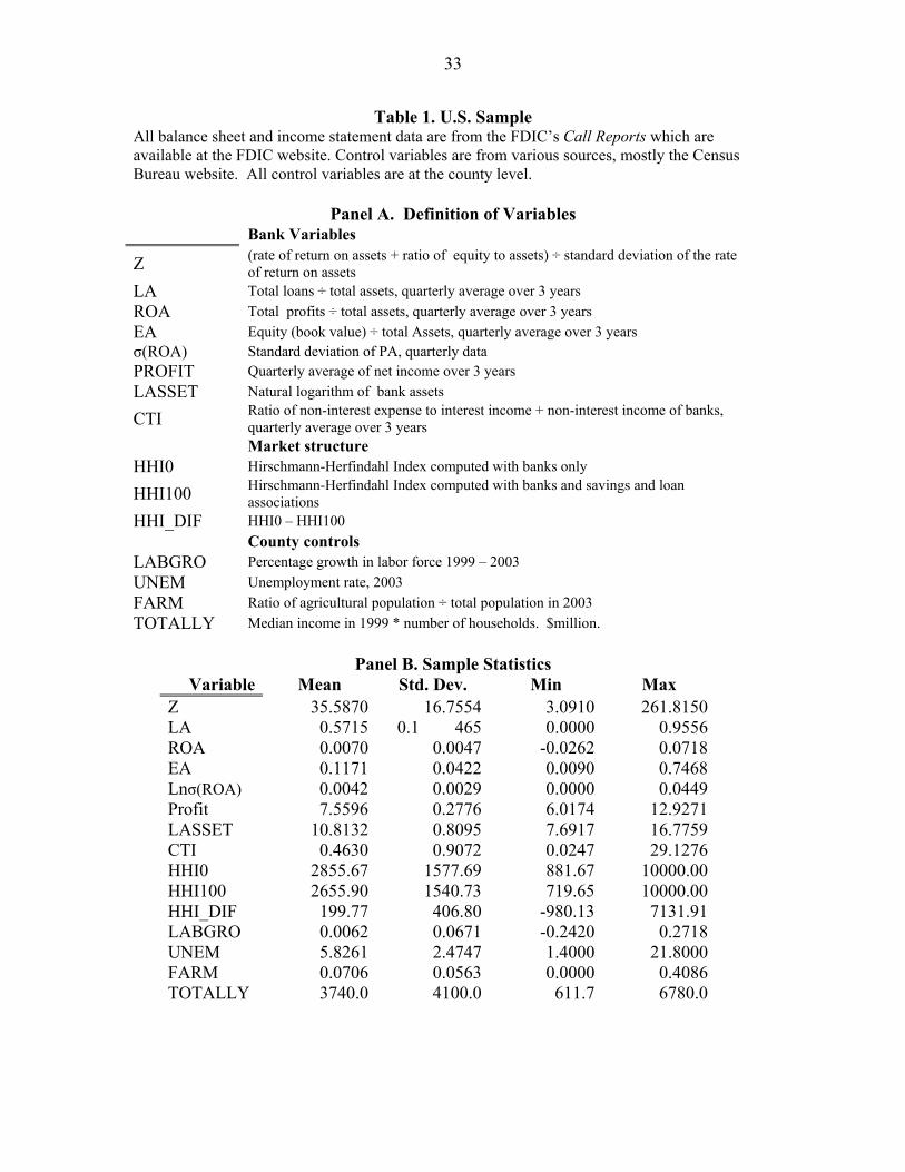
33

Table 1. U.S. Sample All balance sheet and income statement data are from the FDIC’s Call Reports which are available at the FDIC website. Control variables are from various sources, mostly the Census Bureau website. All control variables are at the county level.

Panel A. Definition of Variables

Bank Variables

Z (rate of return on assets + ratio of equity to assets) ÷ standard deviation of the rate of return on assets

LA Total loans ÷ total assets, quarterly average over 3 years ROA Total profits ÷ total assets, quarterly average over 3 years EA Equity (book value) ÷ total Assets, quarterly average over 3 years σ(ROA) Standard deviation of PA, quarterly data PROFIT Quarterly average of net income over 3 years LASSET Natural logarithm of bank assets

CTI Ratio of non-interest expense to interest income + non-interest income of banks, quarterly average over 3 years

Market structure HHI0 Hirschmann-Herfindahl Index computed with banks only

HHI100 Hirschmann-Herfindahl Index computed with banks and savings and loan associations

HHI_DIF HHI0 – HHI100 County controls LABGRO Percentage growth in labor force 1999 – 2003 UNEM Unemployment rate, 2003 FARM Ratio of agricultural population ÷ total population in 2003 TOTALLY Median income in 1999 * number of households. $million.

Panel B. Sample Statistics

Variable Mean Std. Dev. Min Max Z 35.5870 16.7554 3.0910 261.8150 LA 0.5715 0.1 465 0.0000 0.9556 ROA 0.0070 0.0047 -0.0262 0.0718 EA 0.1171 0.0422 0.0090 0.7468 Lnσ(ROA) 0.0042 0.0029 0.0000 0.0449 Profit 7.5596 0.2776 6.0174 12.9271 LASSET 10.8132 0.8095 7.6917 16.7759 CTI 0.4630 0.9072 0.0247 29.1276 HHI0 2855.67 1577.69 881.67 10000.00 HHI100 2655.90 1540.73 719.65 10000.00 HHI_DIF 199.77 406.80 -980.13 7131.91 LABGRO 0.0062 0.0671 -0.2420 0.2718 UNEM 5.8261 2.4747 1.4000 21.8000 FARM 0.0706 0.0563 0.0000 0.4086 TOTALLY 3740.0 4100.0 611.7 6780.0

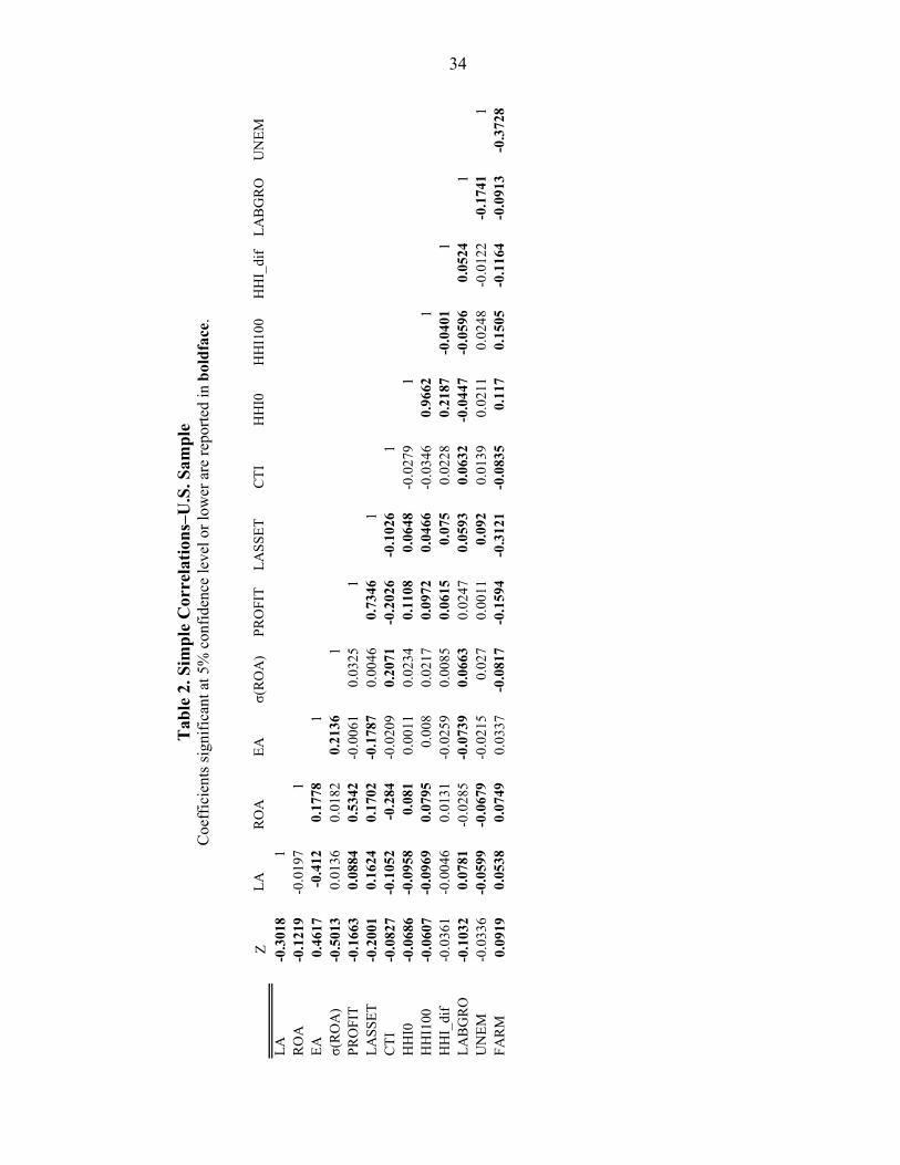
34

T

able

2. S

impl

e C

orre

latio

ns–U

.S. S

ampl

e C

oeff

icie

nts s

igni

fican

t at 5

% c

onfid

ence

leve

l or l

ower

are

repo

rted

in b

oldf

ace.

LAR

OA

EAσ(

RO

A)

PRO

FIT

LASS

ETC

TIH

HI0

HH

I100

HH

I_di

fLA

BG

RO

UN

EMLA

1R

OA

-0.0

197

1EA

-0.4

120.

1778

1σ(

RO

A)

0.01

360.

0182

0.21

361

PRO

FIT

0.08

840.

5342

-0.0

061

0.03

251

LASS

ET0.

1624

0.17

02-0

.178

70.

0046

0.73

461

CTI

-0.1

052

-0.2

84-0

.020

90.

2071

-0.2

026

-0.1

026

1H

HI0

-0.0

958

0.08

10.

0011

0.02

340.

1108

0.06

48-0

.027

91

HH

I100

-0.0

969

0.07

950.

008

0.02

170.

0972

0.04

66-0

.034

60.

9662

1H

HI_

dif

-0.0

046

0.01

31-0

.025

90.

0085

0.06

150.

075

0.02

280.

2187

-0.0

401

1LA

BG

RO

0.07

81-0

.028

5-0

.073

90.

0663

0.02

470.

0593

0.06

32-0

.044

7-0

.059

60.

0524

1U

NEM

-0.0

599

-0.0

679

-0.0

215

0.02

70.

0011

0.09

20.

0139

0.02

110.

0248

-0.0

122

-0.1

741

1FA

RM

0.05

380.

0749

0.03

37-0

.081

7-0

.159

4-0

.312

1-0

.083

50.

117

0.15

05-0

.116

4-0

.091

3-0

.372

8

-0.1

032

-0.0

336

0.09

19

-0.0

827

-0.0

686

-0.0

607

-0.0

361

0.46

17-0

.501

3-0

.166

3-0

.200

1

Z -0.3

018

-0.1

219

35

Table 3. U.S. Regressions: Dependent Variable: Z

Z = (rate of return on assets + ratio of equity to assets) ÷ standard deviation of the rate of return on assets. HHI0 is the Hirschmann-Herfindahl Index computed with banks only. HHI100 is the Hirschmann-Herfindahl Index computed with banks and savings and loan associations. LABGRO is the percentage growth in labor force 1999 – 2003. UNEM is the unemployment rate, 2003. FARM is the ratio agricultural population / total population in 2003. LASSET = natural logarithm of bank assets. CTI = ratio of non-interest expense to interest income + non-interest income of banks, quarterly average over 3 years. TOTALY = median income in 1999 * number of households. Column 3.1 is robust OLS regressions. Column 3.2 is robust OLS regressions with clustering on counties. Column 3.3 is GMM with instrumental variables for HHI0 and LASSET, where the instruments are state dummy variables and HHI_DIF (HHI_DIF = HHI0 – HHI100). See Note.

Equation: 3.1 3.2 3.3

Variable Coeff. t-Stat Coeff. t-Stat Coeff. t-StatConstant 86.1979 ***11.61 86.1979 ***11.43 54.13667 ***4.44 HHI0 -0.0004254 **-1.98 -0.0004254 **-2.0 -0.001221 ***-4.42 TOTALY -9.63E-10 -0.85 -9.63E-10 -0.82 -3.75E-10 -0.56LABGRO -11.75061 **-2.24 -11.75061 **-2.3 -23.91137 ***-5.82UNEM -0.3970404 ***-2.6 -0.3970404 **-2.52 -0.0647434 -0.53FARM 5.495381 0.65 5.495381 0.61 13.39019 *1.7 LASSET -4.271885 ***-6.7 -4.271885 ***-6.55 -1.393676 -1.22CTI -1.853256 ***-3.44 -1.853256 ***-3.37 -1.586964 ***-3.7 R-squared / NOBS 0.0994 2496 0.0994 2496 0.8269 2496 F-test / p-value F(7, 2443) ***14.17 F(7, 2443) ***13.18 RMSE / Categories 16.069 46 16.069 46 16 1280 Hansen J Statistic / Chi-sq p-value ***77.521 0.00135

Regression With: HHI100 -0.0004176 *-1.89 -0.0004176 *-1.92 -0.0016029 ***-3.59

Note: The GMM instrumental variables procedure does not produce a first stage estimate. However, we can do this artificially by separately regressing HHI0, HHI100 and LNASSET on the instruments, which are HHI_DIF and a block of 45 state dummy variables. This produces: HHI0 = 2711.5 + .72 HHI_DIF + State Dummies. Adj R-Sq. = .21, F = 87.0 (84.5) (9.3) (F = 12.0) HHI100 = 2711.4 - .28 HHI_DIF + State Dummies. Adj. R-Sq. = .18, F = 12.9 (84.5) (3.6) (F = 12.0) LASSET = 10.8 + .00009 HHI_DIF + State Dummies. Adj. R-Sq. = .17. (642) (2.3) (f = 12.2)

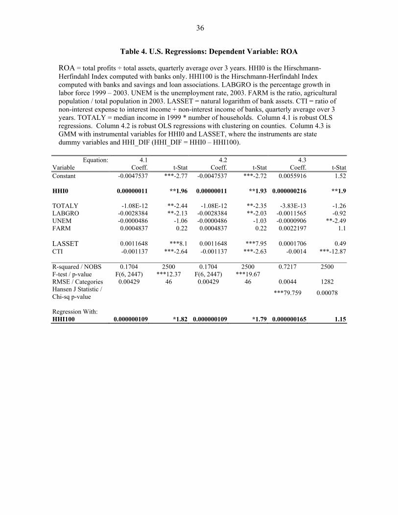
36

Table 4. U.S. Regressions: Dependent Variable: ROA ROA = total profits ÷ total assets, quarterly average over 3 years. HHI0 is the Hirschmann-Herfindahl Index computed with banks only. HHI100 is the Hirschmann-Herfindahl Index computed with banks and savings and loan associations. LABGRO is the percentage growth in labor force 1999 – 2003. UNEM is the unemployment rate, 2003. FARM is the ratio, agricultural population / total population in 2003. LASSET = natural logarithm of bank assets. CTI = ratio of non-interest expense to interest income + non-interest income of banks, quarterly average over 3 years. TOTALY = median income in 1999 * number of households. Column 4.1 is robust OLS regressions. Column 4.2 is robust OLS regressions with clustering on counties. Column 4.3 is GMM with instrumental variables for HHI0 and LASSET, where the instruments are state dummy variables and HHI_DIF (HHI_DIF = HHI0 – HHI100).

Equation: 4.1 4.2 4.3 Variable Coeff. t-Stat Coeff. t-Stat Coeff. t-StatConstant -0.0047537 ***-2.77 -0.0047537 ***-2.72 0.0055916 1.52 HHI0 0.00000011 **1.96 0.00000011 **1.93 0.000000216 **1.9 TOTALY -1.08E-12 **-2.44 -1.08E-12 **-2.35 -3.83E-13 -1.26LABGRO -0.0028384 **-2.13 -0.0028384 **-2.03 -0.0011565 -0.92UNEM -0.0000486 -1.06 -0.0000486 -1.03 -0.0000906 **-2.49FARM 0.0004837 0.22 0.0004837 0.22 0.0022197 1.1 LASSET 0.0011648 ***8.1 0.0011648 ***7.95 0.0001706 0.49CTI -0.001137 ***-2.64 -0.001137 ***-2.63 -0.0014 ***-12.87 R-squared / NOBS 0.1704 2500 0.1704 2500 0.7217 2500 F-test / p-value F(6, 2447) ***12.37 F(6, 2447) ***19.67 RMSE / Categories 0.00429 46 0.00429 46 0.0044 1282 Hansen J Statistic / Chi-sq p-value ***79.759 0.00078

Regression With: HHI100 0.000000109 *1.82 0.000000109 *1.79 0.000000165 1.15

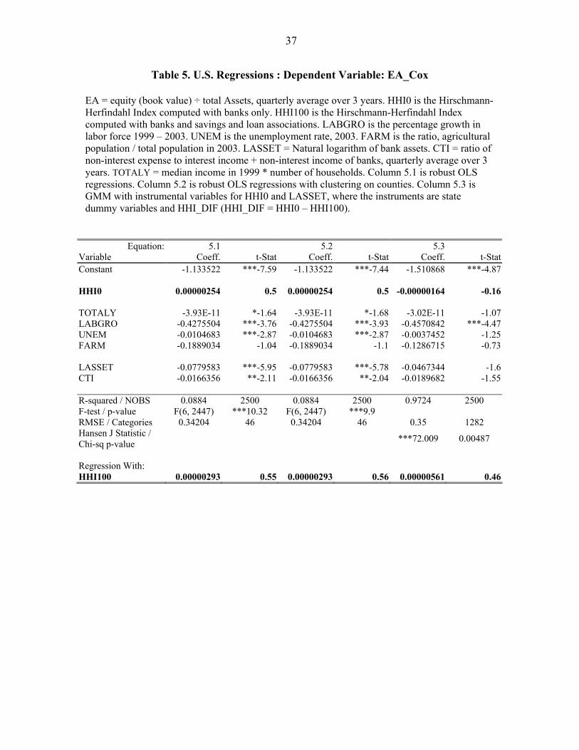
37

Table 5. U.S. Regressions : Dependent Variable: EA_Cox EA = equity (book value) ÷ total Assets, quarterly average over 3 years. HHI0 is the Hirschmann-Herfindahl Index computed with banks only. HHI100 is the Hirschmann-Herfindahl Index computed with banks and savings and loan associations. LABGRO is the percentage growth in labor force 1999 – 2003. UNEM is the unemployment rate, 2003. FARM is the ratio, agricultural population / total population in 2003. LASSET = Natural logarithm of bank assets. CTI = ratio of non-interest expense to interest income + non-interest income of banks, quarterly average over 3 years. TOTALY = median income in 1999 * number of households. Column 5.1 is robust OLS regressions. Column 5.2 is robust OLS regressions with clustering on counties. Column 5.3 is GMM with instrumental variables for HHI0 and LASSET, where the instruments are state dummy variables and HHI_DIF (HHI_DIF = HHI0 – HHI100).

Equation: 5.1 5.2 5.3 Variable Coeff. t-Stat Coeff. t-Stat Coeff. t-StatConstant -1.133522 ***-7.59 -1.133522 ***-7.44 -1.510868 ***-4.87 HHI0 0.00000254 0.5 0.00000254 0.5 -0.00000164 -0.16 TOTALY -3.93E-11 *-1.64 -3.93E-11 *-1.68 -3.02E-11 -1.07LABGRO -0.4275504 ***-3.76 -0.4275504 ***-3.93 -0.4570842 ***-4.47UNEM -0.0104683 ***-2.87 -0.0104683 ***-2.87 -0.0037452 -1.25FARM -0.1889034 -1.04 -0.1889034 -1.1 -0.1286715 -0.73 LASSET -0.0779583 ***-5.95 -0.0779583 ***-5.78 -0.0467344 -1.6CTI -0.0166356 **-2.11 -0.0166356 **-2.04 -0.0189682 -1.55 R-squared / NOBS 0.0884 2500 0.0884 2500 0.9724 2500 F-test / p-value F(6, 2447) ***10.32 F(6, 2447) ***9.9 RMSE / Categories 0.34204 46 0.34204 46 0.35 1282 Hansen J Statistic / Chi-sq p-value ***72.009 0.00487

Regression With: HHI100 0.00000293 0.55 0.00000293 0.56 0.00000561 0.46

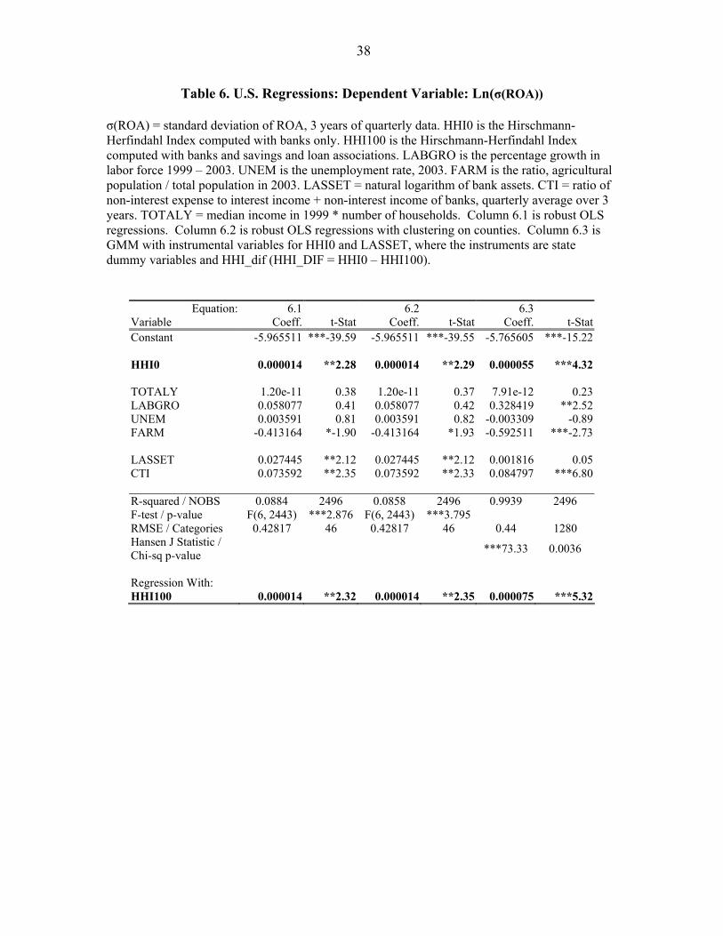
38

Table 6. U.S. Regressions: Dependent Variable: Ln(σ(ROA)) σ(ROA) = standard deviation of ROA, 3 years of quarterly data. HHI0 is the Hirschmann-Herfindahl Index computed with banks only. HHI100 is the Hirschmann-Herfindahl Index computed with banks and savings and loan associations. LABGRO is the percentage growth in labor force 1999 – 2003. UNEM is the unemployment rate, 2003. FARM is the ratio, agricultural population / total population in 2003. LASSET = natural logarithm of bank assets. CTI = ratio of non-interest expense to interest income + non-interest income of banks, quarterly average over 3 years. TOTALY = median income in 1999 * number of households. Column 6.1 is robust OLS regressions. Column 6.2 is robust OLS regressions with clustering on counties. Column 6.3 is GMM with instrumental variables for HHI0 and LASSET, where the instruments are state dummy variables and HHI_dif (HHI_DIF = HHI0 – HHI100).

Equation: 6.1 6.2 6.3 Variable Coeff. t-Stat Coeff. t-Stat Coeff. t-StatConstant -5.965511 ***-39.59 -5.965511 ***-39.55 -5.765605 ***-15.22 HHI0 0.000014 **2.28 0.000014 **2.29 0.000055 ***4.32 TOTALY 1.20e-11 0.38 1.20e-11 0.37 7.91e-12 0.23LABGRO 0.058077 0.41 0.058077 0.42 0.328419 **2.52UNEM 0.003591 0.81 0.003591 0.82 -0.003309 -0.89FARM -0.413164 *-1.90 -0.413164 *1.93 -0.592511 ***-2.73 LASSET 0.027445 **2.12 0.027445 **2.12 0.001816 0.05CTI 0.073592 **2.35 0.073592 **2.33 0.084797 ***6.80 R-squared / NOBS 0.0884 2496 0.0858 2496 0.9939 2496 F-test / p-value F(6, 2443) ***2.876 F(6, 2443) ***3.795 RMSE / Categories 0.42817 46 0.42817 46 0.44 1280 Hansen J Statistic / Chi-sq p-value ***73.33 0.0036

Regression With: HHI100 0.000014 **2.32 0.000014 **2.35 0.000075 ***5.32

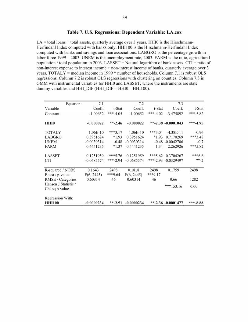
39

Table 7. U.S. Regressions: Dependent Variable: LA.cox

LA = total loans ÷ total assets, quarterly average over 3 years. HHI0 is the Hirschmann-Herfindahl Index computed with banks only. HHI100 is the Hirschmann-Herfindahl Index computed with banks and savings and loan associations. LABGRO is the percentage growth in labor force 1999 – 2003. UNEM is the unemployment rate, 2003. FARM is the ratio, agricultural population / total population in 2003. LASSET = Natural logarithm of bank assets. CTI = ratio of non-interest expense to interest income + non-interest income of banks, quarterly average over 3 years. TOTALY = median income in 1999 * number of households. Column 7.1 is robust OLS regressions. Column 7.2 is robust OLS regressions with clustering on counties. Column 7.3 is GMM with instrumental variables for HHI0 and LASSET, where the instruments are state dummy variables and HHI_DIF (HHI_DIF = HHI0 – HHI100).

Equation: 7.1 7.2 7.3

Variable Coeff. t-Stat Coeff. t-Stat Coeff. t-StatConstant -1.00652 ***-4.05 -1.00652 ***-4.02 -3.475892 ***-5.82 HHI0 -0.000022 **-2.46 -0.000022 **-2.38 -0.0001043 ***-4.95 TOTALY 1.06E-10 ***3.17 1.06E-10 ***3.04 -4.38E-11 -0.96LABGRO 0.3951624 *1.93 0.3951624 *1.93 0.7170269 ***3.48UNEM -0.0030314 -0.48 -0.0030314 -0.48 -0.0042706 -0.7FARM 0.4441235 *1.37 0.4441235 1.34 2.262926 ***5.82 LASSET 0.1251959 ***5.76 0.1251959 ***5.62 0.3704267 ***6.6CTI -0.0685574 ***-2.94 -0.0685574 ***-2.93 -0.0329497 **-2 R-squared / NOBS 0.1643 2498 0.1818 2498 0.1759 2498 F-test / p-value F(6, 2445) ***9.64 F(6, 2445) ***9.17 RMSE / Categories 0.60314 46 0.60314 46 0.66 1282 Hansen J Statistic / Chi-sq p-value ***153.16 0.00

Regression With: HHI100 -0.0000234 **-2.51 -0.0000234 **-2.36 -0.0001477 ***-8.88

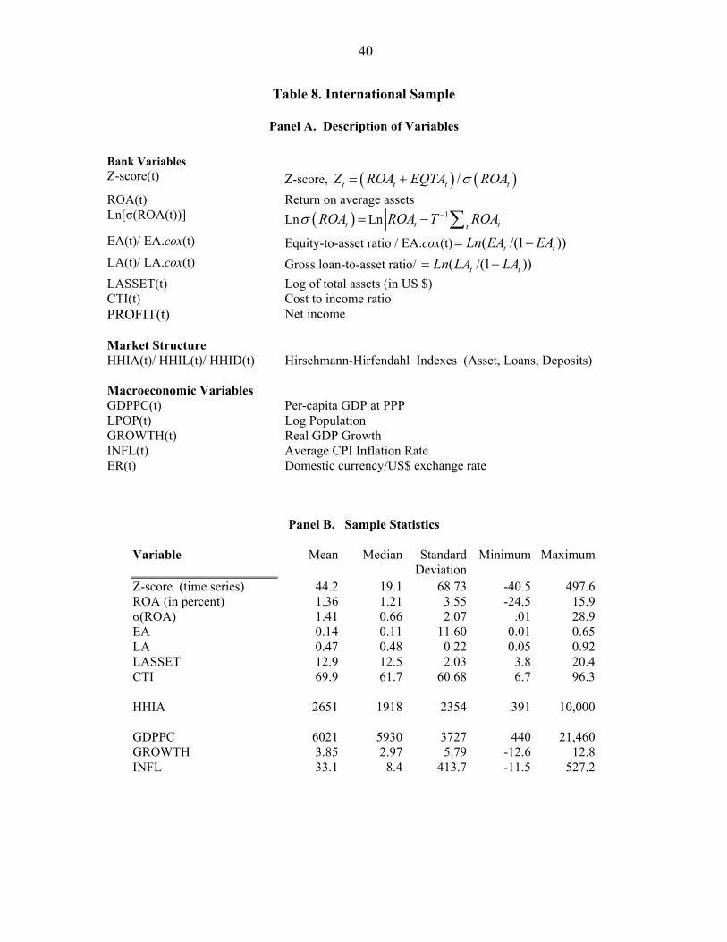
40

Table 8. International Sample

Panel A. Description of Variables

Panel B. Sample Statistics

Variable Mean Median Standard Deviation

Minimum Maximum

Z-score (time series) 44.2 19.1 68.73 -40.5 497.6ROA (in percent) 1.36 1.21 3.55 -24.5 15.9σ(ROA) 1.41 0.66 2.07 .01 28.9EA 0.14 0.11 11.60 0.01 0.65LA 0.47 0.48 0.22 0.05 0.92LASSET 12.9 12.5 2.03 3.8 20.4CTI 69.9 61.7 60.68 6.7 96.3 HHIA 2651 1918 2354 391 10,000 GDPPC 6021 5930 3727 440 21,460GROWTH 3.85 2.97 5.79 -12.6 12.8INFL 33.1 8.4 413.7 -11.5 527.2

Bank Variables Z-score(t) Z-score, ( ) ( )/t t t tZ ROA EQTA ROAσ= + ROA(t) Return on average assets Ln[σ(ROA(t))] Ln ( )tROAσ =Ln 1

t ttROA T ROA−− ∑

EA(t)/ EA.cox(t) Equity-to-asset ratio / EA.cox(t) ( /(1 ))t tLn EA EA= − LA(t)/ LA.cox(t) Gross loan-to-asset ratio/ ( /(1 ))t tLn LA LA= − LASSET(t) Log of total assets (in US $) CTI(t) Cost to income ratio PROFIT(t)

Net income

Market Structure HHIA(t)/ HHIL(t)/ HHID(t) Hirschmann-Hirfendahl Indexes (Asset, Loans, Deposits) Macroeconomic Variables GDPPC(t) Per-capita GDP at PPP LPOP(t) Log Population GROWTH(t) Real GDP Growth INFL(t) Average CPI Inflation Rate ER(t) Domestic currency/US$ exchange rate

41

Tab

le 9

. Cor

rela

tions

–Int

erna

tiona

l Sam

ple

C

oeff

icie

nts s

igni

fican

t at 5

per

cent

con

fiden

ce le

vel o

r low

er a

re re

porte

d in

bol

dfac

e

H

HIA

G

DPP

C

LPO

P G

RO

WTH

IN

FL

Z-sc

ore

(tim

e se

ries)

RO

A

EA

σ(R

OA

) LA

SSET

H

HIA

1.

00

G

DPP

C

-0.3

0 1.

00

LPO

P -0

.25

-0.2

4 1.

00

G

RO

WTH

-0

.01

-0.0

7 0.

07

1.00

IN

FL

0.07

-0

.03

0.05

-0

.08

1.00

Z (ti

me

serie

s)

-0.0

4 0.

02

-0.0

1 0.

08

-0.0

4 1.

00

RO

A

-0.1

4 0.

07

-0.0

2 -0

.08

-0.0

8 0.

07

1.00

EA

0.01

0.

09

-0.0

6 -0

.07

0.01

0.

11

0.16

1.

00

σ(R

OA

) 0.

03

0.03

-0

.01

-0.1

8 0.

01

-0.3

3 -0

.26

0.19

1.

00

LA

SSET

-0

.26

0.27

0.

28

0.07

-0

.01

-0.0

1 -0

.06

-0.4

4 -0

.19

1.00

C

TI

-0.0

3 0.

06

-0.0

2 -0

.04

-0.0

1 -0

.09

-0.4

2 0.

02

0.23

-0

.08

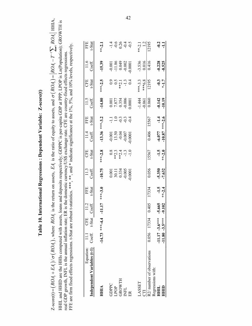
42

Tab

le 1

0. In

tern

atio

nal R

egre

ssio

ns :

Dep

ende

nt V

aria

ble:

Z-s

core

(t)

Z-

scor

e(t)

()

()

/t

tt

ROA

EARO

Aσ

=+

, whe

re

tRO

A is

the

retu

rn o

n as

sets

, t

EA is

the

ratio

of e

quity

to a

sset

s, an

d (

)1

tt

tt

ROA

ROA

TRO

Aσ

−=

−∑

HH

IA,

HH

IL a

nd H

HID

are

the

HH

Is c

ompu

ted

with

ass

ets,

loan

s and

dep

osits

resp

ectiv

ely;

GD

PPC

is p

er-c

apita

GD

P at

PPP

; LPO

P is

Ln(

Popu

latio

n); G

RO

WTH

is

real

GD

P gr

owth

, IN

FL is

the

annu

al in

flatio

n ra

te; E

R is

the

dom

estic

cur

renc

y/U

S$ e

xcha

nge

rate

. CFE

are

cou

ntry

-fix

ed e

ffec

ts re

gres

sion

s.

FFE

are

firm

fixe

d ef

fect

s reg

ress

ions

. t-S

tat a

re ro

bust

t-st

atis

tics.

***,

**,

and

* in

dica

te si

gnifi

canc

e at

the

1%, 5

%, a

nd 1

0% le

vels

, res

pect

ivel

y.

Equa

tion:

11

.1

CFE

11.2

FFE

11.3

CFE

11.4

FF

E11

.5C

FE11

.6FF

EIn

depe

nden

t Var

iabl

es (t

-1)

Coe

ff.

t-Sta

tC

oeff

.t-S

tat

Coe

ff.

t-Sta

tC

oeff

. t-S

tat

Coe

ff.

t-Sta

tC

oeff

.t-S

tat

H

HIA

-1

4.73

***

-4.4

-11.

17**

*-3.

0-1

0.75

***-

2.8

-13.

36 *

**-3

.2-1

4.80

***-

2.5

-15.

39**

-2.1

G

DPP

C

0.

001

0.8

-0.0

01

-1.1

0.00

10.

9-0

.001

-1.4

LPO

P

30.1

1**

2.3

13.5

0 1.

07.

877

0.5

-11.

86-0

.6G

RO

WTH

0.33

4**

2.4

-0.0

4 -0

.30.

354

**2.

10.

049

0.26

INFL

-0.0

05-1

.3-0

.007

-0

.3-0

.006

-1.3

-0.0

02-0

.4ER

-0.0

001

-1.0

-0.0

001

-0.4

0.00

010.

4-0

.000

1-0

.5

LASS

ET

-1.4

44**

*-3.

3-3

.536

**-2

.1C

TI

-0.0

61**

*6.8

0.01

61.

2R

2/ n

umbe

r of o

bser

vatio

ns

0.05

6 17

334

0.40

517

334

0.05

615

567

0.40

6 15

567

0.06

012

195

0.41

612

195

Reg

ress

ions

with

:

H

HIL

-1

1.17

-3.

6***

-5.6

65-1

.5-5

.350

-1.5

-6.0

77

-1.4

-0.1

42-0

.3-0

.228

-0.2

HH

ID

-11.

80 -

3.5*

**-9

.102

**-2

.4-7

.632

**-2

.0-1

0.87

***

-2.6

-10.

19*-

1.7

-8.5

25-1

.1

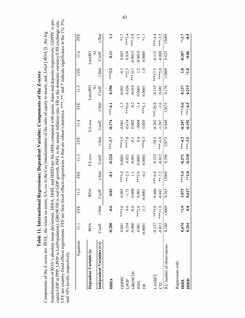
43

Tab

le 1

1. In

tern

atio

nal R

egre

ssio

ns: D

epen

dent

Var

iabl

e: C

ompo

nent

s of t

he Z

-sco

re

Com

pone

nts o

f the

Z-s

core

are

t

ROA

, the

retu

rn o

n as

sets

, EA

.cox

is th

e C

ox tr

ansf

orm

atio

n of

the

ratio

of e

quity

to a

sset

s, an

d (

)(

)t

LnRO

Aσ

, the

log

trans

form

atio

n of

RO

A’s

abs

olut

e m

ean

devi

atio

ns. H

HIA

, HH

IL a

nd H

HID

are

the

HH

Is c

ompu

ted

with

ass

ets,

loan

s and

dep

osits

resp

ectiv

ely;

GD

PPC

is p

er-

capi

ta G

DP

at P

PP; L

POP

is L

n(Po

pula

tion)

; GR

OW

TH is

real

GD

P gr

owth

, IN

FL is

the

annu

al in

flatio

n ra

te; E

R is

the

dom

estic

cur

renc

y/U

S$ e

xcha

nge

rate

. C

FE a

re c

ount

ry-f

ixed

eff

ects

regr

essi

ons.

FFE

are

firm

fixe

d ef

fect

s reg

ress

ions

. t-S

tat a

re ro

bust

t-st

atis

tics.

***,

**,

and

* in

dica

te si

gnifi

canc

e at

the

1%, 5

%,

and

10%

leve

ls, r

espe

ctiv

ely.

Equa

tion:

11

.1

CFE

11.2

FFE

11.3

CFE

11.4

FFE

11.5

CFE

11.6

FFE

Dep

ende

nt V

aria

ble

(t)

RO

A

RO

AEA

.cox

EA.c

oxLn

(σ(R

O A)

Lnσ(

RO A)

Inde

pend

ent V

aria

bles

(t-1

) C

oeff

. t-S

tat

Coe

ff.

t-Sta

tC

oeff

.t-S

tat

Coe

ff.

t-Sta

tC

oeff

.t-S

tat

Coe

ff.

t-Sta

t

H

HIA

-0

.200

-0

.6-0

.03

-0.1

-0.2

24**

*-3.

7-0

.174

***-

4.1

0.39

6**

*3.2

0.11

1.1

GD

PPC

0.

001

***3

.60.

001

***3

.80.

0001

***3

.5-0

.001

-1.5

-0.0

01-0

.30.

002

*1.7

LPO

P 0.

354

0.6

-1.7

1**

-2.3

0.92

1**

*7.0

0.67

4**

*6.6

0.63

6**

2.3

0.93

9**

*3.4

GR

OW

TH

-0.0

06

-0.6

0.00

81.

1-0

.001

-0.5

0.00

20.

2-0

.018

***-

4.7

-0.0

013

***-

3.8

INFL

0.

001

***2

.60.

001

***2

.60.

0001

0.4

-.000

4-1

.40.

0001

1.2

-0.0

019

-1.5

ER

-0.0

001

-1.3

-0.0

001

-0.2

0.00

02**

*4.3

0.00

5**

*4.1

0.00

011.

00.

0005

*1.7

LASS

ET

-0.1

27

***5

.8-0

.466

***-

6.8

-0.2

33-5

4.5

-0.2

02**

*-20

.8-0

.135

***1

7.5

-0.1

15**

*-4.

4C

TI

-0.0

13

***1

1.9

-0.0

41**

-7.2

-0.0

12**

*-6.

9-1

.207

-1.6

0.00

1**

*5.0

-0.0

08**

*-3.

5R

2/ n

umbe

r of o

bser

vatio

ns

0.18

0 13

069

0.56

313

069

0.39

612

673

0.84

812

673

0.17

613

069

0.62

313

069

Reg

ress

ions

with

:

HH

IL

0.67

4 *1

.91.

073

***3

.4-0

.271

***-

4.3

-0.2

47**

*-5.

60.

127

1.0

-0.2

07*-

1.7

HH

ID

0.26

4 0.

80.

617

**2.

0-0

.218

***-

3.5

-0.1

92**

*-4.

50.

215

*1.8

-0.0

6-0

.5

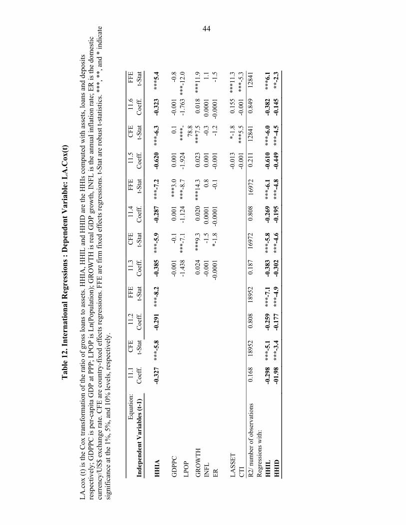
44

Tab

le 1

2. In

tern

atio

nal R

egre

ssio

ns :

Dep

ende

nt V

aria

ble:

LA

.Cox

(t)

LA

.cox

(t) i

s the

Cox

tran

sfor

mat

ion

of th

e ra

tio o

f gro

ss lo

ans t

o as

sets

. HH

IA, H

HIL

and

HH

ID a

re th

e H

HIs

com

pute

d w

ith a

sset

s, lo

ans a

nd d

epos

its

resp

ectiv

ely;

GD

PPC

is p

er-c

apita

GD

P at

PPP

; LPO

P is

Ln(

Popu

latio

n); G

RO

WTH

is re

al G

DP

grow

th, I

NFL

is th

e an

nual

infla

tion

rate

; ER

is th

e do

mes

tic

curr

ency

/US$

exc

hang

e ra

te. C

FE a

re c

ount

ry-f

ixed

eff

ects

regr

essi

ons.

FFE

are

firm

fixe

d ef

fect

s reg

ress

ions

. t-S

tat a

re ro

bust

t-st

atis

tics.

***,

**,

and

* in

dica

te

sign

ifica

nce

at th

e 1%

, 5%

, and

10%

leve

ls, r

espe

ctiv

ely.

Eq

uatio

n:

11.1

C

FE11

.2FF

E11

.3C

FE11

.4

FFE

11.5

CFE

11.6

FFE

Inde

pend

ent V

aria

bles

(t-1

) C

oeff

. t-S

tat

Coe

ff.

t-Sta

tC

oeff

.t-S

tat

Coe

ff.

t-Sta

tC

oeff

.t-S

tat

Coe

ff.

t-Sta

t

HH

IA

-0.3

27

***-

5.8

-0.2

91**

*-8.

2-0

.385

***-

5.9

-0.2

87

***-

7.2

-0.6

20**

*-6.

3-0

.323

***5

.4

GD

PPC

-0.0

01-0

.10.

001

***3

.00.

001

0.1

-0.0

01-0

.8

LPO

P

-1.4

38**

*-7.

1-1

.124

**

*-8.

7-1

.924

****

-78

.8-1

.763

***-

12.0

GR

OW

TH

0.

024

***9

.30.

020

***1

4.3

0.02

3**

*7.5

0.01

8**

*11.

9IN

FL

-0

.001

-1.5

0.00

01

0.8

0.00

1-0

.30.

0001

1.1

ER

-0

.000

1*-

1.8

-0.0

001

-0.1

-0.0

01-1

.2-0

.000

1-1

.5

LASS

ET

-0.0

13*-

1.8

0.15

5**

*11.

3C

TI

-0.0

01**

*5.5

-0.0

01**

*-5.

3R

2/ n

umbe

r of o

bser

vatio

ns

0.16

8 18

952

0.80

818

952

0.18

716

972

0.80

8 16

972

0.21

112

841

0.84

912

841

Reg

ress

ions

with

:

H

HIL

-0

.298

**

*-5.

1-0

.259

***-

7.1

-0.3

83

***-

5.8

-0.2

69

***-

6.1

-0.6

10**

*-6.

0-0

.382

***6

.1H

HID

-0

1.98

**

*-3.

4-0

.177

***-

4.9

-0.3

02**

*-4.

6-0

.195

**

*-4.

8-0

.449

***-

4.5

-0.1

45**

-2.3

45

Table 13. Regressions: Dependent Variable: LPROFIT

Panel A. U.S. Sample

LPROFIT = Ln (PROFIT + A), where A is 1+ the minimum of PROFIT. All regressions include the full set of control variables detailed in Table 3. HHI0 is the Hirschmann-Herfindahl Index computed with banks only. HHI100 is the Hirschmann-Herfindahl Index computed with banks and savings and loan associations. HHI-hat is an instrumental variables estimate of the Hirschman-Herfindahl Index.

Equation: 13.1 13.2 13.3 Variable Coeff. t-Stat Coeff. t-Stat Coeff. t-StatConstant 4.851033 ***32.27 4.851033 ***27.71 5.707693 ***40.86HHI0 5.90E-06 **1.98 5.90E-06 **2.06 HHIhat 8.08E-06 *1.68R-squared / NOBS 0.6211 2500 0.6211 2500 0.9993 2500 F-test / p-value F(6, 2447) ***72.81 F(6, 2447) ***54.93 RMSE / Categories 0.17267 46 0.17267 46 0.19 1282 Hansen J Statistic / Chi-sq p-value ***58.602 0.06931

Regression With: HHI100 6.20E-06 *1.82 6.20E-06 **1.96 5.62E-06 0.99

Panel B. International Sample

LPROFIT = Ln (PROFIT + A), where A is 1+ the minimum of PROFIT. All regressions are with firm fixed effects, and include the full set of control variables detailed in Table 10. HHIA,HHIL and HHID are HHIs computed using total assets, total loans and total deposits respectively.

Equation: 13.4 13.5 13.6

Independent Variables (t-1) #

Coeff. t-Stat Coeff. t-Stat Coeff. t-Stat

HHIA 2.659 **2.07 HHIL 2.711 **2.0 HHID 2.955 *2.22 R2/ number of observations 0.492 13069 0.492 13069 0.491 13069

46

Figure 1. CVH Model (A=0.1, beta=1, r =1.1)

risk shifting parameter

5 10 15 20 25 300

2

4

6

8

10

12profits DEV NMH - MH

5 10 15 20 25 30-2.0

-1.5

-1.0

-0.5

0.0

0.5

1.0profits DEV MH - NMH

5 10 15 20 25 302.25

2.30

2.35

2.40

2.45

2.50

2.55

2.60

2.65

Figure 2. CVH Model (A=0.1, beta=5, r =1.1)

profits DEV NMH - MH

2 4 6 8 10 12 14 16 18 20 22 24 26 28 30-1.00

-0.75

-0.50

-0.25

0.00

0.25

0.50

0.75

1.00profits DEV MH - NMH

2 4 6 8 10 12 14 16 18 20 22 24 26 28 30-0.80

-0.64

-0.48

-0.32

-0.16

0.00

0.16

0.32

Figure 3. BDN Model (A=0.1, alpha=0.5, beta=2, r =1.1)

risk shifting S

10 20 30 40 50 60 70 80 90 100-2

0

2

4

6

8

10loans/deposits

20 40 60 80 100-0.50

-0.25

0.00

0.25

0.50

0.75

1.00

1.25profits/deposits

10 20 30 40 50 60 70 80 90 1000.0

0.1

0.2

0.3

0.4

0.5

0.6

0.7

0.8

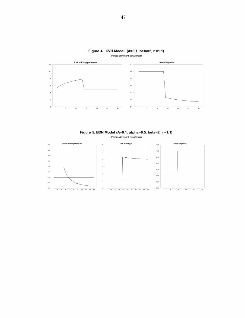
47

Figure 4. CVH Model (A=0.1, beta=5, r =1.1)Pareto dominant equilibrium

Risk shifting parameter

5 10 15 20 25 300

2

4

6

8

10

12Loans/deposits

5 10 15 20 25 300.0

0.2

0.4

0.6

0.8

1.0

1.2

Figure 5. BDN Model (A=0.1, alpha=0.5, beta=2, r =1.1)Pareto-dominant equilibrium

profits NMH/ profits MH

10 20 30 40 50 60 70 80 90 1000.0

0.5

1.0

1.5

2.0

2.5

3.0

3.5

4.0risk shifting S

10 20 30 40 50 60 70 80 90 100-2

0

2

4

6

8

10loans/deposits

20 40 60 80 100-0.50

-0.25

0.00

0.25

0.50

0.75

1.00

1.25

48

References

Allen, Franklin, and Douglas Gale, 2000, Comparing Financial Systems (Cambridge, Massachusetts: MIT Press).

Allen, Franklin, and Douglas Gale, 2004, “Competition and Financial Stability”, Journal

of Money, Credit and Banking, Vol. 36, No. 2, pp. 453-480. Aumann, R, 1959, “Acceptable Points in General Cooperative n-person Games”, in

Contributions to the Theory of Games IV (Princeton, NJ: Princeton University Press).

. Bresnahan, Timothy, 1989, “Empirical Studies of Industries with Market Power,” in

Handbook of Industrial Organization, Vol. II, edited by Schmalensee and Willig (Amsterdam: Elsevier).

Boyd, John H., and Gianni De Nicolò, 2005, “The Theory of Bank Risk Taking and

Competition Revisited,” Journal of Finance, Vol. 60, Issue 3, pp. 1329-343. Boyd, John H. and Edward Prescott, 1986, “Financial Intermediary Coalitions,” Journal

of Economic Theory, Vol. 38, pp. 211-32. De Nicoló, Gianni, 2000, “Size, Charter Value and Risk in Banking: An International

Perspective,” International Finance Discussion Paper No. 689, Board of Governors of the Federal Reserve System.

De Nicolò, Gianni, Phillip Bartholomew, Jhanara Zaman and Mary Zephirin, 2004,

“Bank Consolidation, Internationalization and Conglomeration: Trends and Implications for Financial Risk,” Financial Markets, Institutions & Instruments, Vol. 13, No. 4, pp. 173-217.

Demsetz, Rebecca, and Philip Strahan, 1997, “Diversification, Size, and Risk at Bank

Holding Companies”, Journal of Money, Credit and Banking, Vol. 29, 3, pp. 300-313.

Diamond, Douglas, 1984, “Financial Intermediation and Delegated Monitoring,” Review

of Economic Studies, Vol. 51, pp. 393-414. Hannan, Timothy, 1991, “Foundations of the Structure-Conduct-Performance Paradigm

in Banking,” Journal of Money, Credit and Banking, Vol. 23, No. 1, pp. 68-84. Hellmann, Thomas, Kevin Murdock, and Joseph Stiglitz, 2000, Liberalization, Moral

Hazard in Banking, and Prudential Regulation: Are Capital Requirements Enough?” American Economic Review Vol. 90, No. 1, pp. 147–165.

49

Keeley, Michael, 1990, “Deposit Insurance, Risk and Market Power in Banking,” American Economic Review Vol. 80, 1183–200.

Kreps, David, and Jose Scheinkman, 1983, “Quantity Precommitment and Bertrand

Competition Yield Cournot Outcomes,” Bell Journal of Economics, Vol. 14, pp. 326-37.

Panzar, John, and James Ross, 1971, “Testing for Monopoly Equilibrium,” Journal of

Industrial Economics, Vol. 35, No.4, pp. 443-56. Repullo, Raphael, 2004, “Capital Requirements, Market Power, and Risk-Taking in

Banking,” Journal of Financial Intermediation, Vol. 13, pp. 156-82. Shaffer, Sherrill, 2004, “Comments on What Drives Bank Competition: Some

International Evidence, by Stijn Claessens and Luc Laeven,” Journal of Money, Credit and Banking, Vol. 36, No. 2, pp. 585-92.

Roy, A., 1952, “Safety First and the Holding of Assets,” Econometrica, Vol. 3, No. 20,

pp. 431-49. Williamson, Stephen , 1986, “Costly Monitoring, Financial Intermediation, and

Equilibrium Credit Rationing,” Journal of Monetary Economics, Vol. 18, Issue 2, pp. 159-79.

Wooldridge, Jeffrey, 2003, “Cluster-Sample Methods in Applied Econometrics,”

American Economic Review, Vol. 93, No.2, pp.133-38.