bank holdings and systemic risk celso brunetti, je rey h ... · bank holdings and systemic risk...

Finance and Economics Discussion SeriesDivisions of Research & Statistics and Monetary Affairs

Federal Reserve Board, Washington, D.C.

Bank Holdings and Systemic Risk

Celso Brunetti, Jeffrey H. Harris, and Shawn Mankad

2018-063

Please cite this paper as:Brunetti, Celso, Jeffrey H. Harris, and Shawn Mankad (2018). “Bank Holdings and SystemicRisk,” Finance and Economics Discussion Series 2018-063. Washington: Board of Governorsof the Federal Reserve System, https://doi.org/10.17016/FEDS.2018.063.

NOTE: Staff working papers in the Finance and Economics Discussion Series (FEDS) are preliminarymaterials circulated to stimulate discussion and critical comment. The analysis and conclusions set forthare those of the authors and do not indicate concurrence by other members of the research staff or theBoard of Governors. References in publications to the Finance and Economics Discussion Series (other thanacknowledgement) should be cleared with the author(s) to protect the tentative character of these papers.

Bank Holdings and Systemic Risk

Celso Brunetti◊, Jeffrey H. Harris○ and Shawn Mankad□

Abstract

The recent financial crisis has focused attention on identifying and measuring systemic

risk. In this paper, we propose a novel approach to estimate the portfolio composition of

banks as function of daily interbank trades and stock returns. While banks’ assets are

reported to regulators and/or the public at relatively low frequencies (e.g. quarterly or

annually), our approach estimates bank asset holdings at higher frequencies allowing us

to derive precise estimates of (i) portfolio concentration within each bank (a measure of

diversification) and (ii) common holdings across banks (a measure of market

susceptibility to propagating shocks). We find evidence that systemic risk measures

derived from our approach lead, in a forecasting sense, several commonly used systemic

risk indicators.

Key words: Bank holdings, concentration index, similarity index, systemic risk

JEL: G21, C11, G11

◊Federal Reserve Board ([email protected]); ○American University

([email protected]); □ Cornell University ([email protected]) corresponding author, this material is based upon work supported by the National Science Foundation under Grant No. 1633158 (Mankad).

We would like to thank seminar participants in the Cornell University OTIM seminar series, the 2018 IAQF-Thalesians seminar series at NYU, the 10th International Conference of the ERCIM WG on Computational and Methodological Statistics, London 2017, and the U.S. Securities and Exchange Commission for comments and suggestions.

The views in this paper should not be interpreted as reflecting the views of the Board of Governors of the Federal Reserve System or of any other person associated with the Federal Reserve System. All errors and omissions, if any, are the authors’ sole responsibility.

1

1 Introduction

The 2007-09 financial crisis accentuated the need for effective monitoring,

oversight and regulation of complex financial institutions which trade thousands

of financial products in markets around the world. This paper presents a method

for estimating individual bank holdings and systemic risk in the banking system

in between periodic financial reports, providing a more timely and on-going

assessment of individual bank diversification and systemic risk. Our practical

method draws upon two informationally-linked data sources available at the daily

frequency: (i) stock returns and (ii) interbank lending activity. Stock returns are

of course widely and publicly available, while interbank lending data is accessible

to central banks.

We build on the accounting framework of Shin (2009, 2010) starting with

annual reports, and use stock returns and interbank lending data to extract daily

estimates of the assets held by individual banks. 1 We then estimate the

composition of each individual bank’s underlying (unobserved) portfolio each

month and show that our methods provide meaningful and timely information

about both individual bank holdings and systemic risk in the banking system.

Our methods involve solving a matrix factorization problem within a novel

Bayesian estimation framework (details in Section 2 below). First, we estimate

each individual bank’s underlying asset portfolio which we then use to

1 See also Elliott et al. (2014) and Brunetti et al. (forthcoming). We partition yearly balance sheets of the banking sector to isolate the underlying (and unobserved) portfolios held by banks. This partitioning, when combined with balance sheet identities, implies a variant of the non-negative matrix factorization problem (extensively studied in other domains, e.g. Lee and Seung, 1999). In particular, our matrix factorization problem requires solving for one factor that is subject to probability constraints.

2

characterize risk within and among banks. Intuitively, we derive an index of

portfolio concentration (bank-specific risk) for each individual bank and an index

of portfolio similarity across banks (systemic risk) which captures market

susceptibility to propagating shocks to any asset class.

The concentration of assets in an individual bank’s portfolio has well-known

risk implications (Klein and Bawa, 1977; Santis and Gerard, 1997; Gale and

Gottardi, 2017; Pastor, Stambaugh and Taylor, 2017). By estimating the monthly

asset holdings, our methods allow regulators to better assess, in a timely manner,

concentrated risk within a bank without having to directly examine bank balance

sheets. Moreover, the similarity of bank portfolios indicates interconnectedness,

an important measure for the propagation of shocks (see e.g. Greenwood et al.,

2015, Caccioli et al., 2014, 2015).

While our methods indirectly estimate bank holdings, we demonstrate that

these estimates closely approximate real balance sheet data. We validate our

estimates rigorously in two ways. First, since the statistical model and estimation

framework are novel, we produce Monte Carlo simulations to demonstrate that

our estimation approach produces reliable results. With these simulations we

compare different estimation techniques to demonstrate that our Bayesian

approach is the most reliable. Second, we validate the model from an accounting

point of view by showing that our progressive monthly estimates closely match

real accounting data year over year.

Once we estimate the asset composition of each bank portfolio, we derive

bank sector indices of concentration across individual portfolios and common

holdings across different banks. Both indices convey important information in a

3

forecasting sense—a more concentrated and similar banking sector is a leading

factor and harbinger of market stress at monthly horizons. In this respect, our

paper contributes to a growing literature on measures of systemic risk, where

scholars have created various other risk indices.2

Our measures differ from what the literature has proposed thus far.

Alternative risk measures primarily relate to capital adequacy and hence are

more concerned with the liability side of bank balance sheets, while our measures

focus on the asset side of the balance sheet. Our concentration measure captures

bank portfolio concentration specific to a bank risk profile, and our measure of

common holdings links the riskiness of each bank to other banks in the system. A

shock to an undiversified bank could have a larger impact on the bank’s balance

sheet and can more readily propagate to other banks which hold similar portfolios.

With these differences in mind, we also examine our systemic risk

indicators relative to alternative risk measures including three measures of

systemic risk published by the ECB, several macro indicators, Acharya et al.’s

(2017) MES and Brownlees and Engle’s (2017) SRISK. Our concentration index

(one-way) Granger-causes MES and SRISK, suggesting that information from

stock returns and interbank trading feeding into the asset side of bank balance

sheets emerges prior to information from the liability side.

2 Various other systemic risk measures have been proposed (see Biasis, Flood, Lo and Valavanis (2012) for a survey). Acharya, Pedersen, Philippon and Richardson (2017) estimate MES based on the (expected) amount a bank is undercapitalized in a crisis event. Brownlees and Engle (2017) measure SRISK as the contribution of each firm in terms of capital shortfall in severe market movements. Adrian and Brunnermeier (2016) compute CoVaR, the value at risk (VaR) for the financial sector conditional on a bank having had a VaR loss. Huang, Zhou and Zhu (2009) combine CDS default probabilities of individual banks and forecasted asset return correlations. Giudici, Sarlin and Spelta (forthcoming), combine direct exposures with common exposures—i.e. what Brunetti et al. (forthcoming) refer to as correlation and physical networks. See also Segoviano and Goodhart (2009), de Jonghe (2010) and Tarashev, Borio and Tsasaronis (2010).

4

Additionally, we show that the higher moments of our measures (standard

deviation, skewness and kurtosis) also convey information. The standard

deviation and skewness of our measures generally lead (one-way Granger-cause)

measures of systemic risk published by the ECB—the Composite Systemic Risk

Index, the Simultaneous Default Probability, and the Sovereign Composite

Systemic Risk Index—as well as EU macroeconomic indicators such as the

Consumer Confidence Index (CCI), the Purchasing Managers' Index (PMI) and

Retail Sales.

Our approach provides a novel method for regulators to monitor the

banking sector. Using daily interbank lending and stock market returns

aggregated each month,3 our method provides insight into the balance sheets of

banks at a higher frequency than the more cumbersome and less timely quarterly

or annual disclosures or audits allow. Moreover, our methods complement other

approaches to assess and monitor systemic risk that build on network science

techniques (Billio et al., 2012; Diebold and Yılmaz, 2014; Brunetti et al.,

forthcoming; Giudici et al., forthcoming). Our derivations and methodology also

provide a blueprint for how entity-level information from multiple markets can be

combined in a principled manner using matrix factorization and balance sheet

models to improve the quality of subsequent risk and interconnectedness

measures.

3Our procedure is flexible. While we employ daily data on stocks and interbank activity to derive monthly measures of bank holdings, bank holdings can be computed at any frequency beyond one day. More generally, our procedure estimates bank holdings at any frequency lower than the input data, so for example, intraday data allows for daily bank holding estimates.

5

Our method is also practical, drawing on the vast and increasing amounts

of data generated by new regulatory frameworks—e.g. the Dodd-Frank Wall

Street Reform and Consumer Protection Act (Dodd-Frank), European Banking

Authority, European Securities and Markets Authority, and the Financial

Stability Board. Dodd-Frank, for instance, requires exchanges and market

participants to record and report data to regulators. Despite these increased

reporting requirements, most regulators can only access data directly related to

their legal purview, so that integrating data from myriad products across various

regulated and unregulated markets remains a significant challenge. Our method

provides practical means for assessing complex financial institutions which trade

hundreds of financial products in markets around the world. Of course, other

applications remain beyond the scope of this current work and we leave the

process of combining data across markets to further research efforts.

2 An Accounting Framework

As a starting point for building our systemic risk measures, we first employ the

accounting framework as in Shin (2009, 2010), Elliott et al. (2014) and Brunetti

et al. (forthcoming) wherein individual bank balance sheets are connected via

interbank lending and common holdings, and then aggregated to the industry

level. Let there be n banks under consideration and X be the vector of interbank

debt (the total value of liabilities held by other banks). Π is the share of bank i’s

liabilities held by bank j, W is the weight invested in each of the K assets by bank

i ∑ 1 , Y denotes the market value of bank i’s assets, e indicates bank

i’s equity (which we proxy for with the market value of equity), and d is the total

value of liabilities of bank i held by non-banks.

6

Consider a financial system in which banks connect lenders to borrowers as

intermediaries, collecting deposits from households and firms and investing the

deposits in a portfolio of assets, including loans to the household sector (via

mortgages and consumer debt) and firms. The balance sheet for any individual

bank i can be partitioned as follows.

Assets Liabilities

ei

xi

Π di

We obtain the balance sheet identity as

Π

or, using matrix notation, as

ΠΧ ⨀

where u is a vector of ones of length K; ⨀ denotes the Schur product (element wise

multiplication), so that ⨀ and . We can therefore express the

portfolio of assets held by each bank as follows

⨀ Π

where I is the n × n identity matrix.

Recall that D represents debt claims on the banking sector by households,

mutual and pension funds and other non-bank institutions. Following Shin (2009),

we assume that the debt liabilities to non-banks evolve slowly. We also assume

that W, the weight invested in each of the K assets, evolves slowly, whereas the

7

value of the corresponding asset holdings fluctuates more rapidly over time (e.g.

from day to day, or week to week). Thus, over appropriately short intervals,

changes to D and to W are negligible; then changes in the balance sheet from

period t-1 to t can be written as

⨀ Π Π

⨀ Π Π . (1)

We assume that changes to the equity account can be readily measured

for public banks from public stock prices, wherein the market incorporates

important information about the bank into daily stock prices. In this light, stock

returns reflect information about the assets and liabilities on the bank’s balance

sheet.

Additionally, daily transaction-level interbank lending data can be used to

construct a daily estimate of Π , the adjacency matrix of interbank transactions,

and X , the vector of debt held by other banks. Note that X can only be partially

observed—banks can lend each other money through other (often unobservable)

mechanisms. For instance, the European banks which we study can trade across

the e-MID electronic system (which we observe and utilize), bilaterally in the over-

the-counter (OTC) market, or with the ECB directly. Despite this fact, our

factorization method is able to produce robust estimates of W, the vector of weights

each bank invests in each asset, which we utilize to construct our systemic indices.

8

3 Balance Sheet Driven Bayesian Factorization

Given the accounting identity that links banks together through interbank

lending arrangements and common asset holdings, we aim to quantify the

portfolio composition of each bank. Using our notation from above, let

Π Π

and

.

Written in element form, Equation (1) implies that the i-th bank’s balance sheet

satisfies

∑ .

Assuming that the investment opportunity set is the same for all banks, we can

express the same equation in matrix form

(2)

subject to ∑ 1 for all and 0 for all , , where , , … , is

an n T matrix, W is an n K matrix with non-negativity constraints on the rows,

and , , … , is an K T matrix.4

Equation (2) can be readily seen as a variant of the non-negative matrix

factorization (NMF) problem, where Z is given and the objective is to estimate W

and V. Most works in NMF do not include the sum to one constraint for

computational reasons, which results in an identifiability problem. Specifically,

the estimates in NMF are always re-scalable (so-called scale invariance), where

W can be multiplied by a positive constant c and V by 1/c to obtain different W, V

4 Non-negativity implies no short selling, which we believe is reasonable, given regulatory restrictions on bank portfolios and the intermediary role that banks play in the economy.

9

without changing their product. In other words, under conventional NMF

formulations, it is not possible to differentiate between a change in the percentage

asset class holding and the change in value of the given asset class. We note that

in our case this identifiability issue is resolved, since we require that the rows of

W to sum to one.5 However, due to the sum-to-one constraint in addition to the

non-negativity on W, the resultant problem is challenging to solve.6

In this light, we develop a novel Bayesian estimation framework, capturing

the non-negativity and probability constraints using appropriate distributional

assumptions.7 Specifically, we assume that each row of W, denoted by , is

distributed according to a Dirichlet distribution with common concentration

parameter α.

Dirichlet (3)

The Dirichlet distribution, whose range is all discrete probability distributions of

length K, is commonly utilized in nonparametric Bayesian statistics to model

unknown probability distributions (Antoniak, 1974, Sethuraman, 1994).8 is the

common parameter, which can take any value greater than zero. As gets larger,

5We note that our proposed factorization model is not fully identifiable, as the columns of W (and correspondingly in V) are subject to permutation and can thus be arbitrarily ordered. This is a common property of most factorization models other than the Singular Value Decomposition.6 The main contributions in non-negative matrix factorization typically pose an optimization problem based on minimizing the Frobenius norm of the difference between Z and the estimated factors to obtain an estimate of W and V in (2) (Lee and Seung, 1999, Lin, 2007, Mankad et al., forthcoming). When faced with sum-to-one constraints, the usual approach is to find approximate solutions (i.e., continuous relaxation of constraint via a LaGrangian penalty) or to ignore the constraint in the estimation and normalize the factors ex-post in a second stage (see, e.g., Huck et al. (2010) and Heinz et al. (2001)). Both have computational advantages, but do not guarantee robust solutions. Indeed, we find that conventional optimization methods can provide qualitatively different solutions depending on the random seed, reducing the practical application of these methods. 7 This contrasts with previous Bayesian factorization models that have a similar framework but solve for non-negativity without the probability constraint (Schmidt et al., 2009, Psorakis et al., 2011). 8 More recently, it has been popularized in the Latent Dirichlet Allocation model of Blei et al. (2003) and applied extensively for summarizing unstructured text data with so-called topic modeling analysis. We use this distribution for the rows of W to capture the probability constraint.

10

the probabilities are closer to uniform, meaning that the assets held within each

bank portfolio and across banks are approximately equal. As approaches zero,

the distribution is sparser (more weights are zero, though the zero components

can vary among banks).

Since represents changes in asset values at the daily level, over long

enough intervals we expect its distribution be unimodal and centered on a small

constant capturing market trends. We also expect the true distribution of to

have heavier tails as has been established for stock returns (Upton and Shannon,

1979), but we show the Gaussian distribution offers a suitable approximation with

computational advantages. As such, elements of V are assumed to be

independently normally distributed with mean µ and variance

∏ ,, . (4)

Note that, while the prior distribution assumes that the daily returns between

asset classes are independent, the posterior distribution of V will in general

exhibit correlations between asset classes. 9 Thus, in effect, the correlation

structure between asset returns is learned implicitly through the estimation we

describe in this section below.

We introduce one last random variable, , that controls the variance of

additive Gaussian noise on each element of the matrix Z and is modeled with an

inverse gamma density with shape and scale θ.10

, (5)

9 See the last sub-section of Appendix 1 for mathematical details. 10 The inverse gamma density as a prior distribution for the noise variance σ2 is a natural choice and extensively utilized by Brav (2000), Cremers (2002), Jones (2003), and Korteweg and Sorensen (2010).

11

To complete the Bayesian specification, we assume that Z has the following

conditional likelihood

| , , ∏ , . (6)

Equations (2) and (6) can be viewed as mixture models, where Gaussian

means encoded within the columns of are added together using weights in .11

The number of components in the mixture are determined by the rank of the

factors and , which is set by the analyst. With such mixture models, others

have shown that with enough components the resultant mixture distribution

given by has sufficient flexibility to approximate any continuous distribution

for (subject to regularity conditions) to an arbitrary degree of accuracy (see

Norets and Pelenis, (2012) and Rossi (2014)).12 This also provides intuition for

when our model will not work well. We expect our Bayesian specification to

struggle if the true distribution of is discontinuous, truncated, or having other

boundary effects. In our data, we see no evidence for this concern.

We briefly discuss estimation of the Bayesian model next, with full

derivations provided in the Appendix. By Bayes rule, the joint posterior is

proportional to

p W, V, σ |Z ∝ p Z|W, V, p W p V p , (7)

where we utilize the fact that , , and are assumed to be independently

distributed as in Equations (3)-(6).

11 We use the normal distribution again for tractability and ease of computation, though this does not necessarily sacrifice the overall accuracy of the factorization even when Z follows a non-Gaussian distribution. 12 The intuition for this result is that any density can be well approximated using multiple small variance normal components with different means to position the components appropriately.

12

Computing the posteriors densities p W|Z and p V|Z requires solving an

intractable integral of the joint posterior distribution in Equation (7). To overcome

this challenge, we utilize a combination of standard Markov Chain Monte Carlo

(MCMC) methods. The basic idea behind MCMC is to construct a Markov chain

that has the desired distribution as its limiting distribution. Thus, once the

Markov chain has converged to its equilibrium, repeatedly sampling states of the

chain provides an empirical estimate of the desired distribution that is accurate

to an arbitrarily high degree. From this empirical distribution, the expectation can

be readily calculated.13

Since we can apply conjugate distributional properties14 to derive explicit,

closed forms of the posterior distributions for and conditional on the data ( )

and the current state of each of the parameters ( , , ), we use Gibbs sampling

to estimate the marginal distributions | and | . In other words, the

Markov chain is defined by the conditional posterior distributions and iterated

until convergence as in any MCMC method, after which samples are drawn and

averaged to derive point estimates.

We use a more general version of Gibbs Sampling, the Metropolis Hastings

algorithm, to estimate | , because the conditional posterior distribution of

is not composed of conjugate distributions and thus cannot be characterized

analytically. The estimation procedure exploits the fact that we are still able to

13 See Casella and George (1992) and Chib and Greenberg (1995) for further information on MCMC methods, including best practices and how to determine whether the Markov chain has converged to its limiting distribution. 14 In Bayesian probability theory, if the posterior distributions (e.g., p V│Z ) are in the same family as the prior probability distribution (e.g., p(V)), the prior and posterior are conjugate distributions which have a closed-form expression for the posterior distribution.

13

compute the value of a function (shown explicitly in the Appendix) that is

proportional to the desired distribution. This proportion is used to generate

Markovian samples iteratively that converge to the desired distribution as the

number of samples grows.

4 Validating the Model

In this section, we validate our model and Bayesian estimation framework from

both a statistical perspective through a simulation exercise, and from an

accounting perspective by comparing the estimates of W (the vector of weights

invested in each asset class) against actual balance sheet data reported annually

by each bank. In both tasks, we first utilize non-parametric hypothesis tests to

compare the distribution of the true W with its estimate. Specifically, we utilize

four well known non-parametric tests. The Brown-Mood median test (Brown et

al., 1951) and the Fisher-Pitman permutation test (Boik, 1987) assess whether

two samples have identical medians and means, respectively. The third test is the

more general Mann-Whitney U test (Mann and Whitney, 1947) which compares

the full distributions of the estimated and true W to assess whether our estimate

is stochastically smaller (or larger) than its true value. 15 And lastly we utilize the

Two Sample Anderson Darling Test (Scholz and Stephens, 1987 following

Anderson and Darling, 1954) to assess whether there are differences between the

two samples with particular sensitivity at the tails of the distributions.16

15 To understand the precise hypothesis tested by the Mann-Whitney U test, let x and y be two random variables with cumulative distribution functions f and g respectively. The hypotheses for the test : ∙ ∙ versus : , ∀ . 16 This is comparable to the Kolmogorov-Smirnov test, which is not as appropriate in our setting since the real balance sheet data has multiple zero values. Moreover, the Anderson Darling test has been shown in Monte-Carlo studies to have comparatively greater statistical power (Razali et al., 2011).

14

Note that element-wise accuracy comparisons for (like mean squared

errors) are not possible given the large number of asset classes and that the

columns of the estimated can be ordered arbitrarily, a common property of such

factorization models. As such, in addition to the four distributional tests, we also

report the Rand Index, a classic accuracy measure for this setting (Rand 1971).

The Rand Index varies from zero to one, with larger values indicating more

accurate estimates. Lastly, to understand the accuracy of the overall factorization

we report a Pseudo R2, which is analogous to the R2 in linear regression.17

Additionally, we compare the accuracy of our proposed model relative to

competing optimizing techniques (from the matrix factorization and machine

learning literature) that can be used to solve Equation (2). The methods we

compare against are as follows:

1. The Semi Non-Negative Matrix Factorization model of Ding et al. (2010)

with probability constraints enforced ex-post, which is state of the art in

the matrix factorization field;

2. Fuzzy K-means, a classic machine learning algorithm, that produces

estimates of based on a Gaussian mixture model (Bezdek et al., 1984).

4.1 Simulation

We test the accuracy and validity of the proposed model under different simulation

settings. The first simulation establishes self-consistency of the proposed

factorization, that is, we generate the matrix Z from the model implied by the

factorization. Then we perform the estimation with perfect knowledge of the true

17 The PseudoR2 1‖ ̅‖

.

15

underlying parameterizations. In practice, this information would not be known

at the start of the estimation, but we need to establish the validity of the

estimation procedure. The second simulation misspecifies the hyper-parameters

and initial values to help us gain insight into the sensitivity and validity of our

estimation under the more realistic condition that the underlying

parameterizations are unknown.

First, we generate W, V, and σ according to their distributions, where the

concentration value and initializations are set to be equal to the values used in

our real data—i.e. balance sheet data from annual reports. We use 0.2, 0,

0.45, 100, and 0.5 with W and V of dimension 49 × 8 and 8 × 23,

respectively, also chosen to match the real data. 18 Second, under the hyper-

parameter misspecification scenario, we perform the estimation with the value of

the prior parameter α ranging from 0.15 to 0.35 (the true value always remains

0.20). Studying the performance of the estimation for varying levels of α

misspecification is particularly important, as α is also the main parameter for the

distribution of . For completeness we also incorrectly initialize 1, ,

1 and 1, so that every hyper-parameter is misspecified.

Panel A in Table 1 presents the results of the self-consistency scenario.

Each of our four non-parametric statistical tests indicate that the model and

estimation is self-consistent. Note that the average p-values shown in parentheses

in Table 1 are above 5% for all tests, so in this setting, we fail to reject the null

18 The number of banks in our sample is not fixed since during our sample period there have been mergers, acquisitions and bankruptcies. The choice of 49 banks in the simulation is only indicative of the number of banks in our sample. Bank identities in the interbank market are confidential. The number of investment assets, 8, is the result of the banks’ balance sheet analysis. Details are discussed in the data section.

16

hypotheses from each of the four tests. The pseudo R2 and Rand Index also provide

evidence that the estimation overall and of specifically are high quality, with

values close to one. Thus, our estimates of W, which are particularly important

within the systemic risk context, match well the true distribution when using the

ex-post correct parameterization.

Panel B in Table 1 presents results for values of α ranging from 0.15 to 0.35

(straddling the actual 0.2 value) in various hyper-parameter misspecification

scenarios. The pseudo R2 values show that the overall quality of the estimation

remains high and is essentially unaffected by misspecified hyper-parameters,

which is perhaps expected given that in Bayesian analysis the posterior

distribution uses the observed data to recalibrate prior assumptions. Focusing on

, for all α, our tests largely show that the estimated and true distributions are

statistically identical (except under the most conservative Anderson-Darling test).

We regard this as evidence that our estimation procedure is robust to mild

misspecification. In fact, while the Rand Index decreases when the hyper-

parameters are misspecified, the performance under misspecification is still

superior to competing methods (as shown in Panel C). Given the numerical

evidence that the estimation is statistically valid and performs favorably with

alternative techniques, we now turn our attention to whether the model can be

validated in terms of actual balance sheet data.

4.2 Validation with Balance Sheet Data

To estimate Wat the monthly frequency, we aggregate daily interbank trading

data coupled with aggregated daily stock returns of publicly-traded European

17

banks spanning January 2006 through December 2012.19 We obtain interbank

trading data from e-MID,20 the only electronic market for interbank deposits in

the Euro region, which offers interbank loans ranging from overnight (one day) to

two years in duration, with overnight contracts representing 90% of total volume

during our sample period (see Brunetti et al. (2011)). Our e-MID trading data

includes a large number of banks, but we analyze only those which are publicly-

traded. We integrate the e-MID data through the balance sheet, coupling assets

traded overnight with the corresponding daily stock returns which proxy for

equity changes. The number of publicly-traded banks in our data ranges between

45 and 60 and span several European countries. Our sample includes large,

medium and small size banks, but for confidentiality reasons we do not identify

specific banks. Summary statistics for the publicly-traded banks in our sample are

shown in Table 2, where we see that their average daily interest rate in the e-MID

dropped post-Lehman (starting September 12, 2008), while daily volume started

to decline much earlier when the ECB noted worldwide liquidity shortages

(August 7, 2007). Daily volume for the publicly-traded banks declined from over 1

billion euros prior to the start of the financial crisis to 100 million euros post-

Lehman. As the crises unfolded, the banks experienced negative stock returns

with increasing volatility.

We assume that banks rebalance their overall portfolios monthly, so we

estimate W each month using the Bayesian framework.21 Recall, however, that

19 We stop in December 2012 because liquidity in the e-MID market largely dried up as shown in Brunetti et al. (forthcoming). 20 E-MID data can be purchased at: https://www.e-mid.it/en/e-services/data-service/ 21 When beginning the MCMC estimation each month, W, V, and are initialized to their estimates from the previous month. 20,000 samples are drawn using a burn-in of 10,000 iterations.

18

, … is constructed with daily stock returns and daily e-MID activity as

proxies for equity changes and interbank activity, respectively.

Using public data from annual reports, we construct the true vector of

weights held across eight investment types, W, by first partitioning the balance

sheets of each bank on December 31 each year into eight categories: Cash,

Commercial Loans, Intangible Assets, Interbank Assets, Residential Loans,

Investments, Other Holdings, and Remainder (total assets minus all other

categories).22 Then we arrange the balance sheet into a matrix, with each row as

a bank, i.e., W is a N × 8 matrix, where N is the number of banks in our sample.

Lastly, we normalize W, by dividing each entry by its row sum (each bank’s total

assets). Importantly, in the validation exercise as well as in our estimates, the

number of asset categories we consider varies from 4 to 8. Our results are robust

to the choice of the number of asset categories.23

We compare the density of our estimated as of December 31 of each year

in our sample to the observed W constructed using real balance sheet data,24 see

Figure 1. Note that our estimates closely approximate actual values except for the

tails of the distribution—in the actual data approximately 44 percent of values

are less than 1% (i.e. an individual bank holds a very small amount of a particular

asset), while in our estimated , 44 percent of values are less than 4%. We show

in the next section that this difference is not practically meaningful, but it does

22To further improve the results, asset categories can be made to be more granular. There is a trade-off however, since as the number of asset categories increases, the estimation procedure becomes more cumbersome because the number of parameters increases dramatically. 23 Additional results available upon request. 24 We performed a grid search to find the best value according to the log-likelihood of the final factorization on the observed data. This was done both every month and once simultaneously for all time points. Results were qualitatively similar between both approaches.

19

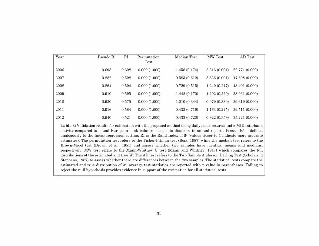
affect the non-parametric statistical tests as reported in Table 3. We consistently

fail to reject the null hypothesis for the permutation test (same mean) and median

test (same median). Interestingly, the Mann-Whitney U test, which compares the

full distributions of the estimated and true W, indicates that at the onset of the

crisis, 2006-2008, the estimates of W are statistically different from the true data

but during and after the crisis, 2009-2012, our procedure produces significantly

more accurate estimates of the distribution of W. This is confirmed by the pseudo

R2 which indicates that our factorization explains more variation in Z during and

after the crisis.

The Anderson-Darling test rejects the null due to the differences on the

lower tail highlighted above. Consistent with these hypothesis tests, the pseudo

R2 and Rand Index show that the estimation quality is generally good, with values

clearly bounded away from zero.25 More generally, these results resemble the

misspecification scenario in the simulation study, where the Anderson-Darling

test is rejected but all other metrics indicate accurate estimates. Overall, we

believe that the bulk of this evidence supports that our estimates of W are accurate

and drawn from nearly identical distributions to the true W.

4.3 The Source of Information: Stock Returns versus Interbank Trades

In this sub-section we examine the importance of each information source (daily

stock returns versus interbank lending activity) on the final estimate of W. We

repeat the validation procedure above by estimating W using only daily stock

25 Tables A1 and A2 in the Appendix show results for estimation under competing methods. The competing approaches tend to achieve slightly higher Rand Index values, but massively underperform with the hypothesis testing compared to our proposed approach.

20

returns (omitting interbank lending information) and separately by using only

daily e-MID interbank lending activity (omitting stock returns).

Tables 4 and 5 show the results of the non-parametric statistical tests that

compare the two sets of estimates to the true balance sheet weights held by banks

in our sample across the eight investment types. We highlight two main patterns

in the results. First, the pseudo R2 values show that the factorization model

explains much less variation when using only stock return data (Table 4), whereas

the quality of the estimates is generally better when considering the e-MID data

only (Table 5). Second, while the two estimates of W do share distributional

similarities with the true balance sheet data, we see that for several sample years

we reject the null hypothesis for the Median test and Mann-Whitney U tests and

both sets of estimates continue to fail the Anderson-Darling test, due to differences

in the tails of the distributions.

Not surprisingly, we find that the results from estimating W using both

data sources (Table 3) are stronger compared to estimation results using

individual data sources. Moreover, while both the interbank market and the stock

market convey information (albeit differently), the interbank market data maps

more directly to bank assets. Importantly however, these sources can be combined

with our methods to obtain more precise estimates of bank holdings and therefore

more precise estimates of bank-specific and systemic risk.

5. Compiling Systemic Risk Measures

Having established the validity of our approach in estimating portfolio weights

across the spectrum of the banks in our sample, we now turn our attention to two

key questions: i) Are bank portfolios well-diversified? ii) How similar are portfolio

21

holdings across banks? To answer the first question we develop a concentration

index which captures the degree of diversification of each bank’s portfolio. To

answer the second question, we develop a similarity index which captures how

similar portfolio holdings are across banks. We view these two metrics as

indicators of systemic risk within the banking system. First, concentrated

holdings on a small number of assets within an individual bank exposes the bank

to asset-specific risk. Ceteris paribus, should a bank with a portfolio concentrated

only in one or two assets be forced to sell those assets—the price impact of these

actions could be higher when compared to a bank liquidating a more diversified

portfolio. This measure of risk is specific to the bank.

Second, the similarity of asset holdings across banks suggests that shocks

to any particular asset class will be borne across the entire banking system. The

similarity of portfolio holdings is the theoretical justification of network analysis

such as Diebold and Yilmaz (2014) and Billio et al. (2012), and is based on a simple

consideration: if two banks, A and B, hold the same asset, and an exogenous shock

forces A to liquidate the asset, the price of the asset will decline and therefore

change the value of B’s portfolio potentially leading to B also selling the asset at

an unfavorable price. Braverman and Minca (2014) adopt this argument to

describe how common asset holdings can transmit financial distress among

banks.26 Our similarity measure captures the network effect in that is describing

a propagation mechanism. In case of a shock to a bank, the concentration measure

26 Others have obtained similar theoretical findings establishing that overlapping portfolios and common assets holdings can serve to amplify economic shocks, thus raising the chances of simultaneous failures (Wagner, 2010; Beale et al., 2011; Haldane and May, 2011; Raestin, 2014; Caccioli et al., 2014, 2015; Greenwood et al., 2015).

22

tells us how risky a bank’s portfolio is while the similarity measure assesses the

likelihood that the shock will propagate. Note that an advantage of our approach

is to allow estimation of portfolio weights at a higher frequency than typically

reported in official bank filings.

After obtaining an estimate for W in a given month, we calculate a

Herfindahl index (Rhoades, 1993) of diversification/concentration across our eight

asset categories. Specifically, let the superscript (t) index time in months, then

∑ . (8)

To measure the similarity in assets held across banks, we define the pairwise

portfolio similarity between bank i and bank j as

∑ , . (9)

The similarity27 index is bounded between 0 and 1, with zero values indicating

each pair of banks hold different assets while values equal to one indicating both

banks hold identical asset portfolios. For example, assume two banks and three

assets and the following holdings:

Bank A Bank B Similarity Index Component

Investment 1 50% 30% 30%



27 In unreported results, we measure similarity using the Euclidean distance, KL divergence, correlation, and cosine similarity (as in Getmansky et al. (2017) for the insurance industry) and several other criteria. Results are consistent across these different similarity measures.

23

The example shows that the index has the desirable property of been bounded

between zero (no common holdings) and 1 (same holdings and same and weights),

and captures portfolio similarities adequately. However, it may underestimate

contagion since, if Bank A is hit by a shock and liquidates most if its assets, the

value of the entire B’s portfolio will be affected.28

Within the banking system, asset concentration and portfolio similarity are

related. If an individual bank holds a concentration of assets that perform poorly

ex-post, the poor performance might stress other institutions. Likewise, if each

bank in the system is fully diversified across asset classes, then, by definition, all

bank balance sheets will be similar and highly interconnected. In this regard, we

posit that the interdependence between asset concentration and bank similarity

reflects systemic risk.

Figure 2 displays the first four cross-sectional moments of the Herfindahl

distribution of bank asset concentration/diversification over time. As the figure

shows, European banks grew more concentrated (on average) from 2006 through

September 2008 when Lehman Brothers failed. During the following year,

however, the average concentration fell dramatically before gradually rising again

to near pre-Lehman levels through 2012. The standard deviation of asset

concentration has risen alongside the rise in concentration since mid-2009.

Notably, the skewness and kurtosis of asset concentration was falling pre-

Lehman, but rose dramatically in the subsequent four months, suggesting that

individual bank holdings were less concentrated and banks were investing in

28 The similarity index could be modified to account for regulatory standards. For example, we could give more weight to asset classes based on liquidity characteristics.

24

different portfolios. Both skewness and kurtosis of asset concentration remained

high through mid-2011 before falling dramatically through 2012.

Figure 3 displays the first four moments of pairwise portfolio similarity over

time. The average similarity among European banks generally rose from 2008

through mid-2010 before falling through 2012. Overall, the standard deviation of

similarity increased from 2006-2008 and remained relatively high through 2012.

The skewness of similarity is negative and, after becoming more negative from

2008-2010, has reverted toward zero through 2012. The kurtosis of similarity

appears to follow the opposite pattern from skewness. While the patterns in

moments of asset concentration and portfolio similarity suggest that these metrics

may reflect real economic conditions, we aim to test whether these metrics are

useful for forecasting purposes.

5.1 Comparison with ECB risk and macro indicators

Recall that our monthly metrics are constructed using daily interbank trades and

daily equity price changes, so that we impound both expected future performance

as well as current liquidity demands for each bank. As a benchmark test for the

usefulness of these metrics in forecasting, we relate moments of concentration and

similarity to three measures of systemic risk published by the ECB—the

Composite Systemic Risk Index, the Simultaneous Default Probability, and the

Sovereign Composite Systemic Risk Index. The Composite Systemic Risk

Indicator is a weighted average of several measures of financial stress that focus

on different aspects of the financial system including money, bond, equity and

forex markets as well as financial intermediaries. The Simultaneous Default

25

Probability, and the Sovereign Composite Systemic Risk Index are essentially

CDS implied probabilities.29

Figure 4 displays these three ECB metrics from 2006 through 2012.30 Note

that the ECB metrics all rise from early 2007 through early 2009 before abating

slightly until early 2010. All three metrics then rise through late 2011 before

generally falling off through 2012. These metrics have been extensively used—e.g.

Hollo et al (2012).

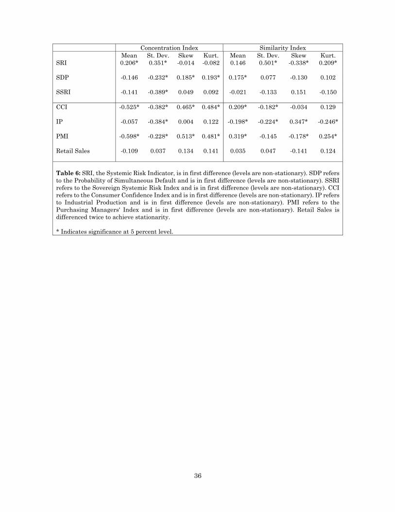
Table 6 reports the contemporaneous correlation between the moments of

our concentration and similarity indices and the three measures of systemic risk

published by the ECB—these measures are in first difference to guarantee

stationarity.31

Interestingly, the higher is the concentration in the banking sector (mean),

the higher is the Composite Systemic Risk Index (SRI), which captures stress

conditions in European markets. Similarly, higher levels of variation (standard

deviation) in concentration and similarities across bank portfolios are associated

to higher levels of stress conditions. The systemic risk indicator is also linked to

higher moments of the similarity index. The Probability of Simultaneous Default

is positively correlated to the similarity index indicating that when the similarity

index is high, the probability of default is increasing (recall that the ECB systemic

indicators are in first difference and hence they indicate a change). Overall, we

29 ECB Financial Stability Review, June 2012, p.99 available at: https://www.ecb.europa.eu/pub/pdf/other/financialstabilityreview201206en.pdf?6b3b7eb08f53f6ad069f5b6dd15275c8 30 The Simultaneous Default Probability metric is only available since 2007. 31 We perform two stationarity tests, the generalized least squares Dickey–Fuller (DF) test proposed by Elliott, Rothenberg, and Stock (1996) and the Augmented Dickey-Fuller (ADF) test.

26

find strong contemporaneous linkages between the ECB systemic risk measures

and our indices.

The second part of Table 6 reports contemporaneous correlations between

major EU macroeconomic indicators—the Consumer Confidence Index (CCI),

Industrial Production (IP), the Purchasing Managers' Index (PMI) and Retail

Sales—and the moments of the concentration and the similarity indices (also in

this case, all variables have been differenced to accommodate for non-

stationarity). Table 6 indicates strong contemporaneous linkages between macro

variables and our indices. Recall that our indices are computed using data on the

interbank market, e-MID, which is capturing interbank activities only in part, and

stock market returns of a relatively small number of publicly traded banks.

Nevertheless, the correlation between our indices and macro variables is

statistically significant.

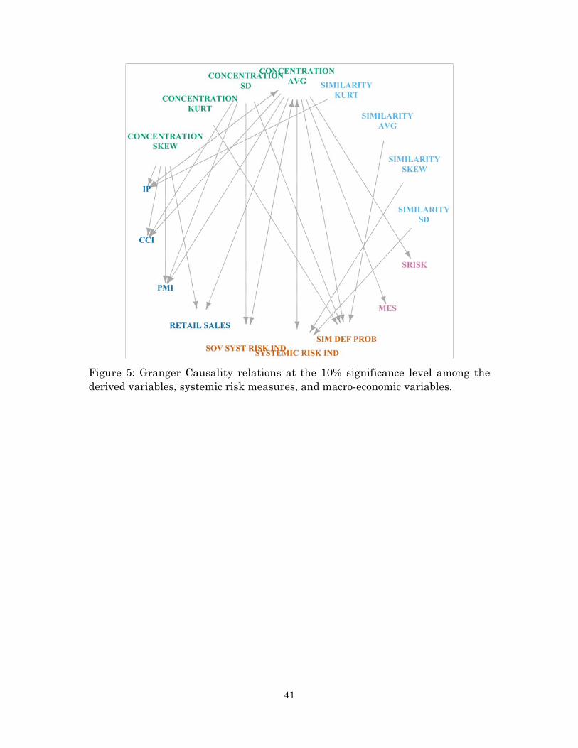
We further investigate the lead-lag relations among the moments of our

indices and the ECB systemic risk and macro indicators by estimating bivariate

VARs and testing for Granger-non-causality.32 Figure 5 presents the results of our

analysis. → indicates that A Granger-causes B at the 10 percent significance

level, while ↔ indicates feedback effect, i.e. A Granger-causes B and B

Granger-causes Aat the 10 percent significance level. Figure 5 shows that, with

only a few exceptions of feedback effects, our indices are able to cause, in a

forecasting sense, most of the ECB systemic risk and macro indicators.

Interestingly, the first three moments of the concentration index seem to contain

valuable information for forecasting.

32 VARs optimal lag specification is based on AIC. Standard errors are bootstrapped.

27

5.2 Comparison with MES and SRISK

Acharya et al (2017) develops a model of systemic risk in which the level of

capitalization of the financial sector has implication on the real economy. In the

model, the contribution of each financial institution to systemic risk is measured

by the systemic expected shortfall, a function of how much the institution is

undercapitalized conditional on the entire financial system being

undercapitalized. The systemic expected shortfall depends on the institution’s

leverage and on the institution’s marginal expected shortfall (MES). Acharya et

al (2017) show that MES is able to predict systemic risk in the recent financial

crisis.

Brownlees and Engle (2017) introduce a conditional capital shortfall

measure of systemic risk, named SRISK. This measure captures the contribution

of a financial institution to systemic risk and, similar to Acharya et al (2017), is

based on the capital shortfall of the institution conditional on a severe market

downturn. SRISK is able to capture the riskiness of US financial institutions

leading to the 2007-2009 crisis. Aggregating SRISK across institutions, the

authors also propose an early warning index of distress.

Both MES and SRISK combine balance sheet information and asset price

information for publicly traded financial institutions. We took both measures and

compared them to our indices.33 The measures were provided to us on a company-

by-company basis. We selected all European companies in the countries where the

33 We are thankful to Rob Capellini, director of the V-Lab at NYU, for sharing the data. Source: The Volatility Laboratory of the NYU Stern Volatility Institute (https://vlab.stern.nyu.edu)

28

e-MID banks are based.34 In total we construct MES and SRISK measure using

313 financial institutions including banks, insurance companies, broker/dealers.

To aggregate MES and SRISK measures across institutions, we normalize these

measures by market capitalization. Note that our concentration and similarity

indices are computed by examining 45-60 banks while MES and SRISK have been

computed over a much larger set of institutions.

Figure 6 depicts MES and SRISK together with the concentration index and

the similarity index over time. MES, SRISK and our concentration index exhibit

similar patterns after the crisis. In fact, the correlation coefficients between the

concentration index and MES and SRISK are 43% and 39%, respectively.

However, our similarity index evolves much differently than MES, SRISK and

concentration, suggesting that our method uncovers two distinct sources of

systemic risk—individual bank concentration and common holdings across banks.

We further investigate the lead-lag relationships among MES, SRISK,

concentration and similarity through the lens of bivariate VARs and Granger-

causality tests. We find that the concentration index leads, in a forecasting sense,

both the MES (p-value = 0.073) and SRISK (p-value = 0.076). The reverse is not

true—i.e. SRISK and MES do not Granger-cause the concentration index. As

suggested by patterns in Figure 6, we do not find any Granger-causality between

the similarity index and either MES or SRISK. These results suggest that

information about bank assets (via interbank loans and equity returns) emerges

34 For confidentiality reasons we cannot match the two datasets exactly — i.e., we cannot select the companies in V-Lab with the banks in our e-MID dataset.

29

prior to information from bank liabilities (which largely underlie MES and

SRISK), a finding relevant to regulators charged with bank oversight.

6 Conclusion

In this paper, we propose a novel approach to estimate the monthly portfolio

composition of banks as a function of daily interbank trades and stock returns. We

start our estimation with the balance sheets (reported annually) for 50-60

publicly-traded European banks at the beginning of January 2006, compiling

precise estimates of portfolio concentration within each bank and common

holdings across banks. We consider portfolio concentration as a measure of bank

diversification and common holdings as a measure of market susceptibility to

propagating shocks.

From this starting point, we estimate the evolution of monthly bank asset

holdings using daily interbank trades and equity price changes in a stylized

representation of aggregate industry balance sheets. We validate our findings

using simulation methods and benchmarking our estimates from year to year

(when new balance sheet data becomes available). Our tests demonstrate that

information from daily interbank and equity markets are useful for tracking the

evolution of bank asset holdings over time.

We use these more frequent and timely holdings estimates to construct two

systemic risk measures--individual bank portfolio concentration and common

holdings across banks. We find evidence that these systemic risk measures lead,

in a forecasting sense, several other commonly used systemic risk indicators,

suggesting that our method provides a robust forecasting tool for market

regulators to assess systemic risk in a timely manner. Moreover, while our model

30

estimates bank asset holdings at higher frequencies than available from annual

or quarterly reports, our method can be readily applied to other situations where

higher frequency market data might provide valuable information to regulators

between formal audits or other regulatory reports.

31

Panel A: Self-Consistency Scenario

Pseudo R2 RI Permutation Test Median Test MW Test AD Test

0.20 0.936 0.824 0.000 (1.000) -1.147 (0.369) 0.323 (0.682) 2.249 (0.091)

Panel B: Hyper-Parameter Misspecification Scenario

Pseudo R2 RI Permutation Test Median Test MW Test AD Test

0.10 0.929 0.757 0.000 (1.000) 0.247 (0.610) 0.862 (0.425) 4.698 (0.009)

0.15 0.938 0.762 0.000 (1.000) 0.428 (0.587) 1.049 (0.352) 4.362 (0.041)

0.20 0.938 0.776 0.000 (1.000) 0.566 (0.595) 1.272 (0.256) 3.332 (0.045)

0.25 0.936 0.775 0.000 (1.000) 0.761 (0.518) 1.576 (0.148) 6.939 (0.005)

0.30 0.941 0.782 0.000 (1.000) 0.609 (0.521) 1.711 (0.119) 9.212 (0.001)

Panel C: Competing Methods

Method Pseudo R2 RI Permutation Test Median Test MW Test AD Test

Semi-NMF 0.800 0.740 0.000 (1.000) 0.623 (0.587) -0.135 (0.779) 4.248 (0.015)

Fuzzy K-Means NA 0.633 0.000 (1.000) 4.112 (0.004) 3.078 (0.010) 106.406 (0.000)

Table 1: Simulation results averaged over 100 iterations. Pseudo R2 is defined analogously to the linear regression setting; RI is the Rand Index of (values closer to 1 indicate more accurate estimates). The permutation test refers to the Fisher-Pitman test (Boik, 1987) while the median test refers to the Brown-Mood test (Brown et al., 1951) and assess whether two samples have identical means and medians, respectively. MW test refers to the Mann-Whitney U test (Mann and Whitney, 1947) which compares the full distributions of the estimated and true W. The AD test refers to the Two Sample Anderson Darling Test (Scholz and Stephens, 1987) to assess whether there are differences between the two samples. The statistical tests compare the estimated and true distribution of ; average test statistics are reported with p-value in parentheses. Failing to reject the null hypothesis provides evidence in support of the estimation for all statistical tests. Note that Pseudo R2 is not reported for the Fuzzy K-Means algorithm, because it only estimates and an estimate of both and is required.

32

Pre-Crisis Jan 1 2006 – Aug 7 2007

Crisis 1 Aug 8 2007 – Sept 12 2008

Mean St. Dev. Skew Kurt. Mean St. Dev. Skew Kurt. Stock Returns 0.001 0.141 1.070 507.643 -0.001 0.155 0.904 506.349 Volume (e-MID) 1637.923 1204.923 1.039 0.541 553.403 562.621 2.054 5.243 Rate (e-MID) 3.185 0.566 -0.039 -1.325 4.026 0.191 -0.597 1.719 Crisis 2

Sept 16 – Apr 1 2009 Crisis 3

Apr 2 2009 – Dec 31 2012 Mean St. Dev. Skew Kurt. Mean St. Dev. Skew Kurt. Stock Returns -0.005 0.194 1.932 431.219 -0.002 0.200 0.211 560.613 Volume (e-MID) 158.231 103.638 1.152 0.658 158.333 158.640 1.232 -0.299 Rate (e-MID) 2.837 1.313 -0.190 -1.488 0.783 0.286 0.219 -1.913 Table 2: Summary statistics at the daily level for log stock returns, e-MID trading volume (millions of Euros), and e-MID interest rate. All e-MID statistics are computed using transactions that include at least one of the banks in our sample as a counter-party in the overnight loan.

33

Year Pseudo R2 RI Permutation Test

Median Test MW Test AD Test

2006 0.698 0.698 0.000 (1.000) 1.458 (0.174) 3.316 (0.001) 22.771 (0.000)

2007 0.882 0.598 0.000 (1.000) 0.583 (0.612) 3.326 (0.001) 47.608 (0.000)

2008 0.864 0.594 0.000 (1.000) -0.729 (0.515) 1.249 (0.217) 48.401 (0.000)

2009 0.910 0.595 0.000 (1.000) -1.442 (0.170) 1.202 (0.229) 38.931 (0.000)

2010 0.930 0.575 0.000 (1.000) -1.010 (0.344) 0.979 (0.330) 39.619 (0.000)

2011 0.916 0.584 0.000 (1.000) 0.433 (0.719) 1.163 (0.245) 39.511 (0.000)

2012 0.940 0.521 0.000 (1.000) 0.433 (0.720) 0.922 (0.359) 35.221 (0.000)

Table 3: Validation results for estimation with the proposed method using daily stock returns and e-MID interbank activity compared to actual European bank balance sheet data disclosed in annual reports. Pseudo R2 is defined analogously to the linear regression setting; RI is the Rand Index of (values closer to 1 indicate more accurate estimates). The permutation test refers to the Fisher-Pitman test (Boik, 1987) while the median test refers to the Brown-Mood test (Brown et al., 1951) and assess whether two samples have identical means and medians, respectively. MW test refers to the Mann-Whitney U test (Mann and Whitney, 1947) which compares the full distributions of the estimated and true W. The AD test refers to the Two Sample Anderson Darling Test (Scholz and Stephens, 1987) to assess whether there are differences between the two samples. The statistical tests compare the estimated and true distribution of ; average test statistics are reported with p-value in parentheses. Failing to reject the null hypothesis provides evidence in support of the estimation for all statistical tests.

34



2006 0.027 0.603 0.000 (1.000) 2.663 (0.011) 1.356 (0.177) 1.498 (0.077)

3.376 (0.014)

1.506 (0.086)

8.956 (0.000)

22.46 (0.000)

0.314 (0.256)

4.356 (0.006)

2007 0.061 0.563 0.000 (1.000) 2.364 (0.022) 1.634 (0.103)

2008 0.012 0.514 0.000 (1.000) 1.440 (0.175) 0.847 (0.401)

2009 0.009 0.733 0.000 (1.000) -4.873 (0.000) -3.202 (0.001)

2010 0.047 0.505 0.000 (1.000) -7.987 (0.000) -4.675 (0.000)

2011 0.001 0.583 0.000 (1.000) 0.000 (1.000) -0.730 (0.467)

2012 0.001 0.568 0.000 (1.000) -1.717 (0.101) -1.968 (0.049)

Table 4: Validation results for estimation using the proposed model estimated using only daily stock returns data compared to actual European bank balance sheet data disclosed in annual reports. Pseudo R2 is defined analogously to the linear regression setting; RI is the Rand Index of (values closer to 1 indicate more accurate estimates). The statistical tests compare the estimated and true distribution of ; test statistics are reported with the p-value in parentheses. Failing to reject the null hypothesis provides evidence in support of the estimation for all statistical tests.

35



2006 0.878 0.518 0.000 (1.000) 2.291 (0.028) 1.000 (0.317) 2.793 (0.024)

7.613 (0.000)

4.349 (0.000)

5.473 (0.002)

6.264 (0.001)

7.701 (0.000)

3.373 (0.010)

2007 0.841 0.498 0.000 (1.000) 3.644 (0.000) 1.795 (0.073)

2008 0.787 0.439 0.000 (1.000) 2.332 (0.023) 1.178 (0.237)

2009 0.893 0.418 0.000 (1.000) 1.010 (0.346) 0.621 (0.533)

2010 0.886 0.401 0.000 (1.000) 1.587 (0.130) 0.777 (0.436)

2011 0.911 0.467 0.000 (1.000) 1.442 (0.168) 0.707 (0.478)

2012 0.897 0.480 0.000 (1.000) 1.010 (0.348) 0.776 (0.438)

Table 5: Validation results for estimation using the proposed model estimated using only daily e-MID data compared to actual European bank balance sheet data disclosed in annual reports. Pseudo R2 is defined analogously to the linear regression setting; RI is the Rand Index of (values closer to 1 indicate more accurate estimates). The statistical tests compare the estimated and true distribution of ; test statistics are reported with the p-value in parentheses. Failing to reject the null hypothesis provides evidence in support of the estimation for all statistical tests.

36

Concentration Index Similarity Index Mean St. Dev. Skew Kurt. Mean St. Dev. Skew Kurt. SRI 0.206* 0.351* -0.014 -0.082 0.146 0.501* -0.338* 0.209* SDP -0.146 -0.232* 0.185* 0.193* 0.175* 0.077 -0.130 0.102 SSRI -0.141 -0.389* 0.049 0.092 -0.021 -0.133 0.151 -0.150 CCI -0.525* -0.382* 0.465* 0.484* 0.209* -0.182* -0.034 0.129 IP -0.057 -0.384* 0.004 0.122 -0.198* -0.224* 0.347* -0.246* PMI -0.598* -0.228* 0.513* 0.481* 0.319* -0.145 -0.178* 0.254* Retail Sales -0.109 0.037 0.134 0.141 0.035 0.047 -0.141 0.124 Table 6: SRI, the Systemic Risk Indicator, is in first difference (levels are non-stationary). SDP refers to the Probability of Simultaneous Default and is in first difference (levels are non-stationary). SSRI refers to the Sovereign Systemic Risk Index and is in first difference (levels are non-stationary). CCI refers to the Consumer Confidence Index and is in first difference (levels are non-stationary). IP refers to Industrial Production and is in first difference (levels are non-stationary). PMI refers to the Purchasing Managers' Index and is in first difference (levels are non-stationary). Retail Sales is differenced twice to achieve stationarity. * Indicates significance at 5 percent level.

37

Figure 1: Distribution of the observed elements in aggregated from all available years compared to the estimated W aggregated over the same times.

38

Figure 2: Concentration index summary statistics over time. The vertical lines denote three events: 1) August 7, 2007 when the ECB noted worldwide liquidity shortages; 2) September 12, 2008 (Lehman default); 3) April 1, 2009 when the ECB announced the end of the recession.

39

Figure 3: Similarity index summary statistics over time. The vertical lines denote three events: 1) August 7, 2007 when the ECB noted worldwide liquidity shortages; 2) September 12, 2008 (Lehman default); 3) April 1, 2009 when the ECB announced the end of the recession.

40

Figure 4: Time series of systemic risk measures published by the ECB (Systemic Risk Indicator, Simultaneous Default Probability, and Sovereign Systemic Risk Indicator – source ECB). The vertical lines denote three events: 1) August 7, 2007 when the ECB noted worldwide liquidity shortages; 2) September 12, 2008 (Lehman default); 3) April 1, 2009 when the ECB announced the end of the recession.

41

Figure 5: Granger Causality relations at the 10% significance level among the derived variables, systemic risk measures, and macro-economic variables.

42

Figure 6: MES and SRISK indices and Concentration and Similarity indices. The vertical lines denote three events: 1) August 7, 2007 when the ECB noted worldwide liquidity shortages; 2) September 12, 2008 (Lehman default); 3) April 1, 2009 when the ECB announced the end of the recession.

MES and SRISK, Source: The Volatility Laboratory of the NYU Stern Volatility Institute (https://vlab.stern.nyu.edu).

43

References

Acharya, V. V., L. H. Pedersen, T. Philippon and M. Richardson. Measuring systemic risk. Review of Financial Studies, 30(1), 2–47, 2017.

Adrian, T. and M. K. Brunnermeier. CoVar. American Economic Review, 106(7), 1705-1741, 2016.

Anderson, T. W. and D. A. Darling. A test of goodness of fit. Journal of the American statistical association, 49(268):765–769, 1954.

Antoniak, C. E. Mixtures of Dirichlet processes with applications to Bayesian nonparametric problems. The Annals of Statistics, pages 1152–1174, 1974.

Bezdek, J. C., R. Ehrlich, and W. Full. Fcm: The fuzzy c-means clustering algorithm. Computers & Geosciences 10(2-3), 191-203, 1984.

Biasis, D., M. D. Flood, A.W. Lo and S. Valavanis. A survey of systemic risk analytics. Annual Review of Financial Economics, 4, 255-296, 2012.

Billio, M., M. Getmansky, A. W. Lo, and L. Pelizzon. Econometric measures of connectedness and systemic risk in the finance and insurance sectors. Journal of Financial Economics, 104(3):535–559, 2012.

Blei, D. M., A. Y. Ng, and M. I. Jordan. Latent Dirichlet allocation. Journal of Machine Learning Research, 3(Jan):993–1022, 2003.

Boik, R. J. The Fisher-Pitman permutation test: A non-robust alternative to the normal theory f test when variances are heterogeneous. British Journal of Mathematical and Statistical Psychology, 40(1):26–42, 1987.

Brav, A. Inference in long-horizon event studies: A Bayesian approach with application to initial public offerings. The Journal of Finance, 55(5):1979–2016, 2000.

Brown, G. W. and A. M. Mood. On median tests for linear hypotheses.In Proceedings of the Second Berkeley Symposium on Mathematical Statistics and Probability, volume 2, pages 159–166. University of California Press Englewood Cliffs, NJ, 1951.

Brownlees, C. and R. F. Engle. SRISK: A conditional capital shortfall measure of systemic risk. Review of Financial Studies, 30(1), 48–79, 2017.

Brunetti, C., M. Di Filippo, and J. H. Harris. Effects of central bank intervention on the interbank market during the subprime crisis. Review of Financial Studies, 24(6):2053–2083, 2011.

Brunetti, C., J. H. Harris, S. Mankad, and G. Michailidis. Interconnectedness in the interbank market. Journal of Financial Economics, forthcoming.

Caccioli, F., M. Shrestha, C. Moore, and J. D. Farmer. Stability analysis of financial contagion due to overlapping portfolios. Journal of Banking & Finance, 46:233– 245, 2014.

Caccioli, F., J. D. Farmer, N. Foti, and D. Rockmore. Overlapping portfolios, contagion, and financial stability. Journal of Economic Dynamics and Control, 51:50–63, 2015.

Casella, G. and E. I. George, 1992. Explaining the Gibbs sampler. The American Statistician, 46(3), 167-174.

Chib, S. and E. Greenberg, 1995. Understanding the Metropolis-Hastings algorithm. The American Statistician, 49(4), 327-335.

44

Cremers, K. M. 2002. Stock return predictability: A Bayesian model selection perspective. The Review of Financial Studies, 15(4), 1223-1249.

de Jonghe, O. Back to the basics in banking? A micro-analysis of banking system stability. Journal of Financial Intermediation, 19(3), 387-417, 2010.

Diebold, F. X. and K. Yılmaz. On the network topology of variance decompositions: Measuring the connectedness of financial firms. Journal of Econometrics, 182(1): 119–134, 2014.

Ding, C., T. Li, and M. Jordan. Convex and semi-nonnegative matrix factorizations. Pattern Analysis and Machine Intelligence, IEEE Transactions on 32 (1), 45-55, 2010.

Elliott, M., B. Golub, and M. O. Jackson. Financial networks and contagion. American Economic Review, 104(10):3115–53, 2014.

Eraker, B. Mcmc analysis of diffusion models with application to finance. Journal of Business & Economic Statistics, 19(2):177–191, 2001.

Gale, D. and P. Gottardi. Equilibrium Theory of Banks’ Capital Structure. CESIFO Working Papers, 6580, 2017.

Getmansky, M., G. Girardi, K.W. Hanley, S. Nikolova, and L. Pelizzon, Portfolio similarity and asset liquidation in the insurance industry (April 15, 2017). Available at SSRN: https://ssrn.com/abstract=3050561

Geweke, J. and G. Zhou. Measuring the pricing error of the arbitrage pricing theory. Review of Financial Studies, 9(2):557–587, 1996.

Giudici, P., P. Sarlin and A. Spelta. The multivariate nature of systemic risk: Direct and common exposures. Journal of Banking and Finance, Forthcoming.

Greenwood, R., A. Landier, and D. Thesmar. Vulnerable banks. Journal of Financial Economics, 115(3):471–485, 2015.

Heinz, D. C., et al. Fully constrained least squares linear spectral mixture analysis method for material quantification in hyperspectral imagery. IEEE transactions on geoscience and remote sensing, 39(3):529–545, 2001.

Hollo, D., M. Kremer, and M. Lo Duca, 2012. CISS-a composite indicator of systemic stress in the financial system.

Huck, A., M. Guillaume, and J. Blanc-Talon. Minimum dispersion constrained nonnegative matrix factorization to unmix hyperspectral data. IEEE Transactions on Geoscience and Remote Sensing, 48(6):2590–2602, 2010.

Huang, X., H. Zhou and H. Zhu. A framework for assessing the systemic risk of major financial institutions. Journal of Banking and Finance, 33, 2036–2049, 2009.

Jones, C. S. Nonlinear mean reversion in the short-term interest rate. Review of Financial Studies, 16(3):793–843, 2003.

Klein, R. W. and V. S. Bawa. The effect of limited information and estimation risk on optimal portfolio diversification. Journal of Financial Economics, 5(1): 89–111, 1977.

Korteweg, A. and M. Sorensen. Risk and return characteristics of venture capital backed entrepreneurial companies. Review of Financial Studies, 23(10):3738– 3772, 2010.

Lamoureux, G. and G. Zhou. Temporary components of stock returns: What do the data tell us? Review of Financial Studies, 9(4):1033–1059, 1996.

45

Lee, D. and H. S. Seung. Learning the parts of objects by non-negative matrix factorization. Nature, 401:788–791, 10 1999.

C.-b. Lin. Projected gradient methods for nonnegative matrix factorization. Neural computation, 19(10):2756–2779, 2007.

Mankad, S., S. Hu, and A. Gopal. Single stage prediction with online reviews for mobile app development and management. The Annals of Applied Statistics, forthcoming.

Mann, B. and D. R. Whitney. On a test of whether one of two random variables is stochastically larger than the other. The Annals of Mathematical Statistics, 50–60, 1947.

Norets, A. and J. Pelenis. Bayesian modeling of joint and conditional distributions. Journal of Econometrics, 168(2), 332-346, 2012.

Pastor, L., R.F. Stambaugh and L.A. Taylor. Portfolio liquidity and diversification: Theory and evidence. NBER Working Paper No. w23670, 2017.

Psorakis, I., S. Roberts, M. Ebden, and B. Sheldon. Overlapping community detection using Bayesian non-negative matrix factorization. Phys. Rev. E, 83:066114, Jun 2011.

Razali, R. M. and Y. B. Wah. Power comparisons of Shapiro-Wilk, Kolmogorov-Smirnov, lilliefors and Anderson-Darling tests. Journal of Statistical Modeling and Analytics, 2(1):21–33, 2011.

Rhoades, S. A. Herfindahl-Hirschman index, the. Fed. Res. Bull., 79:188, 1993.

Santis, G. and B. Gerard. International asset pricing and portfolio diversification with time-varying risk. The Journal of Finance, 52(5):1881–1912, 1997.

Schmidt, M. N., O. Winther, and L. K. Hansen. Bayesian non-negative matrix factorization. In International Conference on Independent Component Analysis and Signal Separation, 540–547. Springer, 2009.

Scholz, F. W. and M. A. Stephens. K-sample Anderson–Darling tests. Journal of the American Statistical Association, 82(399):918–924, 1987.

Segoviano, M. and C. Goodhart. Banking stability measures. IMF Working Paper 09/04, 2009.

Sethuraman, J. A constructive definition of Dirichlet priors. Statistica Sinica, 639–650, 1994.

Shin, H. S. Securitisation and financial stability. The Economic Journal, 119(536): 309–332, 2009.

Shin, H. S. Financial intermediation and the post-crisis financial system. 2010.

Tarashev, N., C. Borio and K. Tsatsaronis. Attributing systemic risk to individual institutions: Methodology and policy applications. BIS Working Papers, 308, 2010.

Upton, D. E. and D. S. Shannon. The stable Paretian distribution, subordinated stochastic processes, and asymptotic lognormality: An empirical investigation. The Journal of Finance 34 (4), 1031-1039 1979.

46

Appendix 1: Derivation of MCMC Algorithm

Detailed derivations are given below, followed by a summary of the main steps of the

estimation. We will denote the rows of a matrix as or . and columns as . . Also /

denotes the matrix excluding the i-th row.

Posterior of

Since ∏ (rows are i.i.d.) and only affects , it is easy to see that the

posterior of is a product of Gaussian likelihood and a Dirichlet prior:

| , / , , ∝ / , , . (A1)

These are not conjugate distributions, which means that we can only compute the

posterior distribution’s value without characterizing the distribution analytically in

closed form.

As such, we use the Metropolis Hastings algorithms with a uniform proposal

distribution, so that a candidate row is generated by moving on the probability simplex

randomly around the current state of . Then the candidate row is accepted with

probability min(1, | , / , ,

| , / , ,).

Posterior of

We start by decomposing the posterior probability

| , , / , ∝ | , , (A2)

∝ | , , . (A3)

Recall that is i.i.d , . Therefore, the posterior of is a product of a Gaussian

prior and Gaussian distribution. By conjugacy, we have the posterior of to be

, , / , , , (A4)

where

47

. 1,

.,

. . . . .

.

.

Therefore we can sample directly in the Gibbs sampler from the posterior conditional

distribution.

Posterior of

We follow standard arguments to exploit conjugacy properties of the inverse gamma and

normal distributions.

| , , ∝ , , | (A5)

∝ | , , , | ,

∝ | , , ,

∝ | , ,

∝ , | , , .

Then by conjugacy, the posterior is

| , , , (A6)

where

21

1

2,

.

Therefore we can sample directly in the Gibbs sampler from the posterior conditional

distribution , .

48

Estimation Algorithm Summary

Let superscript denotes the iteration number. Then using the definitions above, the

following steps can be used to produce point estimate of , ,and .

1. Define the Dirichlet concentration parameter and mean and variance of ( , ). Randomly initialize , , .

2. For all

a) Using a uniform proposal distribution, form a candidate , i.e., ~ 0.01, 0.01 with 1 ∑ .

b) Accept the candidate with probability min(1, | , / , ,

| ,/

, ,). Otherwise .

3. For all ,

a) Sample ~ , .

4. Sample ~ ′, .

5. Repeat steps 2 through 4 until convergence.

6. Generate samples , 1, … , using steps 2 through 4.

7. Calculate point estimates ∑ , ∑ , ∑ .

Correlation of Asset Returns in the Posterior of

To show that two variables are conditionally independent, by definition we should show

that

, | ∝ | | ,

i.e., we want to show that the posterior distribution (conditioning on data ) can be

factorized into a product of two appropriate functions. With our model, the condition above

with respect to is

, | , , / , , ∝ ,

where represents the change in returns for asset class on day .

49

We will show this condition cannot be satisfied, i.e., that and are dependent. We

start by decomposing the posterior probability

, | , , / , , ∝ | , , ,

which is obtained through standard application of Bayes rule. Then it’s easy to see that

the independence condition above is satisfied only when | , , can itself be

factorized into a product of two appropriate functions, like and above.

By Equation (6),

| , , ∏ , .

Then expanding the matrix product

and plugging this into the Normal likelihood yields

1

√2exp

∑

2.

Without loss of generality, assume 2 asset classes so that ∑

. Then note that

exp exp

exp 2 2 2

Since it is impossible to write exp 2 as a product of two functions with

arguments and respectively, the overall posterior likelihood for and

also cannot be decomposed as such. Thus, we have established that in general the

posterior estimates for and will be correlated conditional on Z, i.e., the

estimated returns for different asset classes contained in are not conditionally

independent.

50

Appendix 2: Validation with Balance Sheet Data: Competing Methods



2006 0.850 0.696 0.000 (1.000) 6.663 (0.000) 3.483 (0.000) 14.986 (0.000)

49.034 (0.000)

51.946 (0.000)

47.491 (0.000)

45.888 (0.000)

50.088 (0.000)

49.440 (0.000)

2007 0.920 0.660 0.000 (1.000) 10.204 (0.000) 6.642 (0.000)

2008 0.907 0.655 0.000 (1.000) 10.204 (0.000) 7.013 (0.000)

2009 0.868 0.613 0.000 (1.000) 10.530 (0.000) 6.605 (0.000)

2010 0.903 0.654 0.000 (1.000) 10.241 (0.000) 6.362 (0.000)

2011 0.862 0.693 0.000 (1.000) 10.530 (0.000) 6.871 (0.000)

2012 0.424 0.650 0.000 (1.000) 10.386 (0.000) 6.637 (0.000)

Table A1: Validation results for estimation using the Semi-NMF model of Ding et al. (2010) with probability constraints enforced ex-post compared to actual European bank balance sheet data disclosed in annual reports. Pseudo R2 is defined analogously to the linear regression setting; RI is the Rand Index of (values closer to 1 indicate more accurate estimates). The statistical tests compare the estimated and true distribution of ; test statistics are reported with the p-value in parentheses. Failing to reject the null hypothesis provides evidence in support of the estimation for all statistical tests.



2006 NA 0.652 0.000 (1.000) 3.540 (0.001) 3.704 (0.000) 22.176 (0.000)

37.496 (0.000)

59.457 (0.000)

30.826 (0.000)

25.552 (0.000)

32.243 (0.000)

28.306 (0.000)

2007 NA 0.601 0.000 (1.000) 3.498 (0.001) 4.655 (0.000)

2008 NA 0.518 0.000 (1.000) 6.851 (0.000) 6.230 (0.000)

2009 NA 0.538 0.000 (1.000) 1.731 (0.096) 3.021 (0.002)

2010 NA 0.632 0.000 (1.000) 0.577 (0.612) 2.189 (0.027)

2011 NA 0.665 0.000 (1.000) 4.183 (0.000) 4.394 (0.000)

2012 NA 0.572 0.000 (1.000) 2.019 (0.052) 3.269 (0.001)

Table A2: Validation results for estimation using Fuzzy K-means (Bezdek et al., 1984) compared to actual European bank balance sheet data disclosed in annual reports. Pseudo R2 is defined analogously to the linear regression setting; RI is the Rand Index of (values closer to 1 indicate more accurate estimates). The statistical tests compare the estimated and true distribution of ; test statistics are reported with the p-value in parentheses. Failing to reject the null hypothesis provides evidence in support of the estimation for all statistical tests.

Note that Pseudo R2 is not reported for the Fuzzy K-Means algorithm, because it only estimates , whereas other methods estimate both and .

bank holdings and systemic risk celso brunetti, je rey h ... · bank holdings and systemic risk...

Documents