Bandit Optimization: Theory and Applications

Richard Combes1 and Alexandre Proutière2

1Centrale-Supélec / L2S, France2KTH, Royal Institute of Technology, Sweden.

SIGMETRICS 2015

1 / 40

Outline

Introduction and examples of application

Tools and techniques

Discrete bandits with independent arms

2 / 40

A first example: sequential treatment allocation

I There are T patients with the same symptoms awaitingtreatment

I Two treatments exist, one is better than the otherI Based on past successes and failures which treatment

should you use ?

3 / 40

The modelI At time n, choose action xn ∈ X , observe feedback

yn(xn) ∈ Y, and obtain reward rn(xn) ∈ R+.I ”Bandit feedback”: rewards and feedback depend on

actions (often yn ≡ rn)I Admissible algorithm:

xn+1 = fn+1(x0, r0(x0), y0(x0), ..., xn, rn(xn), rn(yn))I Performance metric: regret

R(T ) = maxx∈X

E

[T∑

n=1

rn(x)

]︸ ︷︷ ︸

oracle

−E

[T∑

n=1

rn(xn)

]︸ ︷︷ ︸

your algorithm

.

4 / 40

Bandit taxonomy: adversarial vs stochastic

Stochastic Bandit:I Game against a stochastic environmentI Unknown parameters θ ∈ Θ

I (rn(x))n is i.i.d with expectation θx

Adversarial Bandit:I Game against a non-adaptive adversaryI For all x , (rn(x))n arbitrary sequence in XI At time 0, the adversary “writes down (rn(x))n,x in an

envelope”

Engineering problems are mainly stochastic

5 / 40

Independent vs correlated arms

I Independent arms: Θ = [0,1]K

I Correlated arms: Θ 6= [0,1]K : choosing 1 givesinformation on 1 and 2

Correlation enables (sometimes much) faster learning.

6 / 40

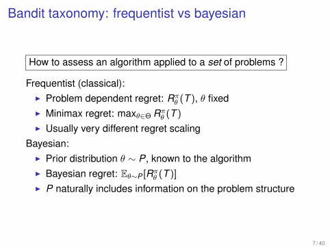
Bandit taxonomy: frequentist vs bayesian

How to assess an algorithm applied to a set of problems ?

Frequentist (classical):I Problem dependent regret: Rπ

θ (T ), θ fixedI Minimax regret: maxθ∈Θ Rπ

θ (T )

I Usually very different regret scalingBayesian:

I Prior distribution θ ∼ P, known to the algorithmI Bayesian regret: Eθ∼P [Rπ

θ (T )]

I P naturally includes information on the problem structure

7 / 40

Bandit taxonomy: cardinality of the set of armsDiscrete Bandits:

I X = {1, ...,K}I All arms can be sampled infinitely many timesI Regret O(log(T )) (stochastic), O(

√T ) (adversarial)

Infinite Bandits:I X = N, Bayesian setting (otherwise trivial)I Explore o(T ) arms until a good one is foundI Regret: O(

√T ).

Continuous Bandits:I X ⊂ Rd convex, x 7→ µθ(x) has a structureI Structures: convex, Lipshitz, linear, unimodal

(quasi-convex) etc.I Similar to derivative-free stochastic optimizationI Regret: O(poly(d)

√T ).

8 / 40

Bandit taxonomy: regret minimization vs best armidentification

Sample arms and output the best arm with a given probability,similar to PAC learning

Fixed budget setting:I T fixed, sample arms x1, ..., xT , and output x̂T

I Easier problem: estimation + budget allocationI Goal: minimize P[x̂T 6= x∗]

Fixed confidence setting:I δ fixed, sample arms x1, ..., xτ and output x̂τ

I Harder problem: estimation + budget allocation + optimalstopping (τ is a stopping time)

I Goal: minimize E[τ ] s.t. P[x̂T 6= x∗] ≤ δ

9 / 40

Example 1: Rate adaptation in wireless networks

I Adapting the modulation/coding scheme to the radioenvironment

I Rates: r1, r2 , . . . , rK

I Success probabilities: θ1, θ2 , . . . , θK

I Throughputs: µ1, µ2 , . . . , µK

Structure: unimodality + θ1 > θ2 > · · · > θK .

10 / 40

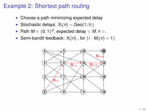
Example 2: Shortest path routing

I Choose a path minimizing expected delayI Stochastic delays: Xi(n) ∼ Geo(1/θi)

I Path M ∈ {0,1}d , expected delay < M, θ >.I Semi-bandit feedback: Xi(n) , for {i : Mi(n) = 1}

11

1616

2

8

7

3

4 5

6

12

11

10

9 13

14

15

θ1,6

θ6,11 θ11,15

θ15,16

11 / 40

Example 3: Learning to Rank (search engines)I Given a query, N relevant items, L display slotsI A user is shown L items, scrolls down and selects the first

relevant itemI One must show the most relevant items in the first slots.I θn probability of clicking on item n (independence between

items is assumed)I Reward r(l) if user clicks on the l-th item, and 0 if the user

does not click

Environ 171 000 000 résultats (0,31 secondes)

Signaler des images inappropriées

Autres résultats sur jaguar.fr »

Images correspondant à jaguar

Plus d'images pour jaguar

Dans l'actualité

Jaguar : une boîte manuelle pour la F-Typeen 2015Turbo.fr - Il y a 23 heures

La Jaguar F-Type est en train d'étoffer sa gamme après un

lancement en fanfare. D'abord ...

Plus d'actualités pour "jaguar"

Les cookies assurent le bon fonctionnement de nos services. En utilisant ces derniers, vousacceptez l'utilisation des cookies.

En savoir plus OK

Jaguar France - Voitures de Sport et Voitures de luxewww.jaguar.fr/Découvrez les voitures de luxe Jaguar. Alliant héritage et technologie, les berlines et

voitures de sport Jaguar vous feront vivre une expérience de conduite ...

F-TypeLa F-TYPE est une sportive

d'exception héritière de la lignée ...

Créez Votre JaguarCRÉEZ VOTRE JAGUAR. Nous

faisons tout notre possible pour ...

XELe pedigrée de la XE se lit dans ses

lignes, dans sa tenue de ...

XFJaguar XF, une gamme de Berlines

sportives au design et ...

Jaguar - Annonce Jaguar d'occasion - La Centralewww.lacentrale.fr/occasion-voiture-marque-jaguar.htmlJaguar occasion : annonces de Jaguar d'occasion. La Centrale s'engage : Annonces

securisees et de qualite pour la vente de Jaguar.

Jaguar (automobile) — Wikipédiafr.wikipedia.org/wiki/Jaguar_(automobile)Jaguar, de son nom officiel « Jaguar Cars Ltd », est une marque automobile britannique

connue pour ses voitures de luxe et ses modèles sportifs. La marque ...

Jaguar — Wikipédiafr.wikipedia.org/wiki/JaguarStatut de conservation UICN. ( NT ) NT : Quasi menacé. Statut CITES. Sur l'annexe I de

la CITES Annexe I , Rév. du 01-07-1975. Le jaguar (Panthera onca) est ...

Jaguar - Caradisiacwww.caradisiac.com › Toutes les marques

Constructeur automobile

Jaguar, de son nom officiel« Jaguar Cars Ltd », est une marqueautomobile britannique connue pour sesvoitures de luxe et ses modèles sportifs.Wikipédia

Date de fondation : septembre 1922,Blackpool, Royaume-Uni

PDG : Ralf Speth

Fondateurs : William Walmsley, WilliamLyons

Jaguar France74 abonnés • Partagé en modepublic

Découvrez lanouvelle #JaguarXES en action dans lesrues de Londres.#FEELXEhttp://fal.cn/KSE9 nov. 2014

Jaguar

Posts récents sur Google+

Commentaires

Afficher les résultats pourJaguar (Animal)Rang : EspèceClassification : Panthera

Web Images Actualités Vidéos Maps Outils de recherchePlus

jaguar Connexion

jaguar - Recherche Google https://www.google.fr/search?client=ubuntu&ch...

1 of 2 17/11/2014 11:49

12 / 40

Example 4: Ad-display optimization

I Users are shown ads relevant to their queriesI Announcers k ∈ {1, ...,K}, with µk click-through-rate and

budget per unit of time ck

I Bandit with budgets: each arm has a budget of playsI Displayed announcer is charged per impression/click

13 / 40

Outline

Introduction and examples of application

Tools and techniques

Discrete bandits with independent arms

14 / 40

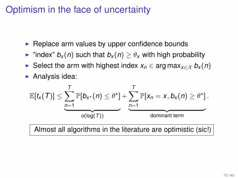
Optimism in the face of uncertainty

I Replace arm values by upper confidence boundsI ”index” bx (n) such that bx (n) ≥ θx with high probabilityI Select the arm with highest index xn ∈ arg maxx∈X bx (n)

I Analysis idea:

E[tx (T )] ≤T∑

n=1

P[bx?(n) ≤ θ?]︸ ︷︷ ︸o(log(T ))

+T∑

n=1

P[xn = x ,bx (n) ≥ θ?]︸ ︷︷ ︸dominant term

.

Almost all algorithms in the literature are optimistic (sic!)

15 / 40

Information theory and statisticsI Distribtions P,Q with densities p and q w.r.t a measure mI Kullback-Leibler divergence:

D(P||Q) =

∫x

p(x) log(

p(x)

q(x)

)m(dx),

I Pinsker’s inequality:

D(P||Q) ≥ 12

∫x|p(x)− q(x)|m(dx).

I If P,Q ∼ Ber(p), Ber(q):

D(P||Q) = p log(

pq

)+ (1− p) log

(1− p1− q

)I Also (Pinkser + inequality log(x) ≤ x − 1):

2(p − q)2 ≤ D(P||Q) ≤ (p − q)2

q(1− q)

The KL-divergence is ubiquitous in bandit problems

16 / 40

Empirical divergence and Sanov’s inequality

I P a discrete distribution with support PI P̂n empirical distribution of an i.i.d sample of size n from P,I Sanov’s inequality:

P[D(P̂n||P) ≥ δ] ≤(

n + |P| − 1|P|+ 1

)e−nδ

I Suggests confidence regions (risk α) of the type:

{P : n D(P̂n||P) ≤ log(1/α)}

17 / 40

Hypothesis testing and sample complexity

I How many samples are needed to distinguish P from Q ?I Observe X = (X1, ...,Xn) i.i.d with distribution Pn or Qn

I Additivity of the KL divergence: D(Pn||Qn) = nD(P||Q)

I Test φ(X ) ∈ {0,1}, risk α > 0:

EP [φ(X )] + EQ[1− φ(X )] ≤ α

I Tsybakov’s inequality:

(1/2)e−min{D(Pn||Qn),D(Qn||Pn)} ≤ EP [φ(X )] + EQ[1− φ(X )]

I Minimal number of samples:

n ≥ log(1/α)− log(2)

min{D(P||Q),D(Q||P)}

18 / 40

Regret Lower Bounds: general technique

I Decision x , two parameters θ, λ, with x?(λ) = x 6= x?(θ).I Consider consider an algorithm with Rπ(T ) = log(T ) for all

parameters (unformly good):

Eθ[tx (T )] = O(log(T )) , Eλ[tx (T )] = T −O(log(T )).

I Markov inequality:

Pθ[tx (T ) ≥ T/2] + Pλ[tx (T ) < T/2] ≤ O(T−1 log(T )).

I 1{tx (T ) ≤ T/2} is a hypothesis test, risk O(T−1 log(T ))

I Hence (Neyman-Pearson / Tsybakov):∑x

Eθ[tx (T )]I(θx , λx )︸ ︷︷ ︸KL divergence of the observations

≥ log(T )−O(log(log(T ))).

19 / 40

Concentration inequalities: Chernoff bounds

I Building indexes requires tight concentration inequalitiesI Chernoff bounds: upper bound the MGFI X = (X1, ...,Xn) independent, with mean µ, Sn =

∑nn′=1 Xn′

I G such that log(E[eλ(Xn−µ)]) ≤ G(λ) , λ ≥ 0I Generic technique:

P[Sn − nµ ≥ δ] = P[eλ(Sn−nµ) ≥ eλδ]

≤ e−λδE[eλ(Sn−nµ)] (Markov)= exp(nG(λ)− λδ) (independence)

≤ exp(−n max

λ≥0{λδn−1 −G(λ)}

).

20 / 40

Concentration inequalities: Chernoff and Hoeffding’sinequality

I Bounded variables: if Xn ∈ [a,b] a.s thenE[eλ(Xn−µ)] ≤ eλ

2(b−a)2/8 (Hoeffding lemma)I Hoeffding’s inequality:

P[Sn − nµ ≥ δ] ≤ exp(− 2δ2

n(b − a)2

)I Subgaussian variables: E[eλ(Xn−µ)] ≤ eσ

2λ2/2, similar

I Bernoulli variables: E[eλ(Xn−µ)] = µeλ(1−µ) − (1− µ)e−λµ

I Chernoff’s inequality:

P[Sn − nµ ≥ δ] ≤ exp(−nI(µ+ δ/n, µ))

I Pinsker’s inequality: Chernoff is stronger than Hoeffding.

21 / 40

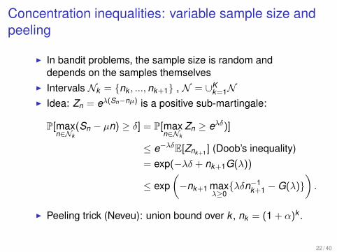
Concentration inequalities: variable sample size andpeeling

I In bandit problems, the sample size is random anddepends on the samples themselves

I Intervals Nk = {nk , ...,nk+1} , N = ∪Kk=1N

I Idea: Zn = eλ(Sn−nµ) is a positive sub-martingale:

P[maxn∈Nk

(Sn − µn) ≥ δ] = P[maxn∈Nk

Zn ≥ eλδ)]

≤ e−λδE[Znk+1 ] (Doob’s inequality)= exp(−λδ + nk+1G(λ))

≤ exp(−nk+1 max

λ≥0{λδn−1

k+1 −G(λ)}).

I Peeling trick (Neveu): union bound over k , nk = (1 + α)k .

22 / 40

Concentration inequalities: self normalized versions

I Self-normalized versions of classical inequalitiesI Garivier’s inequality:

P[

max1≤n≤T

nI(Sn/n, µ) ≥ δ]≤ 2edlog(T )δee−δ

I From Pinkser’s inequality (self-normalized Hoeffding):

P[

max1≤n≤T

√n|Sn/n − µ| ≥ δ

]≤ 4edlog(T )δ2ee−2δ2

I Multi-dimensional version, Y knk

= nk I(Snk/nk , µ)

P

[max

(n1,...,nK )∈[1,T ]K

K∑k=1

Y knk≥ δ

]≤ CK (log(T )δ)K e−δ

23 / 40

Outline

Introduction and examples of application

Tools and techniques

Discrete bandits with independent arms

24 / 40

The Lai-Robbins bound

I Actions X = {1, ...,K}I Rewards θ = (θ1, ..., θK ) ∈ [0,1]K

I Uniformly good algorithm: R(T ) = O(log(T )) , ∀θ

Theorem (Lai ’85)

For any uniformly good algorithm, and x s.t θx < θ? we have:

lim infT→∞

E[tx (T )]

log(T )≥ 1

I(µx , µ?)

I For x 6= x?, apply the generic technique with:

λ = (θ1, ..., θx−1, θ? + ε, θx+1, ..., θK )

25 / 40

The Lai-Robbins bound

θx

x

Most confusing parameter

26 / 40

Optimistic Algorithms

I Select the arm with highest index k(n) ∈ arg maxk bk (n)

I UCB algorithm (Hoeffding’s ineqality):

bx (n) = θ̂x (n)︸ ︷︷ ︸empirical mean

+

√2 log(n)

tx (n)︸ ︷︷ ︸exploration bonus

.

I KL-UCB algorithm (Self-normalized Chernoff inequality):

bx (n) = max{q ≤ 1 : tx (n)I(θ̂x (n),q)︸ ︷︷ ︸likelihood ratio

≤ f (n)︸︷︷︸log(confidence level−1)

}.

with f (n) = log(n) + 3 log(log(n)).

27 / 40

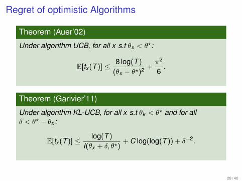
Regret of optimistic Algorithms

Theorem (Auer’02)

Under algorithm UCB, for all x s.t θx < θ?:

E[tx (T )] ≤ 8 log(T )

(θx − θ?)2 +π2

6.

Theorem (Garivier’11)

Under algorithm KL-UCB, for all x s.t θk < θ? and for allδ < θ? − θx :

E[tx (T )] ≤ log(T )

I(θx + δ, θ?)+ C log(log(T )) + δ−2.

28 / 40

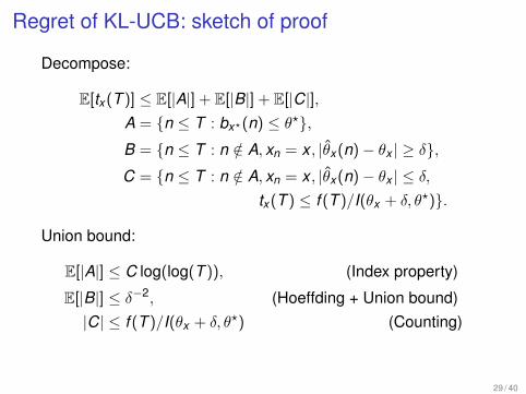
Regret of KL-UCB: sketch of proof

Decompose:

E[tx (T )] ≤ E[|A|] + E[|B|] + E[|C|],A = {n ≤ T : bx?(n) ≤ θ?},B = {n ≤ T : n /∈ A, xn = x , |θ̂x (n)− θx | ≥ δ},C = {n ≤ T : n /∈ A, xn = x , |θ̂x (n)− θx | ≤ δ,

tx (T ) ≤ f (T )/I(θx + δ, θ?)}.

Union bound:

E[|A|] ≤ C log(log(T )), (Index property)

E[|B|] ≤ δ−2, (Hoeffding + Union bound)|C| ≤ f (T )/I(θx + δ, θ?) (Counting)

29 / 40

Randomized algorithms: Thompson Sampling

I Prior distribution θ ∼ PI Time n, select x with probability

P[θx = maxx ′ θx ′ |x0, r0, ..., xn, rn]

Bernoulli with uniform priors:I Zx (n) ∼ Beta(tx (n)θ̂x (n) + 1, tx (n)(1− θ̂x (n)) + 1)

I xn+1 ∈ arg maxx Zx (n)

Theorem (Kaufmann’12)

Thompson sampling is asymptotically optimal. If θx < θ? then:

lim supT→∞

E[tx (T )]

log(T )≤ 1

I(θx , θ?).

30 / 40

Illustration of algorithms

−0.2 0 0.2 0.4 0.6 0.8 1 1.20

0.2

0.4

0.6

0.8

1

1.2UCB

µ̂1(n)

n = 102 t(n) = (20, 29, 54)

µ̂2(n)

n = 102 t(n) = (20, 29, 54)

µ̂3(n)n = 102 t(n) = (20, 29, 54)

−0.2 0 0.2 0.4 0.6 0.8 1 1.20

0.2

0.4

0.6

0.8

1

1.2KL−UCB

µ̂1(n)

n = 102 t(n) = (2, 5, 96)

µ̂2(n)

n = 102 t(n) = (2, 5, 96)

µ̂3(n)n = 102 t(n) = (2, 5, 96)

10 20 30 40 50 60 70 80 90 1000

5

10

15

Regret of various algorithms

Time T

Reg

ret R

(T)

UCBKL−UCBThompson

31 / 40

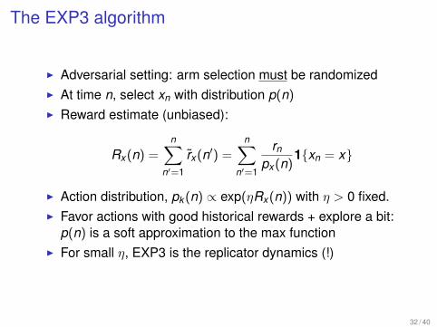
The EXP3 algorithm

I Adversarial setting: arm selection must be randomizedI At time n, select xn with distribution p(n)

I Reward estimate (unbiased):

Rx (n) =n∑

n′=1

r̃x (n′) =n∑

n′=1

rn

px (n)1{xn = x}

I Action distribution, pk (n) ∝ exp(ηRx (n)) with η > 0 fixed.I Favor actions with good historical rewards + explore a bit:

p(n) is a soft approximation to the max functionI For small η, EXP3 is the replicator dynamics (!)

32 / 40

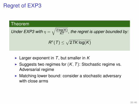
Regret of EXP3

Theorem

Under EXP3 with η =√

2 log(K )KT , the regret is upper bounded by:

Rπ(T ) ≤√

2TK log(K )

I Larger exponent in T , but smaller in KI Suggests two regimes for (K ,T ): Stochastic regime vs.

Adversarial regimeI Matching lower bound: consider a stochastic adversary

with close arms

33 / 40

BibliographyDiscrete bandits- Thompson, On the likelihood that one unknown probabilityexceeds another in view of the evidence of two samples, 1933- Robbins, Some aspects of the sequential design ofexperiments, 1952- Lai and Robbins. Asymptotically efficient adaptive allocationrules, 1985- Lai. Adaptive treatment allocation and the multi-armed banditproblem, 1987- Gittins, Bandit Processes and Dynamic Allocation Indices,1989- Auer, Cesa-Bianchi and Fischer, Finite time analysis of themultiarmed bandit problem. 2002.- Garivier and Moulines, On upper-confidence bound policiesfor non-stationary bandit problems, 2008- Slivkins and Upfal, Adapting to a changing environment: thebrownian restless bandits, 2008

34 / 40

Bibliography

- Garivier and Cappé. The KL-UCB algorithm for boundedstochastic bandits and beyond, 2011- Honda and Takemura, An Asymptotically Optimal BanditAlgorithm for Bounded Support Models, 2010

Discrete bandits with correlated arms

- Anantharam, Varaiya, and Walrand, Asymptotically efficientallocation rules for the multiarmed bandit problem with multipleplays, 1987- Graves and Lai Asymptotically efficient adaptive choice ofcontrol laws in controlled Markov chains, 1997- György, Linder, Lugosi and Ottucsák, The on-line shortestpath problem under partial monitoring, 2007- Yu and Mannor, Unimodal bandits, 2011- Cesa-Bianchi and Lugosi, Combinatorial bandits, 2012.

35 / 40

Bibliography- Gai, Krishnamachari, and Jain, Combinatorial networkoptimization with unknown variables: Multi-armed bandits withlinear rewards and individual observations, 2012- Chen, Wang and Yuan. Combinatorial multi-armed bandit:General framework and applications, 2013- Combes and Proutiere, Unimodal bandits: Regret lowerbounds and optimal algorithms, 2014- Magureanu, Combes, and Proutiere. Lipschitz bandits: Regretlower bounds and optimal algorithms, 2014.

Thompson Sampling

- Chapelle and Li, An Empirical Evaluation of ThompsonSampling, 2011- Korda, Kaufmann and Munos, Thompson Sampling: anasymptotically optimal finite-time analysis, 2012- Korda, Kaufmann and Munos, Thompson Sampling forone-dimensional exponential family bandits, 2013.

36 / 40

Bibliography- Agrawal and Goyal, Further optimal regret bounds forThompson Sampling, 2013.- Agrawal and Goyal, Thompson Sampling for contextualbandits with linear payoffs, June 2013.

Discrete adversarial bandits

- Auer, Cesa-Bianchi, Freund and Schapire, The non-stochasticmulti-armed bandit, 2002

Continuous Bandits (Lipschitz)

- R. Agrawal, The continuum-armed bandit problem, 1995- Auer, Ortner, and Szepesvári, Improved rates for thestochastic continuum-armed bandit problem, 2007- Bubeck, Munos, Stoltz, and Szepesvári, Online optimization inx-armed bandits, 2008

37 / 40

Bibliography- Kleinberg. Nearly tight bounds for the continuum-armedbandit problem, 2004- Kleinberg, Slivkins, and Upfal, Multi-armed bandits in metricspaces, 2008- Bubeck, Stoltz and Yu, Lipschitz bandits without the Lipschitzconstant, 2011

Continuous Bandits (strongly convex)

- Cope, Regret and convergence bounds for a class ofcontinuum-armed bandit problems, 2009- Flaxman, Kalai, and McMahan, Online convex optimization inthe bandit setting: gradient descent without a gradient, 2005- Shamir, On the complexity of bandit and derivative-freestochastic convex optimization, 2013- Agarwal, Foster, Hsu, Kakade, and Rakhlin, Stochasticconvex optimization with bandit feedback, 2013.

38 / 40

BibliographyContinuous Bandits (linear)

- Dani, Hayes, and Kakade, Stochastic linear optimizationunder bandit feedback, 2008- Rusmevichientong and Tsitsiklis, Linearly ParameterizedBandits, 2010- Abbasi-Yadkori, Pal, Szepesvári, Improved Algorithms forLinear Stochastic Bandits, 2011

Best Arm identification

- Mannor and Tsitsiklis, The sample complexity of exploration inthe multi-armed bandit problem, 2004- Even-Dar, Mannor, Mansour, Action elimination and stoppingconditions for the multi-armed bandit and reinforcementlearning problems, 2006- Audibert, Bubeck, and Munos, Best arm identification inmulti-armed bandits, 2010. 39 / 40

Bibliography

- Kalyanakrishnan, Tewari, Auer, and Stone, Pac subsetselection in stochastic multi-armed bandits, 2012- Kaufmann and Kalyanakrishnan, Information complexity inbandit subset selection, 2013- Kaufmann, Garivier and Cappé, On the Complexity of A/BTesting, 2014

Infinite Bandits

- Berry, Chen, Zame, Heath, and Shepp, Bandit problems withinfinitely many arms, 1997.- Wang, Audibert, and Munos, Algorithms for infinitelymany-armed bandits, 2008.- Bonald and Proutiere, Two-Target Algorithms forInfinite-Armed Bandits with Bernoulli Rewards, 2013

40 / 40