Polynomiography: A New Intersection between Mathematics and Art 1

Bahman Kalantari

Department of Computer Science, Rutgers UniversityHill Center, New Brunswick, NJ, 08903

Polynomiography is defined to be “the art and science of visualization in approximation ofthe zeros of complex polynomials, via fractal and non-fractal images created using the mathe-matical convergence properties of iteration functions.” An individual image is called a “poly-nomiograph.” The word polynomiography is a combination of the word “polynomial” and thesuffix “-graphy.” It is meant to convey the idea that it represents a certain graph of poly-nomials, but not in the usual sense of graphing, say a parabola for a quadratic polynomial.Polynomiographs are obtained using algorithms requiring the manipulation of thousands ofpixels on a computer monitor. Depending upon the degree of the underlying polynomial, it ispossible to obtain beautiful images on a laptop computer in less time than a TV commercial.

Polynomials form a fundamental class of mathematical objects with diverse applications;they arise in devising algorithms for such mundane task as multiplying two numbers, muchfaster than the ordinary way we have all learned to do this task (FFT). According to theFundamental Theorem of Algebra, a polynomial of degree n, with real or complex coefficients,has n zeros (roots) which may or may not be distinct. The task of approximation of the zeros ofpolynomials is a problem that was known to Sumerians (third millennium B.C.). This problemhas been one of the most influential problem in the development of several important areas inmathematics. Polynomiography offers a new approach to solve and view this ancient problem,while making use of new algorithms and today’s computer technology. Polynomiography isbased on the use of one or an infinite number of iteration functions designed for the purposeof approximation of the roots of polynomials. An iteration function is a mapping of the planeinto itself, i.e. given any point in the plane, it is a rule that provides another point in the plane.Newton’s iteration function is the best known : N(z) = z − p(z)/p′(z). An iteration functioncan be viewed as a machine that approximates a zero of a polynomial by an iterative processthat takes an input and from it creates an output which in turn becomes a new input to thesame machine.

The word “fractal,” which partially appears in the definition of polynomiography, was coinedby the world-renowned research scientist Benoit Mandelbrot. It refers to sets or geometricobjects that are self-similar and independent of scale. This means there is detail on all levels ofmagnification. No matter how many times one zooms in, one can still discover new details. Itturns out that some fractal images can be obtained via simple iterative schemes leading to setsknown as Julia sets and the famous Mandelbrot set. The simplicity of these iterative schemes,which may or may not have any significant purpose in mind, has resulted in the creation ofnumerous web sites in which amateurs and experts exhibit their fractal images. Many fractalimages pertain to the famous Mandelbrot set.

Polynomiography, on the other hand, has a well-defined and focused purpose in mind.It makes use of one or an infinite number of iteration functions for polynomial root-finding.

1 c©2000 Bahman Kalantari. All Rights Reserved

1

A polynomiograph may or may not result in a fractal image. This is one of the reasons itwas necessary to give a new name to this process. A second reason is because its purposeis the visualization of a polynomial, via approximation of its roots and the way in whichthe approximation is carried out. Even when a polynomiograph is a fractal image it does notdiminish its uniqueness. The assertion that an image is a fractal image is no more profound thanasserting that an image is a picture, or a painting. In particular, that assertion does not captureany artistic values of the image. Indeed, even in terms of fractal images polynomiography revealsa vast number of possibilities and degrees of freedom and results in a wider variety of imagesthan typical fractal images.

Polynomiography could become a new art form. Working with polynomiography softwareis comparable to working with a camera or a musical instrument. Through practice, one canlearn to produce the most exquisite and complex patterns. These designs, at their best, areanalogous to the most sophisticated human designs. The intricate patterning of Islamic art,the composition of Oriental carpets, or the elegant design of French fabrics come to mindas very similar to the symmetrical, repetitive, and orderly graphic images produced throughpolynomiography. But polynomiographic designs can also be irregular, asymmetric, and non-recurring, suggesting parallels with the work of artists associated with Abstract Expressionismand Minimalism. Polynomiography could be used in classrooms for the teaching of art ormathematics, from children to college-level students, as well as in both professional and non-professional situations. Its creative possibilities could enhance the professional art curriculum.

The “polynomiographer” can create an infinite variety of designs. This is made possibleby employing an infinite variety of iteration functions (which are analogous to the lenses ofa camera) to the infinite class of complex polynomials (which are analogous to photographicmodels). The polynomiographer then may go through the same kind of decision making asthe photographer: changing scale, isolating parts of the image, enlarging or reducing, adjustingvalues and colors until the polynomiograph is resolved into a visually satisfying entity. Likea photographer, a polynomiographer can learn to create images that are esthetically beautifuland individual, with or without the knowledge of mathematics or art. Like an artist and apainter, a polynomiographer can be creative in coloration and composition of images. Like acamera, or a painting brush, a polynomiography software can be made simple enough that evena child could learn to operate it.

Despite the significant role of the root-finding problem in the development of fundamentalareas, today it is not considered to be a central problem in pure or computational mathematics.According to a 1997 article in SIAM Review by Victor Pan [28], a leading authority on thecomputational complexity aspects of the root-finding problem, in practice often one needs tocompute roots of polynomials of very moderate degree (10 or 20), except possibly in computeralgebra which is applied to algebraic optimization and algebraic geometry. In view of the aboveand since there are already efficient subroutines for computing roots of moderate size polynomi-als, it would not be surprising that many may view the polynomial root-finding problem as onethat has basically reached a dead-end. However, I believe that polynomiography will changeall of this, not only from the mathematical or scientific point of view, but from the educationaland artistic point of view.

Quoting the great American mathematician Smale [34], “There is a sense in which an im-portant result in mathematics is never finished.” The Fundamental Theorem of Algebra is oneof those results. To me polynomiography is a good evidence in support of Smale’s statement.With the availability of a good polynomiography software, the user (who may be a high schoolstudent, an artist, or a scientist) is quite likely to wish to experiment with much larger degreepolynomials than degree 10 or 20. In particular, this is true because in polynomiography there

2

is a “reverse root-finding problem”: given a polynomial whose roots form a known set of points,find an iteration method whose corresponding polynomiograph would take a desired pattern.In principle, using this reverse problem, I can conceive of the blue print to some of the mostelegant patterns, for instance carpets designs, yet to be woven. Their complexity and beautycould very well increase by increasing the degree size. Thus, it is conceivable that the imple-mentation of such designs would demand working with much more computer power than thatoffered by a laptop computer, perhaps a supercomputer, or a network of computers.

Mathematical Foundation of Polynomiography

Consider the polynomial

p(z) = anzn + an−1zn−1 + · · · + a1z + a0,

where n ≥ 2, and the coefficients a0, . . . , an are complex numbers. The problem of approximat-ing the roots of p(z) is a fundamental and classic problem. A large bibliography can be found in[25]. For an article on some history, applications, and new algorithms, see Pan [28]. Some of theroot-finding methods first obtain a high-precision approximation to a root, then approximateother roots after deflation, see e.g., Jenkins and Traub [10]. Many such root-finding methodsmake use of iteration functions, e.g. Newton’s or Laguerre’s. A method that guarantees con-vergence to all the roots was given by Weyl [38]. This method is a two-dimensional analogueof the bisection method. Modifications of this method has been used to obtain an initial ap-proximation to a root, followed by the use of Newton’s method with a guaranteed estimate onthe complexity of approximation, see e.g. Renegar [31], Pan [27]. Another root-finding methodis based on recursive factorization of the given polynomial, see e.g. Kirrin [23]. Many deeptheoretical complexity results on polynomial root-finding and/or the use of Newton’s method,are known, see e.g. Smale [34, 35], Shub and Smale [32, 33], Friedman [6]. Many topics onpolynomials can be found in [1], and [2].

One of the conceptually easiest algorithms for the approximation of all the roots of polyno-mials is described in Kalantari [20], making use of a fundamental family of iteration functionscalled the “Basic Family.” The algorithm reveals a magical pointwise convergence of the familyto roots (see Theorem 2). The Basic Family is represented as {Bm(z)}∞m=2. The algebraicdevelopment and some optimal properties of the Basic Family are studied in [12], [13]. Thefirst member of the sequence, B2(z), is Newton’s iteration function, and B3(z) is Halley’s iter-ation function [9]. For the rich history of these two iteration functions alone see Ypma [39] andTraub [36]. In particular, Halley’s method inspired the celebrated Taylor’s Theorem (see [39]).Many results on the properties of the members of this family including their close ties with adeterminantal generalization of Taylor’s Theorem can be found in [12]-[22].

The members of the Basic Family have an interesting closed formula. Let p(z) be a poly-nomial of degree n ≥ 2 with complex coefficients. Set D0(z) ≡ 1, and for each natural numberm ≥ 1, define

Dm(z) = det

p′(z) p′′(z)2! . . . p(m−1)(z)

(m−1)!p(m)(z)

(m)!

p(z) p′(z). . . . . . p(m−1)(z)

(m−1)!

0 p(z). . . . . .

......

.... . . . . . p′′(z)

2!0 0 . . . p(z) p′(z)

,

3

Dm,i(z) = det

p′′(z)2!

p′′′(z)3! . . . p(m)(z)

(m)!p(i)(z)

i!

p′(z) p′′(z)2!

. . . p(m−1)(z)(m−1)!

p(i−1)(z)(i−1)!

p(z) p′(z). . .

......

......

. . . p′′(z)2!

p(i−m+2)(z)(i−m+2)!

0 0 . . . p′(z) p(i−m+1)(z)(i−m+1)!

,

where i = m + 1, . . . , n + m − 1, and det(·) represents determinant.For each m ≥ 2, define

Bm(z) ≡ z − p(z)Dm−2(z)Dm−1(z)

.

Note that Dm(z) corresponds to the determinant of a Toeplitz matrix defined with respectto the normalized derivatives of p(z). A square matrix is called Toeplitz if its elements areidentical along each diagonal.

Some of the fundamental properties of the members of the Basic Family are described inthe following theorem. Its second part, in particular is a very special case of a nontrivialdeterminantal generalization of Taylor’s theorem given in [15].

Let C be the field of complex numbers. For a complex number c = a + ib, where i =√−1,

its modulus is |c| =√

a2 + b2.Theorem 1. Kalantari [16, 20]) The following conditions hold:

1. For all m ≥ 1 we have,

Dm(z) =n∑

i=1

(−1)i−1 pi−1(z)p(i)(z)i!

Dm−i(z), Dj = 0, j < 0.

2. Let θ be a simple root of p(z). Then,

Bm(z) = θ +m+n−2∑

i=m

(−1)mDm−1,i(z)Dm−1(z)

(z − θ)i.

3. There exists r > 0 such that given any a0 ∈ Nr(θ) = {z : |z − θ| ≤ r}, the fixed-pointiteration ak+1 = Bm(ak) is well-defined, and it converges to θ having order m. Specifically,

limk→∞

(θ − ak+1)(θ − ak)m

= (−1)m−1 Dm−1,m(θ)p′(θ)m−1

.

4. Let θ be a simple root of p(z). There exists a neighborhood of θ, N∗(θ), such that foreach a within this neighborhood p′(a) 6= 0, |a − θ| < 1, and

|p′(a)| −n∑

i=0,i6=1

|p(a)| i−12|p(i)(a)|

i!≥ 1

2|p′(a)|.

For any a ∈ N∗(θ), if we set

h(a) =[ n∑

i=0

( |p(i)(a)|i!

)2]1/2

,

4

then we have

|Bm(a) − θ| ≤∣∣∣∣2h(a)p′(a)

(a − θ)∣∣∣∣m

(1

1 − |a − θ|)

.

5. In particular, if θ is a simple root of p(z), there exists r∗ ∈ (0, 1) such that given anya ∈ Nr∗(θ), we have

θ = limm→∞Bm(a).

6. Dm(a) and hence Bm(a) can be computed in O(n log n log m) operations.

To describe a fundamental global convergence property of the sequence let

Rp = {θ1, . . . , θt}

be the set of distinct roots of p(z). The elements of Rp partition the Euclidean plane intoVoronoi regions and their boundaries. The Voronoi region of a root θ is a convex polygondefined by the locus of points which are closer to this root than to any other root. Moreprecisely, the Voronoi region of a root θ is

V (θ) = {z ∈ C : |z − θ| < |z − θ′|, ∀ θ′ ∈ Rp, θ′ 6= θ}.

Let Sp be the locus of points that are equidistant from two distinct roots, i.e.

Sp = {z ∈ C : |z − θ| = |z − θ′|, where θ, θ′ ∈ Rp, θ 6= θ′}.

This is a set of measure zero consisting of the union of a finite number of lines.Definition 1. Given a ∈ C the Basic Sequence at a is defined as

Bm(a) = a − p(a)Dm−2(a)Dm−1(a)

, m = 2, 3, . . . .

Theorem 2. ([20]) Given p(z), for any input a 6∈ Sp, the Basic Sequence is well-definedsatisfying

limm→∞Bm(a) = θ,

for some θ ∈ Rp. Under some regularity assumptions, e.g. simplicity of all the roots of p(z),for all a ∈ V (θ), limm→∞ Bm(a) = θ.

Remark. The determinantal generalization of Taylor’s theorem given in part 2 of Theorem1 gives a mechanism for estimating the error |Bm(a) − θ|. The Basic Sequence can be evendefined for functions that are not polynomial. In Kalantari [19] the pointwise evaluation of theBasic Family (the Basic Sequence in the terminology of Definition 1) is used to give new for-mulas for the approximation of π and e. In Kalantari [20] it is also shown how the relationshipbetween the Basic Sequence and the Basic Family gives new results for general homogeneouslinear recurrence relations that are defined via a single nonzero initial condition.

Basins of Attraction and Voronoi Regions of Polynomial Roots

Consider a polynomial p(z) and a fixed natural number m ≥ 2. The basins of attractionof a root of p(z) with respect to the iteration function Bm(z) are regions in the complex planesuch that given an initial point a0 within them, the corresponding sequence ak+1 = Bm(ak),k = 0, 1, . . . , will converge to that root. It turns out that the boundary of the basins of

5

attractions of any of the polynomial roots is the same set. This boundary is known as theJulia set and its complement it known as the Fatou set. The fractal nature of Julia sets andthe images of the basins of attraction of Newton’s method are now quite familiar for somespecial polynomials. For example fractal image of p(z) = z3 − 1 was apparently first studiedby the American mathematician John Hubbard while teaching calculus in France (see Gleick[8]). That image and similar images that are now quite familiar also appear in [26], as well as[37] (see also its references). Mandelbrot’s work (see The Fractal Geometry of Nature [24]) inparticular popularized the Julia theory [11] on the iteration of rational complex functions, aswell as the work of Fatou [5], and led to the famous set that bears Mandelbrot’s name. Peitgenet al. [30] undertake a further analysis of fractals. Mathematical analysis of complex iterationsmay be found in Peitgen and Richter [29], Devaney [3], and Falconer [4].

While the fractal nature of the Julia sets corresponding to the individual members of theBasic Family follows from the Julia theory on rational iteration functions, that theory does notpredict the total behavior of specific iteration functions on the complex plane. For instance theJulia theory does not even predict the shapes of basins of attraction of the polynomial p(z) =zn − 1 for various members of the Basic Family. In contrast, there are important consequencesof the results stated in Theorems 1 and 2 which apply to arbitrary polynomials. In particular,Theorem 2 implies the following: Except possibly for the locus of points equidistant to twodistinct roots, given any input a, the Basic Sequence {Bm(a) = a − p(a)Dm−2(a)/Dm−1(a)}converges to a root of p(z). Under some regularity assumption (e.g. simplicity of the roots),for almost all inputs within the Voronoi polygon of a root, the corresponding Basic Sequenceconverges to that root. The Basic Sequence corresponds to the pointwise evaluation of theBasic Family. Theorem 2 gives rise to a new set of non-fractal polynomiographs with enormousbeauty.

Figure 1 and Figure 2 present several fractal images that confirm the theoretical convergenceresults: as m increases, the basins of attraction of the roots, as computed with respect to theiteration function Bm(z), rapidly converge to the Voronoi regions of the roots. Thus the regionswith chaotic behavior rapidly shrink to the boundaries of the Voronoi regions.

Figure 1 considers a polynomial with a random set of roots, depicted as dots. The figureshows the evolution of the basins of attraction of the roots to the Voronoi regions as m takes thevalues 2, 4, 10, and 50. Figure 2 shows the basins of attraction for the polynomials p(z) = z4−1,corresponding to different values of m. The roots of p(z) = z4 − 1 are the roots of unity andhence the Voronoi regions are completely symmetric. In these figures in the case of m = 2, i.e.Newton’s method, the basins of attraction are chaotic. However, these regions rapidly improveby increasing m.

Figure 1: Evolution of basins of attraction to Voronoi regions via Bm(z): random points,m = 2, 4, 10, 50 (left to right).

Polynomiography and Visual Arts

I will first describe some general techniques for the creation of polynomiographic images

6

Figure 2: Evolution of basins of attraction to Voronoi regions via Bm(z): p(z) = z4 − 1,m = 2, 3, 4, 50 (left to right).

and exhibit sample images obtained via a prototype software for polynomiography, as well asprovide an explanation of how some of these images were created. Subsequently, I will considerother applications of polynomiography.

General Techniques for Creating Artwork

In order to describe some general techniques for producing polynomiographic images I willfirst describe the capabilities of prototype polynomiography software we have developed. Thesoftware allows the user to create an image by inputing a polynomial through several means,e.g. by inputing its coefficients, or the location of its zeros. In one approach the user simplyinputs a parameter, m, as any natural number greater than one. The assignment of a valuefor m corresponds to the selection of Bm(z) as the underlying iteration function. This togetherwith the selection of a user-defined rectangular region and user-specified number of pixels,tolerance, as well as a variety of color mapping schemes enables the user to create an infinitenumber of basic polynomiographs. These polynomiographs turn out to be fractal images andcan subsequently be easily re-colored or zoomed in any number of times. A non-fractal andcompletely different set of images could result from the visualization of the root-finding processthrough the collective use of the Basic Family, i.e. the pointwise convergence property describedin Theorem 2. These images are enormously rich. In either type of image creation techniquethe user has a great deal of choices, e.g. the ability to re-color any selected regions using avariety of coloration schemes based on convergence properties.

Viewing polynomiography as an art form, one can list at least four general image creationtechniques.

(1) Like a photographer who shoots different pictures of a model and uses a variety of lenses,a polynomiographer can produce different images of the same polynomial and make use of avariety of iteration functions and zooming approaches until a desirable image is discovered.

(2) In this more creative approach an initial polynomiograph, possibly very ordinary, isturned into a beautiful image, based on the user’s choice of coloration, individual creativity,and imagination. This is analogous to carving a statue out of stone.

(3) The user employs the mathematical properties of the iteration functions, or the under-lying polynomial, or both (this is truly a marriage of art and mathematics).

(4) Images can be created as a collage of two or more polynomiographs produced throughany one of the previous three methods.

Many other image creation techniques are possible, either through artistic compositionalmeans, or through computer assisted design programs.

An Exhibition

7

This section presents an exhibition of some polynomiographic images that I have createdthrough the above four techniques. The reader may notice the diversity of these images. Inparticular, they contrast with literally hundreds of fractal images exhibited at web sites. Itshould be noted that the images displayed are not necessarily symmetric. These are given asFigure 3 - Figure 13. It should be mentioned that none of the images in the paper is displayedat its optimal size. Indeed the optimal size for the display of some of the images is poster size.This is because at that size we begin to see and appreciate the real complexity and detail ofthe images.

In the near future an interactive version of a polynomiography software will become availableat www.polynomiography.com, where the visitor will be able to input his/her own polynomialand obtain various polynomiographs.

Figure 3: “Cathedral”, “Eiffel Tower”, “Party on Brooklyn Bridge”

Figure 4: “Waltz”

With the exception of some of the images in the “Evolution of Stars and Stripes”, and in

8

Figure 5: “Mathematics of a Heart”, “Mona Lisa in 2001”, “Butterfly”

Figure 6: All Untitled

“Ms. Poly” all other images have resulted from a single input polynomial. In “Ms. Poly”all regions that depict different features come from a single polynomial, except for her lips,themselves a polynomiograph, which came from a different polynomial and were collaged.

The Making of “Mona Lisa in 2001”

A polynomial of degree 10 was used to produce the left polynomiograph in Figure 12. Thenas a result of zooming in on one of the significant parts of that image, the right image in Figure12 was obtained. A coloration of various layers resulted in the final image.

The Making of “Mathematics of a Heart”

One of the features of the software is to allow the user to enter a polynomial by placing thelocation of the roots on the working canvas of the computer monitor. The software then buildsthe polynomial from the roots. Subsequently, any one of the techniques can be applied. Theimage “Mathematics of a Heart” was produced by simply drawing a heart shape and then byapplying one of the techniques, together with personal coloration.

9

Figure 7: “Life and Death” (two views of the same polynomial)

Figure 8: “Acrobats”, “Happy Birthday Hal!!!”

The Making of “Evolution of Stars and Stripes”

The inspiration to create a polynomiographic image of the U.S. flag came from Jasper Johnspaintings of the flag. The first image was conceived by making use of the convergence prop-erties of the Basic Family and the fact that the basins of attraction converge to the Voronoiregions of the roots. The underlying polynomial for the first image is a polynomial of degree5 whose roots consist of five points on a vertical line. The second and third images are vari-ations of the first one. The star image was obtained from a single polynomial and is collaged(after reduction of size) onto the third image. The final image comes from the coloration of apolynomiograph of a single polynomial (zoomed in at an appropriate area) together with thecollage of white stars coming from a different polynomiograph than that of the evolving star.It is hoped that the five images give the impression that the flag is evolving: the appearance ofthe stripes and the emergence of the color white (first images); the close up of the first image,while the evolution is in progress, which reveals the emergence of the color blue (second image);the creation of stars and the continuous growth and reshaping of white and blue regions (thirdimage); a close-up of one of the forming stars which appear as if it is in rotation (fourth fig-ure); and finally the orderly formations of various components of the flag and the settling of thestars. The conceptualization and creation of the five images took more than the summer of 2000.

10

Figure 9: “Evolution of Stars and Stripes”

Figure 10: “Summer Variations”

Symmetric Designs from Polynomiography

Symmetric designs can be obtained by considering polynomials whose roots have symmetricpatterns. One can obtain interesting images by simply considering polynomials whose rootsare the roots of unity or more generally n-th root of a real number r. By the multiplicationof these polynomials, as well as the rotation of the roots one can obtain some very interestingbasic designs that can subsequently be painted into beautiful designs. The images in Figure 13and Figure 16 are such examples.

Polynomiographs of Numbers

One interesting application of polynomiography is in the encryption of numbers, e.g. IDnumbers or credit card numbers into a two dimensional image that resembles a fingerprint.Different numbers will exhibit different fingerprints. One way to visualize numbers as poly-nomiographs is to represent them as polynomials. For instance a hypothetical social securitynumber a8a7 · · · a0 can be identified with the polynomial P (z) = a8z

8 + · · · + a1z + a0. Nowwe can apply any of the techniques discussed earlier. A particularly interesting visualizationresults when the software makes use of the Basic Family collectively (see Theorem 2). Figures

11

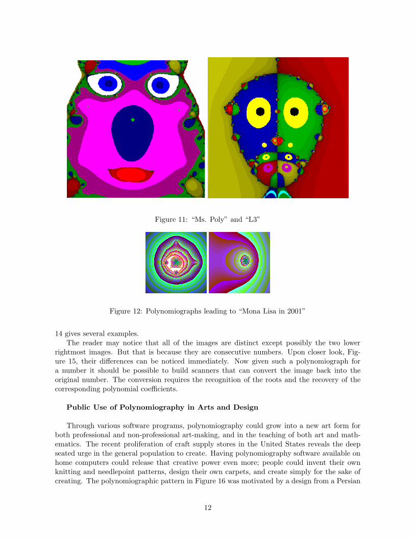
Figure 11: “Ms. Poly” and “L3”

Figure 12: Polynomiographs leading to “Mona Lisa in 2001”

14 gives several examples.The reader may notice that all of the images are distinct except possibly the two lower

rightmost images. But that is because they are consecutive numbers. Upon closer look, Fig-ure 15, their differences can be noticed immediately. Now given such a polynomiograph fora number it should be possible to build scanners that can convert the image back into theoriginal number. The conversion requires the recognition of the roots and the recovery of thecorresponding polynomial coefficients.

Public Use of Polynomiography in Arts and Design

Through various software programs, polynomiography could grow into a new art form forboth professional and non-professional art-making, and in the teaching of both art and math-ematics. The recent proliferation of craft supply stores in the United States reveals the deepseated urge in the general population to create. Having polynomiography software available onhome computers could release that creative power even more; people could invent their ownknitting and needlepoint patterns, design their own carpets, and create simply for the sake ofcreating. The polynomiographic pattern in Figure 16 was motivated by a design from a Persian

12

Figure 13: A polynomiograph of 10z48 − 11z24 + 1

carpet and made use of pointwise convergence described in Theorem 2. It is possible to obtainmuch more sophisticated patterns than this.

At a more advanced level, polynomiography can be used to teach the fundamentals of designand color theory. While information science software has transformed the advanced graphic de-sign curriculum through Photo Shop, Quark, and similar programs, the visual arts curriculummakes little use of information science at the fundamentals level. Polynomiography providesthe opportunity to teach decision-making in composition, spatial construction, and color at amuch more complex level than the present system which relies on the traditional methods ofdrawing and collage. Through using polynomiography software, students have infinite designpossibilities before them. In making their selections, they can experiment with symmetry andasymmetry, repetition, unity, balance, spatial illusion, lines, and planes. By using color, theycan gain understanding of complementary color, value relationships, and balance while learningto manipulate hue, tint, and intensity.

Polynomiography and Education

Polynomiography has enormous potential applications in education. A polynomiography

13

Figure 14: A polynomiograph of six different nine digit numbers

Figure 15: A polynomiograph of the numbers 672,123,450 and 672,123,451

software could be used in the mathematics classroom as a device for understanding polynomialsas well as the visualization of theorems pertaining to polynomials. As an example of oneapplication of polynomiography, high school students studying algebra and geometry could beintroduced to mathematics through creating designs from polynomials. They would learn touse algorithms on a sophisticated level and to understand the mathematics of polynomials intheir relationship to pattern and design in ways that cannot be approached abstractly. Forinstance, Figure 14 can be viewed as a visualization of the Fundamental Theorem of Algebra,as applied to the polynomials corresponding to these numbers. It is possible to compile manytheorems about polynomials and their properties, or those of iteration functions that can bevisualizable through polynomiography. At a higher educational level, e.g. calculus or numericalanalysis courses, polynomiography allows students to tackle important conceptual issues suchas the notion of convergence and limits, as well as the idea of iteration functions, and gives thestudent the ability to understand and appreciate more modern discoveries such as fractals.

There are also numerous algorithmic issues that are motivated by polynomiography, such asthe development of even newer root-finding algorithms. Polynomiography is not only a meansfor obtaining fast algorithms for polynomial root-finding but also allows the users to determinehow two particular members of the Basic Family compare. Which is better, Newton’s methodor Halley’s method? Most numerical analysis books do not bother with such questions. Butindeed these are fundamental questions from a pedagogical and practical point of view. Onemay make use of fractal images to study the computational advantages of members of the BasicFamily over Newton’s method, as well as the advantages in using the Basic Sequence in com-puting a single root, or all the roots of a given polynomial.

14

Figure 16: A polynomiograph of a degree 36 polynomial

Extensions of Polynomiography and Iteration Techniques

In this paper, polynomiography has been introduced in terms of the properties of a fun-damental family of iteration functions, namely the Basic Family. However, more generallypolynomiography can be defined with respect to any iteration function for polynomial root-finding. While experimentation with polynomiographs of other iteration functions is likely tobe interesting, many unique mathematical and computational properties of the Basic Familymembers makes them much more interesting than any other individual iteration function, and asa family more fundamental than any other family of iteration functions. There are still manymathematical properties of the family that need to be studied. Moreover, polynomiographycould even be enhanced with multipoint versions of the Basic Family.

A nontrivial determinantal generalization of Taylor’s formula proved in Kalantari [15], whoseprecise description is avoided here, plays a dual role in the approximation of a given functionor its inverse (hence its roots). On the one hand, the determinantal Taylor formula unfoldseach ordinary Taylor polynomial into an infinite spectrum of rational approximations to thegiven function. On the other hand, these formulas give an infinite spectrum of rational inverseapproximations, as well as single and multipoint iteration functions that include the BasicFamily. Given m ≥ 2, for each k ≤ m, we obtain a k-point iteration function, defined as theratio of two determinants that depend on the first m− k derivatives. These matrices are upperHessenberg and for k = 1 also reduce to Toeplitz matrices. The corresponding iteration functionis denoted by B

(k)m . Their formula will not be given here. Their order of convergence, proved

in Kalantari [14], ranges from m to the limiting ratio of the generalized Fibonacci numbers oforder m.

The following diagram represents the ascending order of convergence of B(k)m , and the cor-

responding orders for a partial table of iteration functions:

B(1)2 ← B

(2)2↓ ↓ ↘

B(1)3 ← B

(2)3 ← B

(3)3↓ ↓ ↓ ↘

B(1)4 ← B

(2)4 ← B

(3)4 ← B

(4)4↓ ↓ ↓ ↓ ↘

B(1)5 ← B

(2)5 ← B

(3)5 ← B

(4)5 ← B

(5)5↓ ↓ ↓ ↓ . . . ↘

2 ← 1.618↓ ↓ ↘3 ← 2.414 ← 1.839↓ ↓ ↓ ↘4 ← 3.302 ← 2.546 ← 1.927↓ ↓ ↓ ↓ ↘5 ← 4.236 ← 3.383 ← 2.592 ← 1.965↓ ↓ ↓ ↓ . . . ↘

15

The Basic Family is only the first column of the above diagram. The practicality of themultipoints was considered in [22] which gave a computational study of the first nine root-finding methods. These include the Newton, secant, and Halley methods. Our computationalresults with polynomials of degree up to 30 revealed that for small degree polynomials B

(k−1)m is

more efficient than B(k)m , but as the degree increases, B

(k)m becomes more efficient than B

(k−1)m .

The most efficient of the nine methods is the derivative-free method B(4)4 , having a theoretical

order of convergence equal to 1.927. Newton’s method which is often viewed as the method ofchoice is in fact the least efficient method. More computational results and a bigger subset ofthe above infinite table could reveal further practicality of the multipoint iteration family.

The properties of the Basic Family and the Basic Sequence give rise to new algorithmicstrategies. When the given input a is close enough to a simple root of the underlying polyno-mial, for any m ≥ 2, the Basic Sequence can be turned into an iterative method of order m byreplacing the given input a with Bm(a), and repeating. There are many computational impli-cations of these results. As an example, one possible algorithm for polynomial root-finding isthe following: for a given input a continue producing Bm(a) until the difference between Bm(a)and Bm+1(a) is small. Then for a desirable m replace a with Bm(a) and repeat in order toobtain higher and higher accuracy. It is also possible to switch back and forth between the twoschemes.

An algorithm suggested by the global convergence properties of the Basic Sequence in orderto compute all the roots of a given polynomial is as follows: first we obtain a rectangle thatcontains all the roots. Then, by selecting a sparse number of points we generate the corre-sponding Basic Sequence and thereby obtain a good approximation to a subset of the roots.Then after deflation the same approach can be applied to find additional roots. This methodcould provide an excellent alternative to the method of Weyl [38] (see also Pan [28] for Weyl’smethod). Experimentation with this method is intended and will be reported in the future.

In addition to the above multipoint versions of the Basic Family, it is also possible to de-fine an infinite “Truncated Basic Family,” as well as a “parameterized Basic Family.” Doingpolynomiography with these will be the subject of future work. It would also be interesting toconsider polynomiography with other families of iteration functions, e.g. the Euler-Schroederfamily (see [13], [15]).

Concluding Remarks and the Future of Polynomiography

In this paper I have described some general techniques for creating polynomiographic images.However, even with polynomiography software at one’s disposal, from the user’s point of viewit is essential to have available a very detailed and systematic manual and/or a book. Thecreation of such publications is one of my future goals. Indeed different users will benefit fromdifferent such publications.

It is believed that through various software programs polynomiography could not only growinto a new art form for both professional and non-professional art-making, but also into a toolwith enormous applications in the teaching of art and mathematics. One polynomiographysoftware can be used to teach both art and mathematics more effectively; and another can beused for the visualization of polynomial properties by advanced researchers. For instance, I canforesee that some mathematicians will become interested in studying the polynomiography ofmany important families of polynomials. Polynomiography can be used not only to teach aboutpolynomials and polynomial root-finding, but also about the underlying notions, e.g. complex

16

numbers and operations on them. Effective means of communications of artistic or educationalaspects of polynomiography can best be achieved by collaboration with artists, mathematicians,and educators. This is another of my future plans.

Polynomiography also provides a potentially powerful tool for architecture, furniture, andother kinds of design. Some two-dimensional polynomiographs can give rise to three-dimensionalobjects. These and other three-dimensional applications of polynomiography are yet anotherone of my future goals.

Finally, I remark that some convergence properties of the Basic Family are extendable tomore general analytic functions than polynomials. Thus, analogous to the case of polynomials,it is possible to visualize roots of these more general analytic functions. However, the efficiencyof the corresponding visualizations could dramatically decrease. For instance, applying thebasic family to a rational function (quotient of two polynomials) is inefficient as we make useof higher order members of the Basic Family. From the visual point of view, the world ofpolynomials is already infinitely rich. Moreover, polynomials form an important class, whichmakes them very appealing for conveying many concepts. One of my present goals is to design anew course on the subject of polynomiography with the aim of bringing together students fromart and science. While the title of this paper introduces polynomiography as an intersectionbetween mathematics and art, I do believe that it enhances both areas.

References

[1] D. Bini and V. Y. Pan, Polynomials and Matrix Computations, Vol. 1: Fundamental Algorithms,Birkhauser, Boston, Cambridge, MA, 1994.

[2] P. Borwein and T. Erdelyi, Polynomials and Polynomial Inequalities, Vol. 161, Springer-Verlag,New York, 1995.

[3] R. L. Devaney, Introduction to Chaotic Dynamic Systems, Benjamin Cummings, 1986.

[4] K. J. Falconer, Fractal Geometry: Mathematical Foundations and Applications, John Wiley & Sons,1990.

[5] P. Fatou, Sur les equations fonctionelles, Bull. Soc. Math. France, 47 (1919), 161-271.

[6] J. Friedman, On the convergence of Newton’s method, J. of Complexity, 5 (1989), 12-33.

[7] J. Gerlach, Accelerated convergence in Newton’s method, SIAM Review, 36 (1994), 272-276.

[8] J. Gleick, Chaos: Making a New Science, Penguin Books, 1988.

[9] E. Halley, A new, exact, and easy method of finding roots of any equations generally, and thatwithout any previous reduction, Philos. Trans. Roy. Soc. London, 18 (1694), 136-145.

[10] M.A. Jenkins and J.F. Traub, A three-stage variable-shift iteration for polynomial zeros and itsrelation to generalized Rayleigh iteration, Numer. Math., 14 (1970), 252-263.

[11] G. Julia, Sur les equations fonctionelles, J. Math. Pure Appl., 4 (1918), 47–245.

[12] B. Kalantari, and I. Kalantari, High order iterative methods for approximating square roots, BIT36 (1996), 395-399.

[13] B. Kalantari, I. Kalantari, and R. Zaare-Nahandi, A basic family of iteration functions for polyno-mial root finding and its characterizations, J. of Comp. and Appl. Math., 80 (1997), 209-226.

[14] B. Kalantari, On the order of convergence of a determinantal family of root-finding methods, BIT39 (1999), 96-109.

17

[15] B. Kalantari, Generalization of Taylor’s theorem and Newton’s method via a new family of de-terminantal interpolation formulas and its applications, J. of Comp. and Appl. Math., 126 (2000),287-318.

[16] B. Kalantari, Approximation of polynomial root using a single input and the corresponding deriva-tive values, Technical Report DCS-TR 369, Department of Computer Science, Rutgers University,New Brunswick, New Jersey, 1998.

[17] B. Kalantari, Halley’s method is the first member of an infinite family of cubic order root-findingmethods, Technical Report DCS-TR 370, Department of Computer Science, Rutgers University,New Brunswick, New Jersey, 1998.

[18] B. Kalantari and J. Gerlach, Newton’s method and generation of a determinantal family of iterationfunctions, J. of Comp. and Appl. Math., 116 (2000), 195-200.

[19] B. Kalantari, New formulas for approximation of π and other transcendental numbers, NumericalAlgorithms 24 (2000), 59-81.

[20] B. Kalantari, On homogeneous linear recurrence relations and Approximation of Zeros of ComplexPolynomials, Technical Report DCS-TR 412, Department of Computer Science, Rutgers University,New Brunswick, New Jersey, 2000, To appear in DIMACS Proceedings on, Unusual Applicationsin Number Theory.

[21] B. Kalantari, An infinite family of iteration functions of order m for every m, Department ofComputer Science, Rutgers University, New Brunswick, New Jersey, forthcoming.

[22] B. Kalantari and S. Park, A computational comparison of the first nine members of a determinantalfamily of root-finding methods, J. of Comp. and Appl. Math., 130 (2001) 197-204.

[23] P. Kirrinnis, Partial fraction decomposition in C(z) and simultaneous Newton iteration for factor-ization in C[z], J. of Complexity, 14 (1998), 378-444.

[24] B. B. Mandelbrot, The Fractal Geometry of Nature, New York, W.F. Freeman, 1983.

[25] J. M. McNamee, A bibliography on root of polynomials, J. of Comp. and Appl. Math., 47 (1993),391-394.

[26] J. W. Neuberger, Continuous Newton’s method for polynomials The Mathematical Intelligencer, 21(1999), 18-23.

[27] V. Y. Pan, New techniques for approximating complex polynomial zeros, Proc. 5th Ann. ACM-SIAM Symp. on Discrete Algorithms, (1994), 260–270.

[28] V. Y. Pan, Solving a polynomial equation: some history and recent progress, SIAM Review, 39(1997), 187–220.

[29] H. -O. Peitgen and P. H. Richter, The Beauty of Fractals, New York, Springer-Verlag, 1992.

[30] H. -O. Peitgen, D. Saupe, H. Jurgens, L. Yunker, Chaos and Fractals, New York, Springer-Verlag,1992.

[31] J. Renegar, On the worst-case complexity of approximating zeros of polynomials, J. Complexity 3(1987), 90-113.

[32] M. Shub, and S. Smale, Computational complexity: On the geometry of polynomials and a theoryof cost, Part I, Ann. Sci. Ecole Norm. Sup., 18 (1985), 107-142.

[33] M. Shub, and S. Smale, Computational complexity: On the geometry of polynomials and a theoryof cost, Part II, SIAM J. Comput. 15 (1986), 145-161.

[34] S. Smale, The fundamental theorem of algebra and complexity theory, Bull. Amer. Math. Soc. 4(1981), 1-36.

18

[35] S. Smale, Newton’s method estimates from data at one point, in The merging of Disciplines: NewDirections in Pure, Applied, and Computational Mathematics, R.E. Ewing, K.I. Gross, C.F. Martin,eds., 185-196, 1986.

[36] J. F. Traub, Iterative Methods for the Solution of Equations, New Jersey, Prentice Hall, 1964.

[37] J. L. Varona, Graphic and numerical comparison between iterative methods, The MathematicalIntelligencer, 24 (2002), 37-45.

[38] H. Weyl, Randbemerkungen zu Hauptproblemen der Mathematik. II. Fundamentalsatz der Algebraund Grundlagen der Mathematik, Math. Z. 20 (1924), 142–150.

[39] T. J. Ypma, Historical development of Newton-Raphson method, SIAM Review, 37 (1995), 531–551.

19