background and preliminary smoothness prediction...

Copy No.

Guide for Mechanistic-Empirical Design OF NEW AND REHABILITATED PAVEMENT STRUCTURES

FINAL DOCUMENT

APPENDIX OO-1: BACKGROUND AND PRELIMINARY SMOOTHNESS PREDICTION MODELS FOR FLEXIBLE PAVEMENTS

NCHRP

Prepared for National Cooperative Highway Research Program

Transportation Research Board National Research Council

Submitted by ARA, Inc., ERES Division

505 West University Avenue Champaign, Illinois 61820

February 2001

i

Acknowledgment of Sponsorship This work was sponsored by the American Association of State Highway and Transportation Officials (AASHTO) in cooperation with the Federal Highway Administration and was conducted in the National Cooperative Highway Research Program which is administered by the Transportation Research Board of the National Research Council. Disclaimer This is the final draft as submitted by the research agency. The opinions and conclusions expressed or implied in this report are those of the research agency. They are not necessarily those of the Transportation Research Board, the National Research Council, the Federal Highway Administration, AASHTO, or the individual States participating in the National Cooperative Highway Research program. Acknowledgements The research team for NCHRP Project 1-37A: Development of the 2002 Guide for the Design of New and Rehabilitated Pavement Structures consisted of Applied Research Associates, Inc., ERES Consultants Division (ARA-ERES) as the prime contractor with Arizona State University (ASU) as the primary subcontractor. Fugro-BRE, Inc., the University of Maryland, and Advanced Asphalt Technologies, LLC served as subcontractors to either ARA-ERES or ASU along with several independent consultants. Research into the subject area covered in this Appendix was conducted at Fugro-BRE and ASU. The authors of this Appendix are Harold L. Von Quintus, Amber Yau, Dr. M.W. Witczak, Mr. Dragos Andrei, and Dr. W.N. Houston. Foreword The appendix describes models developed to predict flexible pavement smoothness (the performance indicator used to characterize overall pavement condition in the Design Guide). The information contained in this appendix serves as a supporting reference to PART 3, Chapters 3 and 6 of the Design Guide. This document is the first in a series of three volumes on flexible pavement smoothness prediction. The other volumes are: Appendix OO-2: Revised Smoothness Prediction Models for Flexible Pavement Appendix OO-3: Addendum to Appendix OO—Estimation of Distress Quantities for

Smoothness Models for HMA-Surface Pavements

1

APPENDIX OO-1

BACKGROUND AND PRELIMINARY SMOOTHNESS PREDICTION MODELS FOR FLEXIBLE PAVEMENTS

1. Introduction (Flexible Pavement Smoothness) The 2002 design procedure will utilize key distress types and smoothness as performance indicators. Each distress is being modeled using M-E techniques. Smoothness, as measured by IRI, must also be predicted over time and traffic. One of the critical tasks under this study was to use this hypothesis, to determine the relationship between IRI and surface distress for flexible pavements. Previous studies have shown that IRI is related to various pavement distresses and design, site, and climatic parameters. Unfortunately, there has been little effort devoted to relating distress to IRI for flexible pavements. This report presents the results of analyzing LTPP flexible pavement IRI data and its relationship mainly with distress. Previous studies have found that flexible pavement smoothness is significantly affected by rutting, rut depth variance, and fatigue cracking. Distresses such as potholes, depressions, and swelling caused by soil movements and other climatic factors and represented by mechanistic clusters based on pavements climatic and site properties have also been shown to affect IRI. Lastly, the initial as constructed IRI of a pavement has been found to significantly affect future IRI. 2. Definition of Problem (Flexible Pavements) The main issues to be addressed in this task are similar to those outlined for rigid pavements (i.e., replacing current AASHTO serviceability performance criterion with smoothness). The 2002 M-E design procedures under development will result in M-E models for key distress types for flexible and rigid pavements. While such models will be invaluable, they lack the direct consideration of pavement smoothness, which is the most important indicator of the traveling public’s satisfaction with the highway.(11) Thus, it is highly desirable to also predict pavement smoothness over time so that all key performance criteria can be met for a proposed pavement design. As discussed under the section for rigid pavements, there are basically three approaches for including smoothness as a key performance indicator in the 2002 design procedure. Again, a comprehensive review of past research and smoothness model development efforts showed that the best approach is to predict smoothness over time as a function of the initial IRI and key distress types that can be predicted by M-E or empirical procedures. The distress and maintenance variables included in the final smoothness prediction model were drawn from a large pool of independent distress variables in the LTPP database. The model development process was essentially the same as that described for rigid pavement modeling:

2

1. Conduct a literature review of past research studies to identify distress types that influence smoothness.

2. Assemble databases for original and overlaid model development. The databases must

include the distress variables identified in step 1. 3. Evaluate the quality of databases and identify missing/erroneous data items. 4. Develop methods and procedures for estimating important missing data elements and clean

data by resolving anomalies. 5. Select the appropriate smoothness model form (should be capable of estimating smoothness

loss incrementally). 6. Develop tentative smoothness prediction models for original and overlaid flexible

pavements. 7. Perform sensitivity analysis (model verification) on tentative models. 8. Select final smoothness models. The steps outlined for model development are summarized in the flow chart shown in figure 1 of this report. This approach has been used in previous studies and has been improved to provide practical prediction models. 3. Overview of Distress Based Flexible Pavement Smoothness/Serviceability Models Developed from Previous Research Several research studies have successfully modeled smoothness or serviceability (which is highly correlated to smoothness) using key pavement distress types for both original and overlaid pavements.(1, 4, 11, 12, 28) The results from some of these studies are discussed in the next few sections. Distress that Influence Flexible Pavement Smoothness AASHTO Serviceability Equation(1)

PSR = 5.03 – 1.91 log (1 + SV) – 0.01 (C + P)0.5 – 1.38 RD2 (22) where PSR = present serviceability rating (panel mean rating)

SV = slope variance C = major cracking in ft per 1000 sq ft area P = bituminous patching in sq ft per 1000 sq ft area RD = average rut depth of both wheelpaths in inches measured at the center

of a 4-ft span in the most deeply rutted part of the wheelpath

4

Slope variance is defined as follows: (23) where Y = difference between two elevations 9 in. apart n = number of elevation readings The accuracy of the models can be judged by the following statistics: R2 = 84 percent SEE = 0.38 PSR points The statistics show that PSR is well correlated with smoothness and distress for flexible pavements. However, smoothness alone accounted for most of the variation observed in serviceability. This is to be expected because distress (medium to high severity, in most cases) on a pavement surface distorts the longitudinal profile of the pavement, which directly affects smoothness. FHWA Zero-Maintenance Pavements Study(11)

Several research studies have successfully modeled smoothness or serviceability using key pavement distress types for flexible pavements.(4, 11, 12, 24) The following model was developed using data from the AASHO Road Test and relates serviceability to distress.

PSR = 4.5 – 0.49RD – 1.16RDV0.5(1 – 0.087RDV0.5)

– 0.13log(1 + TC) – 0.0344(AC + P)0.5 (24) R2 = 0.76, SEE = 0.455 points, N = 95 where RD = rut depth in both wheel paths of the pavement, in RDV = rut depth variance, in2*100 AC = class 2 or class 3 alligator or fatigue cracking, ft2/1000ft2 TC = transverse and longitudinal cracking, ft2/1000ft2 P = patching, ft2/1000ft2 The model has R2 values comparable to the AASHTO flexible pavement serviceability equation (equation 24). The SEE reported was slightly larger than that of the AASHTO equation. However, it is clear from these models that user-defined serviceability can be predicted

1

)(1 22

−

∑−∑=

n

Yn

YSV

5

effectively using distress. The key deficiency of this model is the lack of the initial PSR at construction. This would have significantly increased R2. World Bank HDM-III(28) The World Bank HDM-III flexible pavement smoothness model combines both distress and mechanistic variables related to pavement strength and site conditions to predict smoothness loss. The model is as follows:(28) )RI = 134emtMSNK-5.0)NE4 + 0.114)RDS + 0.0066)CRX + 0.003h)PAT + 0.16)POT + mRIt)t (25) R2 = 0.59, SEE = 0.51 points, N = 361 where )RI = increase in roughness over time period )t, m/km MSNK = a factor related to pavement thickness, structural number, and cracking )NE4 = incremental umber of equivalent standard-axle loads (ESALs) in period )t )RDS = increase in rut depth, mm )CRX = percent increase in area of cracking )PAT = percent increase in surface patching )POT = increase in total volume of potholes, m3/lane km m = environmental factor RIt = roughness at time t, years )t = incremental time period for analysis, years t = average age of pavement or overlay, years h = average deviation of patch from original pavement profile, mm This model form predicts the change in smoothness for every incremental change in key distress and site conditions of the pavement. It may be a useful form for the smoothness models to be incorporated into the 2002 Guide because of its incremental approach. This model has the ability to account for all daily (and, indeed, hourly) changes in site conditions, such as temperature, moisture, and axle load applications that result in changes in smoothness. FHWA/Illinois Department of Transportation Study(4) The following flexible pavement smoothness prediction model was developed using “manufactured” profile data. The IRI was computed from the manufactured profile. PSR = 4.95 – 0.685D – 0.334P – 0.051C – 0.211RD (26) R2 = 0.92, SEE = 0.226 points, N = 81 where D = number of high-severity depressions (number per 50 m)

6

P = number of high-severity potholes (number per 50 m) C = number of high-severity cracks (number per 50 m) RD = average rut depth, mm Paterson, Darter and Barenberg, and Al-Omari and Darter investigated the effect of individual distress and a combination of distresses on pavement smoothness. The following is a summary of their findings for flexible pavements.(4, 11, 12, 28) Rutting When Darter and Barenberg analyzed AASHO Road Test data they found that rut depth variance along a pavement was the most significant distress affecting PSR.(11) Paterson reported that uniform rut depth does not significantly influence smoothness. Instead, it is the variation of rut depth that relates to smoothness as deviations of longitudinal profile.(28) Relating the variations in rut depth to smoothness will therefore be an effective method of predicting smoothness. Al-Omari and Darter reported no significant correlation between smoothness measured as IRI and average rut depth or the rut depth standard deviation when individual pavement sections were considered. However, when the data were grouped for ranges of IRI and rut depth means and standard deviations were averaged over these ranges, IRI correlated well with both rut depth and rut depth standard deviation. The following two models were developed to predict IRI based on rut depth and rut depth standard deviation: IRI = 57.56*RD – 334 (27) (R2 = 0.93, SEE = 0.27 m/km, N = 5)

IRI = 136.19*SD – 116.36 (28) (R2 = 0.94, SEE = 0.26 m/km, N = 5) where IRI = smoothness in cm/km RD = rut depth, mm SD = standard deviation of rut depth along the pavement The R2 values of 93 percent and greater show that variations in rut depth influence smoothness significantly. Transverse Cracking (Flexible) Al-Omari and Darter reported that IRI increases nearly linearly as the number of transverse cracks per unit length increases.(4) The specific shape of the transverse crack has a major effect on IRI. The cracks used in the analysis generally were rated as high-severity, and the results

7

show that high-severity transverse cracks had a significant effect on IRI. Darter and Barenberg also reported that the critical limit of transverse cracking (number below which there is no significant effect on smoothness) is one medium- to high-severity crack every 20 m.(11) A higher number of deteriorated transverse cracks will significantly reduce serviceability. Potholes Potholes had a very strong effect on IRI. In particular, the specific dimensions of the pothole affected IRI. The data used in the analysis consisted typically of high-severity potholes.(4) Depressions and Swells Table 19 shows a significant decrease in smoothness as the number of depressions increases. The typical depression used in the analysis had a length of 2 m and depth of 25 mm.

Table 19. Effect of depressions and swells on pavement smoothness (IRI).(4)

Number of Depressions per 50 m

Depression Spacing IRI (m/km)

0 No depressions 0.375 1 50 1.749 2 25 3.354 3 16.7 4.689

Design, Site, and Climatic Variables that Influence Flexible Pavement Smoothness Empirical and mechanistic analysis have identified several pavement design features and site conditions that affect smoothness.(28, 29, 30) The identified variables can be used as the basis for developing mechanistic clusters or enhancing existing clusters for use in model development. Some of the design features and site condition variables that affect smoothness are presented in table 20. The site condition variables listed relate to the pavement’s temperature, moisture, and axle load cycles, while the design features relate to pavement strength.

8

Table 20. Design features and site conditions variables affecting flexible pavement roughness.

Design Features and Site

Conditions Cost Allocation

Model(26) Kajner et al.*

(29) Sebaly et al. (30)

Initial smoothness 3 3 3 ESAL 3 3 3 Age 3 3 3 Base thickness 3 Freezing index 3 Initial IRI/serviceability 3 Subgrade type 3 Overlay thickness 3 Maximum temperature 3 Minimum temperature 3 Annual number of wet days 3

*AC-overlaid pavement Summary The various flexible pavement smoothness models identify the distress types and pavement properties that affect both user panel serviceability and smoothness. (1, 4, 11, 28, 31) A summary of distress variables that have been shown to significantly influence user-rated serviceability or smoothness is presented in table 21.

The review of past research and existing models shows clearly that there is no one fundamental mechanism that can be attributed to the loss of smoothness on pavements. Rather, the different distresses and maintenance events combine to contribute to the loss of smoothness on pavements. The significance of each distress may vary depending on its severity.

Another key factor for predicting future smoothness is the smoothness of the pavement when it is newly constructed.(5, 16) Results from the recent NCHRP 1-31 project showed that future smoothness is significantly related to initial smoothness for jointed concrete, flexible pavement types and AC overlays.(5, 16) This suggests that pavements that are constructed smoother will typically stay smoother over time, and pavements that are constructed less smooth initially will tend to remain that way. Other recent studies have confirmed these results.(17, 18)

9

Table 21. Distress variables affecting flexible pavement smoothness/serviceability. Distress

Al-Omari &

Darter(4)

Anderson et al.(31)

HDM-III(28)

AASHO Serviceability

Equation(1)

Darter and Barenberg(11)

Rut depth 3 3 3 3 Potholes 3 3 Depression and swells

3

Transverse cracking 3 3 3 3 Standard deviation or Variance of rut depth

3 3 3

Patching 3 3 3 3 Fatigue cracking 3 3

For a pavement with a given initial smoothness, several factors combine to contribute to the loss of smoothness over time. Chief among these factors is the occurrence and progression of visible distress. Increasing quantities and severities of distresses such as fatigue cracking and rutting will contribute to a loss of pavement smoothness. The occurrence and progression of the distresses are directly related to increased application of traffic and environmental loads, loss of support provided by the foundation, and the effects of aging on paving materials. As part of the NCHRP 1-37 study, the interactions of traffic, site, and environmental factors will be used in M-E analysis to develop prediction models for estimating distress, which will serve as input data for the smoothness models developed. 4. Preparation of Data for Flexible Pavement Smoothness Model Development Data preparation and assembly for original and overlaid flexible pavements was subdivided into the following tasks: 1. Assemble database for each model based on pavement type. 2. Identify missing/erroneous data items. 3. Explore and clean data. These steps are described in the following sections.

10

Assemble Database for AC Models The distress data used for model development were from the LTPP data sets: • GPS-1 (AC on granular base). • GPS-2 (AC on bound base). • GPS-6 (AC overlay on AC). • GPS-7 (AC overlay on PCC). Data were extracted from other data sets to obtain information of the pavement longitudinal and transverse profile (IRI and rutting) and pavement design, site, and climate properties such as layer thickness, subgrade Atterberg limits, subgrade soil material type and gradation, temperature, and freezing index. The data types and their source tables are as follows: • IRI MON_PROFILE_MASTER. • Distress MON_DIS_AC_REV. • Rutting MON_T_PROF_INDEX_SECTION. • Annual rain CLM_PRECIP_ANNUAL. • Monthly rain CLM_VWS_PRECIP_MONTH. • Freeze index CLM_TEMP_ANNUAL. • Soil material TST_LO5B. • Thickness of pavement above subgrade TST_LO5B. • Subgrade soil gradation TST_SS02_UG03. • Subgrade atterberg limits TST_UG04_SS03. Data assembly was done using SAS©, Microsoft Access©, and Microsoft Excel©. The next step was to merge the LTPP data into two data sets for original and overlaid flexible pavements for use in model development. Merging LTPP Data Sets and Identification of Missing/Erroneous Data Elements The assembled data for original and overlaid flexible pavements were examined thoroughly for missing and erroneous data before merging. Three issues had to be resolved before merging the data sets: obtaining reasonable estimates of initial smoothness, resolving the discrepancies in survey and profile data dates, and cleaning the database for erroneous data. The methods and procedures used in resolving these issues are discussed in the next few sections.

11

Estimating Initial IRI and Resolving Discrepancies in Distress and Profile Data Dates The initial IRI was not available for any of the GPS test sections and therefore had to be estimated for each pavement. Backcasting initial IRI was accomplished by extrapolating a linear fit to time zero of the time-series IRI data available for each pavement section. The same model used in extrapolating was used to merge the IRI data with the distress data through interpolation. The functional form of the equation was: IRI = f(age) (29) The average pavement section was 14 years of age and had 3 rounds of monitoring (time-series IRI) data. A linear fit was found to be the most practical method for determining the initial IRI. Hence, the initial IRI was the intercept of a straight line fitted through the data points. Figure 22 shows an example of a linear model used in backcasting initial IRI. The predicted initial IRI was evaluated for reasonableness by comparing the distribution of backcasted initial IRI to measured values from newly constructed pavements (i.e., mean and variance). The measured initial IRI values used in the analysis were from newly constructed LTPP SPS flexible pavement experiments. The SPS experiments were constructed as controlled experiments with appropriate quality controls. Comparisons were done for each pavement type (overlays and non-overlays) separately. The results of this comparison are shown in table 22. Clearly, for both overlaid and original flexible pavements, there is a significant difference in the mean of the measured and backcasted initial IRI. However, there is no significant difference between the variances of the predicted and observed IRI for the overlaid pavements, whereas the variances differ signficantly for the original pavements.

12

Figure 22. Example of linear model used in backcasting initial IRI. Table 22. Comparison of the means and variances between observed and predicted initial IRI by

overlaid and original flexible pavements. Pavement

Type Data Set N Mean Std.

Dev. Std. Err.

Min. Max. p-value (mean)

p-value (variance)

Measured SPS data

125 1.37 0.47 0.0416 0.9 3.28 Original pavements

Backcasted GPS-1 and 2

217 1.11 0.84 0.0577 0.014 6.29

0.0017 <0.0001

Measured SPS data

936 1.09 0.44 0.0144 0.425 3.07 Overlaid pavements

Backcasted GPS-6 and 7

79 0.99 0.48 0.0535 0.013 3.26

0.0012 .0.4

Even though there was a statistical difference between the backcasted and measured initial IRI values, the actual difference in magnitude was small (0.6 and 0.1 m/km for original and overlaid pavements respectively). The distribution of backcasted initial IRI values was therefore determined to be within a reasonable range of values and suitable for use in model development. Figures 23 and 24 show the distributions of backcasted and measured initial IRI for original and overlaid flexible pavements.

0

0.2

0.4

0.6

0.8

1

1.2

1.4

1.6

1.8

0 5 10 15

Age, yrs

IRI,

m/k

m

13

Figure 23. Histogram of distribution of measured and backcasted initial IRI values for original flexible pavements.

Figure 24. Histogram of distribution of measured and backcasted initial IRI values for overlaid flexible pavements.

0%

10%

20%

30%

40%

50%

0.0

0.2

0.4

0.6

0.8

1.0

1.2

1.4

1.6

1.8

2.0

2.2

2.4

2.6

2.8

3.0

3.2

3.4

3.6

Mor

e

Initial IRI

Per

cent

Fre

quen

cyObservedPredicted

0%

10%

20%

30%

40%

50%

0.0

0.2

0.4

0.6

0.8

1.0

1.2

1.4

1.6

1.8

2.0

2.2

2.4

2.6

2.8

3.0

3.2

3.4

3.6

Mor

e

Initial IRI

Per

cent

Fre

quen

cy

ObservedPredicted

14

With the missing data (initial smoothness) backcasted, the data sets were merged with the LTPP section identification number and construction number as the reference. An example of the merged data sets is shown in table 23.

Table 23. Example of combined LTPP distress and profile parameter datasets.

SHRP ID

State Code

Construction Date

" (IRI Model Slope)

$ = Initial Smoothness

Distress Survey Date

Age Smoothness IRI =

"AGE + $

Distress Variables

XXX1 Z1 XXX2 Z1 XXX1 Z2 XXX4 Z3

Identification of Erroneous Data

The assembled data were thoroughly evaluated to identify possible problem spots in the database, such as time-series data with a significant increase in smoothness with time. Attempts were made to obtain replacements for missing data where possible. The data set was also checked and cleaned for anomalies and gross data error. A summary of the cleaned data, its inference space, and other statistical characteristics is presented in tables 24 and 25 for original and overlaid flexible pavements, respectively.

Table 24. Summary of original flexible pavement data used in model development and calibration.

Range Distress/Other Variables

Min. Max. Mean

Initial IRI, m/km 0.6 3.5732 1.1358 Standard deviation rutting, mm 0.049 11.027 2.1006 Length of transverse cracking, all severities, m 0 237 28 Fatigue cracking, all severities, m 0 490 28 RAINDEX 0.0003 5.0720 0.6439 Percent of subgrade passing 0.075-mm sieve, percent 4.4 97.2 43.0 Block cracking, all severities, m2 0.0 568.9 11.5 Rutting, mm 0 19 7 Bleeding, medium- and high-severity, m 0.0 556.6 13.0 Plasticity index, percent 0 45 10 Percent of subgrade passing 0.02-mm sieve, percent 2.6 91.4 30.9

15

Table 25. Summary of overlaid flexible pavement data used in model development and calibration.

Range Distress/Other Variables

Min. Max. Mean

Initial IRI, m/km 0.600 1.502 0.839 Length of transverse reflection cracks, all severities, m 0.0 124.6 10.2 Number of medium- and high-severity transverse cracks 0 15 2 Fatigue cracking, all severities, m2 0.0 261.0 15.4 Number of medium- and high-severity patches, m2 0 1 0 Number of high-severity transverse cracks 0 10 1 Freeze index, oF days 2 2584 341 Longitudinal wheelpath cracking, all severities, m 0.0 173.0 8.0 Percent subgrade passing 0.02-mm sieve, percent 3.6 61.5 28.6 Rain, mm 268.3 1723.1 965.6 Plasticity index, percent 0.0 16.0 5.6

5. Flexible Pavement Smoothness Model Development The model development procedure was divided into the following tasks: 1. Selecting a suitable model form. 2. Selecting appropriate statistical tools for regression and optimization. 3. Tentative models development. 4. Sensitivity analysis and model selection. The tasks are described in greater detail in the following sections. Smoothness Prediction Model Form The general smoothness prediction model form related predicted IRI to the four main contributing factors to IRI. The model was as follows:

IRI = IRII + IRID+IRIF+IRIS (30) where

IRII = initial IRI IRID = IRI due to distress IRIF = IRI due to frost heave potential of the subgrade IRIS = IRI due to swell potential of the subgrade

The model is based on the accumulation of IRI due to four factors: initial IRI, IRI due to distress, frost heave, and subgrade swelling. The four expressions in equation 30 are therefore composed of several terms (distress and mechanistic clusters) that may be included in a final smoothness model. The equation was modified and used in model development as follows: ∆IRI = a1X1 + a2X2 + a3X3 + ……….. + anXn (31)

16

where ∆IRI = observed IRI – initial IRI an = coefficient from regression X1 = independent distress or mechanistic cluster variable. A linear regression form was most appropriate because it ensured that IRI could be predicted incrementally and added to the initial pavement IRI to determine future pavement IRI. The term ∆IRI was used as the dependent variable and was defined as the difference in measured IRI and initial IRI. The statistical procedures used in model development were similar to that outlined for rigid pavements. A stepwise regression analysis was performed on all IRI, distress, site, design, and climatic variables to determine significant variables that influence pavement smoothness. Once the stepwise analysis was completed, the most significant variables identified were selected for inclusion in a tentative smoothness model. The final model parameter coefficients and diagnostic statistics were determined using linear regression. Tentative Original Flexible Pavement Smoothness Model Results of the stepwise regression for original flexible pavements are presented in table 26. Rut depth standard deviation, transverse cracking, and fatigue cracking were the most significant distresses that influenced smoothness. Other variable that influenced smoothness included subgrade plasticity index, percent passing the 0.075-mm sieve, and block cracking.

Table 26. Results of stepwise regression for original pavements.

Stepwise Regression Step

Variable CP

1 Standard deviation of rutting, mm 219.4 2 Length of low-severity transverse cracking, m 157.9 3 Area of low-severity fatigue cracking, m2 124.08 4 PI*COV(precipitation) 93.337 5 Percent subgrade material passing the 0.075-mm sieve 66.195 6 Area of low level block cracking 53.098 7 Rutting 46.826 8 Area of medium severity bleeding 42.572 9 PI 39.243

10 Percent subgrade material less than 0.02 mm 34.989 PI = plasticity index, COV = coefficient of variation

17

The final model for predicting IRI for original pavements was as follows:

IRI = IRII + 0.134SDRut + 0.0029*TLL + 0.0016FL + 0.0207PI*RAINDEX –

0.000303P200 + 0.000831BL – 0.0129Rut + 0.00094BLM + 0.0195PI (32) – 0.0071P0.02

where: IRII = initial IRI, m/km

SDRut = standard deviation of rut depth, mm TLL = transverse cracking (all severities), m FL = fatigue cracking (all severities), m2

RAINDEX = standard deviation of annual precipitation/annual precipitation*PI PI = plasticity Index

Rain = annual precipitation, mm P200 = percent of subgrade passing 0.075-mm sieve, %

BL = block cracking (all severities), m2 Rut = rut depth, mm BLM = bleeding (medium- and high-severity), m2

P0.02 = percent of subgrade material passing 0.02 mm sieve, percent

The model had the following statistics: N = 493 R2 = 50 percent RMSE = 0.40 m/km Figures 25 and 26 are plots of the predicted versus the measured smoothness and residual versus predicted smoothness, respectively, for the model. The R2 and other diagnostic statistics for the model are reasonable and verify that the model provides reasonable predictions of IRI for original pavements. Tentative Overlaid Flexible Pavement Smoothness Model The process used for model development is similar to that for original flexible pavements. Table 27 presents the results of a stepwise regression performed on the assembled data. The key distress types that influenced smoothness were cracking (reflection, transverse, and fatigue) and patching. Key non-distress variables that influence smoothness included freezing index and precipitation. The significant variables were used in developing the final model, which is as follows:

18

IRI = IRII + 0.0284 RTLL – 0.0098TNM + 0.0028FL + 1.04PNM + 0.051TNH

+ 0.00014FI + 0.0029LWPL + 0.0058P0.02 – 0.000092Rain – 0.0082PI (33)

where: IRII = initial smoothness, m/km RTLL = transverse reflection cracking (all severities), m

TNM = number of medium- and high-severity transverse cracks FL = fatigue cracking (all severities), m2

PNM = number of medium- and high-severity patching TNH = number of high-severity transverse cracks FI = freeze index, °F-days LWPL = longitudinal cracking (all severities) in the wheel path, m P0.02 = percent of subgrade material passing 0.02-mm sieve, % Rain = annual precipitation, mm PI = plasticity index The model had the following statistics: N = 61 R2 = 0.79 RMSE = 0.17m/km Figures 27 and 28 are plots of the predicted versus the actual smoothness and residual versus predicted smoothness, respectively, for the model. The R2 and other diagnostic statistics for the model are reasonable and verify that the model provides reasonable predictions of IRI for overlaid pavements.

19

Figures 25. Plot of the predicted versus the actual smoothness for original flexible pavements.

Figures 26. Plot of the predicted versus residual for original flexible pavements.

0

1

2

3

4

5

0 1 2 3 4 5

Measured IRI, m/ km

Pred

icte

d IR

I, m

/km

N = 493 R2 = 50 percentSEE = 0.4 m/ km

-2.5

-2

-1.5

-1

-0.5

0

0.5

1

1.5

2

2.5

0 0.5 1 1.5 2

Pred icted IRI, m/ km

Res

idua

l

20

Table 27. Results of stepwise regression for overlaid pavements.

Stepwise Regression Steps

Variable CP

1 Length of low severity reflection cracking 841.28 2 Number of medium severity transverse cracking 539.34 3 Area of low severity fatigue cracking 402.92 4 Number of medium severity patching 305.17 5 Number of high severity transverse cracking 243.18 6 Freezing index 188.45 7 Length of low level longitudinal cracking in the wheel path 161.06 8 Percent subgrade material passing the 0.02-mm sieve 139.52 9 Precipitation 117.42

10 Plasticity index 98.982

Figures 27. Plot of the predicted versus the actual smoothness for overlaid flexible pavements.

0.5

1

1.5

2

0.5 1 1.5 2

Measured IRI, m/ km

Pred

icte

d IR

I, m

/km

N = 61 R2 = 79 percentSEE = 0.17 m/ km

21

Figures 28. Plot of the predicted versus residual for overlaid flexible pavements.

6. Flexible Pavement Models Verification A sensitivity analysis was conducted on the final smoothness models to determine their reliability for predicting smoothness within and outside the inference space of the database used to develop them. This was accomplished by varying input parameters randomly within a specified level of variability. The results are discussed in the next few sections of this report.

Effect of Fatigue Cracking Figure 29 shows how the models of the overlaid and original pavements vary as a function of fatigue. Fatigue cracking leads to pavement disintegration and, hence, increased roughness.

-2.5

-2

-1.5

-1

-0.5

0

0.5

1

1.5

2

2.5

0 0.5 1 1.5 2

P r ed icted IRI, m / k m

Res

idua

l

22

Figure 29. Influence of fatigue cracking on development of roughness. 7. Summary A major objective of this study was to use the LTPP database to develop improved prediction models for the smoothness (as measured by IRI) of flexible pavements. An important goal was to use innovative analytical techniques and mechanistic principles to develop state-of-the-art prediction models that are practical for application in the 2002 Design Guide. They also may be useful to State highway agencies for pavement management purposes. Two distress-based empirical models have been developed for predicting original and overlaid flexible pavement smoothness. They can be used to check the adequacy of designs from a smoothness standpoint, and they provide information on the distress types that influence the long-term smoothness of pavements. For both models, initial pavement smoothness strongly influences predicted smoothness over time.

Because the models include initial smoothness values, they can be used to predict smoothness loss incrementally over time. Each of the models was evaluated and verified using statistical techniques and by performing comprehensive sensitivity analyses to ensure the ability of each model to predict smoothness within reasonable accuracy and within the limits of the LTPP

0

0.5

1

1.5

2

2.5

0 50 100 150 200 250 300 350Fatigue, sq. m.

IRI,

m/k

m

Non-OverlayOverlay

23

database. The sensitivity analyses also confirmed that the smoothness models are in agreement with sound engineering principles and judgment.

24

REFERENCES

1. Carey, W.N. and P.E. Irick. The Pavement Serviceability–Performance Concept. Highway Research Bulletin 250. Washington, DC: Highway Research Board, 1990.

2. American Association of State Highway and Transportation Officials (AASHTO). Summary Results of 1987 AASHTO Rideability Survey. Washington, DC: AASHTO, 1987.

3. Janoff, M.S. Pavement Smoothness. Information Series 111. Lanham, MD: National Asphalt Pavement Association (NAPA), 1991.

4. Al-Omari, B. and M.I. Darter. Relationships Between IRI and PSR. Report Number UILU-ENG-92-2013. Springfield, IL: Illinois Department of Transportation, 1992.

5. Smith, K.L., K. D. Smith, L.D. Evans, T.E. Hoerner, and M.I. Darter. Smoothness Specifications for Pavements. Final Report. NCHRP 1-31, Washington, DC: Transportation Research Board, March 1997.

6. Sayers, M.W. and T.D. Gillespie. “The International Road Roughness Experiment: A

Basis for Establishing a Standard Scale for Road Roughness Measurements.” Transportation Research Record 1084. Washington, DC: Transportation Research Board, 1986.

7. Queiroz, C.A.V. and W. R. Hudson.“A Stable, Consistent, and Transferable Roughness

Scale for Worldwide Standardization.” Transportation Research Record 997. Washington, DC: Transportation Research Board, 1984.

8. Sayers, M.W., T.D. Gillespie, and W.D.O. Paterson. Guidelines for Conducting and

Calibrating Road Roughness Measurements. Technical Paper 46. Washington, DC: The World Bank, 1986.

9. Sayers, M. W., T.D. Gillespie, and C.A.V. Queiroz. The International Road

Roughness Experiment: Establishing Correlation and a Calibration Standard for Measurements. Technical Paper 45. Washington, DC: The World Bank, 1986.

10. National Quality Initiative (NQI). National Highway Users Survey. Coopers and Lybrand L.L.P., Opinion Research Cooperation, 1996.

11. Darter, M.I. and E.J. Barenberg. Zero-Maintenance Pavements: Results of Field Studies

on the Performance Requiments and Capabilities of Conventional Pavement. Report No. FHWA-RD-76-105, Washington, DC: Federal Highway Administration, January 1976.

12. Yu, H.T., M.I. Darter, K.D. Smith, J. Jiang and L. Khazanovich. Performance of Concrete Pavements Volume III - Improving Concrete Pavement Performance. Report No. FHWA-RD-95-111, Washington, DC: Federal Highway Administration, January 1998.

25

13. Lee, Y.H. and M.I. Darter. “ Development of Performance Prediction Models for Illinois Continuously Reinforced Concrete Pavements.” Transportation Research Record 1505. Washington, DC: Transportation Research Board, 1995.

14. Solminihac H.E. and W.R. Hudson. “Measurement of Serviceability Indices for New,

Overlay, and Terminal Pavements in Texas.” Transportation Research Record 1505. Washington, DC: Transportation Research Board, 1995.

15. Bustos, M., H.E. De Solminihac, M.I. Darter, A, Caroca, and J.P. Covarrubias. “

Calibration of Jointed PlainConcrete Pavements Using Long-Term Pavement Performance.” Transportation Research Record 1629. Washington, DC: Transportation Research Board, 1998.

16. Sanadheera, S.P. and D.G. Zollinger. Influence of coarse Aggregate in Portland Cement Concrete on Spalling of Concrete Pavements. Research Report 1244-11. College Station, TX: Texas Transportation Institute, 1995.

17. Khazanovich, L., M. Darter, R. Bartlett, and T. McPeak, Common Characteristics of

Good and Poorly Performing PCC Pavements, FHWA-RD-97-131, Washington, DC: Federal Highway Administration, 1998.

18. Perera, R.W., C. Byrum, and S.D. Kohn. Investigation of Development of Pavement Roughness. Report No. FHWA-RD-97- 147, Washington, DC: Federal Highway Administration, May 1998. 19. Federal Highway Administration. Long-Term Pavement Performance Information

Management System Data User’s Reference Manual, Washington, DC, January 1996. 19. Rowshan, S. and S. Harris. Long Term Pavement Performance Information

Management System. FHWA-RD-93-094, Washington, DC: Federal Highway Administration, July 1993. 21. Strategic Highway Research Program. SHRP Database Structure Reference Manual.

Washington, DC, April 1992. 22. Federal Highway Administration. Distress Identification Manual for Long-Term

Pavement Performance Project, SHRP-P-338, Strategic Highway Research Program (SHRP), Washington, DC, 1993.

23. SAS Institute Inc., SAS/STAT User’s Guide, Version 6, Fourth edition, Volume 1, Cary, NC: SAS Institute Inc., 1989. 24. Titus-Glover, L., E. Owusu-Antwi, and M. I. Darter. Design and Construction of

PCC Pavements, Volume III: Improved PCC Performance. Report No. FHWA-RD-98- 113, Washington, DC: Federal Highway Administration, January 1999.

26

25. Darter, M.I. Report on the 1992 U.S.Tour of European Concrete Highways, Federal Highway Administration, FHWA-SA-93-012, Washington, DC, January 1993.

26. Owusu-Antwi, E.B., L. Titus-Glover, L. Khazanovich, and J. R. Roesler.

"Development and Calibration of Mechanistic-Empirical Distress Models for Cost Allocation." Final Report, Washington, DC: Federal Highway Administration,

March 1997. 27. Christory, J. P. "Assessment of PIARC Recommendations on the Combatting of

pumping in Concrete Pavements." Sixth International Symposium on Concrete Roads. Madrid, Spain, 1990.

28. Paterson, W. D. O. “A Transferable Causal Model for Predicting Roughness

Progression in Flexible Pavements.” Transportation Research Record 1215. Washington, DC: Transportation Research Board, 1989.

29. Kajner, L., M. Kirlanda, and G. Sparks. “Development of Bayesian Regression Model to Predict Hot-Mix Asphalt Concrete Overlay Roughness.” Transportation Research Record 1539. Washington, DC: Transportation Research Board, 1990. 30.. Sebaaly, P., Law, S., and A. Hand. “Performance Models for Flexible Pavement

Maintenance Treatments.” Transportation Research Record 11508. Washington, DC: Transportation Research Board, 1995.

31. Anderson, D. I., and D. E. Peterson. Pavement Rehabilitation Design Strategies. Draft Final Report, FHWA UT-79/6. Salt Lake City: Utah Department of Transportation, 1979.

Copy No.


FINAL DOCUMENT

APPENDIX OO-2: REVISED SMOOTHNESS PREDICTION MODELS

FOR FLEXIBLE PAVEMENT

NCHRP





August 2001

i

Acknowledgment of Sponsorship This work was sponsored by the American Association of State Highway and Transportation Officials (AASHTO) in cooperation with the Federal Highway Administration and was conducted in the National Cooperative Highway Research Program which is administered by the Transportation Research Board of the National Research Council. Disclaimer This is the final draft as submitted by the research agency. The opinions and conclusions expressed or implied in this report are those of the research agency. They are not necessarily those of the Transportation Research Board, the National Research Council, the Federal Highway Administration, AASHTO, or the individual States participating in the National Cooperative Highway Research program. Acknowledgements The research team for NCHRP Project 1-37A: Development of the 2002 Guide for the Design of New and Rehabilitated Pavement Structures consisted of Applied Research Associates, Inc., ERES Consultants Division (ARA-ERES) as the prime contractor with Arizona State University (ASU) as the primary subcontractor. Fugro-BRE, Inc., the University of Maryland, and Advanced Asphalt Technologies, LLC served as subcontractors to either ARA-ERES or ASU along with several independent consultants. Research into the subject area covered in this Appendix was conducted at Fugro-BRE and ASU. The authors of this Appendix are Harold L. Von Quintus and Amber Yau. Foreword The appendix describes models developed to predict flexible pavement smoothness (the performance indicator used to characterize overall pavement condition in the Design Guide). The information contained in this appendix serves as a supporting reference to PART 3, Chapters 3 and 6 of the Design Guide. This document is the second in a series of three volumes on flexible pavement smoothness prediction. The other volumes are: Appendix OO-1: Background and Preliminary Smoothness Prediction Models for Flexible

Pavements. Appendix OO-3: Addendum to Appendix OO—Estimation of Distress Quantities for

Smoothness Models for HMA-Surface Pavements

1

APPENDIX OO-2

REVISED SMOOTHNESS MODELS

Introduction The basic design premise for the 2002 Design Guide is that incremental increases in surface distress causes an incremental increase in surface roughness or decreases in ride quality. LTPP level E data (the highest quality data) were used to develop relationships between surface distress and the International Roughness Index (IRI). These relationships were based on the data that had been collected on most of the GPS test sections through the second quarter of 2000 and were reported in a document submitted under NCHRP project 1-37A. An analysis of the LTPP data resulted in five equations based on pavement type. Three equations were developed for new flexible pavements. Base type was found to be the important variable that significantly improved on the regression statistics in the correlation study – conventional HMA pavements with relatively thick granular bases, deep-strength HMA pavements with asphalt-treated bases, and semi-rigid HMA pavements with cement treated bases. Two equations were developed for HMA overlays – one for HMA overlays of flexible pavements and one for HMA overlays of rigid pavements. These regression statistics for most of these equations were good to excellent, but some were developed based on a limited data set that was available in the LTPP database. LTPP has been continually collecting surface distress, transverse profile, and longitudinal profile data on all of the GPS and SPS test sections. In fact, there has been a significant increase in the amount of distress and IRI data since the second quarter of 2000. As a result, the additional data collected on the GPS and SPS test sections were used to check the equations that were initially developed relating surface distress and IRI. This addendum provides the results of the analysis conducted on the additional data that was used to validate the original equations. The addendum also provides the equations that have been developed under another NCHRP project relating IRI to the site and structural features of flexible pavements. Comparison of Data and Regression Statistics – Original Development and Expanded Database Table 1 summarizes the number of observations and resulting regression statistics of the original equations to those developed with the expanded LTPP database. As shown, the more recent LTPP data release includes many more observations with level E data, with the exception of flexible pavements with CTB. There are relatively few LTPP test sections that fall within this pavement type category – none of the SPS test sections would be classified as semi-rigid pavements. These resulting regression statistics using this expanded database are lower, but still considered fair to good.

2

Table 1. Summary and comparison of the number of observations and resulting regression statistics for the original and expanded data used to develop the relationships between

surface distress and IRI.

Pavement Type New Construction HMA Overlays

Data Source

Regression Statistics

Conventional w/Granular

Base

Deep-Strength,

ATB

Semi-Rigid, CTB

HMA over Flexible

Pavements

HMA over Rigid

PavementsNumber of Data Points

261

61

50

87

13

R2 0.632 0.730 0.829 0.870 0.970 RMSE, m/km 0.442 0.362 0.229 0.284 0.0968 Sy, m/km 0.720 0.679 0.525 0.760 0.493

Initial – 2nd Quarter 2000

Se/Sy 0.614 0.533 0.436 0.374 0.196 Number of Data Points

353

428

50

797

367

R2 0.620 0.499 0.829 0.700 0.543 RMSE, m/km 0.387 0.292 0.229 0.179 0.197 Sy, m/km 0.517 0.377 0.525 0.294 0.242

Expanded 2nd Quarter 2001

Se/Sy 0.747 0.775 0.436 0.609 0.814 The remainder of this addendum, lists and defines the revised equations relating surface distress to IRI using the expanded LTPP database. The linear regression analysis of data was completed as documented in the original document. It also provides the equations that have been developed under a separate NCHRP project that relate IRI over time to the site and structural features of flexible pavements. These equations are provided in comparison to those developed based solely on surface distress.

3

Conventional Flexible Pavement with Thick Granular Base

( ) ( ) ( )

( ) ( )MHSNWPT

TRDTL

age

o

LCBC

FCCOVTCeSFIRIIRI

00155.000736.0

00384.01834.000119.010463.0 20

++

+++⎟⎟⎠

⎞⎜⎜⎝

⎛

⎥⎥⎦

⎤

⎢⎢⎣

⎡−+=

Where: IRIo = IRI measured within six months after construction, m/km

(TCL)T = Total length of transverse cracks (low, medium, and high severity levels), m/km.

(COVRD) = Rut depth coefficient of variation, percent. (FC)T = Total area of fatigue cracking (low, medium, and high severity

levels), percent of wheel path area, %. (BC)T = Total area of block cracking (low, medium, and high severity

levels), percent of total lane area, %. (LCSNWP)MH = Medium and high severity sealed longitudinal cracks outside the

wheel path, m/km. Age = Age after construction, years.

( )( )( ) ( )( ) ( )( )⎥⎦⎤

⎢⎣⎡ +++

+⎥⎦⎤

⎢⎣⎡ +

=10

1ln11ln102

1 02.04

075.0 mSD RPFIx

PIPRSF

RSD = Standard deviation in the monthly rainfall, mm. Rm = Average annual rainfall, mm. P0.075 = Percent passing the 0.075 mm sieve. P0.02 = Percent passing thee 0.02 mm sieve. PI = Plasticity index. FI = Average annual freezing index. The regression statistics for the above equation are listed below. Figure 1 shows a comparison of the predicted versus measured IRI and residuals for this type of pavement using the expanded LTPP database.

Number of Observations = 353 RMSE = 0.387 m/km Sy = 0.517 m/km Se/Sy = 0.747 R2 = 0.620

4

Measured versus Predicted IRIfor AC over GB Sections

y = 0.9576x

00.5

11.5

22.5

33.5

4

0 1 2 3 4 5

IRI, measured

IRI,

Pred

icte

d

Residualsfor AC over GB Sections

-3-2.5

-2-1.5

-1-0.5

00.5

11.5

0 1 2 3 4 5

IRI, measured

Res

idua

ls

Figure 1. Plots of predicted versus measured IRI and residuals versus predicted IRI for

the conventional pavements with granular bases.

5

Deep-Strength Pavements – Flexible Pavement with Asphalt Treated Base

( ) ( ) ( ) ( ) ( )HHS

To PTC

FCFIAgeIRIIRI 9694.0136.1800235.00005183.00099947.0 +⎟⎟⎠

⎞⎜⎜⎝

⎛++++=

Where: (TCS)H = Average spacing of high severity transverse cracks, m. (P)H = Area of high severity patches, percent of total lane area, %. FI = Average annual freezing index. Age = Age after construction, years. The regression statistics for the above equation are listed below. Figure 2 shows a comparison of the predicted versus measured IRI and residuals for this type of pavement using the expanded LTPP database.


6

Measured versus Predicted IRIfor AC over ATB Sections

y = 0.9508x

0

1

2

3

4

0 1 2 3 4IRI, measured

IRI,

Pred

icte

d

Residualsfor AC over ATB Sections

-2-1.5

-1-0.5

00.5

11.5

0 1 2 3 4

IRI, measured

Res

idua

ls


the deep-strength HMA pavements, flexible pavements with ATB.

7

Semi-Rigid Pavements (Flexible Pavements with Cement Treated Base)

( ) ( ) ( ) ( )

( )MHNWP

TTLRDTo

LCBCTCSDFCIRIIRI

0002115.000842.00001449.007647.000732.0

+

++++=

Where: (SDRD) = Standard deviation of the rut depth, mm.

(LCNWP)MH = Medium and high severity longitudinal cracks outside the wheel path area, m/km.

The regression statistics for the above equation are listed below. Figure 3 shows a comparison of the predicted versus measured IRI and residuals for this type of pavement using the expanded LTPP database. There were very few additional observations over the ones that were used in the original development of the equation.


8

Figure 3. Plots of predicted versus measured IRI and residuals versus predicted IRI for semi-rigid pavements - flexible pavements with cement treated bases.

C e m e n t-T re a te d B a s e

0

0 .5

1

1 .5

2

2 .5

3

0 0 .5 1 1 .5 2 2 .5 3

IR I P re d ic te d

IRI O

bse

rved

-1

-0 .8

-0 .6

-0 .4

-0 .2

0

0 .2

0 .4

0 .6

0 0 .5 1 1 .5 2 2 .5 3

IR I P re d ic te d

Res

idu

al

9

HMA Overlays of Flexible Pavements

( ) ( ) ( )

( ) ( ) ( )TMHMHS

MHSTo

PHPLC

TCFCAgeIRIIRI

04244.90112407.0000723.0

14300573.30035986.0011505.0

+++

⎟⎟⎠

⎞⎜⎜⎝

⎛+++=

Where:

(TCS)H = Average spacing of medium and high severity transverse cracks, m.

(LCS)MH = Medium and high severity sealed longitudinal cracks in the wheel path, m/km.

(P)MH = Area of medium and high severity patches, percent of total lane area, %.

(PH)T = Pot holes, percent of total lane area, %. The regression statistics for the above equation are listed below. Figure 4 shows a comparison of the predicted versus measured IRI and residuals for this type of pavement using the expanded LTPP database.


10

Measured versus Predicted IRIfor AC over AC Sections

y = 0.9846x

0

1

2

3

4

0 1 2 3 4IRI, measured

IRI,

Pred

icte

d

Residualsfor AC over AC Sections

-2.5-2

-1.5-1

-0.50

0.51

0 1 2 3 4

IRI, measured

Res

idua

ls


HMA overlays of flexible pavements.

11

HMA Overlay of Rigid Pavements

( ) ( ) ( ) ⎟⎟⎠

⎞⎜⎜⎝

⎛+++=

MHSo TC

RDAgeIRIIRI 133041.10221832.00082627.0

Where: RD = Average rut depth, mm. The regression statistics for the above equation are listed below. Figure 5 shows a comparison of the predicted versus measured IRI and residuals for this type of pavement using the expanded LTPP database.


12

Measured versus Predicted IRIfor AC over PCC Sections

y = 0.9865x

0

0.5

1

1.5

2

2.5

0 0.5 1 1.5 2 2.5

Residualsfor AC over PCC Sections

-1.5

-1

-0.5

0

0.5

1

0 0.5 1 1.5 2 2.5

IRI, measured

Res

idua

ls


HMA overlays of rigid pavements.

13

Summary Table 2 provides an overall summary of the revised equations to be used to predict the IRI with time based on incremental changes in surface distress for each type of HMA pavement and overlay.

Table 2. Summary and listing of the independent variables for predicting the change in IRI over time for HMA pavements and overlays.

HMA Pavement Type HMA Overlays On:

Independent Variable

Conventional, Aggregate Bases

Deep-Strength, w/ATB

Semi-Rigid, w/CTB

Flexible Pavements

Rigid Pavements

Age

√

√

√

√

Site Factor or Parameter

SF

FI

Fatigue Cracking

WP Area, %

L-M-H

WP Area, %

L-M-H

WP Area, %

L-M-H

WP Area, %

L-M-H

Rutting, mean or variance

Coefficient of Variation,

%

Standard Deviation,

mm

Average depth, mm

Transverse Cracking

Length, m/km

L-M-H

Spacing, m H

Length, m/km

L-M-H

Length, m/km M-H

Spacing, m

M-H Block Cracking

Total Area, %

L-M-H

Total Area, %

L-M-H

Longitudinal Cracking

Sealed, Non-WP, m/km

M-H

Outside WP, m/km M-H

Sealed WP, m/km

L-M-H

Patching

Total Area, % H

Total Area, %

M-H

Pot Holes

Total Area, %

L-M-H

WP= Wheel path L = Low severity M = Medium or moderate severity H = High severity

14

The remainder of this addendum simply presents some of the regression equations that have been developed using the same LTPP data, but relating the pavement features and physical properties to IRI values that have been measured with time. These regression equations were developed under an NCHRP project by S-M-E; Starr Kohn the Principal Investigator.

15

Relationships Between IRI and Site and Structural Features

Vt

rU

eIRItIRI 0

0)( =

IRI0 = A(P200)B+C(Po)D+E(%Sand)F+G(%ACinSN)H+I(ACthick)J

r0 = [K(KESAL/yr)L/M(SN)N]+O(AnnPrecip/1000)P+ Q([(FZI)(P200)(w%)/Po]/1E07)R+ S([(%ACinSN)(P200)(AnnPrecip)]/1000)T+ W(Snowcover/100)X

r2 = 0.77, Std. Error = 15.5 in/mi, n=234 1 in/mi = 0.0158 m/km

Figure 6. GPS-1 dry freeze IRI model.

A= -2802.940378B= 0.003242708C= -216116.2798D= -2.348026827E= -0.463580F= 0.80487146G= 27.60660283H= 1009.402741I= 2887.838423J= -0.002256239K= 20L= 1M = 498.7543032N= 4.1270549O= -49463428.62P= 2.716853757Q= -105555134.7R= 268.9428275S= 2897.459767T= 0.61101832U= 0.494697673V= 5875.36145W= 1008.873718X= 1.611560219

Error Distribution for Dry Freeze Model

0

50

100

150

200

250

0 50 100 150 200 250Measured IRI, in/mi

Pred

icte

d IR

I, in

/mi

0

50

100

150

200

250

0 5 10 15 20 25 30 35Age, years

IRI,

in/m

i

Measured IRIPredicted IRI81-1804

81-1805

49-1017

32-1021

02-1004

16

Ttr

S

eIRItIRI 0

0)( =

IRI0 = A(P200/Po)B+C(Po)D+E(ACThick)F+G(SN)H

r0 = [I(KESAL/yr)J/K(SN)L+M(AnnPrecip(1+FrzThwCyc)/Po)N+ O(FZI+1)P+Q(P200/Po)R+W(ACBulkSG)X+Y(ACcontent)Z]/1000

r2 = 0.75, Std. Error = 15.5 in/mi, n=121

1 in/mi = 0.0158 m/km

Figure 7. GPS-1 dry-no freeze IRI model.

A= -0.717582273B= -0.998834892C= -425437.7902D= -1.859139296E= 134.7405872F= -0.226609317G= 2764.323794H= -6.153565853I= 1173.881628J= 1.001046117K= 1L= 9.88537867M = -22.0000N= 0.01O= 0.000337316P= 2.512347581Q= 6.856926717R= -0.83134048S= 0.81153355T= 1.056209981W= -14.26560139X= -1.663635787Y= 1.3618E-05Z= 7.362975478

0

50

100

150

200

250

0 2.5 5 7.5 10 12.5 15 17.5 20 22.5 25 27.5Age, yr

IRI,

in/m

i

Measured IRI

Predicted IRI

4-1037

6-8535

6-8534

Error Distribution for Dry-No Freeze Model

0

50

100

150

200

250


Pred

icte

d IR

I, in

/mi

17

VtrU

eIRItIRI 0

0)( =

IRI0 = A(P200)B+C(%ACinSN)D+E(ACThick)F+G(Po)H+Y(Basewash)Z

r0 = [I(KESAL/yr)J/K(SN)L+M(FZI)N+O(FrzThwCyc)P+ Q(Days0.5+)R+W(w%)X+W(Basewash)X]/1000

r2 = 0.66, Std. Error = 20.1 in/mi, n=214

1 in/mi = 0.0158 m/km

Figure 8. GPS-1 wet freeze (P200<20%) IRI model.

A= 1.84757E-05B= 5.178505704C= 78.86404414D= 6.034422782E= -0.568583607F= 1.413330208G= 118.4906028H= -0.136439347I= 117448.8575J= 1.580745282K= 65629.45636L= 0.898753419M = 4.2049E-06N= 6.0994O= -6868.6833P= -0.1380Q= 424.9595R= 0.6669S= 4.2969T= -0.2083U= 0.83476V= 31.26160316W= 324.1638723X= 0.567071508

Y -5.56754E-07Z 6.733326557

0

50

100

150

200

250

0 5 10 15 20 25 30Age, yr

IRI,

in/m

i

Measured IRIPredicted IRI

26-1001

27-101827-1023

25-1002

85-1801

89-1125

Error Distribution for Wet Freeze Model Subgrade P200< 20%

0

50

100

150

200

250


Pred

icte

d IR

I, in

/mi

.

18

Ttr

S

eIRItIRI 0

0)( =

IRI0 = A(P200/Po)B+C(%Sand)D+E(SN)F+G(%ACinSN)H

r0 = [I(KESAL/yr)J/K(SN)L+M(FrzThwCyc)N+O(%Sand)P+ Q(Po)R]/1000

r2 = 0.77, Std. Error = 16.6 in/mi, n=123

1 in/mi = 0.0158 m/km

Figure 9. GPS-1 wet freeze (20%<P200<50%) IRI model.

A= 47.98758376B= 3.585951949C= 334.5737013D= -0.478065548E= 1.729675567F= -0.624252196G= 0.860289289H= -4.888487133I= 0.001J= 6.462614073K= 275.5866853L= 19.95202785M = 1.58526E-04N= 2.188617766O= -0.597353161P= 0.353780916Q= 1224.340057R= -1.537572722S= 1.643895178T= 0.762023162

0

50

100

150

200

250

0 5 10 15 20 25 30Age, yr

IRI,

in/m

i


25-1004

47-3075

42-1597

51-1002

16-9034

82-1005

Error Distribution for Wet Freeze Model20%< P200< 50%

0

50

100

150

200

250


Pred

icte

d IR

I, in

/mi

19

Ttr

S

eIRItIRI 0

0)( =

IRI0 = A(P200)B+C(1+PI)D+E(ACthick)F+G(w%)H

r0 = [I(KESAL/yr)J/K(SN)L+M(1+LL)N+O(w%(%Sand)/Po)P+ Q(P200)R+U(Snowfall*25.4)V]/1000

r2 = 0.67, Std. Error = 18.4 in/mi, n=78

1 in/mi = 0.0158 m/km

Figure 10. GPS-1 wet freeze (P200>50%) IRI model.

A= 130.0353767B= -0.1741417C= 0.426366594D= 1.337664211E= -4.57362E-05F= 4.52176029G= 5.53191E + 03H= -24.00727556I= 15554.28262J= 1.038662727K= 1L= 1.000278427M = 499.6375074N= -4.606587666O= 4.30558E-06P= 23.83718933Q= 3.960422039R= -41.99050817S= 1.01640T= 47094.70144U= 1.08989E-06V= 3.490019358

Error Distribution for Wet-Freeze ModelSubgrade P200> 50%

0

50

100

150

200

0 50 100 150 200Measured IRI, in/mi

Pred

icte

d IR

I, in

/mi

Full Depth ACon Sandy Silt

0

50

100

150

200

250

0 2.5 5 7.5 10 12.5 15 17.5 20 22.5 25 27.5 30Age, yr

IRI,

in/m

i

Measured IRI

Predicted IRI

21-103437-1040

47-3104

20

Ttr

S

eIRItIRI 0

0)( =

IRI0 = A(w%)B+C(SN)D+E(P200)F+G(ACthick)H+U(Po)V

r0 = [I(KESAL/yr)J/K(SN)L+M(ACthick)N+O(Days90+)P+ Q(%ACinSN)R+W(P200)X+Y(w%)Z]/1000

r2 = 0.73, Std. Error = 18.6 in/mi, n=86

1 in/mi = 0.0158 m/km

Figure 11. GPS-1 wet no-freeze (P200<20%) IRI model.

A= 177.1028869B= -1.716922883C= 74.5489505D= -0.732326294E= -7.39461E-05F= 0.181451823G= 18.90878103H= 0.284274627I= 324644.6387J= 0.95K= 420657.5528L= 0.95M = 580.9071107N= -227.4827571O= 7.91895E-05P= 6.570402829Q= -500085. 6677R= 1.000002005S= 1.03562T= 72926674.08U= -1.04216E-05V= 2.481747201W= -208404. 9164X= 3.199189339Y= 1006099.735Z= 3.250664008

Error Distribution for Wet-No Freeze ModelSubgrade P200< 20%

0

50

100

150

200

250

0 50 100 150 200 250

Measured IRI, in/mi

Pred

icte

d IR

I, in

/mi

0

50

100

150

200

250

0.0 2.5 5.0 7.5 10.0 12.5 15.0 17.5 20.0 22.5 25.0 27.5 30.0Age, yr

IRI,

in/m

i


12-3996

12-4136

48-3739

12-1060

48-1122

45-1011

12-4106

21

Ttr

S

eIRItIRI 0

0)( =

IRI0 = A(w%)B+C(SN)D+E(P200)F+G(Po)H

r0 = I(KESAL/yr)J/K(SN)L+M(ACthick)N+O(Days90+)P+ Q(Dayswet)R

r2 = 0.50 (0.82), Std. Error = 20.2 (9.1) in/mi, n=86 (w/o outlier)

1 in/mi = 0.0158 m/km

Figure 12. GPS-1 wet no-freeze (20<P200<50%) IRI model.

A= 0.00036776B= 3.803389945C= 64.25708572D= -7.081849214E= 73.02626765F= -0.074143324G= -649.8686819H= -0.705966783I= 0.090J= 4.337555625K= 911.0346267L= 20.67719333M = 6.691539978N= -18.9847011O= 0.31843241P= 0.053193018Q= -0.00022773R= 1.439220965S= 0.963844471T= 5.942295546

0

50

100

150

200

0 2.5 5 7.5 10 12.5 15 17.5 20 22.5 25Age, yr

IRI,

in/m

i

Measured IRI

Predicted IRI

37-181412-4103

15-100348-3749

Error Distribution for Wet-No Freeze Model

20%< Subgrade P200< 50%

0

50

100

150

200

0 50 100 150 200Measured IRI, in/mi

Pred

icte

d IR

I, in

/mi

22

VtrU

eIRItIRI 0

0)( =

IRI0 = A(Po)B+C(P200)D+E(w%(%Sand)Po)F+G(ACthick/Po)H

+Y(Basewash)Z

r0 = [I(KESAL/yr)J/K(SN)L+M(0.5+PI)N+O(1000*(.0001+LI)/Po)P Q((0.5+FrzThwCyc)(Days90+)/1000)R+S(Dayswet)T+ W(Basewash)X+AA(P200)BB]/1000

r2 = 0.71, Std. Error = 21.7 in/mi, n=120

1 in/mi = 0.0158 m/km

Figure 13. GPS-1 wet no-freeze (P200>50%) IRI model.

Error Distribution for Wet-No Freeze ModelSubgrade P200 > 50%

0

50

100

150

200

250

0 50 100 150 200 250

Measuured IRI, in/mi

Pred

icte

d IR

I, in

/mi

0

50

100

150

200

250

0 2.5 5 7.5 10 12.5 15 17.5 20 22.5 25 27.5 30Age, yr

IRI,

in/m

i .

Measured

Predicted

48-1130

48-3865

37-1006

48-1178

48-1183

A= 15716.32231B= -0.0013943C= -15181.6031D= -1.103133983E= 5.487086103F= 0.255182062G= -11016.1579H= 0.000997796I= 99734.62533J= 2.593495872K= 8799.209017L= 8.883432783M= -0.000136566N= 4.604158711O= -7136.944525P= 1.951497491Q= 3.02713E-05R= -3.778712582S= -11018.02009T= -49.01044159U= 0.924802181V= 259.1155103W= 0.002000465X= 4.305711761Y= -4483.899817Z= 0.002099307

AA= 414.5026142BB= 0.775821332

Copy No.


FINAL DOCUMENT

APPENDIX OO-3: ADDENDUM—ESTIMATION OF DISTRESS QUANTITIES FOR SMOOTHNESS MODELS FOR HMA-SURFACE PAVEMENTS

NCHRP





December 2003

i

Acknowledgment of Sponsorship This work was sponsored by the American Association of State Highway and Transportation Officials (AASHTO) in cooperation with the Federal Highway Administration and was conducted in the National Cooperative Highway Research Program which is administered by the Transportation Research Board of the National Research Council. Disclaimer This is the final draft as submitted by the research agency. The opinions and conclusions expressed or implied in this report are those of the research agency. They are not necessarily those of the Transportation Research Board, the National Research Council, the Federal Highway Administration, AASHTO, or the individual States participating in the National Cooperative Highway Research program. Acknowledgements The research team for NCHRP Project 1-37A: Development of the 2002 Guide for the Design of New and Rehabilitated Pavement Structures consisted of Applied Research Associates, Inc., ERES Consultants Division (ARA-ERES) as the prime contractor with Arizona State University (ASU) as the primary subcontractor. Fugro-BRE, Inc., the University of Maryland, and Advanced Asphalt Technologies, LLC served as subcontractors to either ARA-ERES or ASU along with several independent consultants. This volume was developed and prepared by Dr. M. W. Mirza, Assistant Professor Research and Dr. C. Zapata at Arizona State University. This effort was accomplished under the general guidance of NCHRP 1-37A Flexible Pavement Team Leader, Dr. M. W. Witczak, Professor at ASU. Foreword The appendix describes models developed to predict flexible pavement smoothness (the performance indicator used to characterize overall pavement condition in the Design Guide). The report deals the prediction of distresses as a function of time that is needed for the calculation of IRI values for the 2002 Design Guide. The type of distresses needed in the IRI predictive equation includes: fatigue cracking, rutting, transverse cracking, block cracking, longitudinal cracking, patching and potholes. Distresses such as the fatigue cracking, rutting and transverse cracking are determined by use of transfer functions. However, for the others such as the block cracking, longitudinal cracking, patching and potholes no transfer is available for the prediction of distress. It is important for the IRI prediction to have an estimate of these distresses as function of time, LTPP database (DataPave 3.0) was used and the data obtained was used to establish relationship to predict these distress quantities as a function of time.

ii

The information contained in this appendix serves as a supporting reference to PART 3, Chapters 3 and 6 of the Design Guide. This document is the third in a series of three volumes on flexible pavement smoothness prediction. The other volumes are: Appendix OO-1: Background and Preliminary Smoothness Prediction Models for Flexible

Pavements. Appendix OO-2: Revised Smoothness Prediction Models for Flexible Pavement

iii

TABLE OF CONTENTS

Page

ACKNOWLEDGMENT................................................................................................... ii LIST OF FIGURES ......................................................................................................... iv Introduction ................................................................................................................... 1 Summary of IRI Equations ............................................................................................... 2 New HMA Pavement ........................................................................................... 3 HMA Overlay Pavement...................................................................................... 4 Prediction Methodology.................................................................................................... 6 Total area of block cracking (low, medium, and high severity levels), percent of total lane area with granular base layer, % - (BC)T............................. 8 mmTotal area of block cracking (low, medium, and high severity levels), percent of total lane area with CTB layer, % - (BC)T .......................................... 8 Medium and high severity sealed longitudinal cracks outside the wheel path, m/km - (LCSNWP)MH...................................................................................................................................9 Medium and high severity longitudinal cracks outside the wheel path area, m/km - (LCNWP)MH .................................................................................... 10 Medium and high severity longitudinal cracks outside the wheel path area, m/km - (LCNWP)MH .................................................................................... 11 Area of high severity patches, percent of total lane area, % - (P)H.................... 11 Area of medium and high severity patches, percent of total lane area, % - (P)MH ................................................................................................... 12 Pot holes, percent of total lane area, % - (PH)T ................................................. 13

iv

LIST OF FIGURES Figure No. Page

1 Block Cracking as a Function of Time Expressed as a Percentage

of Total Area ……………………………………………………………….. 14

2 Block Cracking as a Function of Time Expressed as a Percentage

of Total Area for Conventional Pavements with Thick Granular Base ……. 14

3 General Trends of Block Cracking as a Function of Time for Flexible Pavements

with Granular Base Expressed as a Percentage of Total Area

for Pavements………………………………………………………………. 15

4 Block Cracking Prediction Curves for Pavements with Granular Base …… 15

5 Standard Error Calculation for the Block Cracking Data for Pavements

with Granular Base ………………………………………………………… 16

6 Block Cracking as a Function of Time Expressed as a Percentage of

Total Area for Pavements with Cement Treated Base……………………… 16

7 General Trends of Block Cracking as a Function of Time for Flexible Pavements

with CTB Expressed as a Percentage of Total Area for Pavements ………. 17

8 Block Cracking Prediction Curves for Pavements with Cement Treated Base

9 Sealed Longitudinal Cracking (NWP) as a Function of Time……………… 17

10 Longitudinal Cracking Trends with CTB Base for New Flexible Pavements 18

11 Longitudinal Cracking (NWP) as a Function of Time with CTB for

New Flexible Pavement ……………………………………………………. 18

12 Longitudinal Cracking Function of Time for HMA Overlays

13 Patching Trends for New Flexible Pavements …………………………….. 19

14 Patching Trends for HMA Overlays ……………………………………….. 19

15 Potholes Trends for HMA Overlays………………………………………… 20

1

APPENDIX OO-3 - ESTIMATION OF DISTRESS QUANTITIES FOR

SMOOTHNESS MODELS FOR HMA-SURFACE PAVEMENTS

Introduction

The basic design premise for the 2002 Design Guide is that incremental increases in surface

distress causes an incremental increase in surface roughness or decreases in ride quality. LTPP

level E data (the highest quality data) were used to develop relationships between surface distress

and the International Roughness Index (IRI). These relationships were based on the data that had

been collected on most of the GPS test sections and were reported in a document submitted

under NCHRP project 1-37A. The distresses that are used for the prediction of the IRI as a

function of time includes:

1. Fatigue Cracking

2. Rutting

3. Transverse Cracking

4. Block Cracking

5. Longitudinal Cracking

6. Patching

7. Pot Holes

For the IRI equation, the above distresses are needed as a function of time to establish IRI

relationship with time. The top three distresses on the list (fatigue cracking, rutting and

transverse cracking) are determined by use of transfer functions. These transfer functions are

used to determine the distresses as a function of the stresses and strains within the pavement

system. For example, fatigue crack is estimated using the Generalized Shell Oil fatigue equation

and using tensile strains at the bottom of the layer to estimate the fatigue distress. The strain

values are determined as a function of time, which are then used to determine the fatigue with for

the determination of IRI.

2

For the last four distresses on the list (block cracking, longitudinal cracking, patching and

potholes) no transfer is available for the prediction of distress. It is important for the IRI

prediction to have an estimate of these distresses as function of time, LTPP database (DataPave

3.0) was used and the data obtained was used to establish relationship to predict these distress

quantities as a function of time.

Summary of IRI Equations

An analysis of the LTPP data resulted in five equations based on pavement type. Three

equations were developed for new flexible pavements and are function of the base type. Base

type was found to be the important variable that significantly improved on the regression

statistics in the correlation study. The three IRI models for the new flexible pavement included:

conventional HMA pavements with relatively thick granular bases, deep-strength HMA

pavements with asphalt-treated bases, and semi-rigid HMA pavements with cement treated

bases. Two equations were developed for HMA overlays – one for HMA overlays of flexible

pavements and one for HMA overlays of rigid pavements.

Given below are the five equations for the IRI prediction for the new flexible as well as for

overlay structures. It is important to recognize that not all the distress values are significant for

each of the IRI model developed.

New HMA Pavement

The three equations as a function of base type for new flexible are:

Conventional Flexible Pavement with Thick Granular Base

( ) ( ) ( )

( ) ( )MHSNWPT

TRDTL

age

o

LCBC

FCCOVTCeSFIRIIRI

00155.000736.0

00384.01834.000119.010463.0 20

++

+++

−+=

(1)

3

Where:

IRIo = IRI measured within six months after construction, m/km

(TCL)T = Total length of transverse cracks (low, medium, and high severity

levels), m/km.

(COVRD) = Rut depth coefficient of variation, percent.

(FC)T = Total area of fatigue cracking (low, medium, and high severity

levels), percent of wheel path area, %.

(BC)T = Total area of block cracking (low, medium, and high severity

levels), percent of total lane area, %.

(LCSNWP)MH = Medium and high severity sealed longitudinal cracks outside the

wheel path, m/km.

Age = Age after construction, years.

( )( )( ) ( )( ) ( )( )

+++

+

+

=10

1ln11ln102

1 02.04

075.0 mSD RPFIx

PIPRSF

RSD = Standard deviation in the monthly rainfall, mm.

Rm = Average annual rainfall, mm.

P0.075 = Percent passing the 0.075 mm sieve.

P0.02 = Percent passing thee 0.02 mm sieve.

PI = Plasticity index.

FI = Average annual freezing index.

Deep Strength Pavements – Asphalt Treated Base

( ) ( ) ( )

( ) ( )HHS

To

PTC

FCFIAgeIRIIRI

9694.0136.18

00235.00005183.00099947.0

+

+

+++=

(2)

Where:

(TCS)H = Average spacing of high severity transverse cracks, m.

(P)H = Area of high severity patches, percent of total lane area, %.

4

FI = Average annual freezing index.

Age = Age after construction, years.

Semi-Rigid Pavements (Flexible Pavements with Cement Treated Base)

( ) ( ) ( ) ( )( )MHNWP

TTLRDTo

LCBCTCSDFCIRIIRI

0002115.000842.00001449.007647.000732.0

+

++++= (3)

Where:

(SDRD) = Standard deviation of the rut depth, mm.

(LCNWP)MH = Medium and high severity longitudinal cracks outside the wheel

path area, m/km.

HMA Overlay Pavement

The two equations for HMA overlay on existing flexible and rigid pavements are:

HMA Overlay of Flexible Pavements

( ) ( ) ( )

( ) ( ) ( )TMHMHS

MHSTo

PHPLC

TCFCAgeIRIIRI

04244.90112407.0000723.0

14300573.30035986.0011505.0

+++

+++=

(4)

Where:

(TCS)H = Average spacing of medium and high severity transverse cracks,

m.

(LCS)MH = Medium and high severity sealed longitudinal cracks in the wheel

path, m/km.

(P)MH = Area of medium and high severity patches, percent of total lane

area, %.

(PH)T = Pot holes, percent of total lane area, %.

5

HMA Overlay of Rigid Pavements

( ) ( ) ( )

+++=

MHSo TC

RDAgeIRIIRI 133041.10221832.00082627.0 (5)

Where:

RD = Average rut depth, mm.

In general all the above five equations are functions of initial IRI, age and the pavement

distresses. As mentioned earlier, some of the distresses can be obtained from the transfer

functions. However, with others, no function was available to estimate these distresses as a

function of time.

The list of unknown distresses in the above equations includes:

1. Total area of block cracking (low, medium, and high severity levels),

percent of total lane area with granular base layer, % - (BC)T

2. Total area of block cracking (low, medium, and high severity levels),

percent of total lane area with CTB layer, % - (BC)T

3. Medium and high severity sealed longitudinal cracks outside the wheel

path, m/km - (LCSNWP)MH

4. Medium and high severity longitudinal cracks outside the wheel path area,

m/km - (LCNWP)MH

5. Medium and high severity sealed longitudinal cracks in the wheel path,

m/km - (LCS)MH

6. Area of high severity patches, percent of total lane area, % - (P)H

7. Area of medium and high severity patches, percent of total lane area, % -

(P)MH

8. Pot holes, percent of total lane area, % - (PH)T

6

The prediction of each of the above mentioned distress is discussed in the latter part of this

report.

Prediction Methodology

In order to develop a prediction methodology for the above mentioned distress types, distress

data as a function of time was obtained from LTPP database (DataPave 3.0). The data obtained

from the LTPP database was used to develop predictive models. Two approaches were

considered that included statistical based models and curve fitting. The idea of using statistical

models was dropped because not enough data could be obtained and the data obtained had large

scatter. Thus, the curve fitting approach was used for the development of the prediction models.

Similar methodology was used for each distress type in the development of the predictive

equations. A summary of the approach used in the development of the predictive equations is

discussed in this section. In addition, to the development of the predictive equation, calculation

of standard error for is also discussed.

Figure 1 shows the block cracking data as a function of time. The block cracking is expressed as

a percentage of total area as is required by the IRI equations shown earlier. Figure 1 shows the

block cracking data both for granular base sections and sections with CTB layers. Figure 2

shows the trends observed with sections having granular base layer only.

It was observed with most of the sections that the distress data reported in the LTPP database has

one or two values as a function of time/age. Because of this, it was not possible to establish

trends for the development of the statistical models. Some of the sections for which the data was

collected over a several time intervals are shown in Figure 3. The trends shown in Figure 3

were helpful is the development of the curve fitting models. One very important observation

made with the available trends was that after distress initiation, the distresses progresses at a very

high rate. As shown in Figure 3 for one of the sections, the block cracking at 20 years is close to

zero and in less than 4 years it reaches a maximum value of 100 percent cracking.

7

Based upon the observations made for each distress type, typical curves were developed to

account for the distress as a function of time. Figure 4 shows the curves developed for the block

cracking. Figure shows four (4) curves representing High, Med, Low and None. These

represent the Distress Potential (DP) for the specific distress type. High represent greatest

potential of the distress, whereas, none represents no distress potential. The design engineer

based upon his past experience makes the selection of the distress potential. In case no

information is available, it is recommended to use an average value, which is defined as “Med”

on the curves.

Another important parameter needed for probabilistic analysis in the 2002 Design Guide is the

standard error of the predictive equations. Since the equations presented in this study are not

statistical models and the four curves shown in Figure 4 were developed based upon visual

observation of the trends. A special approach was used for the estimation of the standard error

for each predictive curve.

Figure 5 shows the block cracking data shown in Figure 4 along with the block of data used for

the calculation of the standard error. The block of data for each predictive curve (solid line) is

represented dotted lines around the predictive curves. That is, the first two dotted lines (from

left) are for the “High” distress potential predictive curve. Similarly, the second and third lines

are used for the “Med” distress potential respectively. For the case of “None” distress potential,

the standard error value are always assumed to be zero. The equation used for the calculation of

the standard error is given below:

5.0

1)ˆ(1)(ErrorStandard

−

−= ∑

=

n

iie yy

pnS (6)

Where n is the number of data points and p is the number of coefficients in the equation. The y

are the predicted values, whereas, yi are measured values obtained from the LTPP database. It is

important to recognize that the standard error values computed in some situations are based upon

8

very limited amount of data. However, these values represents the best estimate based upon the

information available in the LTPP database.

Given below are prediction curves for all the distresses required for the above-mentioned five

IRI prediction equations.

Total area of block cracking (low, medium, and high severity levels), percent of

total lane area with granular base layer – new pavement, % - (BC)T

The curve fitting for the data shown in Figure 4 is given by the following relationship:

)008.1(exp1100)( ageDPTBC −+

= (7)

Level “DP” Value Standard Error

(Se)

High 10 13.6

Med 20 6.0

Low 30 2.9

None 40 0.0

Where “DP” in the above equation defines the potential level for block cracking and is defined in

the following table. The above equation has an asymptotic value of 100, representing 100

percent cracking. In addition, the above table has standard error values calculated for each

distress potential equation. The standard error is calculated by making use of Equation 6.

Total area of block cracking (low, medium, and high severity levels), percent of

total lane area with CTB layer - new pavement, % - (BC)T

Similar to the new flexible pavement with granular base, new flexible pavement with cement

treated base showed the same trends except for a shift to the left. Figure 6 shows the entire data

9

obtained for the sections with cement treated bases. It was observed that sections that developed

block cracking, the point of initiation is between 2 and 20 years. Once the cracking initiates it

spreads exponentially over the entire area of the pavement. Figure 7 shows the general trend for

a two sections as a function of time.

Finally, the curve fitting models are presented in Figure 8. Similar form of the equation as for

the granular base was used for the cement treated base as is given below.

)008.1(exp1100)( ageDPTBC −+

= (8)


(Se)

High 6.5 8.9

Med 14.25 6.6

Low 22 6.0

None 32 0.0

Medium and high severity sealed longitudinal cracks outside the wheel path –

new pavement, m/km - (LCSNWP)MH

Figure 9 shows the data obtained from the LTPP database and the fitted curves. The longitudinal

cracking for this model is sealed outside the wheel paths and is summation of the medium and

high severity longitudinal cracks. The fitted model developed for the four curves shown in

Figure 9 is given by the following relationship.

)]15.0exp(exp[2000)( ageDPLC MHSNWP −−= (9)

10


(Se)

High 1.9 176.6

Med 3.4 32.5

Low 5 44.2

None 8.5 0.0

The model has and asymptotic value of 2000. That is the model will have maximum value of

2000 meters in one-kilometer length.

Medium and high severity longitudinal cracks outside the wheel path area new

CTB pavement, m/km - (LCNWP)MH

Similar to Equation 9, an asymptotic value of 2000 was established for this model. Figure 10

shows the general trends of development of longitudinal cracking as a function of time. For this

equation, the longitudinal cracking is in non-wheel path and is the summation of medium and

high severity longitudinal cracking. The predictive curves are shown in Figure 11 and are

represented by the following equation.

)]34.0exp(exp[2000)( ageDPLC MHNWP −−= (10)


(Se)

High 3.7 383.7

Med 6.85 280.5

Low 10 106.7

None 13.5 0.0

11

Medium and high severity longitudinal cracks outside the wheel path area –

HMA overlay, m/km - (LCNWP)MH

Limited amount of data was obtained from the LTPP database for this distress. However, based

upon the typical trends observed in Figure 10, curves were fitted to the available data. The

trends are shown in Figure 12 and are represented by the following equation.

)]32.1exp(exp[2000)( ageDPLC MHNWP −−= (11)


(Se)

High 4.0 251.7

Med 8.85 164.0

Low 13.7 17.3

None 35 0.0

Area of high severity patches, percent of total lane area – deep strength new

conventional pavement, % - (P)H

Not a significant amount of data was obtained from the LTPP database with regards to patching

as a function of time. The patching that was found to be significant is only the high severity

needed for the IRI equation. Based upon the available information, the curves developed for

predicting patching as a function of time are shown in Figure 13. These curves are represented

by the following equation.

)]328.0exp(exp[20)( ageDPP H −−= (12)

12


(Se)

High 5.45 0.94

Med 8.47 0.43

Low 11.5 0.20

None 15.0 0.0

The above equation suggested a maximum value of 20 percent patching for a complete failure.

Area of medium and high severity patches, percent of total lane area – HMA

overlay, % - (P)MH

Similar to the previous equation, patching for overlays is defined by the following equation and

the trends are shown in Figure 14.

)]328.0exp(exp[20)( ageDPP MH −−= (13)


(Se)

High 3.3 0.14

Med 3.9 0.05

Low 4.5 0.30

None 8.0 0.0

In the above equation patching is reported as a summation of the medium and high severity. No

low severity patching is added to obtain the total patching.

13

Pot holes, percent of total lane area – HMA overlay, % - (PH)T

The last distress quantity that is needed for the IRI is the potholes. The potholes are represented

in square meters, and are the summation of low, medium and high severity potholes. The typical

trends for the potholes are shown in Figure 15 and are represented by the following equation.

)]914.0exp(exp[1.0)( ageDPPH T −−= (14)


(Se)

High 4.1 0.02

Med 6.3 0.01

Low 8.5 0.01

None 20.0 0.0

The above equation has an asymptotic value of 0.1 percent. That is the maximum value

predicted for the potholes is 0.1 percent that enters in the IRI equation.

__________________________________

14

Figure 1: Block Cracking as a Function of Time Expressed as a Percentage of Total Area


for Conventional Pavements with Thick Granular Base

0

20

40

60

80

100

120

0 10 20 30 40 50 60

Time (years)

Blo

ck C

rack

ing

(% o

f Are

a)

0

20

40

60

80

100

120

0 10 20 30 40 50 60

Time (years)

Blo

ck C

rack

ing

(% o

f Are

a)

15

Figure 3: General Trends of Block Cracking as a Function of Time for Flexible Pavements

with Granular Base Expressed as a Percentage of Total Area for Pavements

Figure 4: Block Cracking Prediction Curves for Pavements with Granular Base

0

20

40

60

80

100

120

0 10 20 30 40 50 60

Time (years)

Blo

ck C

rack

ing

(% o

f Are

a)

0

20

40

60

80

100

120

0 10 20 30 40 50 60

Time (years)

Blo

ck C

rack

ing

(% o

f Are

a)

High None Low Med

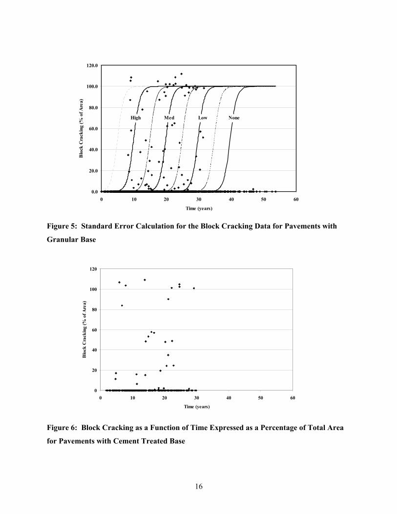
16

Figure 5: Standard Error Calculation for the Block Cracking Data for Pavements with

Granular Base


for Pavements with Cement Treated Base

0.0

20.0

40.0

60.0

80.0

100.0

120.0

0 10 20 30 40 50 60

Time (years)

Blo

ck C

rack

ing

(% o

f Are

a)

High None Low Med

0

20

40

60

80

100

120

0 10 20 30 40 50 60

Time (years)

Blo

ck C

rack

ing

(% o

f Are

a)

17

Figure 7: General Trends of Block Cracking as a Function of Time for Flexible Pavements

with CTB Expressed as a Percentage of Total Area for Pavements

Figure 8: Block Cracking Prediction Curves for Pavements with Cement Treated Base

0

20

40

60

80

100

120

0 10 20 30 40 50 60

Time (years)

Blo

ck C

rack

ing

(% o

f Are

a)

High Med Low None

0

20

40

60

80

100

120

0 10 20 30 40 50 60

Time (years)

Blo

ck C

rack

ing

(% o

f Are

a)

18

Figure 9: Sealed Longitudinal Cracking (NWP) as a Function of Time

Figure 10: Longitudinal Cracking Trends with CTB Base for New Flexible Pavements

0

500

1000

1500

2000

2500

0 10 20 30 40 50 60 70 80 90

Time (years)

Seal

ed L

ongi

tudi

nal C

rack

ing,

NW

P (m

/km

)

High NoneLowMed

0

500

1000

1500

2000

2500

0 10 20 30 40 50 60

Time (years)

Long

itudi

nal C

rack

ing

NW

P (m

/km

)

19

Figure 11: Longitudinal Cracking (NWP) as a Function of Time with CTB for New

Flexible Pavement

Figure 12: Longitudinal Cracking Function of Time for HMA Overlays

0

500

1000

1500

2000

2500

0 10 20 30 40 50 60

Time (years)

Long

itudi

nal C

rack

ing

NWP

(m/k

m)

High NoneLowMed

0

500

1000

1500

2000

2500

0 5 10 15 20 25 30 35 40

Time (years)

Seal

ed L

ongi

tudi

nal C

rack

ing

WP

(m/k

m)

High NoneLowMed

20

Figure 13: Patching Trends for New Flexible Pavements

Figure 14: Patching Trends for HMA Overlays

0

5

10

15

20

25

0 10 20 30 40 50 60

Time (years)

Path

ing

(% o

f Are

a)

High NoneLowMed

0

5

10

15

20

25

0 10 20 30 40 50 60

Time (years)

Patc

hing

(% o

f Are

a)

HighNone

Low

Med

21

Figure 15: Potholes Trends for HMA Overlays

0.00

0.02

0.04

0.06

0.08

0.10

0.12

0 5 10 15 20 25 30

Time (years)

Poth

oles

(% o

f Are

a)

High NoneLowMed

background and preliminary smoothness prediction...

Documents