bachelor thesis in computer science · bachelor thesis in computer science development of a data...

Eberhard Karls Universität TübingenMathematisch-Naturwissenschaftliche Fakultät

Wilhelm-Schickard-Institut für Informatik

Bachelor Thesis in Computer Science

Development of a Data Provenance AnalysisTool for Python Bytecode

Nadejda Ismailova

1 Mai 2015

Reviewer

Prof. Dr. Torsten GrustDatabase Systems Research Group

University of Tübingen

Supervisor

Tobias MüllerDatabase Systems Research Group

University of Tübingen

Ismailova NadejdaDevelopment of a Data Provenance Analysis Toolfor Python BytecodeBachelor Thesis in Computer ScienceEberhard Karls Universität TübingenPeriod: 01.01.2015 - 01.05.2015

AbstractData Provenance describes the origins of data. In this thesis we propose anapproach of computing data provenance when data of interest is created bya Python program and present a tool implementing this approach. In imple-menting the tool, we adopt the following idea. In the first step, the programis instrumented to log data. In the second step, the code is analyzed withrespect to the logged data and provenance information is computed. A novelaspect of this work is instrumentation and analysis of the bytecode of the givenPython program with the aim of computing data provenance.

i

Contents

1 Introduction 1

2 Data Provenance 32.1 Notion of Data Provenance . . . . . . . . . . . . . . . . . . . . . 4

2.1.1 Why, How and Where . . . . . . . . . . . . . . . . . . . 42.1.2 Example . . . . . . . . . . . . . . . . . . . . . . . . . . . 5

2.2 Program Slicing and Dependency Provenance . . . . . . . . . . 72.2.1 Program Slicing . . . . . . . . . . . . . . . . . . . . . . . 72.2.2 Dependency Provenance . . . . . . . . . . . . . . . . . . 102.2.3 Example . . . . . . . . . . . . . . . . . . . . . . . . . . . 112.2.4 Limits of the model . . . . . . . . . . . . . . . . . . . . . 11

2.3 Provenance in Python Programs . . . . . . . . . . . . . . . . . . 122.3.1 Dependencies . . . . . . . . . . . . . . . . . . . . . . . . 122.3.2 AA, AR, RA, RR Dependencies . . . . . . . . . . . . . . 14

3 The Algorithm 193.1 General Approach . . . . . . . . . . . . . . . . . . . . . . . . . . 203.2 Instrumentation . . . . . . . . . . . . . . . . . . . . . . . . . . . 21

3.2.1 Execution . . . . . . . . . . . . . . . . . . . . . . . . . . 233.3 Dependency Analysis . . . . . . . . . . . . . . . . . . . . . . . . 233.4 Python Bytecode Approach . . . . . . . . . . . . . . . . . . . . 24

4 Python Bytecode 254.1 CPython . . . . . . . . . . . . . . . . . . . . . . . . . . . . . . . 264.2 Program Execution in Python . . . . . . . . . . . . . . . . . . . 264.3 Bytecode . . . . . . . . . . . . . . . . . . . . . . . . . . . . . . . 26

iii

Contents

4.4 Program Code Modification . . . . . . . . . . . . . . . . . . . . 294.4.1 Python Code Objects . . . . . . . . . . . . . . . . . . . . 294.4.2 Nested Code Objects . . . . . . . . . . . . . . . . . . . . 304.4.3 Byteplay . . . . . . . . . . . . . . . . . . . . . . . . . . . 324.4.4 Modifying Bytecode . . . . . . . . . . . . . . . . . . . . 33

5 Implementation 355.1 Application Overview . . . . . . . . . . . . . . . . . . . . . . . . 36

5.1.1 Program Interface . . . . . . . . . . . . . . . . . . . . . . 375.2 Instrumentation . . . . . . . . . . . . . . . . . . . . . . . . . . . 38

5.2.1 Logger . . . . . . . . . . . . . . . . . . . . . . . . . . . . 395.2.2 Bytecode Instrumentation . . . . . . . . . . . . . . . . . 405.2.3 What has to be logged . . . . . . . . . . . . . . . . . . . 435.2.4 Database as Log . . . . . . . . . . . . . . . . . . . . . . 54

5.3 Dependency Analysis . . . . . . . . . . . . . . . . . . . . . . . . 575.3.1 Interpreter Concept . . . . . . . . . . . . . . . . . . . . . 595.3.2 Provenance Representation . . . . . . . . . . . . . . . . . 605.3.3 Dependency Stack . . . . . . . . . . . . . . . . . . . . . 645.3.4 Handling Opcodes . . . . . . . . . . . . . . . . . . . . . 665.3.5 Filtering Out Argument and Return Values Dependencies 665.3.6 Storing Dependencies in DB . . . . . . . . . . . . . . . . 67

5.4 Notes . . . . . . . . . . . . . . . . . . . . . . . . . . . . . . . . . 685.4.1 Input Restrictions . . . . . . . . . . . . . . . . . . . . . . 685.4.2 Excluded source code structures . . . . . . . . . . . . . . 685.4.3 CPython Bytecode . . . . . . . . . . . . . . . . . . . . . 69

6 Conclusion and Outlook 716.1 Conclusion . . . . . . . . . . . . . . . . . . . . . . . . . . . . . . 716.2 Future Work . . . . . . . . . . . . . . . . . . . . . . . . . . . . . 71

List of Figures 74

Listings 77

List of Abbreviations 79

iv

Contents

References 81

v

1 IntroductionData provenance provides historical and contextual information about thesource of the data of interest and the way it was produced. This generalconcept was studied in and applied to many different contexts and use cases,such as business applications, the Web, distributed systems, databases andmany others. In databases, why, where [CCT09] and dependence [CAA07]provenance notions have been proposed, which explain the output data of aquery in terms of the input data. We will focus on these provenance notions.In this thesis, we develop a tool for computing data provenance in a Pythonprogram. The tool will be a part of a workflow for visualizing provenance of agiven SQL query. Figure 1.1 illustrates the workflow(the right branch).

Figure 1.1: Project context

In the workflow, the SQL query of interest is translated to a Python program.The SQL Compiler doing that is still in development.As next, data provenance is computed through analysis of the generated

1

1 Introduction

Python program. Currently, this task is done by the AST Data ProvenanceAnalysis Tool, which works on the Abstract Syntax Tree representation of theprogram. In this work we develop an alternative Bytecode Data ProvenanceAnalysis Tool, which will derive provenance by processing the bytecode of thegiven program.Finally, analysis results can be visualized in a web-based Data ProvenanceVisualisation Tool proposed by [Bet14].The tool proposed here is computing provenance in two steps. Instrumentationof the bytecode, so that additional information is logged at run time, is thethe first step. Symbolic execution, which derives dependencies between inputand output data, is the second step.The document structure is as follows.In Chapters 2 - 4 we provide required background information and the basictechniques needed for the implementation. Here, Chapter 2 introduces dataprovenance notions and a possible interpretation of it in terms of Python pro-grams. Chapter 3 presents the general algorithm for computing provenance inprogram context. Finally, Chapter 4 gives an overview of the Python compi-lation process and shows what bytecode instrumentation is.Chapter 5 is devoted to the implementation.At last, we give our conclusions and propose some issues for the future workin Chapter 6.The implementation of the tool is leant on the existing AST implementa-tion and have the same input and output interfaces. For this reason, severalmodules (e.g. for database communication) of the AST-Implementation wereadapted for use in the current implementation.Screenshots of the visualisation [Bet14] are used throughout the work.

2

2 Data Provenance

Chapter OutlineThe structure of this chapter is as follows.In Sections 2.1 and 2.2 we first introduce the notion of data provenance. Wethen provide an overview of the different kinds of data provenance and de-scribe them with the help of an example. Finally, we propose how the dataprovenance notions mentioned can be understood in terms of a given Pythonprogram and transfer the data provenance concept to dependencies betweenargument and return values.In Section 2.3 we show the different perspectives of the dependencies betweenprogram arguments and program’s return value(s), which are eventually theoutput of the analysis tool.

3

2 Data Provenance

2.1 Notion of Data ProvenanceData provenance (also called lineage) records the source (where does the pieceof data come from), derivation (the process by which the piece of data wasproduced), or other historical and contextual information about the data. Wecan find many forms of it in our daily life. For instance, a simple and familiarexample is the time-date and ownership information of the files in the filesystems.Such information can be useful in numberless applications and contexts. Ac-cordingly, the topic has been the focus of many research projects and prototypesystems in many different areas. However in this work we focus on the notionsof provenance as described in the context of databases [BKWC01], [CCT09],[CWW00] .

2.1.1 Why, How and WhereIn the databases context provenance has been studied inter alia from threeperspectives, that, intuitively, describe following relationships between theinput and the output data sets 1:

• Where Provenance: where does a piece of output data set come from theinput data set? In other words, where-provenance points to the locationin the input, where the output values were copied from.• Why Provenance: why is a piece of data in the output data set? Thus,

why-provenance refers to input values which influence the occurrence ofdata of interest in the output.• How Provenance: how was a piece of output data set produced in detail?

Our interpretation of where provenance is extended to include not only loca-tions of copied values, but all input parts participating in computation of therelevant output value.Whereas we discuss why and where provenance at some points in the nextchapters, how provenance is not considered in the rest of the thesis.

1For more detailed and/or formal description see [BKWC01], [CCT09].

4

2.1 Notion of Data Provenance

2.1.2 Example

We will illustrate the idea of why and where provenance through an examplefrom [CCT09]. Consider the following query:

Listing 2.1: Example query

1 SELECT a.name, a.phone2 FROM Agencies a, ExternalTours e3 WHERE a.name = e.name AND e.type="boat"

Suppose that the query is executed on tables agencies and externalToursas in Figure 2.1, where the labels a1, . . . , r3 are used to identify the records.In the figure why provenance is highlighted orange and where provenance ishighlighted yellow.The results of the query are shown in the table result. As we can see, thequery returns names and phone numbers of all agencies offering boat tours.If we did not expect the “HarborCruz” to be an agency offering boat tours,we could ask ourselves why it is in the output. To get the answer, we look atthe why provenance of this record. In Figure 2.1 it is highlighted orange (inthis case the field has the same why provenance as the record containing it).We see that the field r3.phone is included in the result because a2.name, t5.name

and t5.type values, which are relevant for the join and filtering conditions ofthe query, qualify that record to be returned in the output.Now we might like to know, where the field r3.phone is coming from. For in-stance, when the number is not correct, we would like to fix it in the sourcetable. In such cases where provenance provides the information we need. Fig-ure 2.1 shows that the field in the result is copied from a2.phone field in agen-cies.

Figure 2.1: Why and where provenance

5

2 Data Provenance

Note that the result contains duplicate entries. A reasonable question at thispoint might be: why does the “BayTours” entry occur twice in the output?For those who wonder, our query semantics is not eliminating duplicates fromthe output. We use this fact to show that with the help of provenance (whyprovenance in this case) we can explain why there are duplicates in the resultin a very simple way. A name of an agency and a tour type do not identifya single row in the join table externalTours since there are boat tours todifferent destinations, that is why we get the “Bay Tours” entry twice. Andthat is exactly what we see in the figure shown below. In Figure 2.2 it is easyto see that the existence of each of duplicate rows in the output is justified bya different row in the input externalTours table.

Figure 2.2: Duplicate entries have different provenance values

The presented example is simple, but if we consider that the most real-worlddatabases have hundreds of columns and millions of rows, than an explanationto the relationships between each part of input and output seems correspond-ingly useful and important.

6

2.2 Program Slicing and Dependency Provenance

2.2 Program Slicing and Dependency ProvenanceA more general perspective on data provenance was also introduced [CAA07].To understand it, we start with a few words about program slicing.

2.2.1 Program Slicing

Program slicing [Wei81] is a form of program analysis that identifies programparts which contributed to program results, primarily for debugging purposes.As in other program analysis techniques dependence is a key concept in slic-ing [ABHR99], describing how variables or control flow points influence otherprogram parts.• A slice to some variable a consists of all program statements that some-

how affect the value of a, or, in other words, on which variable a depends.Naturally, we want slices to be as small and thus easy to understand as possible,so the program itself as a trivial slice is not of interest.In cases where program has conditional expressions, we differentiate betweenstatic and dynamic slices. In case of a static slice we don’t know which branchwas taken at run time and so consider instructions and dependencies in bothbranches. In contrast, dynamic slices only contain statements from the actuallyexecuted branch, statements and dependencies in branches that were not takenare ignored.As an example, suppose a program as in Listing 2.2:

Listing 2.2: Function takes a list of numbers as input and returns a list wherenumbers are reordered in a way that even numbers come first in the list.

1 def sortOnEvenNumbers(numbers):2

3 numElements = len(numbers)4 # index for even numbers5 evenIndex = -16 # index for odd numbers7 oddIndex = numElements8 # result list, initialized with zeros9 sortedList = [0] * numElements

10

11 # index variable for iteration over the input list12 i = 013 while i < numElements:14 # read next list’s element15 n = numbers[i]16 # got an even number17 if n % 2 == 0:18 # fill list from the left19 evenIndex += 1

7

2 Data Provenance

20 sortedList[evenIndex] = n21 # got an odd number22 else:23 # fill list from the right24 oddIndex -= 125 sortedList[oddIndex] = n26 i = i+127

28 print sortedList29

30 # input31 numbersList = [1,2,3,4,5,6,7,8,9,10]32 # function call:33 sortOnEvenNumbers(numbersList)34

35 # output:36 # [2, 4, 6, 8, 10, 9, 7, 5, 3, 1]

The program just moves even numbers in a given list to be at the beginningof the list and odd numbers to come afterwards.Following Listings give examples of static and dynamic slices to different vari-ables of the function in Listing 2.2. Statements not included in a slice areshown grayed.

Listing 2.3: Slice with respect to index variable i

1 numElements = len(numbers)2 evenIndex = -13 oddIndex = numElements4 sortedList = [0] * numElements5

6 i = 07 while i < numElements:8 n = numbers[i]9 if n % 2 == 0:

10 evenIndex += 111 sortedList[evenIndex] = n12 else:13 oddIndex -= 114 sortedList[oddIndex] = n15 i = i+116

17 print sortedList

Listing 2.4: Static slice with respect to sortedList

1 numElements = len(numbers)2 evenIndex = -13 oddIndex = numElements4 sortedList = [0] * numElements

8


5



17 print sortedList

Listing 2.5: Dynamic slice with respect tosortedList with i = 2, i.e. n = 3




17 print sortedList

Listing 2.6: Dynamic slice with respect tosortedList with i = 5, i.e. n = 6




17 print sortedList

Static slice to sortedList omits only the print sortedList statement at theend of the program, since it is the only statement not influencing sortedList.But dynamic slices are a bit more simplified, because according to conditionevaluation in the if clause only one branch affects the value of sortedListand another branch is omitted.

9

2 Data Provenance

2.2.2 Dependency ProvenanceAs we know by now, provenance explains the results of a query in terms ofthe input data. Intuitively, we say that the input has contributed to or hasinfluenced or is relevant to the output. Cheney et al. generalize that intuitionby defining dependence between output and input if a change on the inputmay result in a change to the output [CAA07].Here we see an outstanding similarity between program slicing and data prove-nance. In program slicing as well as in data provenance we are looking for partscontributing to the output, with the difference that provenance identify partsin the input database and slicing in the program. The analogy is more detaileddiscussed in [Che07].Similar to dependence concept in slicing dependence provenance is defined,formal details to which were proposed by [CAA07]. Intuitively,

• Dependency provenance is information relating each part of the outputof a query to a set of parts of the input on which the output partdepends [Che07].

As an example, consider an output record r with a field A and an input record scontaining field B. Due to the definition above, r.A depends on s.B if changings.B in some way either removes record r from the output completely or changesthe value of r.A. The dependency provenance of r.A is then the set of all suchinput fields s.* on which r.A depends.The following notation is used throughout the thesis. For some value A whichdepends on B we write the dependency as a tuple (A,B). For some value Adepending on several values B,C,D, ... a dependency provenance set is givenas {B, C, D, . . .} to list all the dependencies.Additionally, whenever the phrase “dependency-correctness” is used in the restof this thesis, we intend that the provenance set computed for some outputvalue contains all parts of the input which may lead to a change of the outputvalue (compare [CAA07]).

10


2.2.3 ExampleFor convenience we are going back to our example from Section 2.1.2.For ease of presentation in all the following figures same ( orange ) highlightingis used for all dependency provenance items.

Figure 2.3: Dependency provenance of r3.phone

The dependency provenance of the result field r3.phone is the set{ a2.name, t5.name, t5.type, a2.phone }, since changing these values can affectthe result. In more detail: r3.phone is copied from a2.phone, so changing a2.phone

would change r3.phone. Fields a2.name, t5.name are participating in the join andt5.type in the filtering condition, that is changing these values can exclude r3

from the output.Dually, r3.phone does not depend on all the other fields, what means, that afterany modifications on these fields the r3.phone value of the “HarborCruz” entrywould be still the same and would still be part of the output.

2.2.4 Limits of the modelCheney et al.[CAA07] showed that obtaining “minimal” dependence informa-tion is undecidable. So our goal is to approximate the dependency-correctprovenance minimum for each of the output items.

11

2 Data Provenance

2.3 Provenance in Python ProgramsAlthough the where and why provenance can be interpreted and representedin terms of Python programs, the concept proposed here is based on the ideaof dependency provenance. We yet tried to keep the architecture adaptablefor why and where differentiation in the future.Speaking about provenance in a program, dependencies within a single Pythonmodule are meant, thus inter-module dependencies are not analyzed.

2.3.1 DependenciesAll the provenance definitions from above stay the same in terms of Pythonprograms, with the difference that we no longer consider fields or records orrelations. Instead we concentrate on variables (their values more precisely),what in effect is more general, since the value a variable points to can representa single field or a single record(row) or the whole relation(table). Note thatdependence sets are still derived for data, i.e. values variables are pointingto. So if at some point in the program a variable is re-bound and thereafterpoints to another value, then a different dependence set is associated withthe variable, namely, the dependence set of the value currently bound to thevariable name.If a variable is pointing to some kind of collection (tuple, list, dictionary),then we derive dependencies for each of the elements in the collection. In theremainder of the work an element of a collection is identified by its “path”, seeListing 2.7.

Listing 2.7: Identifying collection items through their paths

1 # Suppose a list of dictionaries:2 list = [{"key1": 1}, {"key2": 2}, {"key3": 3}, {"key4": 4}]3 # In Python we read the value 2 as follows:4 theTwo = list[1]["key2"]5 # The path to the value 2 is: [’list’, ’1’, ’key2’]6 # The same for the value 4: [’list’, ’3’, ’key4’]

Since provenance explains output in terms of input, dependence set of thereturn value (and dependence sets of all collection elements if a collection isreturned) is what we are aiming for.Consider the following Python program:

Listing 2.8: Dependencies in a Python Program

1 def sumUpMultiples(numbers, factor):2 sum = 03 i = 04 numRows = len(numbers)

12

https://docs.python.org/2/tutorial/modules.html

https://docs.python.org/2.7/reference/executionmodel.html#naming-and-binding

2.3 Provenance in Python Programs

5 while i < numRows:6 n = numbers[i]7 # filtering condition:8 # here the decision is made,9 # whether an element of the input list

10 # will contribute to the output value11 # <-> why provenance12 if n % factor == 0:13 # input list’s element n is14 # added to the return value sum15 # <-> where provenance16 sum += n17 i = i+118

19 return sum20

21 numbers = [1, 2, 3, 4, 5, 6, 7, 8, 9, 10]22 print sumUpMultiples(numbers, 3)23

24 # output:25 # 18 <-> 3 + 6 + 9

The function takes a list of numbers and a factor. It returns the sum of allnumbers in the list, which are multiples of factor.With the given input the function computes the sum of all the multiples ofthree in the number sequence 1 - 10, that is 3 + 6 + 9 = 18.How is the sum computed? Well, we iterate over the numbers list, checkwhether a number is a multiple of the factor variable’s value and add itto the sum variable if it is. So what we return is computed from a set of in-put list items and the factor decides which items these are. Hence, the sum

depends on those list items, which contributed to its value, and on factor,which decides which items to involve into computation.For our example input this means: the returned 18 depends on values{3,6,9,3}. Both 3 entries are required, because they are indeed two dif-ferent entities: one is the input item from the numbers list and the secondis the value of the factor variable. Thus, the dependence provenance set ofthe sum variable is {[’numbers’, ’2’], [’numbers’, ’5’], [’numbers’, ’

8’], factor}.There are two significant points in the program influencing sum variable’sprovenance.On one hand, the if clause in line 12 is filtering list items to multiples offactor. If one would ask ‘why is 9 added to sum ?’ the answer would be‘Because 9 is a multiple of 3’. That is, for an n that satisfies the condition,values of both n and factor are representing the why provenance of sum.On the other hand, the sum += n statement, which is actually computing the

13

2 Data Provenance

output from the input. According to our interpretation of provenance, what-ever n is pointing to in the moment of execution is part of the where provenanceof sum.In other words, an interesting and reasonable interpretation is to describe whyprovenance in a program by control dependencies and where provenance bydata dependencies.The program analyzed here only contains one function call. However, a pro-gram in general can generate output by modifying the original input datathrough several sequential calls to different functions or nested calls withinone function. The handling of dependencies in this context is discussed in thenext section.

2.3.2 AA, AR, RA, RR Dependencies

In the last section an interpretation of dependence provenance in a Pythonprogram was proposed, where a single function call computed the output. Morecomplex programs involve several steps, i.e. multiple sequential function calls.Furthermore, since the tool is supposed to analyze translated SQL queries, itseems eligible to assume, that nested queries will occur, which probably wouldbe translated to nested function calls.In such cases we still want to trace the final program output back to the originalprogram input. But, additionally, the intermediate results, i.e return valuesof all the called functions, should be kept and explained in terms of the inputof the particular function too, as well as the data flow between single functioncalls 2.In this context, following four perspectives of dependency relationship betweeninput, i.e. function arguments, and output, i.e. function return value, areproposed:

• RA - Return value on Arguments dependence:(return value, argument)They describe how the return value of a function depends on the argu-ments of the same function. This is the base case we saw in Section 2.3.1.• AR - Arguments on Return values dependence:

(argument, return value)When an argument of a currently executed function somehow dependson a return value of some other previously called function, we call it anAR dependency.

2Talking about functions here and in the rest of the thesis, Python’s user defined functionsare meant, see “Callable types” in the Python Documentation [Fou13a].

14

http://en.wikipedia.org/wiki/Data_dependency#Control_Dependency

http://en.wikipedia.org/wiki/Data_dependency


• AA - Arguments on Arguments dependence:(argument, argument)This kind of dependencies form when a nested function call occurs andthe arguments of the called function somehow depend on the argumentsof the caller.• RR - Return value on Return value dependence:

(return value, return value)Again, this kind of dependencies form when a nested function calloccurs. Here, the return value of the caller depends on the return valueof the called function.

These dependencies are the output of the tool developed in this thesis.Observe that only for RA dependencies both parts of the relationship, returnvalue and argument, belong to the same namespace. In the remaining caseselements from at least two different namespaces are somehow interacting.Here, it is important to know, that we describe the relationship always from theperspective of the current namespace, i.e. namespace currently being analyzed:(value in current namespace, value in a different namespace).Note also that all four kinds of dependencies imply both why and where prove-nance, thus we have AA why and where provenance, AR why and where prove-nance, RA why and where provenance, RR why and where provenance.In the remainder of the thesis, the (sub)set of all dependencies in a program isnoted as {(v1, v2), (v2, v3), (v4, v5), . . .}, where (v1, v2) is one of dependenciesdefined above between values v1 and v2.As mentioned, we have illustrated RA dependencies in the program in Sec-tion 2.3.1 already. Following examples make the idea of the remained AR,AA, RR dependencies clear.

Sequential calls

AR dependencies occur, when a return value of a function influence whicharguments another function called later will get. Look at the Figure 2.4:In the figure, three functions are called sequentially. The different namespacesare illustrated as grayed boxes.The firstPassThrough function gets a list [1, 2, 3, 4] as input. Obviously,it just forwards the input to the output. The blue arrows illustrate the RAdependencies.The next function call filter() takes the return value res1 of the previousfunction as an argument. Thus, this argument depends on the return valueof the other function. The red arrows represent these AR dependencies: thefirst list item of the input list of filter() depends on the first list item of

15

https://docs.python.org/2/tutorial/classes.html#python-scopes-and-namespaces

2 Data Provenance

Figure 2.4: RA and AR dependencies

the output list of firstPassThrough() - (1,1), the second list item of theinput list of filter() depends on the second list item of the output list offirstPassThrough() - (2,2), and so on: (3,3), (4,4).The filter() function returns only items from the input list, which are< 3, i.e [1, 2]. This return value is then passed as argument to thesecondPassThrough() function, that is, we have AR dependencies again. In-put of the secondPassThrough() depends on the output of the filter():{(1,1),(2,2)}.The secondPassThrough() only returns its own input, again.Now, when we look at the 1 at the very end, returned by secondPassThrough

(), and follow the arrows representing the AR and RA dependencies, we cometo the very first 1 defined in the list. By this means, we tracked all thetransformations the output value 1 was processed by back to its origin.

Nested calls

AA and RR dependencies occur, when a function has recursive calls or calls tosome other functions within its body. The Figure 2.5 below shows one possiblescenario.Two functions passThrough() and filter() are called sequentially. How-ever, now filter() calls to another function nestedFunctionCall() inside

16


its body. Thereby, nestedFunctionCall() takes input of the filter() asown input, these are AA dependencies shown by green arrows. The output ofthe nestedFunctionCall() is returned by filter() as own output, which isshown by the orange RR dependencies arrows.

Figure 2.5: RA and AR dependencies

Again, at the end each of the [1, 2] output items can be tracked to its originby following the dependency arrows.

17

3 The Algorithm

Chapter OutlineIn this Chapter the algorithm how to derive dependence provenance for a givenprogram is proposed.The first section describes the general procedure and gives an overview of thecomponents.In the rest of the Chapter we take a closer look at the instrumentation andthe dependency analysis steps.

19

3 The Algorithm

3.1 General ApproachIn this thesis, provenance is computed through value-less or symbolic execu-tion of the input program. Here, execution means, that while evaluating theprogram, we follow the same control flow and access the same subscript el-ements, as it would be done at run time. Value-less means that we do notinvolve the actual values into computation, which were given by the input ordefined by the program. Instead, dependencies are “assigned” to the variablesand the data processing steps in the program are interpreted in terms of thesedependencies. The output produced this way contains the provenance of theoutput value produced by the real execution.Yet, before we can start that simulated “execution”, we need to know thefollowing:• control flow decisions, i.e. whether an if-block or a loop body was exe-

cuted• collection access, i.e. subscripts used to read or write collection items,

for example, value of the index variable i when accessing someArray[i]

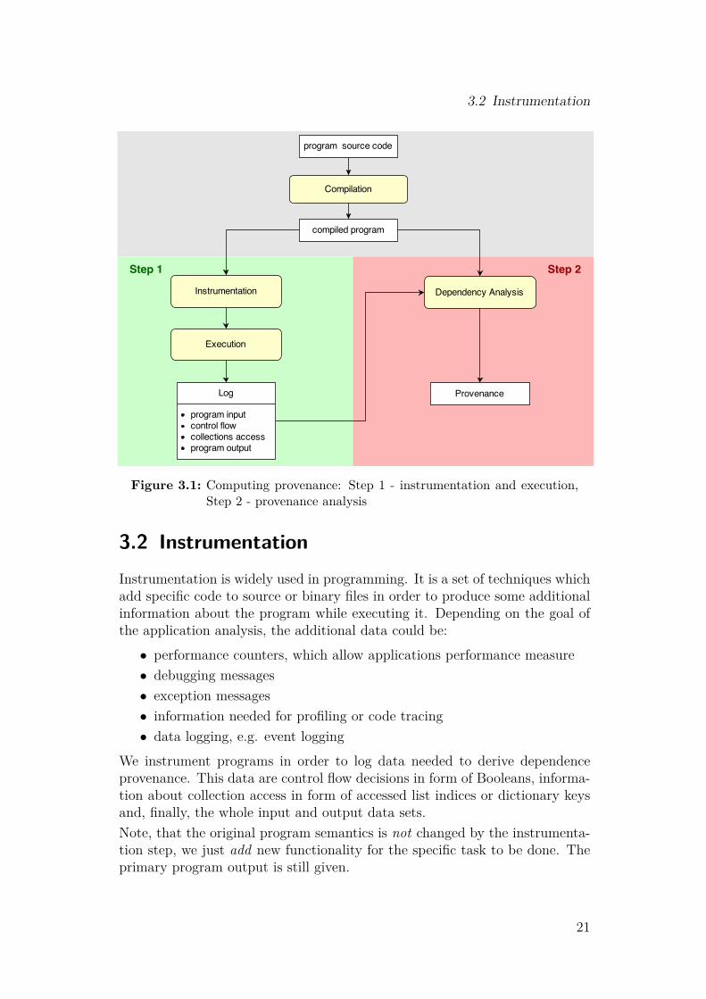
To get this information, we have to actually run the program with the inputdata of interest and somehow remember relevant data.Therefore, the whole procedure is split up into two steps, see Figure 3.1.We get the program to analyze as input.In the first step, illustrated in the green area of the diagram, we log run timedata. This is done as follows. First, we instrument the input program, i.e.extend it with additional functionality. Then we run the program, and at theexecution time the modified part of the program writes the run time informa-tion we need into the Log.The second step represents the value-less execution. Here, dependencies areanalyzed with the help of Log data and, as a result, provenance of the programoutput is computed.In the next sections, instrumentation and dependency analysis components aredescribed in more detail.The provenance analysis approach proposed here seems to be similar to theeager(book-keeping) approach of computing provenance [CCT09], but a de-tailed comparison is required, which, unfortunately, would go beyond the scopeof the thesis.

20

3.2 Instrumentation

Figure 3.1: Computing provenance: Step 1 - instrumentation and execution,Step 2 - provenance analysis

3.2 InstrumentationInstrumentation is widely used in programming. It is a set of techniques whichadd specific code to source or binary files in order to produce some additionalinformation about the program while executing it. Depending on the goal ofthe application analysis, the additional data could be:• performance counters, which allow applications performance measure• debugging messages• exception messages• information needed for profiling or code tracing• data logging, e.g. event logging

We instrument programs in order to log data needed to derive dependenceprovenance. This data are control flow decisions in form of Booleans, informa-tion about collection access in form of accessed list indices or dictionary keysand, finally, the whole input and output data sets.Note, that the original program semantics is not changed by the instrumenta-tion step, we just add new functionality for the specific task to be done. Theprimary program output is still given.

21

3 The Algorithm

The input and the output are logged, because the goal is to derive provenancefor the output and, in this manner, explain it in terms of the input.The control flow and the subscripts logs are central, since in the analysis stepwe want to reproduce the program flow at the execution time. Both are rep-resented by a chronological stream of Boolean or subscript values respectively.To illustrate this, a pseudocode example is shown in Listing 3.1

Listing 3.1: Control flow and subscripts Log

1 list = [1, 2, 3, 4] # a list containing 4 numbers2 length = len(list)3 i = 0 # index variable4 while i < length: # ctrl flow log: execute loop body? true/

false5 number = list[i] # subscripts log: value of i?6 i += 17 if number % 2 == 0 # ctrl flow log: execute if block? true/

false8 print "even"9 else:

10 print "odd"11

12 # output: odd, even, odd, even13

14 # iteration Log state (true = t, false = f)15 # 1 ctrl flow: [t, f,]16 # subscripts: [0,]17 # 2 ctrl flow: [t, f, t, t,]18 # subscripts: [0, 1, ]19 # 3 ctrl flow: [t, f, t, t, t, f,]20 # subscripts: [0, 1, 2,]21 # 4(last) ctrl flow: [t, f, t, t, t, f, t, t,]22 # subscripts: [0, 1, 2, 3]23 #24 # The next while condition evaluation says "false",25 # i.e. ’loop body is not executed’ decision is logged:26 # ctrl flow: [t, f, t, t, t, f, t, t, f]27 #28 # Log state after execution finished:29 # ctrl flow: [t, f, t, t, t, f, t, t, f]30 # subscripts: [0, 1, 2, 3]

A list of four numbers is iterated and for each item "even" is printed if thevalue is even and "odd" is printed if the value is odd.In the execution order the ctrl flow log is updated with the boolean values,which while(line 4) or if(line 7) conditions respectively were evaluated to. Inthe first iteration, while condition was satisfied, so the first entry in the logis true. In contrast, the if condition was not satisfied, because 1 is not even.Thus, the second entry in the log is false. The state of the log after each

22

3.3 Dependency Analysis

iteration is shown in lines 12-20.Due to the reading of list items in line 5 the value of the index variablei is appended to the subscripts log. Its state after each iteration is given too.

Summing up, in the instrumentation step we extend a given program withadditional instructions, so that input, output, control flow and collection accessdata are written to a Log when the program is executed.

3.2.1 ExecutionInstrumentation itself just extends the program. After the instrumentationthe modified program has to be run. Original as well as added functionalityis then executed, producing the output primarily meant in the program and,at the same time, specific output coming from the instrumented parts of theprogram, which is in our case the Log data.

3.3 Dependency AnalysisIn the second step we derive dependence provenance through symbolic execu-tion of the original program.Symbolic execution is an analysis technique, which is not working with actualvariable values but assigns symbols as variable’s value instead. We adapt thisconcept to our needs by assigning provenance sets and not symbols.The program is analyzed in a static way, that is we are not actually executingit, but follow the program flow as it would be executed if we would run it.Each value has a dependency set associated with it. When some computationsare done on the values we add or remove dependencies to or from the setaccording to the semantics of the computation. In this manner, after we haveanalyzed the whole program, dependence provenance set of the output valuesis computed.When a control flow decision has to be made, i.e in a loop or in if-else blocks, wedon’t consider several possible flows, but check the condition’s boolean valuewe have logged in the previous step and interpret only the branch which wasreally executed at run time. Consequently, the result dependence set includesonly dependencies that actually contributed to the output and does not containdependencies from program parts, which were not processed. In other words,for a value we only consider dependencies present in a dynamic slice of theprogram on that value.Collection access is interpreted in the same way. We look up the index toaccess in our log-tables in the database and then work with the dependencyprovenance set associated with the collection’s element at that index.

23

3 The Algorithm

3.4 Python Bytecode ApproachThis tool is supposed to get Python programs as input. Thus, the instrumen-tation and the analysis steps of the algorithm have to be applied to Pythonprograms. Program analysis in general provides many techniques, some work-ing on source code and some with binary files. In this work, we are going toinstrument and analyze compiled Python code, the bytecode.

24

4 Python Bytecode

Chapter OutlineIn this chapter we explain what bytecode, a structure Python programs arecompiled to, looks like. It is more a vertical slice through the material, sincethe compilation process and Python language internals is a large topic. We willlearn what Python code objects are and how we get a code object associatedwith a module or a function. Finally, we will acquaint ourself with modificationof bytecode and investigate, what the bytecode representation of some codeconstructs looks like.

25

4 Python Bytecode

4.1 CPythonThere are several alternate implementations of Python. In this work, whereverwe say “Python” the CPython implementation is meant. CPython is the orig-inal and most-maintained implementation of Python, written in C [Fou13b].All code in this thesis was written in and tested against Python 2.7.5. Further-more, since other (compiler) versions could translate same source code state-ments and constructs to different bytecode representations and structures, theinput programs are restricted to use of bytecode instructions as implementedfor Python 2.7.5. The latter are described in the Documentation of the dis

module.

4.2 Program Execution in PythonSimilar to Java, Python does not translate source code to machine code di-rectly, but compiles it to an intermediate result first, bytecode. It is storedand can be accessed as a .pyc file. After compilation Python’s Virtual Machineexecutes the produced bytecode [Fou15].The compilation chain is illustrated in the next figure:

Figure 4.1: Program execution in Python

In its concept Python interpreter is similar to the microprocessor. When ex-ecuting a program it is processing an instruction stream. This instructionstream is the bytecode, we can think of it as machine code for the PythonVirtual Machine. For managing operands and computation results the inter-preter uses a stack (in comparison to registers in a microprocessor), that iswhy Python Stack Machine is another name for the Python interpreter.The next section shows, how the Stack Machine is working.

4.3 BytecodeWith the help of Python’s dis module we can bring bytecode in a readableform, i.e. disassemble it. Disassembled bytecode looks like microprocessorinstructions. A simple example of a program and its bytecode are shownbelow in the Listings 4.1 and 4.2 respectively. The bytecode of the program isillustrated in the disassembled form mentioned above.

26

https://docs.python.org/2.7/library/dis.html


https://docs.python.org/2.7/glossary.html#term-bytecode

https://docs.python.org/2.7/glossary.html#term-virtual-machine


4.3 Bytecode

Listing 4.1: Simple python program: function returns sum of two arguments

1 def f(a, b):2 res = a + b3 return res

Listing 4.2: Bytecode representation of the function

1 src line address opcode oparg2 -------------------------------------------------------------3 2 0 LOAD_FAST 0 (a)4 3 LOAD_FAST 1 (b)5 6 BINARY_ADD6 7 STORE_FAST 2 (res)7 3 10 LOAD_FAST 2 (res)8 13 RETURN_VALUE

The function’s body consists of two lines. These are represented by the twobytecode blocks in the disassembled output. In src line column in the List-ing 4.2 we see numbers 2 and 3 each introducing the block of instructionsrepresenting the source code line 2 and 3 respectively.In most cases a single line of source code is translated to multiple primitivebytecode instructions. Indeed, from the three lines of code in our exampleprogram six lines bytecode were produced. A simple addition expression inline 2 of our sample code is translated to four bytecode operations: loadingthe first operand, loading the second operand, adding the operands, and finallystoring the result. In general, depending on how complex is the statement totranslate, the corresponding bytecode can become very long.There is some more information in the listing we see as well:• the address of the instruction represents its position in the compiled

code as number of bytes from the beginning of the .pyc file (instructionsare all three bytes long).• the opcode, i.e. operation code name• the oparg, i.e. the operand, which is then resolved to the actual instruc-

tion’s argument, if the instruction requires any parameters. In parenthe-ses we see that resolved argument.

Python Interpreter reads the instructions one by one and produces a re-sult through executing the operation coded in the opcode on the operands.Operands and operation results are stored on an internal stack. The stack isa temporary area, where only references pointing to objects in the heap arestored. While executing an instruction Python interpreter pushes and popsthe references with respect to the opcode. In other words, the interpreter cre-ates and destroys objects in the heap according to the current instruction andpushes or pops the references to these objects to or from the stack.

27

4 Python Bytecode

Figure 4.2 below illustrates what is happening when the bytecode of the pro-gram from above is executed. There TOS means top of the stack, PC meansprogram counter.

Figure 4.2: Bytecode execution

The figure does not explain how the last two instructions are executed. Thelast loading operation puts the reference to the result variable onto the stackagain. Then, the RETURN_VALUE operation returns whatever is on TOS to thecaller.Note that binary operations are working on two operands and are not pro-cessing binary numbers.The full list of opcodes and their meaning and further detailed information tobytecode is described in Python Documentation to bytecode.

28


4.4 Program Code Modification

4.4 Program Code ModificationPython makes it easy to instrument programs, since it is possible to modifycompiled bytecode directly and execute this code afterwards. To understand,how exactly bytecode can be modified, we need to know that Python bytecodeis represented by code objects.

4.4.1 Python Code Objects

In Python everything is an object [Fou13a]. This means, bytecode is an objecttoo. For each module, class, function or an interactively typed command thereis a single code object associated with it and representing its bytecode. Forinstance, for a function we get the code object of the function’s body by readingfunction’s attribute __code__. Code objects have the type “CodeType” andlike the other objects are stored in the heap.In addition to the bytecode itself a code object also stores several attributes,which we do not discuss in detail here and refer to the section describingcode objects of the Python Documentation instead [Fou13a]. At this point weonly put on record that the opargs are resolved by looking up the co_names,co_varnames and co_consts attributes of a code object, which are tuplescontaining the names of global variable names, local variable names (includingfunction arguments) and constants respectively. But even this resolution ineffect invoke checking other code object attributes too, so we do not look atit in detail.

We illustrate this with the sample code from the previous section.

Listing 4.3: Code object attributes: variables and constants

1 def f(a, b):2 res = a + b3 return res4

5 print"co_varnames: " , f.__code__.co_varnames6 print"co_names: " , f.__code__.co_names7 print"co_consts: " , f.__code__.co_consts8

9 Output:10 co_varnames: (’a’, ’b’, ’res’)11 co_names: ()12 co_consts: (None,)

Since no global variables are used the co_names tuple is empty. But if weeconsider a slightly different function as in Listing 4.4, we see that now theglobal variable c is included in the tuple of global variables of the function.

29

4 Python Bytecode

Listing 4.4: Code object attributes: global variables

1 c = 302

3 def f(a, b):4 res = a + b + c5 return res6

7 print"co_varnames: " , f.__code__.co_varnames8 print"co_names: " , f.__code__.co_names9 print"co_consts: " , f.__code__.co_consts

10

11 Output:12 co_varnames: (’a’, ’b’, ’res’)13 co_names: (’c’,)14 co_consts: (None,)

4.4.2 Nested Code ObjectsWhenever a block, which is a piece of Python program text that is executedas a unit, is compiled, a code object is created. Since it is possible to definenested blocks, e.g. a module with a function definition in it, it is also possibleto get nested code objects. Here it is important to know that code objects areimmutable. Therefore, if we want to know whether some code object containsmore code objects, we have to look for entries of the “CodeType” type in itsco_consts tuple.Consider the following code snippet.

Listing 4.5: Simple module code

1 a = 102 b = 203 res = a + b4 print res

Listing 4.6: Variables and constantsof the code

1 co_varnames: ()2 co_names: (’a’, ’b’, ’res’)3 co_consts: (10, 20, None)

We save this piece of code as a file “someModuleExample.py”. From now weconcentrate on cases, where the input Python program is given as .py file, sincethat is the input interface defined in our tool. Getting the input in that waywe have to make use of some Python modules to get the code object associatedwith the program in file, namely py_compile and marshal. Following is thecode getting a code object from a source code file:

Listing 4.7: Code object attributes: global variables

1 # compile the source code, i.e. create the code object andsave it to a .pyc file

2 py_compile.compile("someModuleExample.py")3 # open compiled code

30


https://docs.python.org/2/library/py_compile.html

https://docs.python.org/2/library/marshal.html


4 fd = open("someModuleExample.pyc", ’rb’)5 # first 8 chars of the stream are representing meta data6 magic = fd.read(4) # python version specific magic number7 date = fd.read(4) # compilation date8 # now the code object itself is the next in the stream,9 # load it

10 code_object = marshal.load(fd)11 # reference to the code object in heap is enough, close file12 fd.close()

In Listing 4.6 variables and constants of the loaded code object are shown.Here it is worth pointing out that at module level all variables are global.Accordingly to that co_varnames tuple is empty, as we see. Insofar there areno other points to mention to this code object.Now, suppose we have extracted the addition to a function. For convenience,we also rename the module level variables:

Listing 4.8: Nested code blocks: function definition within a module block

1 def f(a, b):2 res = a + b3 return res4

5 x = 106 y = 207 res = f(x,y)8 print res

This code piece we will save in a different file “someFunctionExample.py”. Weload its code object the same way as above and look at the same attributes:

Listing 4.9: Nested code blocks: function’s code object referenced as constantby the enclosing module code object

1 co_varnames: ()2 co_names: (’f’, ’x’, ’y’, ’res’)3 co_consts: (<code object f at 01FFB608, file

"someFunctionExample.py", line 1>, 10, 20, None)

Whereas the code piece in Listing 4.5 was a single block, here the functiondefinition is an extra block in the module code. We are still observing themodule code object, but now it has the function’s name in its global namestuple and the reference to function’s code object in its constants tuple. Addi-tionally, function code object’s address in the memory and function definition’sposition in the source code are given. If we would define more functions inthis module, more code objects would be listed in the constants tuple of themodule code object.Finally, we present a recursive function, which we can use to explore (nested)code objects structure of any given file:

31

4 Python Bytecode

Listing 4.10: Explore code object’s structure

1 import types2

3 def explore_code_object(co_obj, indent=’’):4 print indent, co_obj.co_name, "(lineno:",

co_obj.co_firstlineno, ")"5 for c in co_obj.co_consts:6 if isinstance(c, types.CodeType):7 explore_code_object(c, indent + ’\t’)8

9 # Applied to "someModuleExample.py":10 <module> (lineno: 1 )11

12 # Applied to "someFunctionExample.py":13 <module> (lineno: 1 )14 f (lineno: 1 )

4.4.3 ByteplayThere are many frameworks for simplified bytecode visualisation and analysis.In this work we use byteplay.

Figure 4.3: Using byteplay for bytecode analysis

Byteplay provides a wrapper object for Python code objects. The bytecode isthen represented by a list of instructions, which in their turn are representedas tuples (opcode, oparg).

32

https://wiki.python.org/moin/ByteplayDoc


4.4.4 Modifying BytecodeThe most interesting code object’s attribute for us is the co_code. It repre-sents the sequence of the code object’s bytecode instructions. Unfortunately,co_code is a read only attribute, so we can not modify it directly. However,for our purposes we don’t need to. In terms of our concept, it is enough toexecute the extended bytecode just once, that is we don’t have to make thechanges persistent. Thus, we just create a new code object, whose co_codeattribute contains a modified copy of the existing instructions sequence of thegiven code object. This new code object can be consequently run and willexecute all the additional effects.

We illustrate the idea on the example from Listing 4.5. The disassembledbytecode of the program looks like what follows:

Listing 4.11: Bytecode of the small sample in Listing 4.5

1 src line address opcode oparg2 -------------------------------------------------------------3 1 0 LOAD_CONST 0 (10) # 10 loaded on TOS4 3 STORE_NAME 0 (a) # 10 stored into a5 # here empty stack again6 2 6 LOAD_CONST 1 (20) # 20 loaded on TOS7 9 STORE_NAME 1 (b) # 20 stored into b8 # here empty stack again9 3 12 LOAD_NAME 0 (a) # a’s value loaded

10 15 LOAD_NAME 1 (b) # b’s value loaded11 18 BINARY_ADD # two values popped, sum on TOS12 19 STORE_NAME 2 (res) # TOS stored into res13 # here empty stack again14 4 22 LOAD_NAME 2 (res) # res’s value on TOS15 25 PRINT_ITEM # TOS popped and printed16 26 PRINT_NEWLINE # line break printed17 27 LOAD_CONST 2 (None) # None on TOS18 30 RETURN_VALUE # TOS returned to the caller

Suppose we want to print a string after a was initialized. For that we add afew instructions (in green) right after the bytecode block of the line 1. In factwe add the same instructions as used at the end of the program, where res isprinted:

33

4 Python Bytecode

Listing 4.12: Modified bytecode

1 src line address opcode oparg2 -------------------------------------------------------------3 1 0 LOAD_CONST 0 (10)4 3 STORE_NAME 0 (a)5 6 LOAD_CONST ’awesome’6 9 PRINT_ITEM7 10 PRINT_NEWLINE8

9 2 11 LOAD_CONST 1 (20)10 14 STORE_NAME 1 (b)11

12 3 17 LOAD_NAME 0 (a)13 20 LOAD_NAME 1 (b)14 23 BINARY_ADD15 24 STORE_NAME 2 (res)16

17 4 27 LOAD_NAME 2 (res)18 30 PRINT_ITEM19 31 PRINT_NEWLINE20 32 LOAD_CONST 2 (None)21 35 RETURN_VALUE

We execute the new created code object and get:

Listing 4.13: Execute modified bytecode

1 exec newCodeObject2

3 # Output:4 awesome5 30

In Python all code objects return something, even if the programmer didn’tdefine any return statements in module’s or function’s code. If no return

statement was defined None is still returned. Thus, the RETURN_VALUE instruc-tion is always the last instruction of a code object.

34

5 Implementation

Chapter OutlineThis Chapter is devoted to the implementation of the tool.In Section 5.1 a brief overview of the application components is given.Section 5.2 describes the instrumenter. This component is responsible for thefirst step of the algorithm proposed in Chapter 3, i.e instrumentation andexecution of the input program in order to get the Log.Section 5.3 present the analyzer component, which implements the symbolicexecution of the input program and computes the dependence provenance.

35

5 Implementation

5.1 Application Overview

The tool is composed of two components: instrumenter and analyzer, seeFigure 5.1.

Figure 5.1: Application workflow

The Instrumenter is responsible for step one in the algorithm 3.1, i.e. gettingthe Log through code instrumentation and execution, whereas the Analyzerproceeds the second step, thus, derives dependence provenance for the programoutput with the help of the logged data.Both components must be executed separately with the input program givenas an argument. The workflow is then as follows.

36

5.1 Application Overview

The instrumenter compiles the program, instruments the bytecode, executesthe modified bytecode, whereat Log data is extracted, and after executionwrites the data to the Log. The Log is stored in a database.As next, the analyzer reads the Log, compiles the program, interprets thebytecode with respect to the logged run time data and computes provenancesets for program output items. Finally, derived dependencies are stored in thedatabase as well.

5.1.1 Program InterfaceDatabase

For the Log and as a permanent dependence provenance storage we made useof a PostgreSQL 9.3.5 database. To communicate with it Psychopg is used asa database adapter for the Python language.

Setup and Run

For application setup and ’how to’ see “ReadMe.txt” in the project directory.

Visualisation Tool

To visualize computed dependencies the already mentioned web-based tool[Bet14] can be used.Note that relation and record dependencies can not be displayed by the tool,just the field dependencies (compare [Che07]).

37

http://www.postgresql.org/docs/9.3/static/release-9-3-5.html

https://wiki.postgresql.org/wiki/Psycopg

5 Implementation

5.2 InstrumentationInstrumenter’s job is the recording of run time data needed for provenanceanalysis, so that we can access it after the program was executed. In imple-menting this, several components emerged, which are illustrated in the UMLDiagram 5.2.

LoggerctrlFlowLogsubscriptLog

...doInputLog(funcName‚ varNames‚ values)

doOutputLog(funcName‚ varNames‚ values)doIfLog(trueFalse)

doWhileLog(trueFalse)doForLog(trueFalse‚ ...)doSubscriptLog(index)unnestVariables(...)

writeAll()...

MyDB...

connect(...)close(...)fire(...)

firemany(...)insert(...)update(...)select(...)

reset()

uses

BatchWriterdb...

writeAll()...

uses

Instrumenterfilenamelogger

instrumentedCodeObjectinstrument(filename)

execInNewEnv(code_object‚ loggerRef)

BytecodeInstrumentation...

instrument(byteplay_code_obj)add_ARG_Logging(...)

add_RETURN_VALUE_Logging(...)add_SUBSCRIPT_Logging(...)

add_APPEND_Logging(...)add_CONTROL_FLOW_Logging(...)

...

Figure 5.2: Class and module structure of the instrumenter component.

The class Logger provides functionality to store the data.

38

5.2 Instrumentation

BytecodeInstrumentation module, as the name implies, implements the instru-mentation of the program extending it with the logging behaviour. It modifiesthe input program so that it knows about the Logger. During the executionthe program calls Logger’s data saving methods with appropriate informationassigned to the arguments. See Listing 5.1 for an example:

Listing 5.1: Before instrumentation

1 def someFunction( argument1, argument2):2 # arguments must be logged3

4 if someCondition: # ctrl flow must be logged5 ... # make some computation6 else:7 ... # make another computation8

9 return result # return value must be logged

Listing 5.2: After instrumentation

1 def someFunction( argument1, argument2):2

3 # log argument values:4 logger.doInputLog(argument1, argument2)5

6 # log ctrl flow:7 logger.doIfLog(someCondition)8 if someCondition:9 ... # make some computation

10 else:11 ... # make another computation12

13 # log return value:14 logger.doOutputLog(result)15 return result

These two components are implementing the main functionality of the instru-menter. Other classes, MyDB and BatchWriter, are support classes for theLogger and are needed for communication with the database.

5.2.1 Logger

The class Logger provides an interface to store the needed run time informa-tion.After instrumentation the input program logs its own run time data by usingthis interface. For that to work, an instance of the Logger class is passed tothe input program as part of the global namespace in which the program is

39

5 Implementation

executed, see Listing 5.3. In this manner, the program can access the Loggerobject at run time, as if it would be defined by the program itself.

Listing 5.3: Passing a Logger object reference to the executed program

1 # create a new Logger instance:2 loggerRef = Logger.Logger()3 # create a namespace, which knows about this Logger instance:4 newNameSpace = {’logger’:loggerRef}5 # execute instrumented code in this namespace,6 # which provides access to the Logger object:7 exec code_object in newNameSpace8 # at run time newNameSpace is code_object’s global namespace9 # and, thus,

10 # code_object can access one more variable - ’logger’,11 # which is referencing the same object as loggerRef

Then, while running, the input program calls Logger’s doSomeLog(...) meth-ods, which remember the data by saving it in the heap.to appropriate lists about program’s input and output, control flow, collectionaccess, namespaces and function calls. Lists are kept as logs for each of thedifferent information kinds. When logging arguments and return values abit more work has to be done in view of retaining in the database. Here, theunnestVariables() function brings structured values like lists and dictionariesinto an unnested form so that each value, that is, the collection itself as wellas each of its elements, is represented by a table entry with a unique id.After the program execution has finished, the Logger object still lives and wecan still access it as loggerRef, see Listing 5.4:

Listing 5.4: After execution

1 loggerRef = Logger.Logger()2 newNameSpace = {’logger’:loggerRef}3 exec code_object in newNameSpace4

5 # here, the input program execution is finished,6 # run time data is stored internally in the Logger object7 # so we can write it to the database:8 loggerRef.writeAll()

In this last step we write the Log into the database.Now, what is needed is a way to place Logger’s doSomeLog(...) methods callsinto the code of the input program. BytecodeInstrumentation takes care of this.

5.2.2 Bytecode InstrumentationBytecodeInstrumentation module upgrades a given program to log its own runtime data. This is done as follows.

40

5.2 Instrumentation

All code objects defined in the input module are extracted and then instru-mented one by one. As already mentioned, we use byteplay to simplify thebytecode manipulation in technical terms 4.4.3. So what we are working withis a list of bytecode instructions each represented by a tuple of operation codeand operation argument (opcode, oparg).

Calling Logger methods

The list of bytecode instructions is processed pretty straight forward. Weiterate over the instructions and catch opcodes which are significant parts ofan if statement, a while or a for loop, some kind of collection access orthe return statement. Then we extend the list at the position where such aninstruction was identified, by placing a call to an appropriate Logger methodwith the Log data assigned to the arguments. This is always done in the samemanner:

Listing 5.5: Bytecode block calling to some method in the Logger class

1 # code before instrumentation part2 ...3 LOAD_GLOBAL logger # logger instance loaded on TOS4 LOAD_ATTR doSomeLog # TOS repl. by method’s code object5 LOAD_FAST someArg_1 # now load all method arguments6 ...7 LOAD_FAST someArg_n8 CALL_FUNCTION n # finally, the method is executed9 POP_TOP # remove method’s return value, no use for it here

10 ...11 # code after instrumentation part

Stack Invariant

An important issue we must pay attention to when instrumenting programs isthat the primary program flow must stay uninfluenced. In particular, Python’sstack state before execution of some instrumented part must be exactly thesame after execution of this instrumented part.For example, all Python functions push some return value onto the stack 1,that is, also functions we added through the instrumentation. But the originalprogram code does not expect these additional return values to be on thestack. It has no use for it and so, it will not work if the values stay there.Consequently, we must always delete the return value of the Logger functions,see POP_TOP instruction in line 9 in the previous Listing 5.5.

1See an earlier section 4.4.4

41

5 Implementation

In general, all values additionally loaded to the stack by instrumented codeparts must be also popped at some point before the primary code executionproceeds. On the other hand, naturally, no values needed by the originalprogram must be changed or missed.

How to get the arguments: DUP_TOP and ROT_TWO opcodes

Often the values that should be passed to the Logger are already on the stack.In these cases we duplicate the value on the stack by the DUP_TOP instruction,see line 4 in Listing 5.6.Thereafter, we have two possibilities:• either save the value to a variable and load it later as an argument:

Listing 5.6: Save argument value in a variable

1 ...2 # through loading or some computation3 # the needed value is now at the top of the stack4 DUP_TOP # value loaded one more time5 STORE_FAST someArg_1 # someArg_1 contains the value6 # here, stack state same as before DUP_TOP7 ...8 LOAD_GLOBAL logger9 LOAD_ATTR doSomeLog

10 LOAD_FAST someArg_1 # the value passed as argument11 ...12 LOAD_FAST someArg_n13 CALL_FUNCTION n14 POP_TOP15 ...16 # code after instrumentation part

• or some of the stack items moving instructions is used 2:

Listing 5.7: Rotate stack items to move the needed value to the right positionas method’s argument

1 ...2 # through loading or some computation3 # the needed value is now at the top of the stack4 DUP_TOP # value at TOS here5 LOAD_GLOBAL logger6 LOAD_ATTR doSomeLog # method’s object at TOS here7 ROT_TWO # value at TOS again8 LOAD_FAST someArg_29 ...

10 LOAD_FAST someArg_n

2See ROT_... instructions in the opcodes list

42


5.2 Instrumentation

11 CALL_FUNCTION n12 POP_TOP13 ...14 # code after instrumentation part

However, to know which of Logger’s methods is to call when, we have toknow, how Python’s respective data and control structures are represented inbytecode. This is what the next section is about.It is worth noting, that indeed all code objects are instrumented, even whensome of them represent functions which are never called. An objection can beraised, that instrumenting all functions in the module can reduce performanceand only called functions should be instrumented. However, cases where un-called functions are present in the input are rather unlikely for translated SQLqueries - the main use case of the tool, and the implemented approach wasproved good enough while testing. Though, the issue could be still consideredas an optimization possibility.

5.2.3 What has to be loggedAs already mentioned, for dependency analysis we need the following run timeinformation:• input data, i.e. argument values of called functions• output data, i.e. return values of called functions• collections access information, i.e subscripts of all reading and writing

operations on collection elements, such as list, tuple or dictionary items• control flow information, i.e a sequence of boolean values representing

chronological record of decisions, whether an if block or a loop bodywas executed

In what follows, correspondent Python code constructs, their bytecode repre-sentation and its instrumented version are presented.In all the listings in this section, bytecode structures representing relevant codeconstructs are colored red. Code blocks added by the instrumentation moduleare colored blue.

Input

Instrumentation of the program to log its arguments is done by theadd_ARG_Logging(...) function.Consider a function as in Listing 5.8. It has three arguments a, b, c.

43

https://docs.python.org/2/tutorial/datastructures.html

https://docs.python.org/2/tutorial/controlflow.html

5 Implementation

Listing 5.8: Log function arguments

1 def inputInstrumentationSample(a, b, c):2 print "function’s body starts here"3 print a,b,c

We want the function to log its arguments, so its instrumented version woulddo something like the following:

Listing 5.9: Instrumented source code version

1 def inputInstrumentationSample(a, b, c):

# the logging part:PBIM_names = [’a’, ’b’, ’c’] # The Logger needs args namesPBIM_values = [a, b, c] # and their values# now use Logger’s input logging method:# doInputLog(funcName, varNames, values)logger.doInputLog(’inputInstrumentationSample’, \

PBIM_names,PBIM_values)

# the primary part:

2 print "function’s body starts here"3 print a,b,c

The bytecode of the primary program is illustrated in Listing 5.10. As wealready know, the numbers 2 and 3 at the left are introducing the bytecode ofsource code line 2 and 3 respectively.


1 2 1 LOAD_CONST "function’s body starts here"2 2 PRINT_ITEM3 3 PRINT_NEWLINE4

5 3 5 LOAD_FAST a6 6 PRINT_ITEM7 7 LOAD_FAST b8 8 PRINT_ITEM9 9 LOAD_FAST c

10 10 PRINT_ITEM11 11 PRINT_NEWLINE12 12 LOAD_CONST None13 13 RETURN_VALUE

The bytecode of the instrumented version is shown in the next Listing 5.11.The logging part is represented by instructions in lines 1 - 17 and the pri-mary part in the rest of the listing.

44

5.2 Instrumentation


1 0 LOAD_CONST ’a’2 1 LOAD_CONST ’b’3 2 LOAD_CONST ’c’4 3 BUILD_LIST 35 4 STORE_FAST PBIM_names6 5 LOAD_FAST a7 6 LOAD_FAST b8 7 LOAD_FAST c9 8 BUILD_LIST 3

10 9 STORE_FAST PBIM_values11 10 LOAD_GLOBAL logger12 11 LOAD_ATTR doInputLog13 12 LOAD_CONST ’inputInstrumentationSample’14 13 LOAD_FAST PBIM_names15 14 LOAD_FAST PBIM_values16 15 CALL_FUNCTION 317 16 POP_TOP

19 2 1 LOAD_CONST "function’s body starts here"20 2 PRINT_ITEM21 3 PRINT_NEWLINE22

23 3 5 LOAD_FAST a24 6 PRINT_ITEM25 7 LOAD_FAST b26 8 PRINT_ITEM27 9 LOAD_FAST c28 10 PRINT_ITEM29 11 PRINT_NEWLINE30 12 LOAD_CONST None31 13 RETURN_VALUE

This part was easy. But how do we know which arguments a function has,when we don’t see the signature? Or what the function’s name is? Theanswer is: from the code object. The name property of function’s code objectsaves the function’s name and the args attribute contains names of all functionarguments 3. Hence, the instrumenter iterates over this list and add argumentslogging bytecode to the input code object, see Listing 5.12

Listing 5.12: Arguments instrumentation

1 loggingPart = []2 numArgs = len(code_object.args)3 # creates the bytecode in lines 1 - 5:4 for arg in code_object.args:5 # load arg name <-> string <-> const:6 loggingPart.append((LOAD_CONST, arg))7 loggingPart.append((BUILD_LIST, numArgs ))

3Note that we assume functions not to use *args, **kwargs

45

5 Implementation

8 loggingPart.append((STORE_FAST, ’PBIM_names’))9 # creates the bytecode in lines 6 - 17

10 for arg in code_object.args:11 # load arg value:12 loggingPart.append((LOAD_FAST, arg))13 loggingPart.extend([(BUILD_LIST, numArgs ),14 (STORE_FAST, ’PBIM_values’),15 (LOAD_GLOBAL, ’logger’),16 (LOAD_ATTR, ’doInputLog’)17 (LOAD_CONST, codeObject.name),18 (LOAD_FAST, ’PBIM_names’),19 (LOAD_FAST, ’PBIM_values’),20 (CALL_FUNCTION, 3),21 (POP_TOP, None)])22 # now add the logging bytecode into original instructions list:23 code_object.code[0:0] = loggingPart

Function Calls

Logger’s doInputLog(...) method also implements logging of function calls.Function’s name is passed as one of the arguments.

Output

In Python all code objects return something, even if the programmer didn’tdefine any return statements in module’s or function’s code 4. If no return

statement was defined None is still returned. Thus, the RETURN_VALUE instruc-tion is always the last instruction of a code object.As an example, function in Listing 5.13 returns a list. Again, bytecode andthe instrumented result follow.

Listing 5.13: Log function return value

1 def outputInstrumentationSample(a, b, c):2 res = [a,b,c]3 print "return stmt comes next"4 return res


1 2 1 LOAD_FAST a2 2 LOAD_FAST b3 3 LOAD_FAST c4 4 BUILD_LIST 35 5 STORE_FAST res

4See an earlier section 4.4.4

46

5.2 Instrumentation

6

7 3 7 LOAD_CONST ’return stmt comes next’8 8 PRINT_ITEM9 9 PRINT_NEWLINE

10

11 4 11 LOAD_FAST res12 12 RETURN_VALUE


1 2 1 LOAD_FAST a2 2 LOAD_FAST b3 3 LOAD_FAST c4 4 BUILD_LIST 35 5 STORE_FAST res6

7 3 7 LOAD_CONST ’return stmt comes next’8 8 PRINT_ITEM9 9 PRINT_NEWLINE

10

11 4 11 LOAD_FAST res

12 12 DUP_TOP13 13 STORE_FAST PBIM_res_value14 14 LOAD_CONST ’res’15 15 STORE_FAST PBIM_res_name16 16 LOAD_GLOBAL logger17 17 LOAD_ATTR doOutputLog18 18 LOAD_CONST ’outputInstrumentationSample’19 19 LOAD_FAST PBIM_res_name20 20 LOAD_FAST PBIM_res_value21 21 CALL_FUNCTION 322 22 POP_TOP

23 12 RETURN_VALUE

Collections access

Fortunately, reading and writing items to tuples, lists and dictionaries worksthe same way in bytecode and, hence, can be instrumented in the exact samemanner. We illustrate the proceeding on a list, see 5.16.

Listing 5.16: Log list items access

1 def collectionsInstrumentationSample(aList, index):2 res = aList[index] # read item3 aList[index] = 0 # write item4 aList.append(res) # add an item at the end of the list5 return res

47

5 Implementation

The following bytecode represents the reading access:


1 2 1 LOAD_FAST aList2 2 LOAD_FAST index3 3 BINARY_SUBSCR4 4 STORE_FAST res


1 2 1 LOAD_FAST aList2 2 LOAD_FAST index

3 3 DUP_TOP4 4 LOAD_GLOBAL logger5 5 LOAD_ATTR doSubscriptLog6 6 ROT_TWO7 7 LOAD_CONST ’lineNo’8 8 CALL_FUNCTION 29 9 POP_TOP

9 10 BINARY_SUBSCR10 11 STORE_FAST res

Now writing of an item:


1 3 6 LOAD_CONST 02 7 LOAD_FAST aList3 8 LOAD_FAST index4 9 STORE_SUBSCR


1

2 3 13 LOAD_CONST 03 14 LOAD_FAST aList4 15 LOAD_FAST index

15 16 DUP_TOP16 17 LOAD_GLOBAL logger17 18 LOAD_ATTR doSubscriptLog18 19 ROT_TWO19 20 LOAD_CONST ’lineNo’20 21 CALL_FUNCTION 221 22 POP_TOP

22 23 STORE_SUBSCR

48

5.2 Instrumentation

Finally, appending of an item:


1 4 11 LOAD_FAST aList2 12 LOAD_ATTR append3 13 LOAD_FAST res4 14 CALL_FUNCTION 15 15 POP_TOP


1 4 25 LOAD_FAST aList

25 26 DUP_TOP26 27 LOAD_GLOBAL logger27 28 LOAD_ATTR doAppendLog28 29 ROT_TWO29 30 LOAD_CONST ’lineNo’30 31 CALL_FUNCTION 231 32 POP_TOP

32 33 LOAD_ATTR append33 34 LOAD_FAST res34 35 CALL_FUNCTION 135 36 POP_TOP

Control Flow

Following control flow constructs are logged: if statements, while loops andfor loops. In case of if statements and while loops whatever if’s or loopingcondition respectively was evaluated to is appended to the Log. Since usageof for loops in the input programs is restricted to iterating over collections,we log True while iterating and False when all items were processed.Logging of if statements is explained on the function in the next Listing:

Listing 5.23: Log if statement

1 def ifInstrumentationSample1(someBoolean):2 if someBoolean:3 print "if block"4 else:5 print "else block"6 print "code after if stmt"

Note that the LOAD_FAST instruction in the first line could be traded off againstany computation block depending on what kind of code implements the condi-tion. The JUMP_FORWARD instructions is replaced by the JUMP_ABSOLUTE, when

49

5 Implementation

a jump to some earlier point in the program is needed, for instance, when therelevant if construct is enclosed by a loop.


1 2 1 LOAD_FAST someBoolean2 2 POP_JUMP_IF_FALSE to 103

4 3 4 LOAD_CONST ’if block’5 5 PRINT_ITEM6 6 PRINT_NEWLINE7 7 JUMP_FORWARD to 158

9 # note that line 4 containing ’else:’ is omitted10

11 5 >> 10 LOAD_CONST ’else block’12 11 PRINT_ITEM13 12 PRINT_NEWLINE14

15 6 >> 15 LOAD_CONST ’code after if stmt’16 16 PRINT_ITEM17 17 PRINT_NEWLINE18 18 LOAD_CONST None19 19 RETURN_VALUE


1 2 1 LOAD_FAST someBoolean

2 2 DUP_TOP3 3 LOAD_CONST ’lineNo’4 4 ROT_TWO5 5 LOAD_GLOBAL logger6 6 LOAD_ATTR doIfLog7 7 ROT_THREE8 8 CALL_FUNCTION 29 9 POP_TOP

10 10 POP_JUMP_IF_FALSE to 1711

12 3 11 LOAD_CONST ’if block’13 12 PRINT_ITEM14 13 PRINT_NEWLINE15 14 JUMP_FORWARD to 2216

17 5 >> 17 LOAD_CONST ’else block’18 18 PRINT_ITEM19 19 PRINT_NEWLINE20

21 6 >> 22 LOAD_CONST ’code after if stmt’22 23 PRINT_ITEM23 24 PRINT_NEWLINE

50

5.2 Instrumentation

24 25 LOAD_CONST None25 26 RETURN_VALUE

Logging of while loops is very similar to that of if statements.

Listing 5.26: Log while loop

1 def whileInstrumentationSample(a, b, c):2 while c > 0:3 print("loop condition satisfied" )4 print("code after while stmt" )


1 2 1 SETUP_LOOP to 162 >> 3 LOAD_FAST c3 4 LOAD_CONST 04 5 COMPARE_OP >5 6 POP_JUMP_IF_FALSE to 136

7 3 8 LOAD_CONST ’loop condition satisfied’8 9 PRINT_ITEM9 10 PRINT_NEWLINE

10 11 JUMP_ABSOLUTE to 311 >> 13 POP_BLOCK12

13 4 >> 16 LOAD_CONST ’code after while stmt’14 17 PRINT_ITEM15 18 PRINT_NEWLINE16 19 LOAD_CONST None17 20 RETURN_VALUE


1 2 1 SETUP_LOOP to 242 >> 3 LOAD_FAST c3 4 LOAD_CONST 04 5 COMPARE_OP >

5 6 DUP_TOP6 7 LOAD_CONST ’lineNo’7 8 ROT_TWO8 9 LOAD_GLOBAL logger9 10 LOAD_ATTR doWhileLog

10 11 ROT_THREE11 12 CALL_FUNCTION 212 13 POP_TOP

13 14 POP_JUMP_IF_FALSE to 2114

15 3 16 LOAD_CONST ’loop condition satisfied’

51

5 Implementation

16 17 PRINT_ITEM17 18 PRINT_NEWLINE18 19 JUMP_ABSOLUTE to 319 >> 21 POP_BLOCK20

21 4 >> 24 LOAD_CONST ’code after while stmt’22 25 PRINT_ITEM23 26 PRINT_NEWLINE24 27 LOAD_CONST None25 28 RETURN_VALUE

for loops are special in the way, that collection access must be logged too,since a collection is being iterated. Though, this is not done through instru-mentation, but by the Logger’s doForLog(...) method internally.

Listing 5.29: Log for loop

1 def forInstrumentationSample(aList):2 for number in aList:3 print("iterating over the list:" )4 print number5 print("all list items processed" )


1 2 1 SETUP_LOOP to 202 2 LOAD_FAST aList3 3 GET_ITER4 >> 5 FOR_ITER to 175 6 STORE_FAST number6

7 3 8 LOAD_CONST ’iterating over the list:’8 9 PRINT_ITEM9 10 PRINT_NEWLINE

10

11 4 12 LOAD_FAST number12 13 PRINT_ITEM13 14 PRINT_NEWLINE14 15 JUMP_ABSOLUTE to 515 >> 17 POP_BLOCK16

17 5 >> 20 LOAD\CONST ’all list items processed’18 21 PRINT_ITEM19 22 PRINT_NEWLINE20 23 LOAD_CONST None21 24 RETURN_VALUE

52

5.2 Instrumentation


1 2 1 SETUP_LOOP to 322 2 LOAD_FAST aList3 3 GET_ITER4 >> 5 FOR_ITER to 225 6 STORE_FAST number

6

7 3 8 LOAD_GLOBAL logger8 9 LOAD_ATTR doForLog9 10 LOAD_CONST ’lineNo’

10 11 LOAD_CONST True11 12 LOAD_CONST 012 13 CALL_FUNCTION 313 14 POP_TOP

14 15 LOAD_CONST ’iterating over the list:’15 16 PRINT_ITEM16 17 PRINT_NEWLINE17

18 4 18 LOAD_FAST number19 19 PRINT_ITEM20 20 PRINT_NEWLINE21 21 JUMP_ABSOLUTE to 522 >> 22 POP_BLOCK

23 23 LOAD_GLOBAL logger24 24 LOAD_ATTR doForLog25 25 LOAD_CONST ’lineNo’26 26 LOAD_CONST False27 27 LOAD_CONST 028 28 CALL_FUNCTION 329 29 POP_TOP

30

31 5 >> 32 LOAD\CONST ’all list items processed’32 33 PRINT_ITEM33 34 PRINT_NEWLINE34 35 LOAD_CONST None35 36 RETURN_VALUE

53

5 Implementation

5.2.4 Database as Log

Following tables are representing the Log: argumentvalues, returnvalues,functioncalls, turinglogs.

Figure 5.3: Log tables for program arguments, return values and function calls

turinglogs always contains same key entries: control flow log andsubscripts log:

id key data1 control-flow [true, true, true, false, true , false]2 subscripts [0, "key1", 1, "key2", 2, 3]

Figure 5.4: turinglogs: Log table for control flow and collection access data

argumentvalues stores data logged by the logger.doInputLog(...) method.In the following example a list is passed as argument to the function.

Listing 5.32: Collection input log

1 def f(aList):2 ...3

4 l = ["c", "s", "d"]5 f(l)

54

5.2 Instrumentation

The following figure shows how the input list l is represented in theargumentvalues. The containerid column reference the collection, whichsingle atomic entries belong to. Whereas the subscript says at which indexthe atomic entry is stored in the collection.

id callid varname containerid subscript value atomic1 2 aList None f2 2 1 0 "c" t3 2 1 1 "s" t4 2 1 2 "d" t

Figure 5.5: argumentvalues: Log table for program arguments

55


5.3 Dependency AnalysisThe analyzer component is responsible for computing AA, AR, RA and RRdependencies for all of the (called) functions in the input module. Its classstructure is illustrated in the UML Diagram 5.6.DependencyAnalysis module fetches the ctrlFlowLog, the subscrLog and thecalledFunctionsLog from the database with the help of the Log module andpasses the information to the ProvenanceInterpreter.ProvenanceInterpreter class is the main component of the analyzer, since it is do-ing the actual work, computation of dependencies. It implements the symbolicanalysis, as described in the Section 3.3. Together with the DependencyStackclass and OpcodeHandlings module it builds up a custom Stack Machine, spe-cific in the way that it is working on dependencies. The dependencies arerepresented with the help of the ProvenanceObject class.The ProvenanceInterpreter, its stack - DependencyStack, and another importantentity - ProvenanceObject, shall be discussed in more detail in the next section.Writing the tool output to the database is done by the ProvenanceWriter class.It stores computed dependence provenance into appropriate tables, convertingpath-based variables identification into table-id-based one.

57

5 Implementation

Proven

anceIn

terpreter

raProvItem

sarPro

vItems

aaProvItem

srrPro

vItems

...an

alyzeFile(path

)sto

reArg

um

entsD

epen

den

cies(nam

eSpaceId

‚ functio

nArg

um

ents)

storeR

eturn

Valu

esDep

enden

cies(nam

eSpaceId

‚ functio

nArg

um

ents‚ retu

rnValu

e)...

Opco

deH

andlin

gs

han

dle_

CALL_

FUN

CTIO

N(...)

han

dle_

RETU

RN

_VALU

E(...)

han

dle_

LOAD

_O

PCO

DES(...)

han

dle_

STO

RE_O

PCO

DES(...)

han

dle_

BU

ILD_CO

LLECTIO

N_O

PCO

DES(...)

han

dle_

STO

RE_SU

BSCR(...)

han

dle_

BIN

ARY_SU

BSCR(...)

...

Dep

enden

cyStack

stackTO

S...

pop()

load

(pro

vObj)

bin

aryOrIn

placeO

p()

saveTO

S( varN

ame‚ varN

S‚ isG

lobalV

ar)...

Proven

anceO

bject

nam

enam

espace

isMutab

lesu

bscrip

tsdep

Set

isRetu

rnValu

eisA

rgum

entV

alue

...getS

ubscrD

epD

ict(index)

appen

dSubscr(in

dex‚ su

bscrD

ict‚ whyPro

venan

ce)to

Retu

rnValu

e(ns)

toArg

Valu

e(ns)

...

Dep

enden

cyAnalysis

filenam

ectrlFlo

wLo

gsu

bscrLo

gcalled

Functio

nsLo

g...

com

putePro

venan

ce(...)sto

reInD

B(...)

Proven

anceW

riterLo

g

MyD

B

uses

uses

Figure 5.6: Class and module structure of the analyzer component.

58


5.3.1 Interpreter Concept

Instrumenter and analyzer components are similar in their basic scaffolding.In fact, both are represented through a big switch statement processing alinear stream of bytecode instructions. This is actually a common interpreterstructure.Interpretation of a program is always a simple cycle of following steps:

1. Fetch instruction, i.e opcode and opargs, PC (program counter) is point-ing to

2. Increase PC3. Execute instruction, which can effect the stack or the data or the control

flow4. Go to step 1. again

This cycle is known as the interpretation loop. The ProvenanceInterpreter classimplements this loop.The instruction execution in the third step of the loop is the complex part.Here, we have to define and implement a handling for each opcode, dependingon what opcode’s effect on the stack and on the control flow is. The imple-mented handlings can be found in the OpcodeHandlings module.For the matter of instruction execution, following is worth pointing out at thispoint. Recall that we analyze the program statically, thus, no real executionin the Python virtual machine is taking place here. Instead, we simulate theexecution by interpreting bytecode instructions in terms of their dependencesemantics.The interpretation implemented in the ProvenanceInterpreter class is very sim-ilar to the execution of Python programs explained in the Section 4.2. Justin the same manner, the given program is executed instruction by instruction,data is pushed to and popped from the stack, program counter is updated ac-cording to the control flow. The difference is that the “stack” and the “data” weare working with are specific. In Python, the stack is managing values boundto variable names or created by some computation. The analyzer’s stack - im-plemented in DependencyStack class - is working on provenance associated withthese values, represented by the ProvenanceObject class. This is what is meantby interpreting bytecode instructions in terms of their dependence semantics.For instance, whenever a value would be loaded onto Python stack, this value’sdependence provenance is loaded onto DependencyStack. Aggregating valueson Python stack means aggregating provenance on DependencyStack.Naturally, a big part of ProvenanceInterpreter’s functionality obtains generaltasks of an interpreter such as looking up variables and functions names (i.e.name resolution), setting the pc according to the control flow, managing datawhen switching between namespaces and other tasks required when executing

59

5 Implementation

programs.In following sections we take a closer look at which opcodes handlings are im-portant for provenance computation, how exactly provenance of a single valueis implemented and which part of computing provenance DependencyStack un-dertakes.

5.3.2 Provenance RepresentationProvenance Objects

Whenever a Python object is created, a new ProvenanceObject instance as-sociated with it is created too. It represents object’s provenance and someadditional provenance relevant information.When an object is bound to a variable or is referenced as an item by a collectionobject, ProvenanceObject’s name attribute is encoding the name of the variableor the path to the collection’s item respectively.Since a variable always points to one object, it has always one ProvenanceObjectassociated with it. Now, we could think, that, as several variables can be boundto the same Python object 5, the same ProvenanceObject would be associatedwith all these variables in this case. That is not true. We create a newProvenanceObject for each new variable binding, i.e. ProvenanceObject class israther describing one particular binding, than a particular object instance ora single variable.The depSet attribute of the class implements the dependence provenance setas explained in Section 2.3.1, with the difference that references to anotherProvenanceObject instances are kept, instead of saving paths (but we still canalways get the correspondent path by reading ProvenanceObject’s name value).So, when one Python object is assigned to several variables, as mentionedabove, a new ProvenanceObject instance is created for each binding, but theyall are referencing the same depSet instance.The same applies to objects being an item in different collections.To illustrate this a simple example is shown in Listing 5.33.

Listing 5.33: Representing dependence provenance of an object assigned toseveral variables

1 l1 = [3,7,9] # depSet instance d12 l2 = [5,11] # depSet instance d23 l3 = l14 dict_1d = {"a": l1, "b": l2}5

6 # ProvenanceObject (po) instances:7 #

5Only mutable objects can be bound to different variables.

60




8 # po l1: po l2: po l3:9 # | name = ’l1’ | | name = ’l2’ | | name = ’l3’ |

10 # | depSet = d1 | | depSet = d2 | | depSet = d1 |11

12 # po d["a"]: po d["b"]:13 # path: [’d’, ’a’] path: [’d’, ’b’]14 # | name = ’a_at_d’ | | name = ’b_at_d’ |15 # | depSet = d1 | | depSet = d2 |

Mutable and Immutable Objects

In Python there are mutable and immutable objects, see [Fou13a]. Primitivetypes, strings and tuples are immutable. Lists, dictionaries and most othercollection types are mutable. Here, an example:

Listing 5.34: Mutable an immutable objects

1 # immutable:2 a = 5 # one ’5’ object in the heap, one reference3 b = a # ’5’ is copied, now two ’5’ objects in the heap4 # and two different references for two variables5

6 # mutable:7 l = [3, 4] # one list instance in the heap, one reference8 m = l # reference to the list is copied,9 # still same instance of the list in the heap

10 # but now two references pointing to the same11 # list object

When immutable objects are re-bound (as in lines 1 - 4), the whole prove-nance information is simply copied to a new ProvenanceObject, whereas Prove-nanceObject instances associated with bindings to the same mutable object (asin lines 6 - 10) share the same dependency set (as we saw in the Listing 5.33).

Collections Handling

In a ProvenanceObject instance representing a collection (tuple, list, dictio-nary), the subscripts property of the ProvenanceObject class is a dictionarycontaining references to ProvenanceObject’s associated with items of the col-lection. For instance, with aList[0] in Python we get the first item of the list,and with provObjectOfaList.subscripts[’0’] we get the ProvenanceObjectinstance associated with it.The subscripts dictionary is of SubscriptItemsDictionary type, which implementsan observable Python dict (see UML in Figure 5.7) and, at the same time, canobserve other SubscriptItemsDictionary instances itself (see UML in Figure 5.8).

61

5 Implementation

ObservableDictionaryobservers__init__()

__setitem__(...)__delitem__(...)addObserver(...)

clear()update(...)

setdefault(...)pop(...)

popitem()

«Interface»

DictionaryObserver__init__()

dict_create(...)dict_set(...)dict_del(...)

dict_clear(...)dict_update(...)

dict_setdefault(...)dict_pop(...)

dict_popitem(...)

notifies

observes

dict

Figure 5.7: Observer pattern applied to Python’s dict

dict ObservableDictionary

SubscriptItemsDictionaryparentCollectionName

namespaceisGlobal__init__update

dict_create(...)dict_set(...)dict_del(...)

dict_clear(...)dict_update(...)

dict_setdefault(...)dict_pop(...)

dict_popitem(...)

«Interface»

DictionaryObserver

Figure 5.8: SubscriptItemsDictionary’s class diagram.

Observing properties are needed for mutable collection types, i.e lists anddictionaries. Here, again, the case of multiple bindings to the same collec-tion is interesting. As an example, look at Listing 5.35. We see that dict_1and dict_2 have same subscript items but are represented by different Prove-nanceObject instances. These instances must represent the same subscriptslist but can not share the same subscripts object, as it is done with depSet,because dict_1["a"] and dict_2["a"] are not the same bindings and so arerepresented by different ProvenanceObjects too.

Listing 5.35: Subscript items

1 dict_1 = {"a": 1, "b": 100}2 dict_2 = dict_13

4 # po dict_1: po dict_2:5 # path: [’dict_1’] path: [’dict_2’]6 # | name = ’dict_1’ | | name = ’dict_2’ |7 # | depSet = deps | | depSet = deps |8 # | subscripts = s1 | | subscripts = s2 |9 #

62


10 # where11 # -> s1["a"] references s1["b"] references12 # po dict_1["a"]: po dict_1["b"]:13 # [’dict_1’, ’a’] [’dict_1’, ’b’]14 # | name = ’a_at_dict_1’ | | name = ’b_at_dict_1’ |15 # | depSet = deps_a | | depSet = deps_b |16 #17 #18 # and19 # -> s2["a"] references s2["b"] references20 # po dict_2["a"]: po dict_2["b"]:21 # [’dict_2’, ’a’] [’dict_2’, ’b’]22 # | name = ’a_at_dict_2’ | | name = ’b_at_dict_2’ |23 # | depSet = deps_a | | depSet = deps_b |

In case of tuples, subscripts is just providing dict functionality for looking upprovenance of subscript items.

Marking Argument and Return Values

ProvenanceObjects associated with argument or return variables are markedas such by the isReturnValue and isArgumentValue flags. When such a Prove-nanceObject occurs in the depSet of another ProvenanceObject, we know thatone of AA, AR, RA or RR dependencies exists between the two variables, de-pending on which flag is set. This dependency can then be forwarded to theoutput.It is worth mentioning here, that to differentiate to which function a Prove-nanceObject is belonging to, namespace information is also kept in each Prove-nanceObject instance.

63

5 Implementation

5.3.3 Dependency StackDependencyStack class is the Python Stack’s equivalent in our interpretermodel. We illustrate this on a simplistic example in Figure 5.9. It showswhat happens on DependencyStack, when interpreting a bytecode instructionthat load a value of a variable onto Python Stack.

Figure 5.9: Dependency Stack: loading a variable

DependencyStack also provides kind of “dependency arithmetic”, thus aggre-gation and propagation of dependence provenance when doing computations.Consider the program in Listing 5.36. The preprocessing in lines 3 - 5 is onlythere for a and b to have some dependencies for the better demonstration.

64


Listing 5.36: Sample program

1 def func(x, y, boolean)2 # some preprocessing:3 if boolean:4 a = x + 1 # now a’s dependency set is {boolean, x}5 b = y + 2 # now b’s dependency set is {boolean, y}6 # computation:7 res = a + b8 return res

The computation step we want to demonstrate is the addition of a and b

and returning the result in lines 6 - 8. In the graph below, the executedbytecode is representing this two lines. The figure shows what is going on onthe Python Stack and on the DependencyStack, respectively, when executingthese bytecode instructions.

Figure 5.10: Dependency Stack: computing provenance

65

5 Implementation

5.3.4 Handling OpcodesDue to the large number of different opcodes a detailed report would be toolong to be presented in this thesis, so just important code constructs and theirgeneral handling principles are given here.In general, following must be implemented.

1. Keep track of data flow dependencies.

All opcodes manipulating Python Stack must be handled, so thata correspondent behaviour of the DependencyStack is provided, whichimplies appropriate data and collections handlings, function argumentsassignment, names resolving and some other issues. Technically, deriva-tion of data flow dependencies is provided by implementing this part.

2. Keep track of control flow dependencies.

All control flow influencing opcodes must be handled in a waythat the same execution flow is taken as when executing the program inthe Python interpreter. This includes jumping, switching namespaces,nested calls and recursion, and other issues. When this behaviour isachieved, tracking of control flow dependencies is provided.

Correspondent opcode handlings are implemented in respective handle_opcodemethods in the OpcodeHandlings module.

5.3.5 Filtering Out Argument and Return ValuesDependencies

ProvenanceInterpreter is executing the input program bytecode instruction forinstruction, loading and moving ProvenanceObjects on the DependencyStackand creating and aggregating dependency sets of ProvenanceObjects when do-ing some computations.Though all of the variables are participating in propagating of dependencyinformation, at the end we are interested only in dependencies between functionarguments and function’s return values. It stands to reason that to get AAand AR dependencies, we have to look at arguments depSet values, and to getRA and RR dependencies at the depSet of the return values.In pseudocode:

66


Listing 5.37: Filtering Out Argument and Return Values Dependencies

1 def func(a, b)2 # at runtime, when the function is called,3 # right here, all argument dependencies (AR, AA)4 # are already known,5 # write them out ->6 ProvenanceInterpreter7 .storeArgumentsDependencies(’func’, # function name8 [provObj_a, provObj_b]) # arguments9

10 ...11

12 # just before the function returns the output to the caller,13 # right here, all return value dependencies (RA,RR)14 # are already known,15 # write them out ->16 ProvenanceInterpreter17 .storeReturnValuesDependencies(’func’, # function name18 [provObj_a, provObj_b], # arguments19 provObj__res) # return value20 return res

5.3.6 Storing Dependencies in DBDue to efficiency issues when reading computed provenance from thedatabase, dependencies are stored in two tables argumentvaluesrelations

and returnvaluesrelations, and are to be seen from two perspectives re-spectively: dependencies of argument values and dependencies of return val-ues. For that, the same dependence provenance set is mirrored. E.g., fora dependency (return1, arg1), {return1} is stored as forward_ret in theargumentvaluesrelations table, and {arg1} is stored as backward_arg in thereturnvaluesrelations table.The id column in the two tables is referencing argument id in theargumentvalues or return value id in the returnvalues tables respectively.

a) b)

Figure 5.11: argumentvaluesrelations and returnvaluesrelations: ta-bles storing dependencies

67

5 Implementation

5.4 Notes

5.4.1 Input RestrictionsIt is assumed that input programs are written in functional programming style,i.e. they always have a variable returning statement (so simple return orreturn None is not allowed).In the for-loops we assume iterations over collections.We concentrate on function and module code objects only, and do not re-gard classes. Thereby, only Python’s user defined functions are analyzed, see“Callable types” in [Fou13a]. Object methods are assumed not to be used.

5.4.2 Excluded source code structuresFollowing code constructs and expressions are either not implemented or werenot tested:

1. inline declarations, e.g. return ((x + y)/z )

2. nested function definitions:

Listing 5.38: Nested function definitions are not allowed

1 def f:2 ...3 def g:4 ...5 return x6 ...7 return y

3. try ... catch ...

4. for ... else ... , while ... else ...

5. object.attribute or object.method()6. usage of global variables:

Listing 5.39: global statement not allowed

1 global varName2 varName = 3

7. list comprehensions8. variable args: def f (a,b, *args, **kwargs)

9. break and continue statements10. handling of the most built-in functions is not implemented (though an

extendible interface is provided)

68

5.4 Notes

5.4.3 CPython BytecodeAll code in this thesis was written and tested against Python 2.7.5. Other(compiler) versions could translate same source code statements and con-structs to different bytecode representations and structures, which may leadto wrong interpretation by this tool and thus to wrong provenance results oreven crashes while running. For the list of opcodes our interpreter is workingon see Python 2.7.5 Documentation of the dis module.

69


6 Conclusion and Outlook

6.1 ConclusionThis thesis concentrated on the implementation of a tool for instrumentationand analysis of CPython bytecode with the aim to compute data provenancein Python programs. We successfully implemented a working component andintegrated it into the existing Python provenance analyzing workflow.The provided tool computes dependencies between the input and the outputof a given Python program. Input programs effective log their run time datawhile execution. The custom interpreter we have built executes input programsin a symbolic way and derives dependencies between arguments and returnvalues. Bytecode handlings of different code constructs needed for that wereimplemented and tested. The Stack Machine approach of the implementedinterpreter has proved to be a good concept.Finally, several programs generated by a prototype system for query translationhave been successfully analyzed by the tool. The result dependencies have beenthen successfully forwarded to the visualisation component of the workflow.

6.2 Future WorkThere are several improvements that might be made on the current implemen-tation, which we outline below.We would like this tool to provide provenance output that differentiate betweenwhy and where dependencies. This differentiation would explain dependenciesin a query in more detail. When properly visualized it could help the user tobetter understand the data.Tool’s correctness should be verified through more representative tests. Gen-erally, we would like to make the current implementation more robust andharder to break by any unexpected code constructs in the input program. Inparticular, all the issues mentioned in Section 5.4 require more attention ascould be invested in this thesis.Tool’s performance should be investigated and probably optimized. Notably,performance overhead due to the additional functionality when running theinstrumented program should be minimized. The same applies to the space

71

6 Conclusion and Outlook

overhead for storing the Log. It would be also interesting to compare perfor-mance of this tool and that of the AST implementation.Future work is not only necessary to extend, verify and optimize some featuresof the tool, but also to clear and formalize some dependence and provenanceinterpretation issues. For instance, it would be interesting to investigate thesimilarity between data provenance analysis and dependence analysis as un-derstood in compiler theory in a more formal and detailed way.Finally, we can imagine the concept implemented here to be adapted to a lowerlevel language, e.g. for better performance or as a common interface to queriescompilation (when one would take the language used in a particular DBMS).

72

List of Figures

1.1 Project context . . . . . . . . . . . . . . . . . . . . . . . . . . . 1

2.1 Why and where provenance . . . . . . . . . . . . . . . . . . . 52.2 Duplicate entries have different provenance values . . . . . . . . 62.3 Dependency provenance of r3.phone . . . . . . . . . . . . . . . . 112.4 RA and AR dependencies . . . . . . . . . . . . . . . . . . . . . 162.5 RA and AR dependencies . . . . . . . . . . . . . . . . . . . . . 17

3.1 Computing provenance: Step 1 - instrumentation and execution,Step 2 - provenance analysis . . . . . . . . . . . . . . . . . . . . 21

4.1 Program execution in Python . . . . . . . . . . . . . . . . . . . 264.2 Bytecode execution . . . . . . . . . . . . . . . . . . . . . . . . . 284.3 Using byteplay for bytecode analysis . . . . . . . . . . . . . . . 32

5.1 Application workflow . . . . . . . . . . . . . . . . . . . . . . . . 365.2 Class and module structure of the instrumenter component. . . 385.3 Log tables for program arguments, return values and function

calls . . . . . . . . . . . . . . . . . . . . . . . . . . . . . . . . . 545.4 turinglogs: Log table for control flow and collection access data 545.5 argumentvalues: Log table for program arguments . . . . . . . 555.6 Class and module structure of the analyzer component. . . . . . 585.7 Observer pattern applied to Python’s dict . . . . . . . . . . . . 625.8 SubscriptItemsDictionary’s class diagram. . . . . . . . . . . . . . 625.9 Dependency Stack: loading a variable . . . . . . . . . . . . . . . 645.10 Dependency Stack: computing provenance . . . . . . . . . . . . 65

73

List of Figures

5.11 argumentvaluesrelations and returnvaluesrelations: ta-bles storing dependencies . . . . . . . . . . . . . . . . . . . . . . 67

74

Listings

2.1 Example query . . . . . . . . . . . . . . . . . . . . . . . . . . . 52.2 Function takes a list of numbers as input and returns a list

where numbers are reordered in a way that even numbers comefirst in the list. . . . . . . . . . . . . . . . . . . . . . . . . . . . 7

2.3 Slice with respect to index variable i . . . . . . . . . . . . . . . 82.4 Static slice with respect to sortedList . . . . . . . . . . . . . . . 82.5 Dynamic slice with respect to sortedList with i = 2, i.e. n = 3 . 92.6 Dynamic slice with respect to sortedList with i = 5, i.e. n = 6 . 92.7 Identifying collection items through their paths . . . . . . . . . 122.8 Dependencies in a Python Program . . . . . . . . . . . . . . . . 12

3.1 Control flow and subscripts Log . . . . . . . . . . . . . . . . . . 22

4.1 Simple python program: function returns sum of two arguments 274.2 Bytecode representation of the function . . . . . . . . . . . . . . 274.3 Code object attributes: variables and constants . . . . . . . . . 294.4 Code object attributes: global variables . . . . . . . . . . . . . . 304.5 Simple module code . . . . . . . . . . . . . . . . . . . . . . . . . 304.6 Variables and constants of the code . . . . . . . . . . . . . . . . 304.7 Code object attributes: global variables . . . . . . . . . . . . . . 304.8 Nested code blocks: function definition within a module block . 314.9 Nested code blocks: function’s code object referenced as con-

stant by the enclosing module code object . . . . . . . . . . . . 314.10 Explore code object’s structure . . . . . . . . . . . . . . . . . . 324.11 Bytecode of the small sample in Listing 4.5 . . . . . . . . . . . . 334.12 Modified bytecode . . . . . . . . . . . . . . . . . . . . . . . . . 34

75

Listings

4.13 Execute modified bytecode . . . . . . . . . . . . . . . . . . . . . 34

5.1 Before instrumentation . . . . . . . . . . . . . . . . . . . . . . . 395.2 After instrumentation . . . . . . . . . . . . . . . . . . . . . . . . 395.3 Passing a Logger object reference to the executed program . . . 405.4 After execution . . . . . . . . . . . . . . . . . . . . . . . . . . . 405.5 Bytecode block calling to some method in the Logger class . . . 415.6 Save argument value in a variable . . . . . . . . . . . . . . . . . 425.7 Rotate stack items to move the needed value to the right posi-

tion as method’s argument . . . . . . . . . . . . . . . . . . . . . 425.8 Log function arguments . . . . . . . . . . . . . . . . . . . . . . 445.9 Instrumented source code version . . . . . . . . . . . . . . . . . 445.10 Before instrumentation . . . . . . . . . . . . . . . . . . . . . . . 445.11 After instrumentation . . . . . . . . . . . . . . . . . . . . . . . . 455.12 Arguments instrumentation . . . . . . . . . . . . . . . . . . . . 455.13 Log function return value . . . . . . . . . . . . . . . . . . . . . 465.14 Before instrumentation . . . . . . . . . . . . . . . . . . . . . . . 465.15 After instrumentation . . . . . . . . . . . . . . . . . . . . . . . . 475.16 Log list items access . . . . . . . . . . . . . . . . . . . . . . . . 475.17 Before instrumentation . . . . . . . . . . . . . . . . . . . . . . . 485.18 After instrumentation . . . . . . . . . . . . . . . . . . . . . . . . 485.19 Before instrumentation . . . . . . . . . . . . . . . . . . . . . . . 485.20 After instrumentation . . . . . . . . . . . . . . . . . . . . . . . . 485.21 Before instrumentation . . . . . . . . . . . . . . . . . . . . . . . 495.22 After instrumentation . . . . . . . . . . . . . . . . . . . . . . . . 495.23 Log if statement . . . . . . . . . . . . . . . . . . . . . . . . . . . 495.24 Before instrumentation . . . . . . . . . . . . . . . . . . . . . . . 505.25 After instrumentation . . . . . . . . . . . . . . . . . . . . . . . . 505.26 Log while loop . . . . . . . . . . . . . . . . . . . . . . . . . . . . 515.27 Before instrumentation . . . . . . . . . . . . . . . . . . . . . . . 515.28 After instrumentation . . . . . . . . . . . . . . . . . . . . . . . . 515.29 Log for loop . . . . . . . . . . . . . . . . . . . . . . . . . . . . . 525.30 Before instrumentation . . . . . . . . . . . . . . . . . . . . . . . 525.31 After instrumentation . . . . . . . . . . . . . . . . . . . . . . . . 53

76

Listings

5.32 Collection input log . . . . . . . . . . . . . . . . . . . . . . . . . 545.33 Representing dependence provenance of an object assigned to

several variables . . . . . . . . . . . . . . . . . . . . . . . . . . . 605.34 Mutable an immutable objects . . . . . . . . . . . . . . . . . . . 615.35 Subscript items . . . . . . . . . . . . . . . . . . . . . . . . . . . 625.36 Sample program . . . . . . . . . . . . . . . . . . . . . . . . . . . 655.37 Filtering Out Argument and Return Values Dependencies . . . . 675.38 Nested function definitions are not allowed . . . . . . . . . . . . 685.39 global statement not allowed . . . . . . . . . . . . . . . . . . . 68

77

List of AbbreviationsPBIM Python Bytecode Instrumentation ModuleDBMS Database Management System

79

References[ABHR99] Martín Abadi, Anindya Banerjee, Nevin Heintze, and Jon G.

Riecke. A core calculus of dependency. In Proceedings of the 26thACM SIGPLAN-SIGACT symposium on Principles of program-ming languages, pages 147–160. ACM, 1999.

[Bet14] Janek Bettinger. Implementation of a Browser-based In-terface for Provenance Analysis, 2014. http://db.inf.uni-tuebingen.de/theses.html;.

[BKWC01] Peter Buneman, Sanjeev Khanna, and Tan Wang-Chiew. Whyand where: A characterization of data provenance. In DatabaseTheory, ICDT 2001, pages 316–330. Springer, 2001.

[CAA07] James Cheney, Amal Ahmed, and Umut A Acar. Provenance asdependency analysis. In Database Programming Languages, pages138–152. Springer, 2007.

[CCT09] James Cheney, Laura Chiticariu, and Wang-Chiew Tan. Prove-nance in databases: Why, how, and where. Foundations andTrends R© in Databases, 2009.

[Che07] James Cheney. Program slicing and data provenance. IEEE DataEng. Bull., 30(4):22–28, 2007.

[CWW00] Yingwei Cui, Jennifer Widom, and Janet L Wiener. Tracing thelineage of view data in a warehousing environment. ACM Trans-actions on Database Systems (TODS), 25(2):179–227, 2000.

[Fou13a] Python Software Foundation. Python data model, May2013. https://docs.python.org/release/2.7.5/reference/datamodel.html;.

[Fou13b] Python Software Foundation. The python language ref-erence/ alternate implementations, May 2013. https://docs.python.org/release/2.7.5/reference/introduction.html#alternate-implementations;.

[Fou15] Python Software Foundation. Python bytecode, April2015. https://docs.python.org/2.7/glossary.html#term-bytecode;.

[Wei81] Mark Weiser. Program slicing. In Proceedings of the 5th interna-tional conference on Software engineering, pages 439–449. IEEEPress, 1981.

81

http://db.inf.uni-tuebingen.de/theses.html

http://db.inf.uni-tuebingen.de/theses.html

https://docs.python.org/release/2.7.5/reference/datamodel.html

https://docs.python.org/release/2.7.5/reference/datamodel.html

https://docs.python.org/release/2.7.5/reference/introduction.html#alternate-implementations





SelbständigkeitserklärungHiermit versichere ich, dass ich die vorliegende Bachelorarbeit selbständig undnur mit den angegebenen Hilfsmitteln angefertigt habe und dass alle Stellen,die dem Wortlaut oder dem Sinne nach anderen Werken entnommen sind,durch Angaben von Quellen als Entlehnung kenntlich gemacht worden sind.Diese Bachelorarbeit wurde in gleicher oder ähnlicher Form in keinem anderenStudiengang als Prüfungsleistung vorgelegt.

Ort, Datum Unterschrift

bachelor thesis in computer science · bachelor thesis in computer science development of a data...

Documents