b ordinary differential equations reviewpeople.uncw.edu/hermanr/pde1/pdebook/oderev.pdf · b...

BOrdinary Differential Equations Review

“The profound study of nature is the most fertile source of mathematical discover-ies.” - Joseph Fourier (1768-1830)

B.1 First Order Differential Equations

Before moving on, we first define an n-th order ordinary differentialequation. It is an equation for an unknown function y(x) that expresses a n-th order ordinary differential equation

relationship between the unknown function and its first n derivatives. Onecould write this generally as

F(y(n)(x), y(n−1)(x), . . . , y′(x), y(x), x) = 0. (B.1)

Here y(n)(x) represents the nth derivative of y(x).An initial value problem consists of the differential equation plus the Initial value problem.

values of the first n− 1 derivatives at a particular value of the independentvariable, say x0:

y(n−1)(x0) = yn−1, y(n−2)(x0) = yn−2, . . . , y(x0) = y0. (B.2)

A linear nth order differential equation takes the form Linear nth order differential equation

an(x)y(n)(x) + an−1(x)y(n−1)(x) + . . . + a1(x)y′(x) + a0(x)y(x)) = f (x).(B.3)

If f (x) ≡ 0, then the equation is said to be homogeneous, otherwise it iscalled nonhomogeneous. Homogeneous and nonhomogeneous

equations.Typically, the first differential equations encountered are first order equa-tions. A first order differential equation takes the form First order differential equation

F(y′, y, x) = 0. (B.4)

There are two common first order differential equations for which one canformally obtain a solution. The first is the separable case and the second isa first order equation. We indicate that we can formally obtain solutions, asone can display the needed integration that leads to a solution. However,the resulting integrals are not always reducible to elementary functions nordoes one obtain explicit solutions when the integrals are doable.

498 partial differential equations

B.1.1 Separable Equations

A first order equation is separable if it can be written the form

dydx

= f (x)g(y). (B.5)

Special cases result when either f (x) = 1 or g(y) = 1. In the first case theequation is said to be autonomous.

The general solution to equation (B.5) is obtained in terms of two inte-grals:Separable equations.

∫ dyg(y)

=∫

f (x) dx + C, (B.6)

where C is an integration constant. This yields a 1-parameter family of so-lutions to the differential equation corresponding to different values of C.If one can solve (B.6) for y(x), then one obtains an explicit solution. Other-wise, one has a family of implicit solutions. If an initial condition is givenas well, then one might be able to find a member of the family that satisfiesthis condition, which is often called a particular solution.

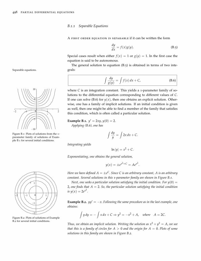
Figure B.1: Plots of solutions from the 1-parameter family of solutions of Exam-ple B.1 for several initial conditions.

Example B.1. y′ = 2xy, y(0) = 2.Applying (B.6), one has ∫ dy

y=∫

2x dx + C.

Integrating yieldsln |y| = x2 + C.

Exponentiating, one obtains the general solution,

y(x) = ±ex2+C = Aex2.

Here we have defined A = ±eC. Since C is an arbitrary constant, A is an arbitraryconstant. Several solutions in this 1-parameter family are shown in Figure B.1.

Next, one seeks a particular solution satisfying the initial condition. For y(0) =2, one finds that A = 2. So, the particular solution satisfying the initial conditionis y(x) = 2ex2

.

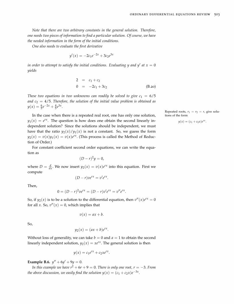
Figure B.2: Plots of solutions of ExampleB.2 for several initial conditions.

Example B.2. yy′ = −x. Following the same procedure as in the last example, oneobtains: ∫

y dy = −∫

x dx + C ⇒ y2 = −x2 + A, where A = 2C.

Thus, we obtain an implicit solution. Writing the solution as x2 + y2 = A, we seethat this is a family of circles for A > 0 and the origin for A = 0. Plots of somesolutions in this family are shown in Figure B.2.

ordinary differential equations review 499

B.1.2 Linear First Order Equations

The second type of first order equation encountered is the linearfirst order differential equation in the standard form

y′(x) + p(x)y(x) = q(x). (B.7)

In this case one seeks an integrating factor, µ(x), which is a function that onecan multiply through the equation making the left side a perfect derivative.Thus, obtaining,

ddx

[µ(x)y(x)] = µ(x)q(x). (B.8)

The integrating factor that works is µ(x) = exp(∫ x p(ξ) dξ). One can

derive µ(x) by expanding the derivative in Equation (B.8),

µ(x)y′(x) + µ′(x)y(x) = µ(x)q(x), (B.9)

and comparing this equation to the one obtained from multiplying (B.7) byµ(x) :

µ(x)y′(x) + µ(x)p(x)y(x) = µ(x)q(x). (B.10)

Note that these last two equations would be the same if the second termswere the same. Thus, we will require that

dµ(x)dx

= µ(x)p(x).

This is a separable first order equation for µ(x) whose solution is the inte-grating factor: Integrating factor.

µ(x) = exp(∫ x

p(ξ) dξ

). (B.11)

Equation (B.8) is now easily integrated to obtain the general solution tothe linear first order differential equation:

y(x) =1

µ(x)

[∫ xµ(ξ)q(ξ) dξ + C

]. (B.12)

Example B.3. xy′ + y = x, x > 0, y(1) = 0.One first notes that this is a linear first order differential equation. Solving for

y′, one can see that the equation is not separable. Furthermore, it is not in thestandard form (B.7). So, we first rewrite the equation as

dydx

+1x

y = 1. (B.13)

Noting that p(x) = 1x , we determine the integrating factor

µ(x) = exp[∫ x dξ

ξ

]= eln x = x.


Multiplying equation (B.13) by µ(x) = x, we actually get back the original equa-tion! In this case we have found that xy′ + y must have been the derivative ofsomething to start. In fact, (xy)′ = xy′ + x. Therefore, the differential equationbecomes

(xy)′ = x.

Integrating, one obtains

xy =12

x2 + C,

ory(x) =

12

x +Cx

.

Inserting the initial condition into this solution, we have 0 = 12 + C. Therefore,

C = − 12 . Thus, the solution of the initial value problem is

y(x) =12(x− 1

x).

We can verify that this is the solution. Since y′ = 12 + 1

2x2 , we have

xy′ + y =12

x +1

2x+

12

(x− 1

x

)= x.

Also, y(1) = 12 (1− 1) = 0.

Example B.4. (sin x)y′ + (cos x)y = x2.Actually, this problem is easy if you realize that the left hand side is a perfect

derivative. Namely,

ddx

((sin x)y) = (sin x)y′ + (cos x)y.

But, we will go through the process of finding the integrating factor for practice.First, we rewrite the original differential equation in standard form. We divide

the equation by sin x to obtain

y′ + (cot x)y = x2 csc x.

Then, we compute the integrating factor as

µ(x) = exp(∫ x

cot ξ dξ

)= eln(sin x) = sin x.

Using the integrating factor, the standard form equation becomes

ddx

((sin x)y) = x2.

Integrating, we have

y sin x =13

x3 + C.

So, the solution is

y(x) =(

13

x3 + C)

csc x.


B.2 Second Order Linear Differential Equations

Second order differential equations are typically harder thanfirst order. In most cases students are only exposed to second order lineardifferential equations. A general form for a second order linear differentialequation is given by

a(x)y′′(x) + b(x)y′(x) + c(x)y(x) = f (x). (B.14)

One can rewrite this equation using operator terminology. Namely, onefirst defines the differential operator L = a(x)D2 + b(x)D + c(x), whereD = d

dx . Then equation (B.14) becomes

Ly = f . (B.15)

The solutions of linear differential equations are found by making use ofthe linearity of L. Namely, we consider the vector space1 consisting of real-

1 We assume that the reader has been in-troduced to concepts in linear algebra.Later in the text we will recall the def-inition of a vector space and see that lin-ear algebra is in the background of thestudy of many concepts in the solutionof differential equations.

valued functions over some domain. Let f and g be vectors in this functionspace. L is a linear operator if for two vectors f and g and scalar a, we havethat

a. L( f + g) = L f + Lg

b. L(a f ) = aL f .

One typically solves (B.14) by finding the general solution of the homo-geneous problem,

Lyh = 0

and a particular solution of the nonhomogeneous problem,

Lyp = f .

Then, the general solution of (B.14) is simply given as y = yh + yp. This istrue because of the linearity of L. Namely,

Ly = L(yh + yp)

= Lyh + Lyp

= 0 + f = f . (B.16)

There are methods for finding a particular solution of a nonhomogeneousdifferential equation. These methods range from pure guessing, the Methodof Undetermined Coefficients, the Method of Variation of Parameters, orGreen’s functions. We will review these methods later in the chapter.

Determining solutions to the homogeneous problem, Lyh = 0, is not al-ways easy. However, many now famous mathematicians and physicists havestudied a variety of second order linear equations and they have saved usthe trouble of finding solutions to the differential equations that often ap-pear in applications. We will encounter many of these in the following


chapters. We will first begin with some simple homogeneous linear differ-ential equations.

Linearity is also useful in producing the general solution of a homoge-neous linear differential equation. If y1 and y2 are solutions of the homoge-neous equation, then the linear combination y = c1y1 + c2y2 is also a solutionof the homogeneous equation. In fact, if y1 and y2 are linearly independent,22 A set of functions {yi(x)}n

i=1 is a lin-early independent set if and only if

c1y1(x) + . . . + cnyn(x) = 0

implies ci = 0, for i = 1, . . . , n.For n = 2, c1y1(x) + c2y2(x) = 0. If

y1 and y2 are linearly dependent, thenthe coefficients are not zero andy2(x) = − c1

c2y1(x) and is a multiple of

y1(x).

then y = c1y1 + c2y2 is the general solution of the homogeneous problem.Linear independence can also be established by looking at the Wronskian

of the solutions. For a second order differential equation the Wronskian isdefined as

W(y1, y2) = y1(x)y′2(x)− y′1(x)y2(x). (B.17)

The solutions are linearly independent if the Wronskian is not zero.

B.2.1 Constant Coefficient Equations

The simplest second order differential equations are those withconstant coefficients. The general form for a homogeneous constant coeffi-cient second order linear differential equation is given as

ay′′(x) + by′(x) + cy(x) = 0, (B.18)

where a, b, and c are constants.Solutions to (B.18) are obtained by making a guess of y(x) = erx. Inserting

this guess into (B.18) leads to the characteristic equation

ar2 + br + c = 0. (B.19)

Namely, we compute the derivatives of y(x) = erx, to get y(x) = rerx, andThe characteristic equation foray′′ + by′ + cy = 0 is ar2 + br + c = 0.Solutions of this quadratic equation leadto solutions of the differential equation.

y(x) = r2erx. Inserting into (B.18), we have

0 = ay′′(x) + by′(x) + cy(x) = (ar2 + br + c)erx.

Since the exponential is never zero, we find that ar2 + br + c = 0.Two real, distinct roots, r1 and r2, givesolutions of the form

y(x) = c1er1x + c2er2x .The roots of this equation, r1, r2, in turn lead to three types of solutions

depending upon the nature of the roots. In general, we have two linearly in-dependent solutions, y1(x) = er1x and y2(x) = er2x, and the general solutionis given by a linear combination of these solutions,

y(x) = c1er1x + c2er2x.

For two real distinct roots, we are done. However, when the roots are real,but equal, or complex conjugate roots, we need to do a little more work toobtain usable solutions.

Example B.5. y′′ − y′ − 6y = 0 y(0) = 2, y′(0) = 0.The characteristic equation for this problem is r2 − r− 6 = 0. The roots of this

equation are found as r = −2, 3. Therefore, the general solution can be quicklywritten down:

y(x) = c1e−2x + c2e3x.


Note that there are two arbitrary constants in the general solution. Therefore,one needs two pieces of information to find a particular solution. Of course, we havethe needed information in the form of the initial conditions.

One also needs to evaluate the first derivative

y′(x) = −2c1e−2x + 3c2e3x

in order to attempt to satisfy the initial conditions. Evaluating y and y′ at x = 0yields

2 = c1 + c2

0 = −2c1 + 3c2 (B.20)

These two equations in two unknowns can readily be solved to give c1 = 6/5and c2 = 4/5. Therefore, the solution of the initial value problem is obtained asy(x) = 6

5 e−2x + 45 e3x.

Repeated roots, r1 = r2 = r, give solu-tions of the form

y(x) = (c1 + c2x)erx .

In the case when there is a repeated real root, one has only one solution,y1(x) = erx. The question is how does one obtain the second linearly in-dependent solution? Since the solutions should be independent, we musthave that the ratio y2(x)/y1(x) is not a constant. So, we guess the formy2(x) = v(x)y1(x) = v(x)erx. (This process is called the Method of Reduc-tion of Order.)

For constant coefficient second order equations, we can write the equa-tion as

(D− r)2y = 0,

where D = ddx . We now insert y2(x) = v(x)erx into this equation. First we

compute(D− r)verx = v′erx.

Then,0 = (D− r)2verx = (D− r)v′erx = v′′erx.

So, if y2(x) is to be a solution to the differential equation, then v′′(x)erx = 0for all x. So, v′′(x) = 0, which implies that

v(x) = ax + b.

So,y2(x) = (ax + b)erx.

Without loss of generality, we can take b = 0 and a = 1 to obtain the secondlinearly independent solution, y2(x) = xerx. The general solution is then

y(x) = c1erx + c2xerx.

Example B.6. y′′ + 6y′ + 9y = 0.In this example we have r2 + 6r + 9 = 0. There is only one root, r = −3. From

the above discussion, we easily find the solution y(x) = (c1 + c2x)e−3x.


When one has complex roots in the solution of constant coefficient equa-tions, one needs to look at the solutions

y1,2(x) = e(α±iβ)x.

We make use of Euler’s formula (See Chapter 6 for more on complex vari-ables)

eiβx = cos βx + i sin βx. (B.21)

Then, the linear combination of y1(x) and y2(x) becomes

Ae(α+iβ)x + Be(α−iβ)x = eαx[

Aeiβx + Be−iβx]

= eαx [(A + B) cos βx + i(A− B) sin βx]

≡ eαx(c1 cos βx + c2 sin βx). (B.22)

Thus, we see that we have a linear combination of two real, linearly inde-pendent solutions, eαx cos βx and eαx sin βx.Complex roots, r = α± iβ, give solutions

of the form

y(x) = eαx(c1 cos βx + c2 sin βx). Example B.7. y′′ + 4y = 0.The characteristic equation in this case is r2 + 4 = 0. The roots are pure imag-

inary roots, r = ±2i, and the general solution consists purely of sinusoidal func-tions, y(x) = c1 cos(2x) + c2 sin(2x), since α = 0 and β = 2.

Example B.8. y′′ + 2y′ + 4y = 0.The characteristic equation in this case is r2 + 2r+ 4 = 0. The roots are complex,

r = −1±√

3i and the general solution can be written as

y(x) =[c1 cos(

√3x) + c2 sin(

√3x)]

e−x.

Example B.9. y′′ + 4y = sin x.This is an example of a nonhomogeneous problem. The homogeneous problem

was actually solved in Example B.7. According to the theory, we need only seek aparticular solution to the nonhomogeneous problem and add it to the solution of thelast example to get the general solution.

The particular solution can be obtained by purely guessing, making an educatedguess, or using the Method of Variation of Parameters. We will not review all ofthese techniques at this time. Due to the simple form of the driving term, we willmake an intelligent guess of yp(x) = A sin x and determine what A needs to be.Inserting this guess into the differential equation gives (−A + 4A) sin x = sin x.So, we see that A = 1/3 works. The general solution of the nonhomogeneousproblem is therefore y(x) = c1 cos(2x) + c2 sin(2x) + 1

3 sin x.

The three cases for constant coefficient linear second order differentialequations are summarized below.


Classification of Roots of the Characteristic Equationfor Second Order Constant Coefficient ODEs

1. Real, distinct roots r1, r2. In this case the solutions corresponding toeach root are linearly independent. Therefore, the general solution issimply y(x) = c1er1x + c2er2x.

2. Real, equal roots r1 = r2 = r. In this case the solutions correspondingto each root are linearly dependent. To find a second linearly inde-pendent solution, one uses the Method of Reduction of Order. This givesthe second solution as xerx. Therefore, the general solution is found asy(x) = (c1 + c2x)erx.

3. Complex conjugate roots r1, r2 = α ± iβ. In this case the solutionscorresponding to each root are linearly independent. Making use ofEuler’s identity, eiθ = cos(θ) + i sin(θ), these complex exponentialscan be rewritten in terms of trigonometric functions. Namely, onehas that eαx cos(βx) and eαx sin(βx) are two linearly independent solu-tions. Therefore, the general solution becomes y(x) = eαx(c1 cos(βx) +c2 sin(βx)).

B.3 Forced Systems

Many problems can be modeled by nonhomogeneous second orderequations. Thus, we want to find solutions of equations of the form

Ly(x) = a(x)y′′(x) + b(x)y′(x) + c(x)y(x) = f (x). (B.23)

As noted in Section B.2, one solves this equation by finding the generalsolution of the homogeneous problem,

Lyh = 0

and a particular solution of the nonhomogeneous problem,

Lyp = f .

Then, the general solution of (B.14) is simply given as y = yh + yp.So far, we only know how to solve constant coefficient, homogeneous

equations. So, by adding a nonhomogeneous term to such equations wewill need to find the particular solution to the nonhomogeneous equation.

We could guess a solution, but that is not usually possible without a littlebit of experience. So, we need some other methods. There are two mainmethods. In the first case, the Method of Undetermined Coefficients, onemakes an intelligent guess based on the form of f (x). In the second method,one can systematically developed the particular solution. We will come backto the Method of Variation of Parameters and we will also introduce thepowerful machinery of Green’s functions later in this section.


B.3.1 Method of Undetermined Coefficients

Let’s solve a simple differential equation highlighting how we canhandle nonhomogeneous equations.

Example B.10. Consider the equation

y′′ + 2y′ − 3y = 4. (B.24)

The first step is to determine the solution of the homogeneous equation. Thus,we solve

y′′h + 2y′h − 3yh = 0. (B.25)

The characteristic equation is r2 + 2r− 3 = 0. The roots are r = 1,−3. So, we canimmediately write the solution

yh(x) = c1ex + c2e−3x.

The second step is to find a particular solution of (B.24). What possible functioncan we insert into this equation such that only a 4 remains? If we try somethingproportional to x, then we are left with a linear function after inserting x and itsderivatives. Perhaps a constant function you might think. y = 4 does not work.But, we could try an arbitrary constant, y = A.

Let’s see. Inserting y = A into (B.24), we obtain

−3A = 4.

Ah ha! We see that we can choose A = − 43 and this works. So, we have a particular

solution, yp(x) = − 43 . This step is done.

Combining the two solutions, we have the general solution to the original non-homogeneous equation (B.24). Namely,

y(x) = yh(x) + yp(x) = c1ex + c2e−3x − 43

.

Insert this solution into the equation and verify that it is indeed a solution. If wehad been given initial conditions, we could now use them to determine the arbitraryconstants.

Example B.11. What if we had a different source term? Consider the equation

y′′ + 2y′ − 3y = 4x. (B.26)

The only thing that would change is the particular solution. So, we need a guess.We know a constant function does not work by the last example. So, let’s try

yp = Ax. Inserting this function into Equation (B.26), we obtain

2A− 3Ax = 4x.

Picking A = −4/3 would get rid of the x terms, but will not cancel everything.We still have a constant left. So, we need something more general.


Let’s try a linear function, yp(x) = Ax + B. Then we get after substitution into(B.26)

2A− 3(Ax + B) = 4x.

Equating the coefficients of the different powers of x on both sides, we find a systemof equations for the undetermined coefficients:

2A− 3B = 0

−3A = 4. (B.27)

These are easily solved to obtain

A = −43

B =23

A = −89

. (B.28)

So, the particular solution is

yp(x) = −43

x− 89

.

This gives the general solution to the nonhomogeneous problem as

y(x) = yh(x) + yp(x) = c1ex + c2e−3x − 43

x− 89

.

There are general forms that you can guess based upon the form of thedriving term, f (x). Some examples are given in Table B.1. More general ap-plications are covered in a standard text on differential equations. However,the procedure is simple. Given f (x) in a particular form, you make an ap-propriate guess up to some unknown parameters, or coefficients. Insertingthe guess leads to a system of equations for the unknown coefficients. Solvethe system and you have the solution. This solution is then added to thegeneral solution of the homogeneous differential equation.

f (x) Guessanxn + an−1xn−1 + · · ·+ a1x + a0 Anxn + An−1xn−1 + · · ·+ A1x + A0

aebx Aebx

a cos ωx + b sin ωx A cos ωx + B sin ωx

Table B.1: Forms used in the Method ofUndetermined Coefficients.

Example B.12. Solvey′′ + 2y′ − 3y = 2e−3x. (B.29)

According to the above, we would guess a solution of the form yp = Ae−3x.Inserting our guess, we find

0 = 2e−3x.

Oops! The coefficient, A, disappeared! We cannot solve for it. What went wrong?The answer lies in the general solution of the homogeneous problem. Note that ex

and e−3x are solutions to the homogeneous problem. So, a multiple of e−3x will notget us anywhere. It turns out that there is one further modification of the method.


If the driving term contains terms that are solutions of the homogeneous problem,then we need to make a guess consisting of the smallest possible power of x timesthe function which is no longer a solution of the homogeneous problem. Namely,we guess yp(x) = Axe−3x and differentiate this guess to obtain the derivativesy′p = A(1− 3x)e−3x and y′′p = A(9x− 6)e−3x.

Inserting these derivatives into the differential equation, we obtain

[(9x− 6) + 2(1− 3x)− 3x]Ae−3x = 2e−3x.

Comparing coefficients, we have

−4A = 2.

So, A = −1/2 and yp(x) = − 12 xe−3x. Thus, the solution to the problem is

y(x) =(

2− 12

x)

e−3x.

Modified Method of Undetermined Coefficients

In general, if any term in the guess yp(x) is a solution of the homogeneousequation, then multiply the guess by xk, where k is the smallest positiveinteger such that no term in xkyp(x) is a solution of the homogeneousproblem.

B.3.2 Periodically Forced Oscillations

A special type of forcing is periodic forcing. Realistic oscillations willdampen and eventually stop if left unattended. For example, mechanicalclocks are driven by compound or torsional pendula and electric oscilla-tors are often designed with the need to continue for long periods of time.However, they are not perpetual motion machines and will need a peri-odic injection of energy. This can be done systematically by adding periodicforcing. Another simple example is the motion of a child on a swing in thepark. This simple damped pendulum system will naturally slow down toequilibrium (stopped) if left alone. However, if the child pumps energy intothe swing at the right time, or if an adult pushes the child at the right time,then the amplitude of the swing can be increased.

There are other systems, such as airplane wings and long bridge spans,in which external driving forces might cause damage to the system. A wellknow example is the wind induced collapse of the Tacoma Narrows Bridgedue to strong winds. Of course, if one is not careful, the child in theThe Tacoma Narrows Bridge opened in

Washington State (U.S.) in mid 1940.However, in November of the same yearthe winds excited a transverse mode ofvibration, which eventually (in a fewhours) lead to large amplitude oscilla-tions and then collapse.

last example might get too much energy pumped into the system causing asimilar failure of the desired motion.

While there are many types of forced systems, and some fairly compli-cated, we can easily get to the basic characteristics of forced oscillations bymodifying the mass-spring system by adding an external, time-dependent,driving force. Such as system satisfies the equation

mx + b(x) + kx = F(t), (B.30)


where m is the mass, b is the damping constant, k is the spring constant,and F(t) is the driving force. If F(t) is of simple form, then we can employthe Method of Undetermined Coefficients. Since the systems we have con-sidered so far are similar, one could easily apply the following to pendulaor circuits.

k m

b

F cos w t0

Figure B.3: An external driving force isadded to the spring-mass-damper sys-tem.

As the damping term only complicates the solution, we will consider thesimpler case of undamped motion and assume that b = 0. Furthermore,we will introduce a sinusoidal driving force, F(t) = F0 cos ωt in order tostudy periodic forcing. This leads to the simple periodically driven mass ona spring system

mx + kx = F0 cos ωt. (B.31)

In order to find the general solution, we first obtain the solution to thehomogeneous problem,

xh = c1 cos ω0t + c2 sin ω0t,

where ω0 =√

km . Next, we seek a particular solution to the nonhomoge-

neous problem. We will apply the Method of Undetermined Coefficients.A natural guess for the particular solution would be to use xp = A cos ωt+

B sinωt. However, recall that the guess should not be a solution of the ho-mogeneous problem. Comparing xp with xh, this would hold if ω 6= ω0.Otherwise, one would need to use the Modified Method of UndeterminedCoefficients as described in the last section. So, we have two cases to con-sider. Dividing through by the mass, we solve

the simple driven system,

x + ω20 x =

F0

mcos ωt.

Example B.13. Solve x + ω20x = F0

m cos ωt, for ω 6= ω0.In this case we continue with the guess xp = A cos ωt + B sinωt. Since there

is no damping term, one quickly finds that B = 0. Inserting xp = A cos ωt intothe differential equation, we find that(

−ω2 + ω20

)A cos ωt =

F0

mcos ωt.

Solving for A, we obtain

A =F0

m(ω20 −ω2)

.

The general solution for this case is thus,

x(t) = c1 cos ω0t + c2 sin ω0t +F0

m(ω20 −ω2)

cos ωt. (B.32)

Example B.14. Solve x + ω20x = F0

m cos ω0t.In this case, we need to employ the Modified Method of Undetermined Coef-

ficients. So, we make the guess xp = t (A cos ω0t + B sinω0t) . Since there isno damping term, one finds that A = 0. Inserting the guess in to the differentialequation, we find that

B =F0

2mω0,

or the general solution is

x(t) = c1 cos ω0t + c2 sin ω0t +F0

2mωt sin ωt. (B.33)


The general solution to the problem is thus

x(t) = c1 cos ω0t + c2 sin ω0t +

{ F0m(ω2

0−ω2)cos ωt, ω 6= ω0,

F02mω0

t sin ω0t, ω = ω0.(B.34)

Special cases of these solutions provide interesting physics, which canbe explored by the reader in the homework. In the case that ω = ω0, wesee that the solution tends to grow as t gets large. This is what is called aresonance. Essentially, one is driving the system at its natural frequency. Asthe system is moving to the left, one pushes it to the left. If it is moving tothe right, one is adding energy in that direction. This forces the amplitudeof oscillation to continue to grow until the system breaks. An example ofsuch an oscillation is shown in Figure B.4.

Figure B.4: Plot of

x(t) = 5 cos 2t +12

t sin 2t,

a solution of x + 4x = 2 cos 2t showingresonance.

In the case that ω 6= ω0, one can rewrite the solution in a simple form.Let’s choose the initial conditions that c1 = −F0/(m(ω2

0−ω2)), c2 = 0. Thenone has (see Problem ??)

x(t) =2F0

m(ω20 −ω2)

sin(ω0 −ω)t

2sin

(ω0 + ω)t2

. (B.35)

For values of ω near ω0, one finds the solution consists of a rapid os-cillation, due to the sin (ω0+ω)t

2 factor, with a slowly varying amplitude,2F0

m(ω20−ω2)

sin (ω0−ω)t2 . The reader can investigate this solution.

Figure B.5: Plot of

x(t) =1

249

(2045 cos 2t− 800 cos

4320

t)

,

a solution of x + 4x = 2 cos 2.15t.

This slow variation is called a beat and the beat frequency is given by f =|ω0−ω|

4π . In Figure B.5 we see the high frequency oscillations are containedby the lower beat frequency, f = 0.15

4π s. This corresponds to a period ofT = 1/ f ≈ 83.7 Hz, which looks about right from the figure.

Example B.15. Solve x + x = 2 cos ωt, x(0) = 0, x(0) = 0, for ω = 1, 1.15. Foreach case, we need the solution of the homogeneous problem,

xh(t) = c1 cos t + c2 sin t.

The particular solution depends on the value of ω.For ω = 1, the driving term, 2 cos ωt, is a solution of the homogeneous problem.

Thus, we assumexp(t) = At cos t + Bt sin t.

Inserting this into the differential equation, we find A = 0 and B = 1. So, thegeneral solution is

x(t) = c1 cos t + c2 sin t + t sin t.

Imposing the initial conditions, we find

x(t) = t sin t.

This solution is shown in Figure B.6.

Figure B.6: Plot of

x(t) = t sin 2t,

a solution of x + x = 2 cos t.

For ω = 1.15, the driving term, 2 cos ω1.15t, is not a solution of the homoge-neous problem. Thus, we assume

xp(t) = A cos 1.15t + B sin 1.15t.


Inserting this into the differential equation, we find A = − 800129 and B = 0. So, the

general solution is

x(t) = c1 cos t + c2 sin t− 800129

cos t.

Imposing the initial conditions, we find

x(t) =800129

(cos t− cos 1.15t) .

This solution is shown in Figure B.7. The beat frequency in this case is the same aswith Figure B.5.

Figure B.7: Plot of

x(t) =800129

(cos t− cos

2320

t)

,

a solution of x + x = 2 cos 1.15t.

B.3.3 Method of Variation of Parameters

A more systematic way to find particular solutions is through the useof the Method of Variation of Parameters. The derivation is a little detailedand the solution is sometimes messy, but the application of the method isstraight forward if you can do the required integrals. We will first derivethe needed equations and then do some examples.

We begin with the nonhomogeneous equation. Let’s assume it is of thestandard form

a(x)y′′(x) + b(x)y′(x) + c(x)y(x) = f (x). (B.36)

We know that the solution of the homogeneous equation can be written interms of two linearly independent solutions, which we will call y1(x) andy2(x) :

yh(x) = c1y1(x) + c2y2(x).

Replacing the constants with functions, then we no longer have a solutionto the homogeneous equation. Is it possible that we could stumble acrossthe right functions with which to replace the constants and somehow endup with f (x) when inserted into the left side of the differential equation? Itturns out that we can.

So, let’s assume that the constants are replaced with two unknown func-tions, which we will call c1(x) and c2(x). This change of the parametersis where the name of the method derives. Thus, we are assuming that aparticular solution takes the form We assume the nonhomogeneous equa-

tion has a particular solution of the form

yp(x) = c1(x)y1(x) + c2(x)y2(x).yp(x) = c1(x)y1(x) + c2(x)y2(x). (B.37)

If this is to be a solution, then insertion into the differential equation shouldmake the equation hold. To do this we will first need to compute somederivatives.

The first derivative is given by

y′p(x) = c1(x)y′1(x) + c2(x)y′2(x) + c′1(x)y1(x) + c′2(x)y2(x). (B.38)


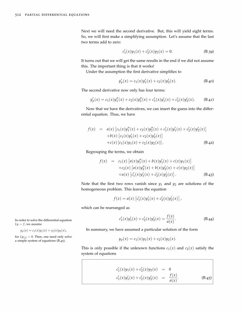
Next we will need the second derivative. But, this will yield eight terms.So, we will first make a simplifying assumption. Let’s assume that the lasttwo terms add to zero:

c′1(x)y1(x) + c′2(x)y2(x) = 0. (B.39)

It turns out that we will get the same results in the end if we did not assumethis. The important thing is that it works!

Under the assumption the first derivative simplifies to

y′p(x) = c1(x)y′1(x) + c2(x)y′2(x). (B.40)

The second derivative now only has four terms:

y′p(x) = c1(x)y′′1 (x) + c2(x)y′′2 (x) + c′1(x)y′1(x) + c′2(x)y′2(x). (B.41)

Now that we have the derivatives, we can insert the guess into the differ-ential equation. Thus, we have

f (x) = a(x)[c1(x)y′′1 (x) + c2(x)y′′2 (x) + c′1(x)y′1(x) + c′2(x)y′2(x)

]+b(x)

[c1(x)y′1(x) + c2(x)y′2(x)

]+c(x) [c1(x)y1(x) + c2(x)y2(x)] . (B.42)

Regrouping the terms, we obtain

f (x) = c1(x)[a(x)y′′1 (x) + b(x)y′1(x) + c(x)y1(x)

]+c2(x)

[a(x)y′′2 (x) + b(x)y′2(x) + c(x)y2(x)

]+a(x)

[c′1(x)y′1(x) + c′2(x)y′2(x)

]. (B.43)

Note that the first two rows vanish since y1 and y2 are solutions of thehomogeneous problem. This leaves the equation

f (x) = a(x)[c′1(x)y′1(x) + c′2(x)y′2(x)

],

which can be rearranged as

c′1(x)y′1(x) + c′2(x)y′2(x) =f (x)a(x)

. (B.44)

In summary, we have assumed a particular solution of the form

yp(x) = c1(x)y1(x) + c2(x)y2(x).

This is only possible if the unknown functions c1(x) and c2(x) satisfy thesystem of equations

In order to solve the differential equationLy = f , we assume

yp(x) = c1(x)y1(x) + c2(x)y2(x),

for Ly1,2 = 0. Then, one need only solvea simple system of equations (B.45).

c′1(x)y1(x) + c′2(x)y2(x) = 0

c′1(x)y′1(x) + c′2(x)y′2(x) =f (x)a(x)

. (B.45)


System (B.45) can be solved as

c′1(x) = − f y2

aW(y1, y2),

c′1(x) =f y1

aW(y1, y2),

where W(y1, y2) = y1y′2 − y′1y2 is theWronskian. We use this solution in thenext section.

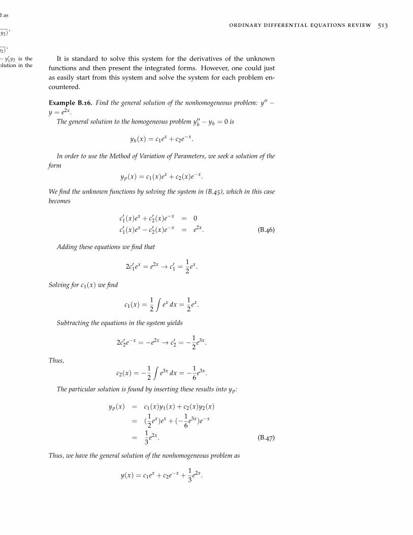
It is standard to solve this system for the derivatives of the unknownfunctions and then present the integrated forms. However, one could justas easily start from this system and solve the system for each problem en-countered.

Example B.16. Find the general solution of the nonhomogeneous problem: y′′ −y = e2x.

The general solution to the homogeneous problem y′′h − yh = 0 is

yh(x) = c1ex + c2e−x.

In order to use the Method of Variation of Parameters, we seek a solution of theform

yp(x) = c1(x)ex + c2(x)e−x.

We find the unknown functions by solving the system in (B.45), which in this casebecomes

c′1(x)ex + c′2(x)e−x = 0

c′1(x)ex − c′2(x)e−x = e2x. (B.46)

Adding these equations we find that

2c′1ex = e2x → c′1 =12

ex.

Solving for c1(x) we find

c1(x) =12

∫ex dx =

12

ex.

Subtracting the equations in the system yields

2c′2e−x = −e2x → c′2 = −12

e3x.

Thus,

c2(x) = −12

∫e3x dx = −1

6e3x.

The particular solution is found by inserting these results into yp:

yp(x) = c1(x)y1(x) + c2(x)y2(x)

= (12

ex)ex + (−16

e3x)e−x

=13

e2x. (B.47)

Thus, we have the general solution of the nonhomogeneous problem as

y(x) = c1ex + c2e−x +13

e2x.


Example B.17. Now consider the problem: y′′ + 4y = sin x.The solution to the homogeneous problem is

yh(x) = c1 cos 2x + c2 sin 2x. (B.48)

We now seek a particular solution of the form

yh(x) = c1(x) cos 2x + c2(x) sin 2x.

We let y1(x) = cos 2x and y2(x) = sin 2x, a(x) = 1, f (x) = sin x in system(B.45):

c′1(x) cos 2x + c′2(x) sin 2x = 0

−2c′1(x) sin 2x + 2c′2(x) cos 2x = sin x. (B.49)

Now, use your favorite method for solving a system of two equations and twounknowns. In this case, we can multiply the first equation by 2 sin 2x and thesecond equation by cos 2x. Adding the resulting equations will eliminate the c′1terms. Thus, we have

c′2(x) =12

sin x cos 2x =12(2 cos2 x− 1) sin x.

Inserting this into the first equation of the system, we have

c′1(x) = −c′2(x)sin 2xcos 2x

= −12

sin x sin 2x = − sin2 x cos x.

These can easily be solved:

c2(x) =12

∫(2 cos2 x− 1) sin x dx =

12(cos x− 2

3cos3 x).

c1(x) = −∫

sinx cos x dx = −13

sin3 x.

The final step in getting the particular solution is to insert these functions intoyp(x). This gives

yp(x) = c1(x)y1(x) + c2(x)y2(x)

= (−13

sin3 x) cos 2x + (12

cos x− 13

cos3 x) sin x

=13

sin x. (B.50)

So, the general solution is

y(x) = c1 cos 2x + c2 sin 2x +13

sin x. (B.51)

B.4 Cauchy-Euler Equations

Another class of solvable linear differential equations that isof interest are the Cauchy-Euler type of equations, also referred to in somebooks as Euler’s equation. These are given by

ax2y′′(x) + bxy′(x) + cy(x) = 0. (B.52)


Note that in such equations the power of x in each of the coefficients matchesthe order of the derivative in that term. These equations are solved in amanner similar to the constant coefficient equations.

One begins by making the guess y(x) = xr. Inserting this function andits derivatives,

y′(x) = rxr−1, y′′(x) = r(r− 1)xr−2,

into Equation (B.52), we have

[ar(r− 1) + br + c] xr = 0.

Since this has to be true for all x in the problem domain, we obtain thecharacteristic equation The solutions of Cauchy-Euler equations

can be found using the characteristicequation ar(r− 1) + br + c = 0.ar(r− 1) + br + c = 0. (B.53)

Just like the constant coefficient differential equation, we have a quadraticequation and the nature of the roots again leads to three classes of solutions.If there are two real, distinct roots, then the general solution takes the formy(x) = c1xr1 + c2xr2 . For two real, distinct roots, the general

solution takes the form

y(x) = c1xr1 + c2xr2 .Example B.18. Find the general solution: x2y′′ + 5xy′ + 12y = 0.

As with the constant coefficient equations, we begin by writing down the char-acteristic equation. Doing a simple computation,

0 = r(r− 1) + 5r + 12

= r2 + 4r + 12

= (r + 2)2 + 8,

−8 = (r + 2)2, (B.54)

one determines the roots are r = −2 ± 2√

2i. Therefore, the general solution isy(x) =

[c1 cos(2

√2 ln |x|) + c2 sin(2

√2 ln |x|)

]x−2

Deriving the solution for Case 2 for the Cauchy-Euler equations works inthe same way as the second for constant coefficient equations, but it is a bitmessier. First note that for the real root, r = r1, the characteristic equationhas to factor as (r− r1)

2 = 0. Expanding, we have

r2 − 2r1r + r21 = 0.

The general characteristic equation is

ar(r− 1) + br + c = 0.

Dividing this equation by a and rewriting, we have

r2 + (ba− 1)r +

ca= 0.

Comparing equations, we find

ba= 1− 2r1,

ca= r2

1.


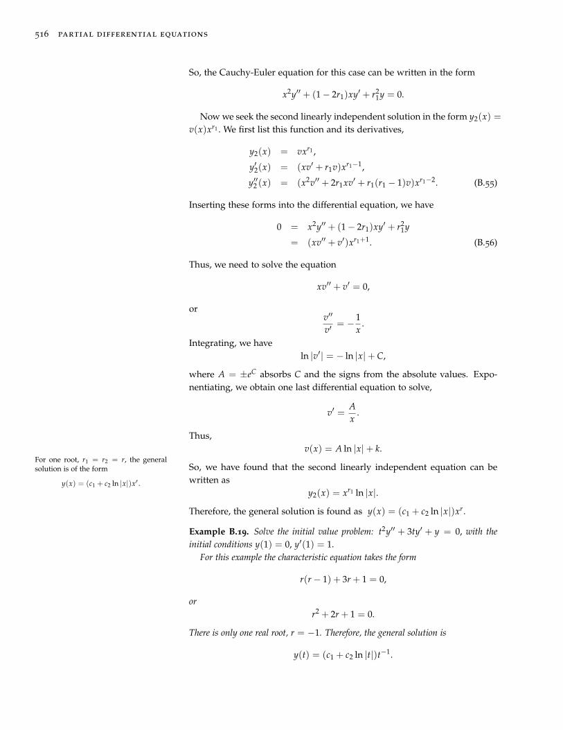
So, the Cauchy-Euler equation for this case can be written in the form

x2y′′ + (1− 2r1)xy′ + r21y = 0.

Now we seek the second linearly independent solution in the form y2(x) =v(x)xr1 . We first list this function and its derivatives,

y2(x) = vxr1 ,

y′2(x) = (xv′ + r1v)xr1−1,

y′′2 (x) = (x2v′′ + 2r1xv′ + r1(r1 − 1)v)xr1−2. (B.55)

Inserting these forms into the differential equation, we have

0 = x2y′′ + (1− 2r1)xy′ + r21y

= (xv′′ + v′)xr1+1. (B.56)

Thus, we need to solve the equation

xv′′ + v′ = 0,

orv′′

v′= − 1

x.

Integrating, we haveln |v′| = − ln |x|+ C,

where A = ±eC absorbs C and the signs from the absolute values. Expo-nentiating, we obtain one last differential equation to solve,

v′ =Ax

.

Thus,v(x) = A ln |x|+ k.

So, we have found that the second linearly independent equation can bewritten as

y2(x) = xr1 ln |x|.

Therefore, the general solution is found as y(x) = (c1 + c2 ln |x|)xr.

For one root, r1 = r2 = r, the generalsolution is of the form

y(x) = (c1 + c2 ln |x|)xr .

Example B.19. Solve the initial value problem: t2y′′ + 3ty′ + y = 0, with theinitial conditions y(1) = 0, y′(1) = 1.

For this example the characteristic equation takes the form

r(r− 1) + 3r + 1 = 0,

orr2 + 2r + 1 = 0.

There is only one real root, r = −1. Therefore, the general solution is

y(t) = (c1 + c2 ln |t|)t−1.


However, this problem is an initial value problem. At t = 1 we know the valuesof y and y′. Using the general solution, we first have that

0 = y(1) = c1.

Thus, we have so far that y(t) = c2 ln |t|t−1. Now, using the second condition and

y′(t) = c2(1− ln |t|)t−2,

we have

1 = y(1) = c2.

Therefore, the solution of the initial value problem is y(t) = ln |t|t−1.For complex conjugate roots, r = α± iβ,the general solution takes the form

y(x) = xα(c1 cos(β ln |x|)+ c2 sin(β ln |x|)).

We now turn to the case of complex conjugate roots, r = α± iβ. Whendealing with the Cauchy-Euler equations, we have solutions of the formy(x) = xα+iβ. The key to obtaining real solutions is to first rewrite xy :

xy = eln xy= ey ln x.

Thus, a power can be written as an exponential and the solution can bewritten as

y(x) = xα+iβ = xαeiβ ln x, x > 0.

Recalling that

eiβ ln x = cos(β ln |x|) + i sin(β ln |x|),

we can now find two real, linearly independent solutions, xα cos(β ln |x|)and xα sin(β ln |x|) following the same steps as earlier for the constant coef-ficient case. This gives the general solution as

y(x) = xα(c1 cos(β ln |x|) + c2 sin(β ln |x|)).

Example B.20. Solve: x2y′′ − xy′ + 5y = 0.The characteristic equation takes the form

r(r− 1)− r + 5 = 0,

or

r2 − 2r + 5 = 0.

The roots of this equation are complex, r1,2 = 1± 2i. Therefore, the general solutionis y(x) = x(c1 cos(2 ln |x|) + c2 sin(2 ln |x|)).

The three cases are summarized in the table below.


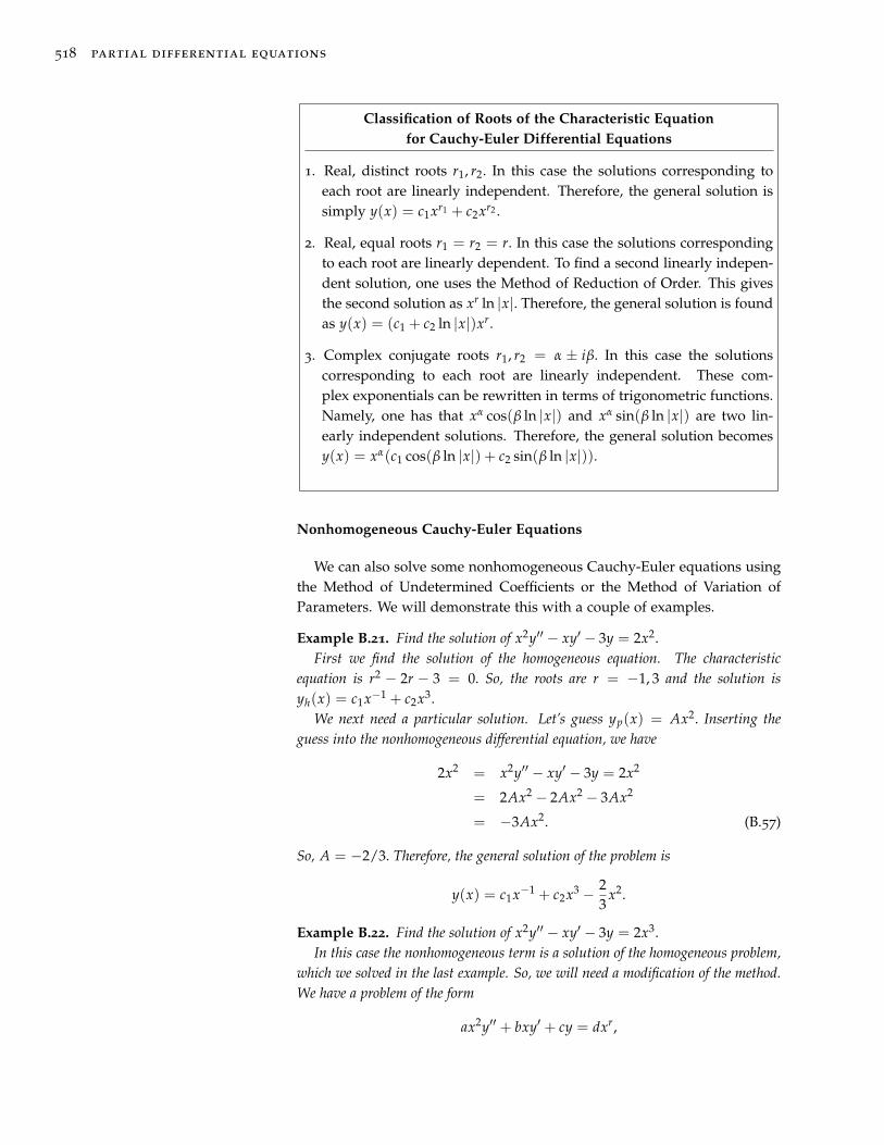
Classification of Roots of the Characteristic Equationfor Cauchy-Euler Differential Equations

1. Real, distinct roots r1, r2. In this case the solutions corresponding toeach root are linearly independent. Therefore, the general solution issimply y(x) = c1xr1 + c2xr2 .

2. Real, equal roots r1 = r2 = r. In this case the solutions correspondingto each root are linearly dependent. To find a second linearly indepen-dent solution, one uses the Method of Reduction of Order. This givesthe second solution as xr ln |x|. Therefore, the general solution is foundas y(x) = (c1 + c2 ln |x|)xr.

3. Complex conjugate roots r1, r2 = α ± iβ. In this case the solutionscorresponding to each root are linearly independent. These com-plex exponentials can be rewritten in terms of trigonometric functions.Namely, one has that xα cos(β ln |x|) and xα sin(β ln |x|) are two lin-early independent solutions. Therefore, the general solution becomesy(x) = xα(c1 cos(β ln |x|) + c2 sin(β ln |x|)).

Nonhomogeneous Cauchy-Euler Equations

We can also solve some nonhomogeneous Cauchy-Euler equations usingthe Method of Undetermined Coefficients or the Method of Variation ofParameters. We will demonstrate this with a couple of examples.

Example B.21. Find the solution of x2y′′ − xy′ − 3y = 2x2.First we find the solution of the homogeneous equation. The characteristic

equation is r2 − 2r − 3 = 0. So, the roots are r = −1, 3 and the solution isyh(x) = c1x−1 + c2x3.

We next need a particular solution. Let’s guess yp(x) = Ax2. Inserting theguess into the nonhomogeneous differential equation, we have

2x2 = x2y′′ − xy′ − 3y = 2x2

= 2Ax2 − 2Ax2 − 3Ax2

= −3Ax2. (B.57)

So, A = −2/3. Therefore, the general solution of the problem is

y(x) = c1x−1 + c2x3 − 23

x2.

Example B.22. Find the solution of x2y′′ − xy′ − 3y = 2x3.In this case the nonhomogeneous term is a solution of the homogeneous problem,

which we solved in the last example. So, we will need a modification of the method.We have a problem of the form

ax2y′′ + bxy′ + cy = dxr,


where r is a solution of ar(r− 1) + br + c = 0. Let’s guess a solution of the formy = Axr ln x. Then one finds that the differential equation reduces to Axr(2ar −a + b) = dxr. [You should verify this for yourself.]

With this in mind, we can now solve the problem at hand. Let yp = Ax3 ln x.Inserting into the equation, we obtain 4Ax3 = 2x3, or A = 1/2. The generalsolution of the problem can now be written as

y(x) = c1x−1 + c2x3 +12

x3 ln x.

Example B.23. Find the solution of x2y′′ − xy′ − 3y = 2x3 using Variation ofParameters.

As noted in the previous examples, the solution of the homogeneous problem hastwo linearly independent solutions, y1(x) = x−1 and y2(x) = x3. Assuming aparticular solution of the form yp(x) = c1(x)y1(x) + c2(x)y2(x), we need to solvethe system (B.45):

c′1(x)x−1 + c′2(x)x3 = 0

−c′1(x)x−2 + 3c′2(x)x2 =2x3

x2 = 2x. (B.58)

From the first equation of the system we have c′1(x) = −x4c′2(x). Substitutingthis into the second equation gives c′2(x) = 1

2x . So, c2(x) = 12 ln |x| and, therefore,

c1(x) = 18 x4. The particular solution is

yp(x) = c1(x)y1(x) + c2(x)y2(x) =18

x3 +12

x3 ln |x|.

Adding this to the homogeneous solution, we obtain the same solution as in the lastexample using the Method of Undetermined Coefficients. However, since 1

8 x3 is asolution of the homogeneous problem, it can be absorbed into the first terms, leaving

y(x) = c1x−1 + c2x3 +12

x3 ln x.

Problems

1. Find all of the solutions of the first order differential equations. Whenan initial condition is given, find the particular solution satisfying that con-dition.

a.dydx

=ex

2y.

b.dydt

= y2(1 + t2), y(0) = 1.

c.dydx

=

√1− y2

x.

d. xy′ = y(1− 2y), y(1) = 2.

e. y′ − (sin x)y = sin x.

f. xy′ − 2y = x2, y(1) = 1.


g.dsdt

+ 2s = st2, , s(0) = 1.

h. x′ − 2x = te2t.

i.dydx

+ y = sin x, y(0) = 0.

j.dydx− 3

xy = x3, y(1) = 4.

2. Consider the differential equation

dydx

=xy− x

1 + y.

a. Find the 1-parameter family of solutions (general solution) of thisequation.

b. Find the solution of this equation satisfying the initial conditiony(0) = 1. Is this a member of the 1-parameter family?

3. Identify the type of differential equation. Find the general solution andplot several particular solutions. Also, find the singular solution if one ex-ists.

a. y = xy′ + 1y′ .

b. y = 2xy′ + ln y′.

c. y′ + 2xy = 2xy2.

d. y′ + 2xy = y2ex2.

4. Find all of the solutions of the second order differential equations. Whenan initial condition is given, find the particular solution satisfying that con-dition.

a. y′′ − 9y′ + 20y = 0.

b. y′′ − 3y′ + 4y = 0, y(0) = 0, y′(0) = 1.

c. 8y′′ + 4y′ + y = 0, y(0) = 1, y′(0) = 0.

d. x′′ − x′ − 6x = 0 for x = x(t).

5. Verify that the given function is a solution and use Reduction of Orderto find a second linearly independent solution.

a. x2y′′ − 2xy′ − 4y = 0, y1(x) = x4.

b. xy′′ − y′ + 4x3y = 0, y1(x) = sin(x2).

6. Prove that y1(x) = sinh x and y2(x) = 3 sinh x − 2 cosh x are linearlyindependent solutions of y′′ − y = 0. Write y3(x) = cosh x as a linear com-bination of y1 and y2.

7. Consider the nonhomogeneous differential equation x′′− 3x′+ 2x = 6e3t.

a. Find the general solution of the homogenous equation.

b. Find a particular solution using the Method of Undetermined Co-efficients by guessing xp(t) = Ae3t.


c. Use your answers in the previous parts to write down the generalsolution for this problem.

8. Find the general solution of the given equation by the method given.

a. y′′ − 3y′ + 2y = 10. Method of Undetermined Coefficients.

b. y′′ + y′ = 3x2. Variation of Parameters.

9. Use the Method of Variation of Parameters to determine the generalsolution for the following problems.

a. y′′ + y = tan x.

b. y′′ − 4y′ + 4y = 6xe2x.

10. Instead of assuming that c′1y1 + c′2y2 = 0 in the derivation of the solu-tion using Variation of Parameters, assume that c′1y1 + c′2y2 = h(x) for anarbitrary function h(x) and show that one gets the same particular solution.

11. Find all of the solutions of the second order differential equations forx > 0.. When an initial condition is given, find the particular solutionsatisfying that condition.

a. x2y′′ + 3xy′ + 2y = 0.

b. x2y′′ − 3xy′ + 3y = 0.

c. x2y′′ + 5xy′ + 4y = 0.

d. x2y′′ − 2xy′ + 3y = 0.

e. x2y′′ + 3xy′ − 3y = x2.

b ordinary differential equations reviewpeople.uncw.edu/hermanr/pde1/pdebook/oderev.pdf · b...

Documents