Lloyd Chua

S1148054

AY 2013/2014 BEng Mechanical Engineering Individual Project

Final Report

Abstract

Cells are the most fundamental biological units of living organisms and their rheological and mechanical properties are responsible for various biological processes such as differentiation, growth, and cancer metastasis. A finite element model was designed and implemented to simulate Atomic Force Microscopy (AFM) experiments for the study of the sub-cellular mechanical properties that contribute towards the measured elasticity of a cell adherent on a substrate. Between cell aspect ratios (height/length) of 1/5 to 1/20, parametric variations of individual sub-cellular properties yielded elasticity values ranging up to 260%, 175%, and 129% for the cytoplasm, plasma membrane, and nucleus, respectively. However, the results of the parametric study indicated that the aspect ratio of a cell had the most significant influence on the measurement of cell elasticity using AFM, which accounted for variations in Young’s modulus of up to 331%. The cell shape was found to be the predominant influence as it governs the arrangement of sub-cellular components being deformed by an AFM indenter for the measurement of cell elasticity.

LLOYD CHUA | S1148054 | AY 2013/14 2

Personal Statement The project’s primary objective of conceptualising, designing and implementing a finite element model of a living cell was previously attempted by a BEng student in the academic year of 2012/13. However, only a finite element model of a tensegrity structure (for which an analytical solution exists) transpired from the previous project. Furthermore, as the virtual files from the previous project were irretrievable for further development, no intellectual material from previous project was used and instead, a different modelling approach was proposed for this project.

Meetings with the project supervisor (Dr. Andy Downes) were held on a weekly basis. The consultations reaped a variety of ideas that were implemented within the project and established the fundamental requirements of which the cell model was to perform. The cell model was to simulate the major sub-cellular components with mechanical properties that can be parametrically varied for the purpose of investigating the individual mechanical contributions of each sub-cellular component on the local Young’s modulus of the cell. The cell model was initially intended to simulate experimental AFM measurements of primary and secondary cancer cells (A. Downes, unpublished). However, this was not possible as the AFM measurements were unavailable within the timeline of the project. Therefore, the cell model was validated against other existing AFM experiments, and a parametric study of the primary and secondary cancer cells was omitted.

A tensegrity-continuum finite element model was determined to be the most suitable approach after the conduct of a literature review as it was assessed to be able to provide acceptably accurate results as well as being achievable within the project timeline. The preliminary results of the model were also deliberated against experimental cell behaviours with the project supervisor, which aided in the refinement of the cell model. The findings presented in this report, such as the design and implementation of the model and the graphical user interface (GUI), as well as the analysis of the simulations were completed by the individual student. Experimental measurements from published literature were referenced in the validation of the model.

With any attempt to model the physics of reality, there was a substantial degree of uncertainty as to whether a model that could replicate the real-world results could be developed within the limited timeline. While most of the work presented in the report consists of results and analysis of the simulations, the majority of the project’s efforts were spent on the development of the model itself. Even with the conceptualisation of the model finalised, an abundance of difficulties manifested at every stage of the model’s development. These difficulties can be visualised in the steep learning curve of finite element software, in which a model can be successfully simulated only when all required simulation conditions are clearly defined. Coupled with the complexity of multi-component contact problems and ambiguous error reports, a significant portion of trial-and-error was involved in the project’s efforts.

_____________________ _____________________ Student’s Signature Date of Signature

LLOYD CHUA | S1148054 | AY 2013/14 3

Table of Contents 1 INTRODUCTION 4

1.1 PROJECT OBJECTIVES 4 1.2 PROJECT PLANNING AND MANAGEMENT 5

2 LITERATURE REVIEW 6

2.1 CELL BIOLOGY 6 2.1.1 PLASMA MEMBRANE 6 2.1.2 NUCLEUS 6 2.1.3 CYTOSKELETON 7 2.1.4 CYTOPLASM 8 2.1.5 EXTRACELLULAR MATRIX 8 2.2 OVERVIEW OF MECHANICAL MODELS 9 2.2.1 CORTICAL SHELL-LIQUID CORE MODELS 9 2.2.2 POWER-LAW DAMPING MODEL 11 2.2.3 SOLID MODELS 11 2.2.4 OPEN-CELL FOAM MODEL 12 2.2.5 PRE-STRESSED CABLE NETWORK MODEL 12 2.2.6 TENSEGRITY MODEL 14 2.2.7 FINITE CONTINUUM-TENSEGRITY INTEGRATION WITHIN A FINITE ELEMENT MODEL 16 2.2.8 CONTINUUM-MICROSTRUCTURAL NETWORK WITHIN A FINITE ELEMENT MODEL 16 2.2.9 SUMMARY OF LITERATURE REVIEW 17

3 MODELLING METHODOLOGY 18

3.1 MODEL GENERATION 18 3.2 PRE-STRESSING 20 3.3 LOADING CONDITIONS 21

4 SIMULATION RESULTS AND ANALYSIS 24

4.1 MODEL VALIDATION: COMPARISON WITH EXPERIMENTAL MEASUREMENTS 24 4.1.1 MODELLING AN ENDOTHELIAL CELL 24 4.1.2 COMPARISON OF SIMULATED FORCE-DISTANCE W/ EXPERIMENTAL MEASUREMENTS 26 4.1.3 COMPARISON OF SIMULATED YOUNG’S MODULUS W/ EXPERIMENTAL MEASUREMENTS 27 4.1.4 DETERMINING THE IDEAL INDENTER SHAPE FOR THE PARAMETRIC SIMULATIONS 29 4.2 PARAMETRIC VARIATION OF VARIABLES 30 4.2.1 INFLUENCE OF INDENTATION LOCATION ON YOUNG’S MODULUS 30 4.2.2 INFLUENCE OF CELL ASPECT RATIO ON YOUNG’S MODULUS 32 4.2.3 VARYING MEMBRANE, CYTOPLASM AND NUCLEUS YOUNG’S MODULUS 33 4.2.4 VARYING CYTOPLASM POISSON’S RATIO 35 4.2.5 SIMULATING PRIMARY AND SECONDARY CANCER CELLS 37 4.2.6 LIMITATIONS 40

5 CONCLUSIONS 41

REFERENCES 41

APPENDIX A: MODEL GENERATING GUI DOCUMENTATION 47

LLOYD CHUA | S1148054 | AY 2013/14 4

1 Introduction Various biological processes such as differentiation, growth, and cancer metastasis (development and spread of secondary malignant cancerous cells) are influenced by the mechanical properties of a cell and its extra-cellular matrix [1–4]. For example, cancer cells with increased compliance or deformability were found to multiply and spread at higher rates as compared to the surrounding healthy cells, thereby linking the mechanical properties of cancer cells as one of the main contributing factors to the division and migration that drives cancer progression [5]. A decrease in a cell’s stiffness was also found to increase its potential for malignancy and metastasis [6,7].

A mechanical model of a cell that can be varied in size and shape, which is able to mimic the mechanical behaviour of living cells, can provide some understanding of the factors that govern the mechanics of cells. A convincing mechanical model may also aid in the understanding of the factors that contribute towards cancer metastasis and how to control or minimise it.

Furthermore, the measurement of cell elasticity provides a method that can be used to distinguish between different types of cells such as healthy cells, primary and secondary cancer cells [7–9]. However, experimental measurements of cell elasticity using Atomic Force Microscopy (AFM) have yielded variations of values within individual cells adherent on a substrate, as well as between cells located at the centre and the edges of a cell colony (A. Downes, unpublished).

Therefore, the verification of experimental measurements with a mechanical model in which the cell parameters and boundary conditions such as, the aspect ratio of the cell spread, the relative size of nucleus, the properties and density of cytoskeletal filaments, and the environmental factors (i.e. cells existing within a colony in contrast with a solitary cell) are configurable, may provide insight on the factors which contribute towards a cell’s mechanical responses and the variations in the measured values of elasticity.

1.1 Project Objectives This project aims to investigate and review published mechanical models of cells to determine the most optimal approach develop a mechanical model that balances the accuracy of the model with the achievability within the project timeline.

This will be followed by the design and implementation of an adapted mechanical model of a cell that can be used to quantitatively evaluate the mechanical properties of different types of cells at various spread shapes and cellular environments by simulating the AFM technique (A. Downes, unpublished).

The model will subsequently be used to identify the key sub-cellular components that influence the mechanical properties of a cell. The mechanical properties of the model will then be parametrically varied in comparison with the experimental values of cell elasticity obtained from existing AFM experiments.

LLOYD CHUA | S1148054 | AY 2013/14 5

1.2 Project Planning and Management The timeline of project activities from January to May (17 weeks) is compiled in the Gantt chart shown in figure 1.1. The initial stages of the project consisted of the project proposal, literature review, and an interim report that presented a conceptualisation of a proposed approach.

Figure 1.1. Gantt chart of the project activities.

As the project scope was well defined with a pragmatic and achievable approach identified in the early stages, the project largely followed the planned timeline with minor variations. The model development process was divided into three distinct stages of design and implementation of a continuum finite element (FE) model, a tensegrity FE model, and the integration of both FE models.

Consultation sessions with the project supervisor were held on a weekly basis. They were conducted with clear and regular progress reporting, where difficulties were addressed in a timely manner and project risks were mitigated.

The deliverables of the project include a report of the methodology and findings of the simulations, the virtual files used to generate cell models based on user inputs, as well as a project webpage.

LLOYD CHUA | S1148054 | AY 2013/14 6

2 Literature Review

2.1 Cell Biology The biology of a cell will provide the fundamental understanding that will be essential in the design and implementation of a reasonably accurate mechanical model – a literature review of the known mechanical properties of the cell components that contribute significantly towards a cell’s structure will allow them to be correctly accounted for in the mechanical model.

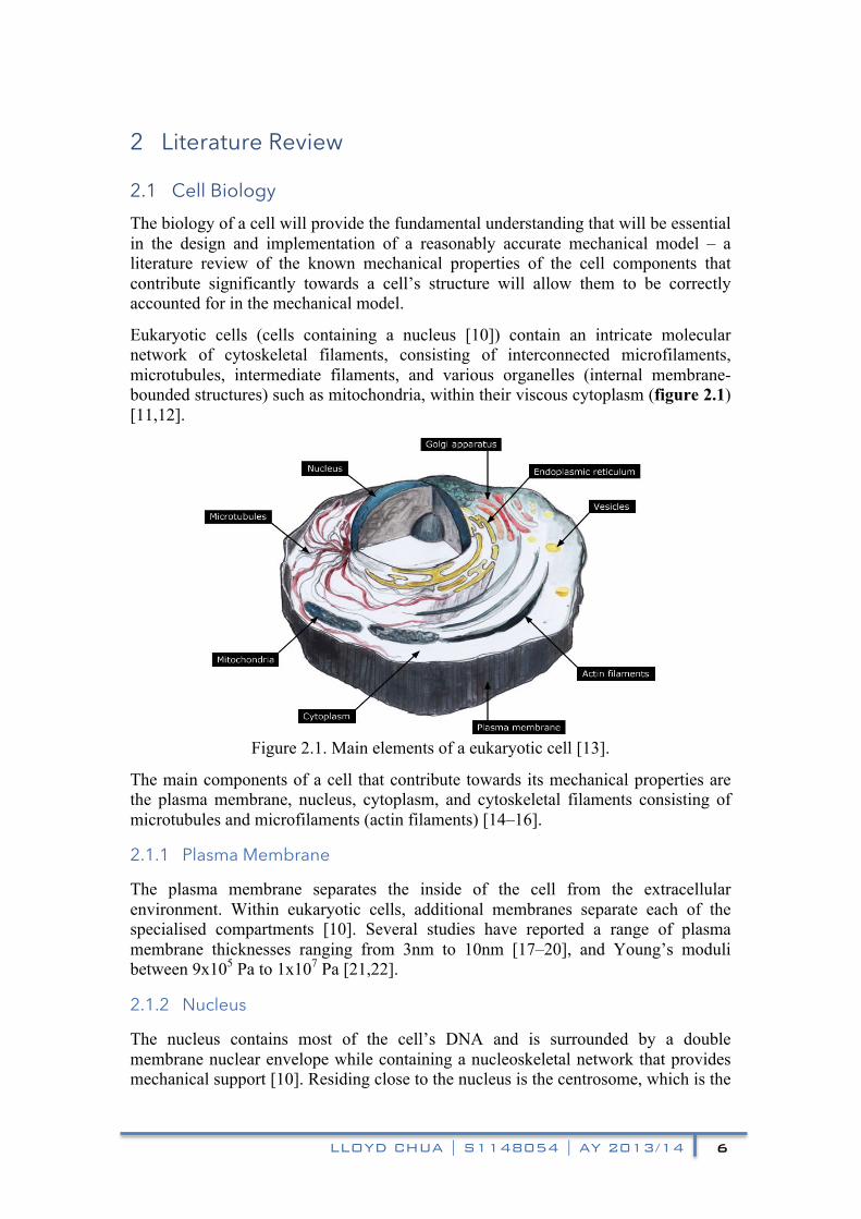
Eukaryotic cells (cells containing a nucleus [10]) contain an intricate molecular network of cytoskeletal filaments, consisting of interconnected microfilaments, microtubules, intermediate filaments, and various organelles (internal membrane-bounded structures) such as mitochondria, within their viscous cytoplasm (figure 2.1) [11,12].

Figure 2.1. Main elements of a eukaryotic cell [13].

The main components of a cell that contribute towards its mechanical properties are the plasma membrane, nucleus, cytoplasm, and cytoskeletal filaments consisting of microtubules and microfilaments (actin filaments) [14–16].

2.1.1 Plasma Membrane

The plasma membrane separates the inside of the cell from the extracellular environment. Within eukaryotic cells, additional membranes separate each of the specialised compartments [10]. Several studies have reported a range of plasma membrane thicknesses ranging from 3nm to 10nm [17–20], and Young’s moduli between 9x105 Pa to 1x107 Pa [21,22].

2.1.2 Nucleus

The nucleus contains most of the cell’s DNA and is surrounded by a double membrane nuclear envelope while containing a nucleoskeletal network that provides mechanical support [10]. Residing close to the nucleus is the centrosome, which is the

LLOYD CHUA | S1148054 | AY 2013/14 7

most common form of microtubule organising centre (MTOC) in cells where microtubule growth originates (figure 2.2) [23].

Figure 2.2. Immunofluorescence image of a cell depicting the centrosome (green

stain), the microtubule network (red stain), and the nucleus (blue stain) [13].

Studies have reported approximate values of the Young’s modulus of cell nuclei to range between 1000 Pa to 5000 Pa [24,25]. It is also noted that the relative sizes of the nucleus to the rest of the cell varied depending on the cell type, which implies that it should be a configurable parameter within the model.

2.1.3 Cytoskeleton

The cytoskeleton consists three main types of protein polymers that are strung together to produce the cytoskeletal filaments – microfilaments (actin filaments), intermediate filaments, and microtubules [10]. The cytoskeletal filaments are contained within the cell’s cytoplasm and they interact with the cellular membrane to generate and resist mechanical loads, helping to maintain the cell’s shape and structure [26].

From figures 2.3 and 2.4, microtubules (left) appear curved in form, originating from the centrosome. Microfilaments (centre) appear more linear, forming long stress fibres that span the underlying surface of the plasma membrane. Intermediate filaments (right) appear as a reticulated network that extends from the plasma membrane towards the nucleus [26].

Figure 2.3. Illustrations of the cytoskeletal structures – microtubules (left/green),

microfilaments (centre/red), and intermediate filaments (right/blue) [27].

LLOYD CHUA | S1148054 | AY 2013/14 8

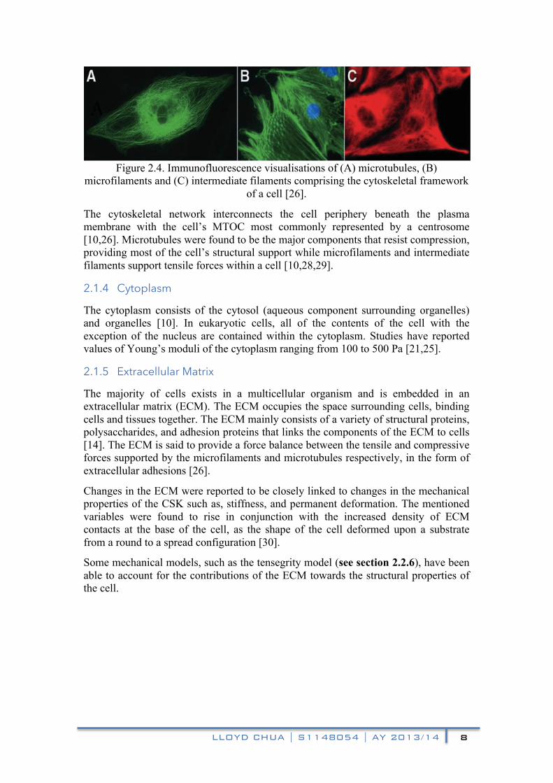
Figure 2.4. Immunofluorescence visualisations of (A) microtubules, (B)

microfilaments and (C) intermediate filaments comprising the cytoskeletal framework of a cell [26].

The cytoskeletal network interconnects the cell periphery beneath the plasma membrane with the cell’s MTOC most commonly represented by a centrosome [10,26]. Microtubules were found to be the major components that resist compression, providing most of the cell’s structural support while microfilaments and intermediate filaments support tensile forces within a cell [10,28,29].

2.1.4 Cytoplasm

The cytoplasm consists of the cytosol (aqueous component surrounding organelles) and organelles [10]. In eukaryotic cells, all of the contents of the cell with the exception of the nucleus are contained within the cytoplasm. Studies have reported values of Young’s moduli of the cytoplasm ranging from 100 to 500 Pa [21,25].

2.1.5 Extracellular Matrix

The majority of cells exists in a multicellular organism and is embedded in an extracellular matrix (ECM). The ECM occupies the space surrounding cells, binding cells and tissues together. The ECM mainly consists of a variety of structural proteins, polysaccharides, and adhesion proteins that links the components of the ECM to cells [14]. The ECM is said to provide a force balance between the tensile and compressive forces supported by the microfilaments and microtubules respectively, in the form of extracellular adhesions [26].

Changes in the ECM were reported to be closely linked to changes in the mechanical properties of the CSK such as, stiffness, and permanent deformation. The mentioned variables were found to rise in conjunction with the increased density of ECM contacts at the base of the cell, as the shape of the cell deformed upon a substrate from a round to a spread configuration [30].

Some mechanical models, such as the tensegrity model (see section 2.2.6), have been able to account for the contributions of the ECM towards the structural properties of the cell.

LLOYD CHUA | S1148054 | AY 2013/14 9

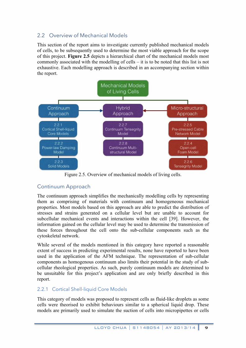
2.2 Overview of Mechanical Models This section of the report aims to investigate currently published mechanical models of cells, to be subsequently used to determine the most viable approach for the scope of this project. Figure 2.5 depicts a hierarchical chart of the mechanical models most commonly associated with the modelling of cells – it is to be noted that this list is not exhaustive. Each modelling approach is described in an accompanying section within the report.

Figure 2.5. Overview of mechanical models of living cells.

Continuum Approach The continuum approach simplifies the mechanically modelling cells by representing them as comprising of materials with continuum and homogeneous mechanical properties. Most models based on this approach are able to predict the distribution of stresses and strains generated on a cellular level but are unable to account for subcellular mechanical events and interactions within the cell [39]. However, the information gained on the cellular level may be used to determine the transmission of these forces throughout the cell onto the sub-cellular components such as the cytoskeletal network.

While several of the models mentioned in this category have reported a reasonable extent of success in predicting experimental results, none have reported to have been used in the application of the AFM technique. The representation of sub-cellular components as homogenous continuum also limits their potential in the study of sub-cellular rheological properties. As such, purely continuum models are determined to be unsuitable for this project’s application and are only briefly described in this report.

2.2.1 Cortical Shell-liquid Core Models

This category of models was proposed to represent cells as fluid-like droplets as some cells were theorised to exhibit behaviours similar to a spherical liquid drop. These models are primarily used to simulate the suction of cells into micropipettes or cells

LLOYD CHUA | S1148054 | AY 2013/14 10

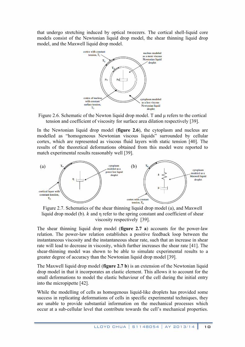
that undergo stretching induced by optical tweezers. The cortical shell-liquid core models consist of the Newtonian liquid drop model, the shear thinning liquid drop model, and the Maxwell liquid drop model.

Figure 2.6. Schematic of the Newton liquid drop model. T and µ refers to the cortical

tension and coefficient of viscosity for surface area dilation respectively [39].

In the Newtonian liquid drop model (figure 2.6), the cytoplasm and nucleus are modelled as “homogeneous Newtonian viscous liquids” surrounded by cellular cortex, which are represented as viscous fluid layers with static tension [40]. The results of the theoretical deformations obtained from this model were reported to match experimental results reasonably well [39].

Figure 2.7. Schematics of the shear thinning liquid drop model (a), and Maxwell

liquid drop model (b). ! and η refer to the spring constant and coefficient of shear viscosity respectively [39].

The shear thinning liquid drop model (figure 2.7 a) accounts for the power-law relation. The power-law relation establishes a positive feedback loop between the instantaneous viscosity and the instantaneous shear rate, such that an increase in shear rate will lead to decrease in viscosity, which further increases the shear rate [41]. The shear-thinning model was shown to be able to simulate experimental results to a greater degree of accuracy than the Newtonian liquid drop model [39].

The Maxwell liquid drop model (figure 2.7 b) is an extension of the Newtonian liquid drop model in that it incorporates an elastic element. This allows it to account for the small deformations to model the elastic behaviour of the cell during the initial entry into the micropipette [42].

While the modelling of cells as homogenous liquid-like droplets has provided some success in replicating deformations of cells in specific experimental techniques, they are unable to provide substantial information on the mechanical processes which occur at a sub-cellular level that contribute towards the cell’s mechanical properties.

(a) (b)

LLOYD CHUA | S1148054 | AY 2013/14 11

The mechanical contributions from the cytoskeletal filaments and the extracellular matrix are a couple of such examples of sub-cellular mechanical processes. These models do not allow for the analysis of these sub-cellular components that have been attributed as key mechanisms in cell compressibility [43].

2.2.2 Power-law Damping Model

The power-law damping model was proposed to better model the rheological behaviour of cells adherent on a substrate as compared to the cortical shell-liquid core models as the latter was found to overestimate the frequency dependence within cells. This model suggests that cells have mechanical properties like that of soft glassy materials near the glass transition temperature [44,45].

As cells are frequently subjected to constantly changing forces in their natural environment, this model is suitable when the dynamic behaviour of cells is of particular interest. However, the replication of the static AFM experimental results does not require the model to account for dynamic time-dependent behaviour, which renders this approach unsuitable for this project’s application.

2.2.3 Solid Models

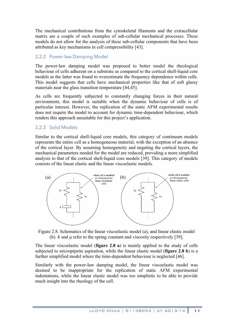
Similar to the cortical shell-liquid core models, this category of continuum models represents the entire cell as a homogeneous material, with the exception of an absence of the cortical layer. By assuming homogeneity and negating the cortical layers, the mechanical parameters needed for the model are reduced, providing a more simplified analysis to that of the cortical shell-liquid core models [39]. This category of models consists of the linear elastic and the linear viscoelastic models.

Figure 2.8. Schematics of the linear viscoelastic model (a), and linear elastic model

(b). ! and µ refer to the spring constant and viscosity respectively [39].

The linear viscoelastic model (figure 2.8 a) is mainly applied to the study of cells subjected to micropipette aspiration, while the linear elastic model (figure 2.8 b) is a further simplified model where the time-dependent behaviour is neglected [46].

Similarly with the power-law damping model, the linear viscoelastic model was deemed to be inappropriate for the replication of static AFM experimental indentations, while the linear elastic model was too simplistic to be able to provide much insight into the rheology of the cell.

(a) (b)

LLOYD CHUA | S1148054 | AY 2013/14 12

Microstructural Approach Models in the microstructural approach attempt to model the cell as a network of beam and truss elements that represent the cytoskeleton as the main structural component. These models were proposed particularly for the investigation of the cytoskeletal mechanics in cells adherent on a substrate [39].

2.2.4 Open-cell Foam Model

The open-cell foam model comprises networks of interconnected elastic struts to simulate the contribution of the cytoskeletal network towards the mechanical behaviour of cells (figure 2.9) [36,43]. The elastic structure bends as forces are applied onto the ends of the struts, simulating the deformation of a cell.

Figure 2.9. Schematic of an open-cell foam model (left) and an equivalent model undergoing deformation (right). Axial loads (F) are applied to the top and bottom

ends of struts to produce bending in the horizontally aligned beams [36].

This approach of models have produced estimated values of Young’s moduli ranging from the order of 103 Pa to 104 Pa, and the model was reported to predict experimental values obtained from micro-plate manipulation, but underestimated and overestimated values obtained from AFM and micropipette aspiration respectively [43].

The representation of the cell as a rigid interconnected structure of struts which bear the compression forces applied onto the cell does not readily correspond with what is known about the structure of the cell – the microtubules which provide the majority of a cell’s resistance to compression are not extensively interconnected and the connections between microfilaments are cross-linked rather than rigid.

2.2.5 Pre-stressed Cable Network Model

The planar pre-stressed cable network model was proposed to aid in the analysis of the mechanisms by which the cytoskeletal actin microfilaments contribute toward the mechanical properties of a cell [47,48]. As such, the model does not account for the mechanical contributions from other cellular components such as the plasma membrane, microtubules, and cytoplasm. The initial tension of the microfilaments represented by the cables in cable network models determine the mechanical response of the cell (figure 2.10), in contrast with the bending of struts in open-cell foam models [43].

LLOYD CHUA | S1148054 | AY 2013/14 13

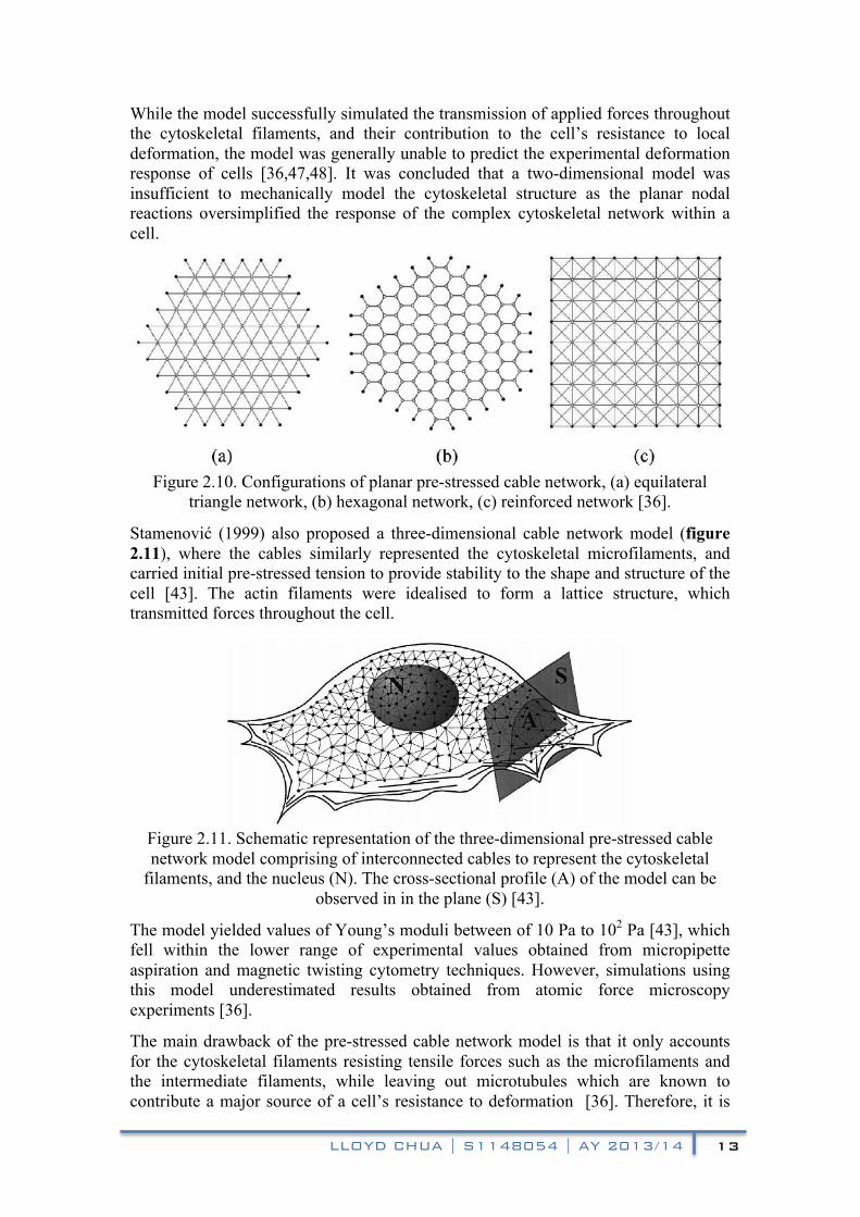
While the model successfully simulated the transmission of applied forces throughout the cytoskeletal filaments, and their contribution to the cell’s resistance to local deformation, the model was generally unable to predict the experimental deformation response of cells [36,47,48]. It was concluded that a two-dimensional model was insufficient to mechanically model the cytoskeletal structure as the planar nodal reactions oversimplified the response of the complex cytoskeletal network within a cell.

Figure 2.10. Configurations of planar pre-stressed cable network, (a) equilateral

triangle network, (b) hexagonal network, (c) reinforced network [36].

Stamenović (1999) also proposed a three-dimensional cable network model (figure 2.11), where the cables similarly represented the cytoskeletal microfilaments, and carried initial pre-stressed tension to provide stability to the shape and structure of the cell [43]. The actin filaments were idealised to form a lattice structure, which transmitted forces throughout the cell.

Figure 2.11. Schematic representation of the three-dimensional pre-stressed cable network model comprising of interconnected cables to represent the cytoskeletal

filaments, and the nucleus (N). The cross-sectional profile (A) of the model can be observed in in the plane (S) [43].

The model yielded values of Young’s moduli between of 10 Pa to 102 Pa [43], which fell within the lower range of experimental values obtained from micropipette aspiration and magnetic twisting cytometry techniques. However, simulations using this model underestimated results obtained from atomic force microscopy experiments [36].

The main drawback of the pre-stressed cable network model is that it only accounts for the cytoskeletal filaments resisting tensile forces such as the microfilaments and the intermediate filaments, while leaving out microtubules which are known to contribute a major source of a cell’s resistance to deformation [36]. Therefore, it is

LLOYD CHUA | S1148054 | AY 2013/14 14

necessary to integrate both tensile and compressive elements within a model for it to be more representative of a cell to provide a better understanding of cellular mechanisms.

2.2.6 Tensegrity Model

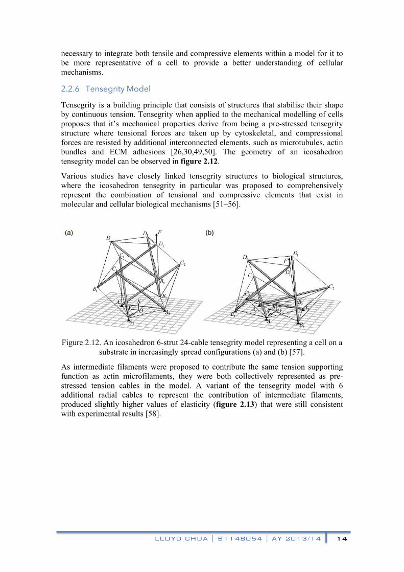
Tensegrity is a building principle that consists of structures that stabilise their shape by continuous tension. Tensegrity when applied to the mechanical modelling of cells proposes that it’s mechanical properties derive from being a pre-stressed tensegrity structure where tensional forces are taken up by cytoskeletal, and compressional forces are resisted by additional interconnected elements, such as microtubules, actin bundles and ECM adhesions [26,30,49,50]. The geometry of an icosahedron tensegrity model can be observed in figure 2.12.

Various studies have closely linked tensegrity structures to biological structures, where the icosahedron tensegrity in particular was proposed to comprehensively represent the combination of tensional and compressive elements that exist in molecular and cellular biological mechanisms [51–56].

Figure 2.12. An icosahedron 6-strut 24-cable tensegrity model representing a cell on a

substrate in increasingly spread configurations (a) and (b) [57].

As intermediate filaments were proposed to contribute the same tension supporting function as actin microfilaments, they were both collectively represented as pre-stressed tension cables in the model. A variant of the tensegrity model with 6 additional radial cables to represent the contribution of intermediate filaments, produced slightly higher values of elasticity (figure 2.13) that were still consistent with experimental results [58].

LLOYD CHUA | S1148054 | AY 2013/14 15

Figure 2.13. A 6-strut 24-cable tensegrity model with 8 additional radial cables OA,

OB, and OC representing the intermediate filaments [58].

The tensegrity model has been widely agreed upon to accurately represent cytoskeletal mechanical behaviour - studies have also reported the tensegrity model’s success in replicating experimental results of Young’s moduli and various cell behaviours such has a nonlinear increase in stiffness with increased deformation and traction forces exerted on the ECM when microtubules are disrupted [26,36,43,50,56,59].

While the tensegrity model represents large collective cross-sections of cytoskeletal filaments using a relatively limited number of struts and cables, it has been reported to accurately simulate the cellular-scale deformations (such as in hydrodynamic shearing). However, it remains to be seen as to whether the tensegrity model is suitable for small and local deformations of a cell, such as in the replication of AFM indentation techniques. It potentially implies that there may be a high variance in stiffness measurements dependent on the location of indentation, where an indentation closer to a strut/cable vertex would generate much higher values of elasticity than expected.

As such, any variation of the cytoskeletal properties may not provide meaningful results – a parametric increase in the density of the cytoskeletal filaments within the model would manifest in an increased cross-sectional area of the struts and cables, which would further concentrate the stiffness of the elements at the vertices. However, it is possible that continuum elements that represent other sub-cellular components (such as the cytoplasm and plasma membrane) may be sufficiently effective in transmitting forces to an underlying tensegrity structure if they are used in unison.

Therefore, an integration of a tensegrity structure (which represents the cytoskeletal sub-cellular mechanical responses) with continuum elements (which provides a method of distributing cellular forces to the sub-cellular cytoskeletal network) in a hybrid model is expected to be able to sufficiently simulate the experimental AFM technique.

LLOYD CHUA | S1148054 | AY 2013/14 16

Hybrid Approach This approach is based on developing a more comprehensive relationship between the continuum regions and microstructural elements of a cell. This allows the models to transmit the forces that have been induced onto the cell’s surface onto the cytoskeletal structures, integrating the principles used in continuum and microstructural models using Finite Element Analysis (FEA).

2.2.7 Finite Continuum-Tensegrity Integration within a Finite Element Model

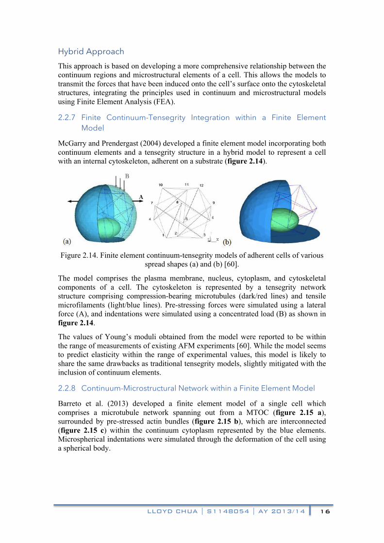
McGarry and Prendergast (2004) developed a finite element model incorporating both continuum elements and a tensegrity structure in a hybrid model to represent a cell with an internal cytoskeleton, adherent on a substrate (figure 2.14).

Figure 2.14. Finite element continuum-tensegrity models of adherent cells of various

spread shapes (a) and (b) [60].

The model comprises the plasma membrane, nucleus, cytoplasm, and cytoskeletal components of a cell. The cytoskeleton is represented by a tensegrity network structure comprising compression-bearing microtubules (dark/red lines) and tensile microfilaments (light/blue lines). Pre-stressing forces were simulated using a lateral force (A), and indentations were simulated using a concentrated load (B) as shown in figure 2.14.

The values of Young’s moduli obtained from the model were reported to be within the range of measurements of existing AFM experiments [60]. While the model seems to predict elasticity within the range of experimental values, this model is likely to share the same drawbacks as traditional tensegrity models, slightly mitigated with the inclusion of continuum elements.

2.2.8 Continuum-Microstructural Network within a Finite Element Model

Barreto et al. (2013) developed a finite element model of a single cell which comprises a microtubule network spanning out from a MTOC (figure 2.15 a), surrounded by pre-stressed actin bundles (figure 2.15 b), which are interconnected (figure 2.15 c) within the continuum cytoplasm represented by the blue elements. Microspherical indentations were simulated through the deformation of the cell using a spherical body.

LLOYD CHUA | S1148054 | AY 2013/14 17

Figure 2.15. Finite element continuum-microstructural model of a single cell.

Microtubule distribution (a), actin bundle distribution (b), and interaction between microtubules and actin bundles (c) [29].

This mechanical model is reported to be able to maintain the fundamental principles of tensegrity (pre-stressed elements providing stability). But in contrast to tensegrity-based models, the elements representing the cytoskeletal filaments are free to move independently. The study has similarly reported success in replicating experimentally obtained results.

In comparison with the continuum-tensegrity model, this approach to the modelling of the microstructure is relatively unsupported by existing literature. The method that this modelling approach has taken in determining the nodal positions of the junctions connecting the actin bundles with the microtubules appears to be arbitrary and sparse. While increasing the number of microstructural elements through additional microtubule and actin filaments can mitigate these factors, this approach is considerably more difficult to implement in a parametric model and may become excessively computationally intensive for a parametric study.

2.2.9 Summary of Literature Review

Models that constituted purely continuum or microstructural models were determined to be insufficiently robust to simulate AFM techniques or provide any further insights to a cell’s mechanical properties. To account for the “complex geometry, sliding boundary conditions and the nonlinear relations” [36] involved with the modelling of a cell, the finite-element method (FEM) provides a viable method to the modelling of cells [39]. It was determined that a finite element analysis of the continuum-tensegrity approach would produce a model that would be sufficiently effective in a parametric study of the mechanical properties of cells.

Amongst the published hybrid models that were able to predict cell elasticity within the range of experimental values, it was unclear as to which of the models provided the most accurate results. Due to the relative geometrical simplicity of the continuum-tensegrity model (see section 2.2.7) compared to the continuum-microstructural model (see section 2.2.8), it was determined that a finite element model of a continuum-tensegrity model would provide the highest likelihood of success within the project’s timeline and as such, should be the goal of the first modelling approach.

(a) (b) (c)

LLOYD CHUA | S1148054 | AY 2013/14 18

3 Modelling Methodology A finite element model was implemented for the purpose of investigating the sub-cellular contributions towards a cell’s Young’s moduli. The model was primarily focused to simulate indentations for comparison with measurements obtained from AFM experiments. The axisymmetric model consists of 4 components representing sub-cellular regions of the cell known to be major contributors towards a cell’s stiffness; a nucleus, a cytoplasmic region, and an enveloping plasma membrane connected with a tensegrity structure.

The nucleus and cytoplasm were meshed using tetrahedral elements, and the plasma membrane was meshed using shell tetrahedral elements. The icosahedron tensegrity network representing the microtubules and microfilaments was meshed using T3D2 truss elements. To simulate the force distribution within the tensegrity structure, the tensional forces within the microtubule struts as well as the compressive forces within the microfilament cables were disabled.

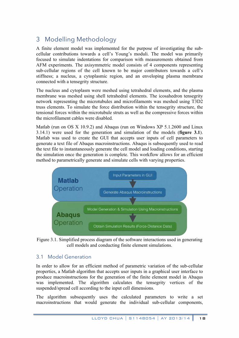
Matlab (run on OS X 10.9.2) and Abaqus (run on Windows XP 5.1.2600 and Linux 3.14.1) were used for the generation and simulation of the models (figure 3.1). Matlab was used to create the GUI that accepts user inputs of cell parameters to generate a text file of Abaqus macroinstructions. Abaqus is subsequently used to read the text file to instantaneously generate the cell model and loading conditions, starting the simulation once the generation is complete. This workflow allows for an efficient method to parametrically generate and simulate cells with varying properties.

Figure 3.1. Simplified process diagram of the software interactions used in generating

cell models and conducting finite element simulations.

3.1 Model Generation In order to allow for an efficient method of parametric variation of the sub-cellular properties, a Matlab algorithm that accepts user inputs in a graphical user interface to produce macroinstructions for the generation of the finite element model in Abaqus was implemented. The algorithm calculates the tensegrity vertices of the suspended/spread cell according to the input cell dimensions.

The algorithm subsequently uses the calculated parameters to write a set macroinstructions that would generate the individual sub-cellular components,

LLOYD CHUA | S1148054 | AY 2013/14 19

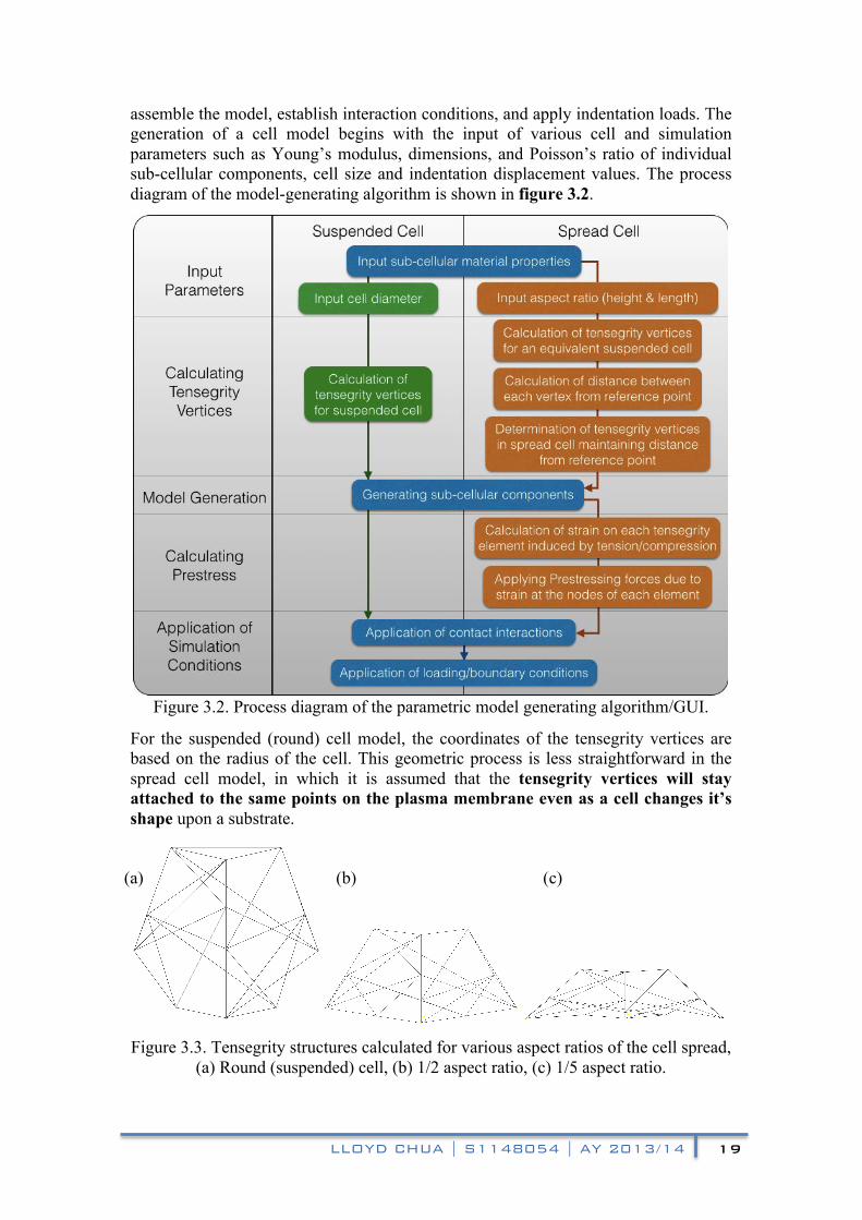
assemble the model, establish interaction conditions, and apply indentation loads. The generation of a cell model begins with the input of various cell and simulation parameters such as Young’s modulus, dimensions, and Poisson’s ratio of individual sub-cellular components, cell size and indentation displacement values. The process diagram of the model-generating algorithm is shown in figure 3.2.

Figure 3.2. Process diagram of the parametric model generating algorithm/GUI.

For the suspended (round) cell model, the coordinates of the tensegrity vertices are based on the radius of the cell. This geometric process is less straightforward in the spread cell model, in which it is assumed that the tensegrity vertices will stay attached to the same points on the plasma membrane even as a cell changes it’s shape upon a substrate.

Figure 3.3. Tensegrity structures calculated for various aspect ratios of the cell spread,

(a) Round (suspended) cell, (b) 1/2 aspect ratio, (c) 1/5 aspect ratio.

(a) (b) (c)

LLOYD CHUA | S1148054 | AY 2013/14 20

As such, the algorithm firstly calculates the tensegrity vertices of a suspended cell of an equivalent circumference. It then calculates the arc length (distance along the plasma membrane) to each vertex from a reference point on the equivalent suspended cell. Maintaining the arc lengths from the suspended cell, the tensegrity vertices are then determined for the spread cell. Figure 3.3 depicts the tensegrity structures that are generated by the algorithm at various cell aspect ratios.!

3.2 Pre-stressing The tensegrity structure was hypothesized to increase pre-stress as the cell increases it’s spread and induces forces on the structure. From figure 3.3 (a), (b), and (c), it can be observed that some elements within the tensegrity structure are compressed and shortened, while others are elongated as the cell spreads in attempt to maintain the tensegrity vertices on the membrane. This pre-stress is calculated by using the original and new lengths of each element to calculate the strain experienced. The calculated strain values are then converted to nodal forces at the two ends of each element using the input Young’s modulus and cross-sectional area of each element. The forces contributed by individual elements at each vertex are then converted to force vectors that are applied on each of the tensegrity vertices (figure 3.4).

Figure 3.4. Pre-stressing force vectors (yellow) calculated and applied at tensegrity

vertices.

However, it was found that the large number of forces applied on the model as the result of the pre-stress were incompatible with the non-linear simulations required by the rigid body indenters. As such, the pre-stressing setting is only enabled for point loading conditions and the analysis of these simulations are not included in this report.

LLOYD CHUA | S1148054 | AY 2013/14 21

3.3 Loading Conditions The model was tested using 4 types of indentation conditions namely, point loading (only usable to determine stiffness and not Young’s modulus), spherical, cylindrical, and conical indentations. As the conical indentations were subsequently determined to be unsuitable for the model (see section 4.1), only the first 3 indentation conditions were included in the model generator. The following are the theoretical contact mechanics equations used to convert the force-distance data obtained from the simulations into values of local Young’s moduli of the cell model.

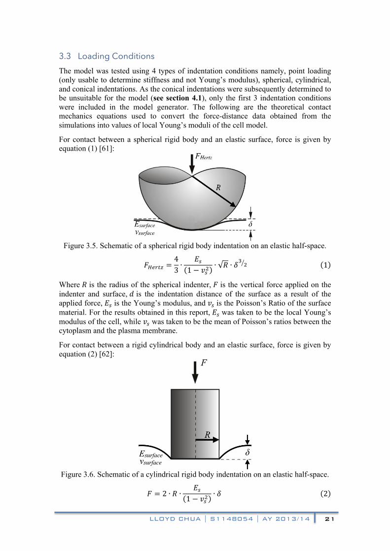
For contact between a spherical rigid body and an elastic surface, force is given by equation (1) [61]:

Figure 3.5. Schematic of a spherical rigid body indentation on an elastic half-space.

!!"#$% =43 ∙

!!1− !!!

∙ ! ∙ !! !!!!!!!!!!!!!!!!!!!!!!!!!!!!!!!!!!!!!!!!!!! 1

Where ! is the radius of the spherical indenter, ! is the vertical force applied on the indenter and surface, ! is the indentation distance of the surface as a result of the applied force, !! is the Young’s modulus, and !! is the Poisson’s Ratio of the surface material. For the results obtained in this report, !! was taken to be the local Young’s modulus of the cell, while !! was taken to be the mean of Poisson’s ratios between the cytoplasm and the plasma membrane.

For contact between a rigid cylindrical body and an elastic surface, force is given by equation (2) [62]:

Figure 3.6. Schematic of a cylindrical rigid body indentation on an elastic half-space.

! = 2 ∙ ! ∙ !!1− !!!

∙ !!!!!!!!!!!!!!!!!!!!!!!!!!!!!!!!!!!!!!!!!!!!!!!!!!!!!!!!!! 2

LLOYD CHUA | S1148054 | AY 2013/14 22

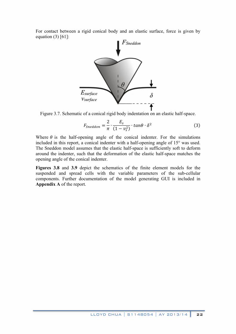
For contact between a rigid conical body and an elastic surface, force is given by equation (3) [61]:

Figure 3.7. Schematic of a conical rigid body indentation on an elastic half-space.

!!"#$$%" =2! ∙

!!1− !!!

∙ !"#$ ∙ !!!!!!!!!!!!!!!!!!!!!!!!!!!!!!!!!!!!!!!!!! 3

Where ! is the half-opening angle of the conical indenter. For the simulations included in this report, a conical indenter with a half-opening angle of 15° was used. The Sneddon model assumes that the elastic half-space is sufficiently soft to deform around the indenter, such that the deformation of the elastic half-space matches the opening angle of the conical indenter.

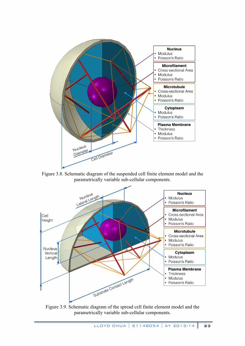
Figures 3.8 and 3.9 depict the schematics of the finite element models for the suspended and spread cells with the variable parameters of the sub-cellular components. Further documentation of the model generating GUI is included in Appendix A of the report.

LLOYD CHUA | S1148054 | AY 2013/14 23

Figure 3.8. Schematic diagram of the suspended cell finite element model and the

parametrically variable sub-cellular components.

Figure 3.9. Schematic diagram of the spread cell finite element model and the

parametrically variable sub-cellular components.

LLOYD CHUA | S1148054 | AY 2013/14 24

4 Simulation Results and Analysis

4.1 Model Validation: Comparison with Experimental Measurements

4.1.1 Modelling an Endothelial Cell

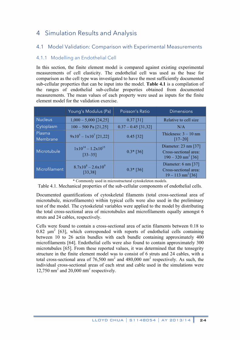
In this section, the finite element model is compared against existing experimental measurements of cell elasticity. The endothelial cell was used as the base for comparison as the cell type was investigated to have the most sufficiently documented sub-cellular properties that can be input into the model. Table 4.1 is a compilation of the ranges of endothelial sub-cellular properties obtained from documented measurements. The mean values of each property were used as inputs for the finite element model for the validation exercise.

Young’s Modulus (Pa) Poisson’s Ratio Dimensions

Nucleus 1,000 – 5,000 [24,25] 0.37 [31] Relative to cell size Cytoplasm 100 – 500 Pa [21,25] 0.37 – 0.45 [31,32] N/A Plasma Membrane

9x105 – 1x107 [21,22] 0.45 [32] Thickness: 3 – 10 nm [17–20]

Microtubule 1x1014 – 1.2x1015

[33–35] 0.3* [36]

Diameter: 23 nm [37] Cross-sectional area: 190 – 320 nm2 [36]

Microfilament 8.7x108 – 2.6x109 [33,38] 0.3* [36]

Diameter: 6 nm [37] Cross-sectional area:

19 – 113 nm2 [36] * Commonly used in microstructural cytoskeleton models.

Table 4.1. Mechanical properties of the sub-cellular components of endothelial cells.

Documented quantifications of cytoskeletal filaments (total cross-sectional area of microtubule, microfilaments) within typical cells were also used in the preliminary test of the model. The cytoskeletal variables were applied to the model by distributing the total cross-sectional area of microtubules and microfilaments equally amongst 6 struts and 24 cables, respectively.

Cells were found to contain a cross-sectional area of actin filaments between 0.18 to 0.82 µm2 [63], which corresponded with reports of endothelial cells containing between 10 to 26 actin bundles with each bundle containing approximately 400 microfilaments [64]. Endothelial cells were also found to contain approximately 300 microtubules [65]. From these reported values, it was determined that the tensegrity structure in the finite element model was to consist of 6 struts and 24 cables, with a total cross-sectional area of 76,500 nm2 and 480,000 nm2 respectively. As such, the individual cross-sectional areas of each strut and cable used in the simulations were 12,750 nm2 and 20,000 nm2 respectively.

LLOYD CHUA | S1148054 | AY 2013/14 25

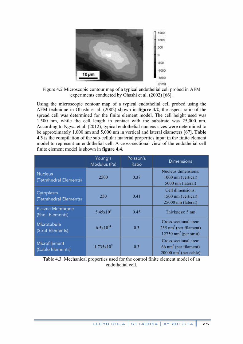
Figure 4.2 Microscopic contour map of a typical endothelial cell probed in AFM

experiments conducted by Ohashi et al. (2002) [66].

Using the microscopic contour map of a typical endothelial cell probed using the AFM technique in Ohashi et al. (2002) shown in figure 4.2, the aspect ratio of the spread cell was determined for the finite element model. The cell height used was 1,500 nm, while the cell length in contact with the substrate was 25,000 nm. According to Ngwa et al. (2012), typical endothelial nucleus sizes were determined to be approximately 1,000 nm and 5,000 nm in vertical and lateral diameters [67]. Table 4.3 is the compilation of the sub-cellular material properties input in the finite element model to represent an endothelial cell. A cross-sectional view of the endothelial cell finite element model is shown in figure 4.4.

Young’s Modulus (Pa)

Poisson’s Ratio

Dimensions

Nucleus (Tetrahedral Elements)

2500 0.37 Nucleus dimensions: 1000 nm (vertical) 5000 nm (lateral)

Cytoplasm (Tetrahedral Elements)

250 0.41 Cell dimensions:

1500 nm (vertical) 25000 nm (lateral)

Plasma Membrane (Shell Elements)

5.45x106 0.45 Thickness: 5 nm

Microtubule (Strut Elements)

6.5x1014 0.3 Cross-sectional area:

255 nm2 (per filament) 12750 nm2 (per strut)

Microfilament (Cable Elements)

1.735x109 0.3 Cross-sectional area: 66 nm2 (per filament) 20000 nm2 (per cable)

Table 4.3. Mechanical properties used for the control finite element model of an endothelial cell.

LLOYD CHUA | S1148054 | AY 2013/14 26

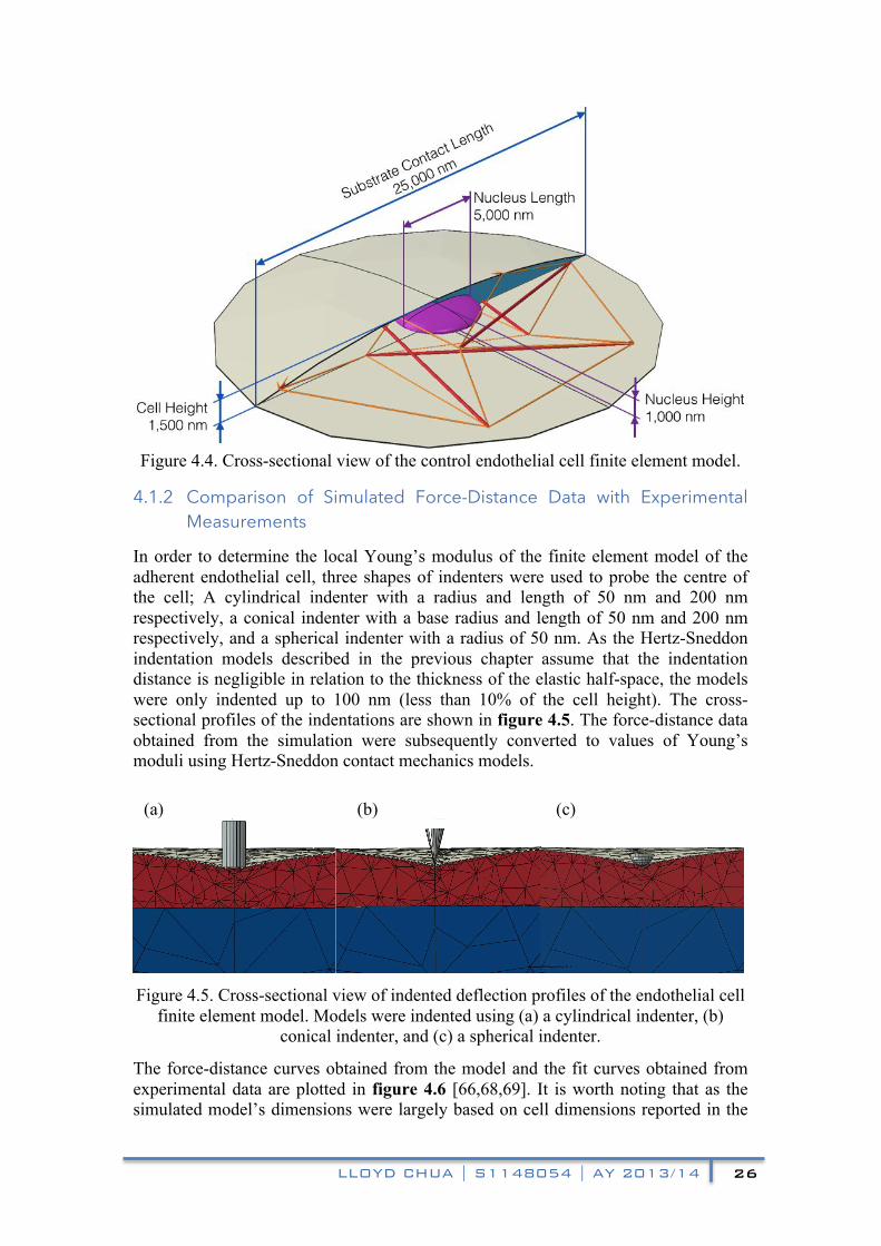
Figure 4.4. Cross-sectional view of the control endothelial cell finite element model.

4.1.2 Comparison of Simulated Force-Distance Data with Experimental Measurements

In order to determine the local Young’s modulus of the finite element model of the adherent endothelial cell, three shapes of indenters were used to probe the centre of the cell; A cylindrical indenter with a radius and length of 50 nm and 200 nm respectively, a conical indenter with a base radius and length of 50 nm and 200 nm respectively, and a spherical indenter with a radius of 50 nm. As the Hertz-Sneddon indentation models described in the previous chapter assume that the indentation distance is negligible in relation to the thickness of the elastic half-space, the models were only indented up to 100 nm (less than 10% of the cell height). The cross-sectional profiles of the indentations are shown in figure 4.5. The force-distance data obtained from the simulation were subsequently converted to values of Young’s moduli using Hertz-Sneddon contact mechanics models.

Figure 4.5. Cross-sectional view of indented deflection profiles of the endothelial cell

finite element model. Models were indented using (a) a cylindrical indenter, (b) conical indenter, and (c) a spherical indenter.

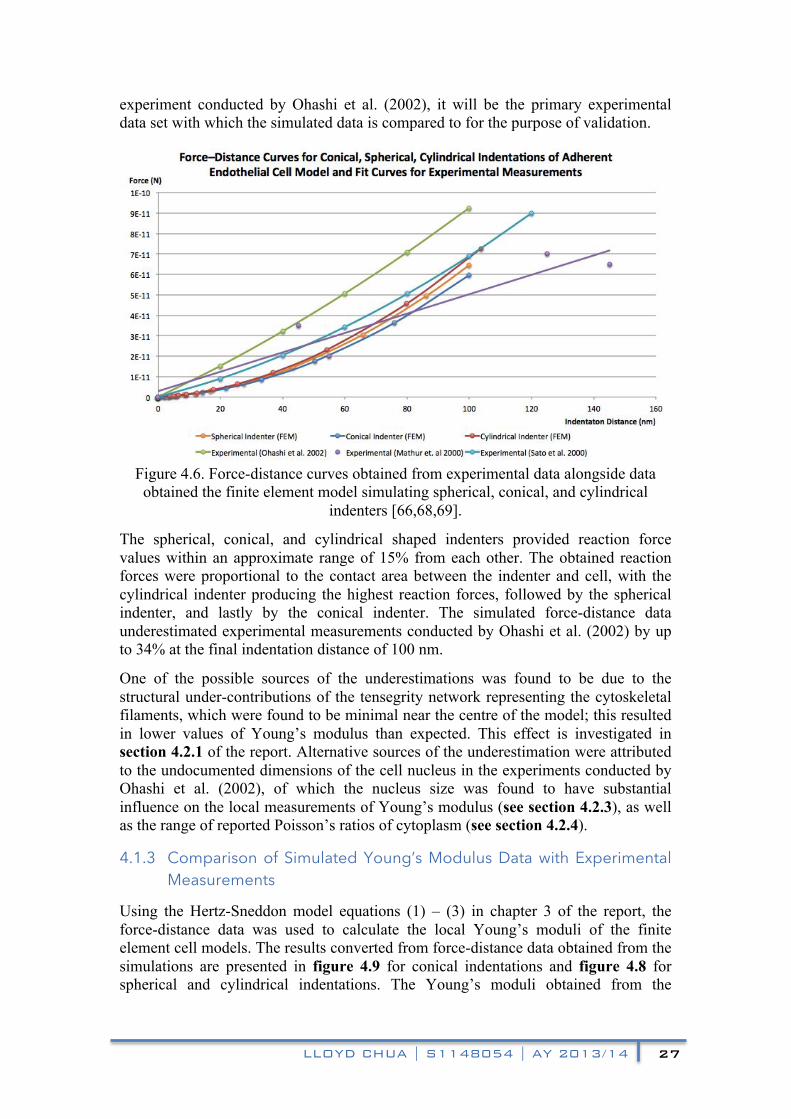
The force-distance curves obtained from the model and the fit curves obtained from experimental data are plotted in figure 4.6 [66,68,69]. It is worth noting that as the simulated model’s dimensions were largely based on cell dimensions reported in the

(a) (b) (c)

LLOYD CHUA | S1148054 | AY 2013/14 27

experiment conducted by Ohashi et al. (2002), it will be the primary experimental data set with which the simulated data is compared to for the purpose of validation.

Figure 4.6. Force-distance curves obtained from experimental data alongside data obtained the finite element model simulating spherical, conical, and cylindrical

indenters [66,68,69].

The spherical, conical, and cylindrical shaped indenters provided reaction force values within an approximate range of 15% from each other. The obtained reaction forces were proportional to the contact area between the indenter and cell, with the cylindrical indenter producing the highest reaction forces, followed by the spherical indenter, and lastly by the conical indenter. The simulated force-distance data underestimated experimental measurements conducted by Ohashi et al. (2002) by up to 34% at the final indentation distance of 100 nm.

One of the possible sources of the underestimations was found to be due to the structural under-contributions of the tensegrity network representing the cytoskeletal filaments, which were found to be minimal near the centre of the model; this resulted in lower values of Young’s modulus than expected. This effect is investigated in section 4.2.1 of the report. Alternative sources of the underestimation were attributed to the undocumented dimensions of the cell nucleus in the experiments conducted by Ohashi et al. (2002), of which the nucleus size was found to have substantial influence on the local measurements of Young’s modulus (see section 4.2.3), as well as the range of reported Poisson’s ratios of cytoplasm (see section 4.2.4).

4.1.3 Comparison of Simulated Young’s Modulus Data with Experimental Measurements

Using the Hertz-Sneddon model equations (1) – (3) in chapter 3 of the report, the force-distance data was used to calculate the local Young’s moduli of the finite element cell models. The results converted from force-distance data obtained from the simulations are presented in figure 4.9 for conical indentations and figure 4.8 for spherical and cylindrical indentations. The Young’s moduli obtained from the

LLOYD CHUA | S1148054 | AY 2013/14 28

simulated models were compared to the experimentally derived Young’s moduli and are tabulated in table 4.7.

Data Source Young’s Modulus (kPa)

Sato et al. (2004) 10 – 11 Mathur et al. (2000) 1.3 – 7.2 Ohashi et al. (2002) 0.9 – 1.7 Pesen and Ho (2005) 0.2 – 2.0 Spherical Indenter (0 – 100 nm)

3.6 – 6.8 (Stable)

Cylindrical Indenter (0 – 100 nm)

1.6 – 8.7 (Increases with further indentation)

Conical Indenter (0 – 100 nm)

280 – 30 (Decreases with further indentation)

Table 4.7. Experimental AFM measurements of the Young’s modulus of endothelial cells [61].

From table 4.7, it can be observed that all 3 indentations provided overestimated values of Young’s modulus as compared to measurements reported by Ohashi et al. (2002), while only the spherical and cylindrical indentations provided estimates of Young’s modulus within the range of experimentally reported values of 0.2 to 11 kPa. The spherical indenter provided the smallest range of values of Young’s moduli from 3.6 to 6.8 kPa that stabilises with further indentation (figure 4.8). The cylindrical indenter provided a range from 1.6 to 8.7 kPa that increases with further indentation (figure 4.8). The conical indenter provided a range from 280 to 30 kPa that decreases with further indentation (figure 4.9). It is worth noting that Ohashi et al. (2002) had utilised the conical contact equation to convert their force-distance curve obtained from a pyramidal indenter used in their experiments. As such, the Young’s modulus values obtained from their experiments might be subjected to significant errors.

Figure 4.8. Local Young’s modulus data for spherical and cylindrical indentation

simulations of the endothelial cell.

LLOYD CHUA | S1148054 | AY 2013/14 29

Figure 4.9. Local Young’s modulus data for conical indentation simulations of the

endothelial cell.

4.1.4 Determining the Ideal Indenter Shape for the Parametric Variation Simulations

For the simulations of all 3 indenter shapes shown in figure 4.8 and 4.9, 2 distinct stages are observed in the modulus-distance relationship. The first stage involves a relatively high initial Young’s modulus which decays with indented distance (up to 10 nm). This is thought to be due to the artifacts of the finite element model as the indenter comes into initial contact with the cell. Another source of this effect is attributed to the higher modulus of the plasma membrane in relation to the cytoplasm. The effect of the plasma membrane may be have a predominant effect on reaction forces at smaller displacements close the membrane thickness (5 nm).

This is followed by a second stage where the Young’s modulus is seen to increase with indented distance (from 10 nm onwards) for the spherical and cylindrical indenters. However, the Young’s modulus continues to decrease for the conical indenter. The Young’s moduli obtained from the cylindrical indenter exhibits a linear relationship with the indented distance, which appears to continue to increase linearly when extrapolated beyond 100 nm. The modulus increase with indented distance for the spherical indenter appears to decay, allowing the measured Young’s modulus to stabilise as the indented distance approaches and exceeds 100 nm.

It can be observed that the Sneddon model (equation 3) used to convert force-distance data to Young’s moduli for a conical indenter produced values that were approximately 5 to 40 times higher than values obtained from the cylindrical and spherical indenter simulations, as well as the experimentally derived Young’s modulus. This effect is attributed to the fact that the Sneddon model assumes that the relatively soft elastic body deforms around the conical indenter, allowing the elastic body to match the opening angle of the indenter (figure 3.5); this soft body deformation was not observed in the model’s simulated deformation (figure 4.5 b).

From the deformation profile of the conical indentation finite element simulation, the Young’s modulus data derived from conical indenter was expected to provide overestimated values in relation to the spherical and cylindrical indenters. This result

LLOYD CHUA | S1148054 | AY 2013/14 30

implies that the conical indenter may be unsuitable for finite element simulation of cells. It also implies that conical indentations may be unsuitable for experimental indentations of certain cells as the surface properties of a cell (largely contributed by plasma membrane) may not allow for the soft body deformation required for the Sneddon model to be valid.

Between the cylindrical and spherical indenters, the spherical indenter provided an increasingly stable Young’s modulus with increasing indentation distance. A spherical indenter is also more representative of the experimental indenters. Therefore, the spherical indenter was deemed to be the most appropriate for the subsequent parametric simulations conducted in this report.

4.2 Parametric Variation of Variables

4.2.1 Influence of Indentation Location on Young’s Modulus

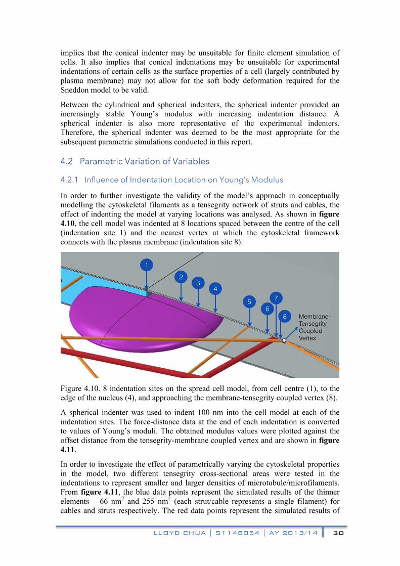
In order to further investigate the validity of the model’s approach in conceptually modelling the cytoskeletal filaments as a tensegrity network of struts and cables, the effect of indenting the model at varying locations was analysed. As shown in figure 4.10, the cell model was indented at 8 locations spaced between the centre of the cell (indentation site 1) and the nearest vertex at which the cytoskeletal framework connects with the plasma membrane (indentation site 8).

Figure 4.10. 8 indentation sites on the spread cell model, from cell centre (1), to the edge of the nucleus (4), and approaching the membrane-tensegrity coupled vertex (8).

A spherical indenter was used to indent 100 nm into the cell model at each of the indentation sites. The force-distance data at the end of each indentation is converted to values of Young’s moduli. The obtained modulus values were plotted against the offset distance from the tensegrity-membrane coupled vertex and are shown in figure 4.11.

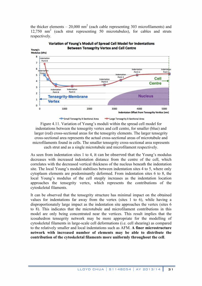
In order to investigate the effect of parametrically varying the cytoskeletal properties in the model, two different tensegrity cross-sectional areas were tested in the indentations to represent smaller and larger densities of microtubule/microfilaments. From figure 4.11, the blue data points represent the simulated results of the thinner elements – 66 nm2 and 255 nm2 (each strut/cable represents a single filament) for cables and struts respectively. The red data points represent the simulated results of

LLOYD CHUA | S1148054 | AY 2013/14 31

the thicker elements – 20,000 nm2 (each cable representing 303 microfilaments) and 12,750 nm2 (each strut representing 50 microtubules), for cables and struts respectively.!

Figure 4.11. Variation of Young’s moduli within the spread cell model for

indentations between the tensegrity vertex and cell centre, for smaller (blue) and larger (red) cross-sectional areas for the tensegrity elements. The larger tensegrity cross-sectional area represents the actual cross-sectional areas of microtubule and

microfilaments found in cells. The smaller tensegrity cross-sectional area represents each strut and as a single microtubule and microfilament respectively.

As seen from indentation sites 1 to 4, it!can!be!observed!that!the Young’s modulus decreases with increased! indentation distance from the centre of the cell, which correlates with the decreased vertical thickness of the nucleus beneath the indentation site. The local Young’s moduli stabilises between indentation sites 4 to 5, where only cytoplasm elements are predominantly deformed. From indentation sites 6 to 8, the local Young’s modulus of the cell steeply increases as the indentation location approaches the tensegrity vertex, which represents the contributions of the cytoskeletal filaments.

It can be observed that the tensegrity structure has minimal impact on the obtained values for indentations far away from the vertex (sites 1 to 6), while having a disproportionately large impact as the indentation site approaches the vertex (sites 6 to 8). This indicates that the microtubule and microfilament contributions in this model are only being concentrated near the vertices. This result implies that the icosahedron tensegrity network may be more appropriate for the modelling of cytoskeletal filaments in large-scale cell deformations (i.e. cell shearing) as compared to the relatively smaller and local indentations such as AFM. A finer microstructure network with increased number of elements may be able to distribute the contribution of the cytoskeletal filaments more uniformly throughout the cell.

LLOYD CHUA | S1148054 | AY 2013/14 32

4.2.2 Influence of Cell Aspect Ratio on Young’s Modulus

Cells are often studied while adherent on a flat substrate with most AFM measurements of cells being conducted in a similar manner. As cells continually spread from a round shape when suspended to a relatively flat shape when left over time, it is worth investigating that the influence the aspect ratio of the cell has on its overall stiffness. Keeping the volume of the cell constant, 5 models of varying aspect ratios (height/ length), 1, 1/2, 1/5, 1/10 and 1/20, were simulated with a spherical indenter of 50 nm radius as shown in figure 4.12.

Figure 4.12. Cross-sectional views of spread cell finite element models of varying

aspect ratios with constant volume – (a) 1, (b) 1/2, (c) 1/5, (d) 1/10, (e) 1/20.

From the results of the simulations (figure 4.13), it can be observed that increasing the aspect ratio (increasingly round cell) decreased the local Young’s modulus of the cell model. The effect of increasing the aspect ratio on the decreasing Young’s modulus diminishes as the cell approaches the shape that resembles a round

(a) (b)

(c) (d)

(e)

LLOYD CHUA | S1148054 | AY 2013/14 33

suspended cell. It was found that a cell of an aspect ratio of 1/20 was approximately 331.2% stiffer than an identical cell of an aspect ratio of 1.

Figure 4.13. Bar chart of the finite element cell model’s local Young’s modulus at

varying aspect ratios from 1 to 1/20.

This result implies that round suspended cells are in general, have a lower elastic modulus than similar cells that have a higher spread on a substrate. In extension, cells adherent on a substrate increase their spread over time (decreased aspect ratio) increasing their elastic modulus. The further implications of this result on the experimental measurements for the purpose of distinguishing between cell types, is that the selection of specific cells based on their spread configuration has a significant effect on the measured cell elasticity. Therefore, in the comparison of different cells, similar aspect ratios need to be considered. Possible causes of this phenomenon, such as the changing mechanical contributions of each sub-cellular component at different cell shapes are investigated section 4.2.3.

4.2.3 Varying Membrane, Cytoplasm and Nucleus Young’s Modulus

!Figure 4.14. Cross-sectional views of spread cell finite element models of varying aspect ratios with constant volume – (a) 1/5 and (b) 1/20.

The parametric variation of the sub-cellular Young’s moduli was conducted for two cell aspect ratios, 1/5 (figure 4.14 a) and 1/20 (figure 4.14 b), in an effort to isolate the source of the changing local Young’s modulus as a cell changes its shape on a

(a) (b)

LLOYD CHUA | S1148054 | AY 2013/14 34

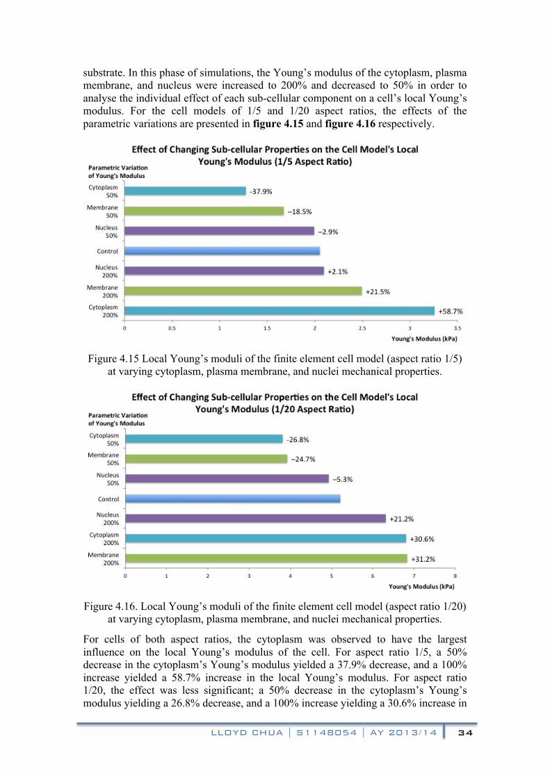
substrate. In this phase of simulations, the Young’s modulus of the cytoplasm, plasma membrane, and nucleus were increased to 200% and decreased to 50% in order to analyse the individual effect of each sub-cellular component on a cell’s local Young’s modulus. For the cell models of 1/5 and 1/20 aspect ratios, the effects of the parametric variations are presented in figure 4.15 and figure 4.16 respectively.

Figure 4.15 Local Young’s moduli of the finite element cell model (aspect ratio 1/5)

at varying cytoplasm, plasma membrane, and nuclei mechanical properties.

Figure 4.16. Local Young’s moduli of the finite element cell model (aspect ratio 1/20)

at varying cytoplasm, plasma membrane, and nuclei mechanical properties.

For cells of both aspect ratios, the cytoplasm was observed to have the largest influence on the local Young’s modulus of the cell. For aspect ratio 1/5, a 50% decrease in the cytoplasm’s Young’s modulus yielded a 37.9% decrease, and a 100% increase yielded a 58.7% increase in the local Young’s modulus. For aspect ratio 1/20, the effect was less significant; a 50% decrease in the cytoplasm’s Young’s modulus yielding a 26.8% decrease, and a 100% increase yielding a 30.6% increase in

LLOYD CHUA | S1148054 | AY 2013/14 35

the local Young’s modulus. A possible explanation for the increased influence of the cytoplasm in rounder cells is attributed to the larger region of displaced cytoplasm in the indentation of rounder cells.

The plasma membrane had the most significant influence on the cell’s local Young’s modulus after the cytoplasm. For aspect ratio 1/5, a 50% decrease in the membrane’s Young’s modulus yielded an 18.5% decrease, and a 100% increase yielded a 21.5% increase in the local Young’s modulus. For aspect ratio 1/20, a 50% decrease in the membrane’s Young’s modulus yielded a 24.7% decrease, and a 100% increase yielded a 31.2% increase in the local Young’s modulus. A larger cytoplasm influence can be observed in the rounder 1/5 aspect ratio cell, while in the 1/20 aspect ratio cell, the influence of the cytoplasm and the membrane on the local Young’s modulus were largely similar. However, in contrast with the cytoplasm, the influence of the membrane on the local Young’s modulus was proportional with the cell’s degree of spread indicating that the membrane’s increased influence was due to its increased proportion of the region displaced by the indentation.

The nucleus was observed to have the least significant influence on the local Young’s modulus in the rounder cell. For the aspect ratio 1/5, a 50% decrease and 100% increase in the nuclei’s Young’s modulus resulted in a 2.9% decrease and 2.1% increase in the local Young’s modulus respectively. However, the influence of the nucleus increased in the cell with a higher degree of spread. For the aspect ratio 1/20, a 50% decrease and 100% increase in the nuclei’s Young’s modulus resulted in a 5.3% decrease and 21.2% increase respectively. This implies that the proximity and positioning of the sub-cellular components plays a large role in influencing the Young’s modulus of the cell obtained from a local indentation. Therefore, any experimental AFM indentation of a cell for the purpose of measuring cell elasticity needs to consider the indentation site in relation to any discernible sub-cellular components such as nuclei and mitochondria.

4.2.4 Varying Cytoplasm Poisson’s Ratio

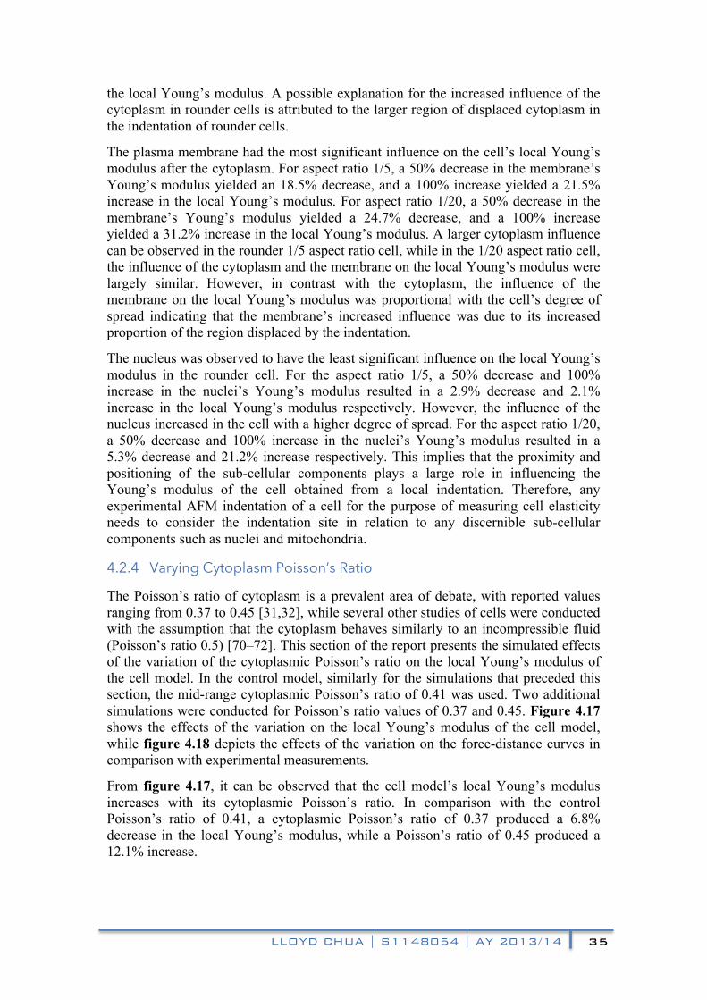
The Poisson’s ratio of cytoplasm is a prevalent area of debate, with reported values ranging from 0.37 to 0.45 [31,32], while several other studies of cells were conducted with the assumption that the cytoplasm behaves similarly to an incompressible fluid (Poisson’s ratio 0.5) [70–72]. This section of the report presents the simulated effects of the variation of the cytoplasmic Poisson’s ratio on the local Young’s modulus of the cell model. In the control model, similarly for the simulations that preceded this section, the mid-range cytoplasmic Poisson’s ratio of 0.41 was used. Two additional simulations were conducted for Poisson’s ratio values of 0.37 and 0.45. Figure 4.17 shows the effects of the variation on the local Young’s modulus of the cell model, while figure 4.18 depicts the effects of the variation on the force-distance curves in comparison with experimental measurements.

From figure 4.17, it can be observed that the cell model’s local Young’s modulus increases with its cytoplasmic Poisson’s ratio. In comparison with the control Poisson’s ratio of 0.41, a cytoplasmic Poisson’s ratio of 0.37 produced a 6.8% decrease in the local Young’s modulus, while a Poisson’s ratio of 0.45 produced a 12.1% increase.

LLOYD CHUA | S1148054 | AY 2013/14 36

Figure 4.17. Local Young’s moduli of the finite element cell model (aspect ratio 1/20)

at varying cytoplasm Poisson’s ratios.

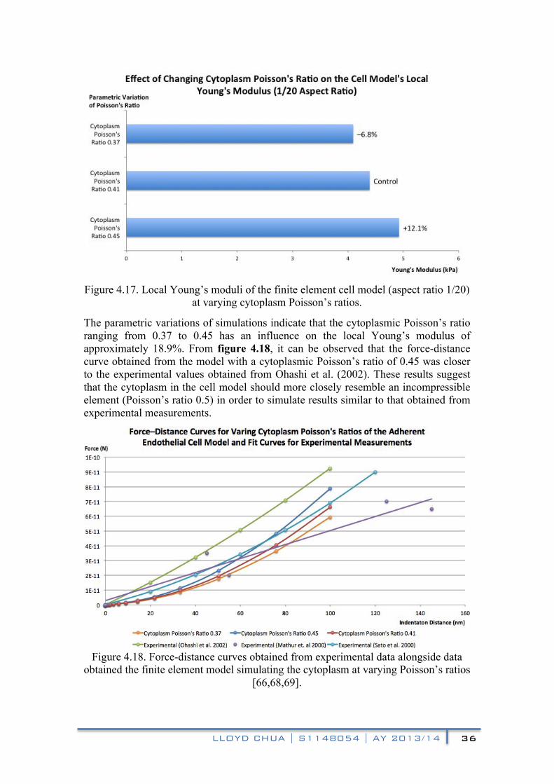
The parametric variations of simulations indicate that the cytoplasmic Poisson’s ratio ranging from 0.37 to 0.45 has an influence on the local Young’s modulus of approximately 18.9%. From figure 4.18, it can be observed that the force-distance curve obtained from the model with a cytoplasmic Poisson’s ratio of 0.45 was closer to the experimental values obtained from Ohashi et al. (2002). These results suggest that the cytoplasm in the cell model should more closely resemble an incompressible element (Poisson’s ratio 0.5) in order to simulate results similar to that obtained from experimental measurements.

Figure 4.18. Force-distance curves obtained from experimental data alongside data

obtained the finite element model simulating the cytoplasm at varying Poisson’s ratios [66,68,69].

LLOYD CHUA | S1148054 | AY 2013/14 37

4.2.5 Simulating Primary and Secondary Cancer Cells

The project’s impetus towards implementing a finite element model of a living cell was to ultimately use the validated model to simulate AFM experiments of primary and secondary cancer cells (A. Downes, unpublished). As there is a scarcity of published literature on the sub-cellular properties of cancer cells, a parametric analysis was originally intended in order to determine the sub-cellular properties of the cancer cells which would produce the same measurements as those obtained from AFM experiments. However, due to unforeseen circumstances, the experimental AFM measurements (which are a component of another BEng project) were unavailable for comparison. As such, the parametric variations originally intended for this section of simulations and analysis was omitted.

Figure 4.19. SRS microscopy images of primary–SW480 cancer cell (top) and

secondary–SW620 cancer cell lines. Each image is scaled to 200 !", with the focal distance (from substrate) shown in the top left. The cell and nucleus dimensions of the primary and secondary cells were determined from the 5 !" and 4 !" focal distances

respectively (left), while the approximate cell heights were determined from the 11 !" and 9 !" focal distances respectively (right). Circles indicate the chosen primary (red) and secondary (blue) cells used for the simulations (A. Downes, unpublished).

LLOYD CHUA | S1148054 | AY 2013/14 38

The primary and secondary cancer cells were modelled using stimulated Raman scattering (SRS) microscopy images. The cell and nucleus sizes were determined using pixel measurements of the images. The aspect ratios of the cells were determined by changing the focal lengths to determine the approximate height of the respective cells. Figure 4.19 depicts the SRS microscopy images as well as the cells that were simulated. Figure 4.20 shows the finite element models of the cells modelled after the visually determined dimensions. It can be observed that the nucleus of the primary cancer cell occupies a larger region of the cell than the secondary cell.

Figure 4.20. Finite element models of the selected primary (a) and secondary (b)

cancer cells.

The primary–SW480 and secondary–SW620 cancer cells were modelled with substrate contact lengths of 24.3 !" and 14.1 !", cell heights of 11 !" and 9 !", and nucleus lengths of 15.7 !" and 7.85 !" respectively. Figures 4.21, 4.22, and 4.23 show the force-distance, stiffness, and Young’s modulus data obtained from the two models.

Figure 4.21. Force-distance curves obtained from the simulated primary–SW480

(green) and secondary–SW620 (red) cancer cell models.

Cell stiffness is an alternative albeit more uncommon unit of measurement to define the mechanical properties of a cell. While the Young’s modulus is a property of the constituent material that does not depend on the quantity of the material (intensive),

(a) (b)

LLOYD CHUA | S1148054 | AY 2013/14 39

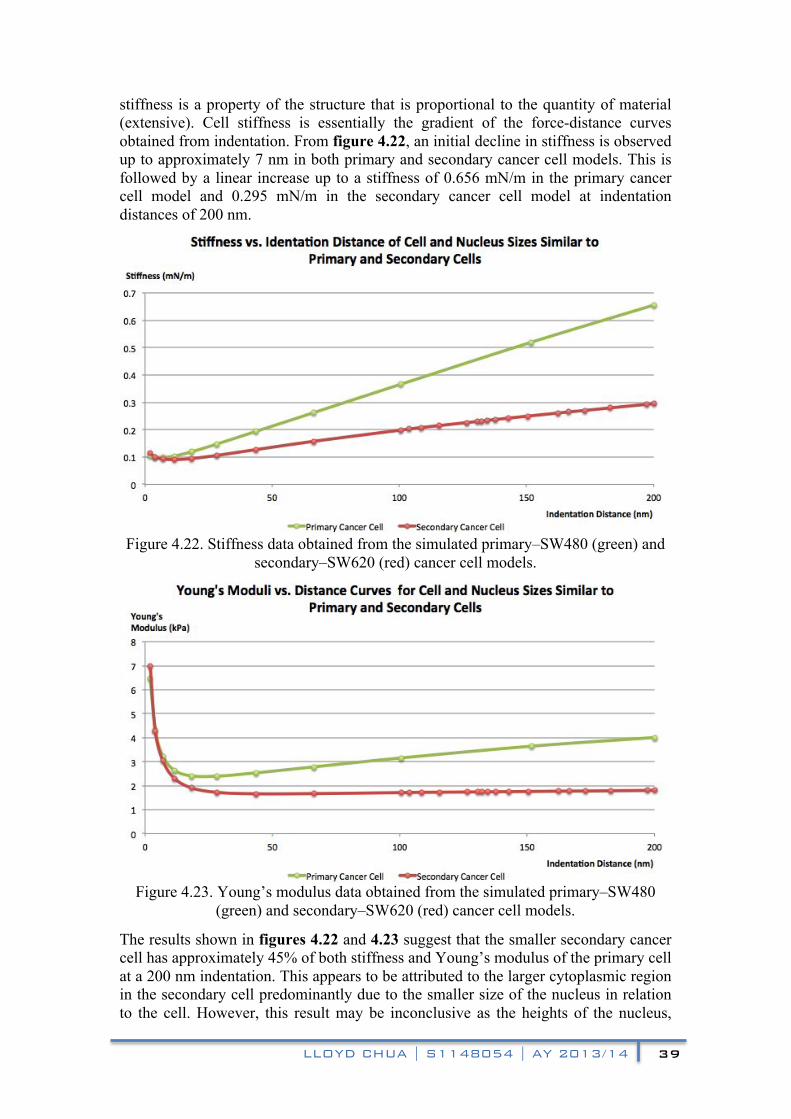
stiffness is a property of the structure that is proportional to the quantity of material (extensive). Cell stiffness is essentially the gradient of the force-distance curves obtained from indentation. From figure 4.22, an initial decline in stiffness is observed up to approximately 7 nm in both primary and secondary cancer cell models. This is followed by a linear increase up to a stiffness of 0.656 mN/m in the primary cancer cell model and 0.295 mN/m in the secondary cancer cell model at indentation distances of 200 nm.

Figure 4.22. Stiffness data obtained from the simulated primary–SW480 (green) and

secondary–SW620 (red) cancer cell models.

Figure 4.23. Young’s modulus data obtained from the simulated primary–SW480 (green) and secondary–SW620 (red) cancer cell models.

The results shown in figures 4.22 and 4.23 suggest that the smaller secondary cancer cell has approximately 45% of both stiffness and Young’s modulus of the primary cell at a 200 nm indentation. This appears to be attributed to the larger cytoplasmic region in the secondary cell predominantly due to the smaller size of the nucleus in relation to the cell. However, this result may be inconclusive as the heights of the nucleus,

LLOYD CHUA | S1148054 | AY 2013/14 40

which influences the size of the cytoplasmic region beneath the indentation is unknown and estimated in the model.

Another observation is that the larger cytoplasmic region in the secondary cancer cell allows the Young’s modulus to stabilise (1.8 kPa) at a relatively smaller indentation (from 30 nm onwards), while the Young’s modulus of the primary cancer cell continues to increase (up to 4 kPa) at a decayed rate up to the maximum indentation (200 nm). This indicates that the interaction between the sub-cellular components influencing the measured Young’s modulus become more complex as the nucleus approaches the plasma membrane in a highly spread cell. Therefore, the indentation distance when used to determine Young’s moduli in AFM measurements become increasingly significant as more sub-cellular components are involved.

4.2.6 Limitations

While the current finite element model was able to provide reasonable approximations of cell elasticity in comparison with experimental measurements, it is important to recognise the model’s relative simplicity in contrast with a real living cell. As the model attempts to replicate a cell’s complex constituents using simple geometric elements and structures, there are limitations to the model’s simulated results.

The contributions of cytoskeletal framework represented by the tensegrity network were found to be fairly limited in the model. The influence of the microtubule-struts and microfilament-cables were found to be excessively concentrated at the vertices that connect the membrane and the 6-strut 24-cable icosahedron tensegrity network. Any increase in the number of microfilament/microtubule filaments only served to increase the cross-sectional area of the struts and cables, further concentrating the cytoskeleton’s mechanical contributions to the vertices. Therefore, it was concluded that the icosahedron tensegrity finite element model, similar to the model used in McGarry and Prendergast (2004), was inadequate to evaluate the contributions of the microtubule and microfilaments for small local AFM-like indentations.

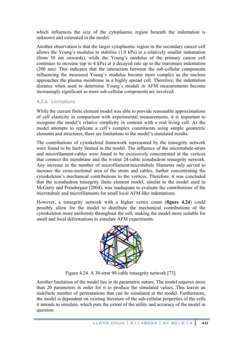
However, a tensegrity network with a higher vertex count (figure 4.24) could possibly allow for the model to distribute the mechanical contributions of the cytoskeleton more uniformly throughout the cell, making the model more suitable for small and local deformations to simulate AFM experiments.

Figure 4.24. A 30-strut 90-cable tensegrity network [73].

Another limitation of the model lies in its parametric nature. The model requires more than 20 parameters in order for it to produce the simulated values. This leaves an indefinite number of permutations that can be simulated in the model. Furthermore, the model is dependent on existing literature of the sub-cellular properties of the cells it intends to simulate, which puts the extent of the utility and accuracy of the model in question.

LLOYD CHUA | S1148054 | AY 2013/14 41

5 Conclusions The finite element cell model was firstly validated against experimental measurements of endothelial cell elasticity. Modelled after cells used in experiments conducted by Ohashi et al. (2002), it was found that the model underestimated experimental force-distance values by 34%. The underestimations were attributed to three possible sources. Firstly, the deficiency of the tensegrity structure in distributing the mechanical contributions of the cytoskeletal filaments uniformly across the cell caused the measurements at the centre of the cell to be lower than expected. The dimensions of the nucleus, which was found to play a substantial role in local measurements of Young’s modulus, were not provided in the experimental data. Lastly, the cytoplasm was found to more closely resemble an incompressible fluid (Poisson’s ratio 0.5) to in order to more accurately model experimental data.

Between cell aspect ratios of 1/5 to 1/20, the parametric variations of individual sub-cellular properties yielded elasticity values ranging up to 260%, 175%, and 129% for the cytoplasm, plasma membrane, and nucleus, respectively. These results indicate that in most instances where the nucleus is not in close proximity to the indentation site, the properties of the cytoplasm have the largest influence amongst the sub-cellular components on the cell’s elasticity, followed by the plasma membrane. However, the results of the parametric study indicated that the aspect ratio of a cell had the most significant influence on the measurement of cell elasticity, accounting for variations in Young’s modulus of up to 276% between aspect ratios 1/5 and 1/20, and 331% (between aspect ratios 1 and 1/20). The cell shape was found to be the predominant influence as it governs the arrangement of sub-cellular components being deformed by an AFM indenter for the measurement of cell elasticity.

Preliminary simulations of cells similar in dimensions with primary and secondary cancer cells indicate that the smaller secondary-SW620 cancer cell had an approximately 45% the elastic modulus and stiffness of the primary-SW480 cancer cells. These results were largely attributed to approximate geometrical dimensions of the cells and nuclei obtained from SRS microscopy images.

Overall, the model proved to be reasonably successful in replicating experimental results. The parametric studies of the cells have provided a numerical basis to assist in the understanding of the sub-cellular mechanical contributions within cells as well as the measurement of cell elasticity using AFM. Future iterations of the model would perhaps improve the uniformity of the cytoskeletal contributions throughout the cell model in order to address the underestimated values, as well as to mitigate the limitations of the model. While the initial project objective of conducting a parametric study of primary and secondary cancer cells was unsatisfied due to external circumstances, the project produced a user-friendly model generating GUI that allows for simulations to be conducted post project submission. This allows for the parametric study of the primary and secondary cancer cells to be conducted whenever the experimental measurements are finalised.

LLOYD CHUA | S1148054 | AY 2013/14 42

References [1] Dike, L. E., Chen, C. S., Mrksich, M., Tien, J., Whitesides, G. M., & Ingber, D. E.

(1999). Geometric control of switching between growth, apoptosis, and differentiation during angiogenesis using micropatterned substrates. In Vitro Cellular & Developmental Biology-Animal, 35(8), 441-448.

[2] Huang, S., & Ingber, D. E. (2000). Shape-dependent control of cell growth, differentiation, and apoptosis: switching between attractors in cell regulatory networks. Experimental cell research, 261(1), 91-103.

[3] Chen, C. S., Mrksich, M., Huang, S., Whitesides, G. M., & Ingber, D. E. (1997). Geometric control of cell life and death. Science, 276(5317), 1425-1428.

[4] Katira, P., Bonnecaze, R. T., & Zaman, M. H. (2013). Modeling the mechanics of cancer: effect of changes in cellular and extra-cellular mechanical properties. Frontiers in oncology, 3.

[5] Katira, P., Zaman, M. H., & Bonnecaze, R. T. (2012). How changes in cell mechanical properties induce cancerous behavior. Physical review letters, 108(2), 028103.

[6] Swaminathan, V., Mythreye, K., O'Brien, E. T., Berchuck, A., Blobe, G. C., & Superfine, R. (2011). Mechanical stiffness grades metastatic potential in patient tumor cells and in cancer cell lines. Cancer research, 71(15), 5075-5080.

[7] Xu, W., Mezencev, R., Kim, B., Wang, L., McDonald, J., & Sulchek, T. (2012). Cell stiffness is a biomarker of the metastatic potential of ovarian cancer cells. PloS one, 7(10), e46609.

[8] Rebelo, L. M., de Sousa, J. S., Mendes Filho, J., & Radmacher, M. (2013). Comparison of the viscoelastic properties of cells from different kidney cancer phenotypes measured with atomic force microscopy. Nanotechnology, 24(5), 055102.

[9] Cross, S. E., Jin, Y. S., Rao, J., & Gimzewski, J. K. (2007). Nanomechanical analysis of cells from cancer patients. Nature nanotechnology, 2(12), 780-783.

[10] Cassimeris, L., Plopper, G., & Lingappa, V. R. (2011). Lewin's cells. Jones & Bartlett Publishers.

[11] Heuser, J. E., & Kirschner, M. (1980). Filament organization revealed in platinum replicas of freeze-dried cytoskeletons. The Journal of cell biology, 86(1), 212-234.

[12] Fey, E. G., Wan, K. M., & Penman, S. (1984). Epithelial cytoskeletal framework and nuclear matrix-intermediate filament scaffold: three-dimensional organization and protein composition. The Journal of cell biology, 98(6), 1973-1984.

[13] Human Protein Atlas. n.d. The Human Protein Atlas. [online] Available at: http://www.proteinatlas.org/dictionary/cell [Accessed: 9 Feb 2014].

LLOYD CHUA | S1148054 | AY 2013/14 43

[14] Cooper, G. M., & Hausman, R. E. (2000). The cell. Sunderland: Sinauer Associates.

[15] Brangwynne, C. P., MacKintosh, F. C., Kumar, S., Geisse, N. A., Talbot, J., Mahadevan, L., ... & Weitz, D. A. (2006). Microtubules can bear enhanced compressive loads in living cells because of lateral reinforcement. The Journal of cell biology, 173(5), 733-741.

[16] Pollard, T. D., & Cooper, J. A. (2009). Actin, a central player in cell shape and movement. Science, 326(5957), 1208-1212.

[17] Curtis, H. & Barnes, N. S. (1989). Biology. New York, N.Y.: Worth Publishers. [18] Hine, R. (1999). The facts on file dictionary of biology. New York, NY: Facts On

File. [19] Chen, A., & Moy, V. T. (2000). Cross-linking of cell surface receptors enhances

cooperativity of molecular adhesion. Biophysical Journal, 78(6), 2814-2820. [20] Kuchel, P. W. (1988). Theory and problems of biochemistry. New York:

Mcgraw-Hill. [21] Kamm, R. D., McVittie, A. K., & Bathe, M. (2000). On the role of continuum

models in mechanobiology. ASME Applied Mechanics Division-Publications-AMD, 242, 1-12.

[22] Lulevich, V., Zimmer, C. C., Hong, H. S., Jin, L. W., & Liu, G. Y. (2010). Single-cell mechanics provides a sensitive and quantitative means for probing amyloid-β peptide and neuronal cell interactions. Proceedings of the National Academy of Sciences, 107(31), 13872-13877.

[23] Osborn, M., & Weber, K. (1976). Cytoplasmic microtubules in tissue culture cells appear to grow from an organizing structure towards the plasma membrane. Proceedings of the National Academy of Sciences, 73(3), 867-871.

[24] Guilak, F., Tedrow, J. R., & Burgkart, R. (2000). Viscoelastic properties of the cell nucleus. Biochemical and biophysical research communications, 269(3), 781-786.

[25] Caille, N., Thoumine, O., Tardy, Y., & Meister, J. J. (2002). Contribution of the nucleus to the mechanical properties of endothelial cells. Journal of biomechanics, 35(2), 177-187.

[26] Ingber, D. E. (2003). Tensegrity I. Cell structure and hierarchical systems biology. Journal of Cell Science, 116(7), 1157-1173.

[27] Lipowsky, R. (n.d.). Semi-flexible polymers and filaments. [online] Retrieved from: http://www.mpikg.mpg.de/rl/3F/ [Accessed: 16 Feb 2014].

[28] Qin, Z., Buehler, M. J., & Kreplak, L. (2010). A multi-scale approach to understand the mechanobiology of intermediate filaments. Journal of biomechanics, 43(1), 15-22.

[29] Barreto, S., Clausen, C. H., Perrault, C. M., Fletcher, D. A., & Lacroix, D. (2013). A multi-structural single cell model of force-induced interactions of cytoskeletal components. Biomaterials.

LLOYD CHUA | S1148054 | AY 2013/14 44

[30] Wang, N., & Ingber, D. E. (1994). Control of cytoskeletal mechanics by extracellular matrix, cell shape, and mechanical tension. Biophysical journal, 66(6), 2181-2189.

[31] Shin, D., & Athanasiou, K. (1999). Cytoindentation for obtaining cell biomechanical properties. Journal of Orthopaedic Research, 17(6), 880-890.

[32] Slomka, N., & Gefen, A. (2010, January). Membrane Loads in a Compressed Skeletal Muscle Cell Computed Using a Cell-Specific Finite Element Model. In World Congress on Medical Physics and Biomedical Engineering, September 7-12, 2009, Munich, Germany (pp. 102-104). Springer Berlin Heidelberg.

[33] Gittes, F., Mickey, B., Nettleton, J., & Howard, J. (1993). Flexural rigidity of microtubules and actin filaments measured from thermal fluctuations in shape. The Journal of cell biology, 120(4), 923-934.

[34] Venier, P., Maggs, A. C., Carlier, M. F., & Pantaloni, D. (1994). Analysis of microtubule rigidity using hydrodynamic flow and thermal fluctuations. Journal of biological chemistry, 269(18), 13353-13360.

[35] Kis, A., Kasas, S., Babić, B., Kulik, A. J., Benoit, W., Briggs, G. A. D., ... & Forro, L. (2002). Nanomechanics of microtubules. Physical Review Letters, 89(24), 248101.

[36] Chen, T. J., Wu, C. C., & Su, F. C. (2012). Mechanical models of the cellular cytoskeletal network for the analysis of intracellular mechanical properties and force distributions: A review. Medical engineering & physics.

[37] Fuchs, E., & Cleveland, D. W. (1998). A structural scaffolding of intermediate filaments in health and disease. Science, 279(5350), 514-519.

[38] Yasuda, R., Miyata, H., & Kinosita Jr, K. (1996). Direct measurement of the torsional rigidity of single actin filaments. Journal of molecular biology, 263(2), 227-236.

[39] Lim, C. T., Zhou, E. H., & Quek, S. T. (2006). Mechanical models for living cells—a review. Journal of biomechanics, 39(2), 195-216.

[40] Yeung, A., & Evans, E. (1989). Cortical shell-liquid core model for passive flow of liquid-like spherical cells into micropipets. Biophysical journal, 56(1), 139-149.

[41] Tsai, M. A., Frank, R. S., & Waugh, R. E. (1993). Passive mechanical behavior of human neutrophils: power-law fluid. Biophysical journal, 65(5), 2078-2088.

[42] Dong, C., Sung, K. L. P., Schmid-Schönbein, G. W., Chien, S., & Skalak, R. (1988). Passive deformation analysis of human leukocytes. Journal of biomechanical engineering, 110(1), 27-36.

[43] Stamenović, D., & Coughlin, M. F. (1999). The role of prestress and architecture of the cytoskeleton and deformability of cytoskeletal filaments in mechanics of adherent cells: a quantitative analysis. Journal of Theoretical Biology, 201(1), 63-74.

[44] Sollich, P. (1998). Rheological constitutive equation for a model of soft glassy materials. Physical Review E, 58(1), 738.

LLOYD CHUA | S1148054 | AY 2013/14 45

[45] Fabry, B., Maksym, G. N., Butler, J. P., Glogauer, M., Navajas, D., & Fredberg, J. J. (2001). Scaling the microrheology of living cells. Physical review letters, 87(14), 148102.

[46] Schmid-Schönbein, G. W., Sung, K. L., Tözeren, H., Skalak, R., & Chien, S. (1981). Passive mechanical properties of human leukocytes. Biophysical Journal, 36(1), 243-256.

[47] Coughlin MF, Stamenovi´c D.(2003)A prestressed cable network model of adherent cell cytoskeleton. Biophys. J., 84: 1328–1336.

[48] Paul, R., Heil, P., Spatz, J. P., & Schwarz, U. S. (2008). Propagation of mechanical stress through the actin cytoskeleton toward focal adhesions: model and experiment. Biophysical journal, 94(4), 1470-1482.

[49] Ingber, D. E. (1997). Tensegrity: the architectural basis of cellular mechanotransduction. Annual review of physiology, 59(1), 575-599.

[50] Stamenović, D., Fredberg, J. J., Wang, N., Butler, J. P., & Ingber, D. E. (1996). A microstructural approach to cytoskeletal mechanics based on tensegrity. Journal of Theoretical Biology, 181(2), 125-136.

[51] Wang, N., Naruse, K., Stamenović, D., Fredberg, J. J., Mijailovich, S. M., Tolić-Nørrelykke, I. M., ... & Ingber, D. E. (2001). Mechanical behavior in living cells consistent with the tensegrity model. Proceedings of the National Academy of Sciences, 98(14), 7765-7770.

[52] Scarr, G. (2010). Simple geometry in complex organisms. Journal of bodywork and movement therapies, 14(4), 424-444.

[53] Ingber, D. E. (2008). Tensegrity and mechanotransduction. Journal of bodywork and movement therapies, 12(3), 198-200.

[54] Wendling, S., Oddou, C., & Isabey, D. (1999). Stiffening response of a cellular tensegrity model. Journal of theoretical biology, 196(3), 309-325.

[55] Skelton, R. E., Adhikari, R., Pinaud, J. P., Chan, W., & Helton, J. W. (2001). An introduction to the mechanics of tensegrity structures. In Decision and Control, 2001. Proceedings of the 40th IEEE Conference on (Vol. 5, pp. 4254-4259). IEEE.

[56] Canadas, P., Laurent, V. M., Oddou, C., Isabey, D., & Wendling, S. (2002). A cellular tensegrity model to analyse the structural viscoelasticity of the cytoskeleton. Journal of Theoretical Biology, 218(2), 155-173.

[57] Stamenovic, D. (2006). Models of cytoskeletal mechanics based on tensegrity. Cytoskeletal Mechanics, 103-128.

[58] Wang, N., & Stamenović, D. (2000). Contribution of intermediate filaments to cell stiffness, stiffening, and growth. American Journal of Physiology-Cell Physiology, 279(1), C188-C194.

[59] Chen, C. S., Mrksich, M., Huang, S., Whitesides, G. M., & Ingber, D. E. (1997). Geometric control of cell life and death. Science, 276(5317), 1425-1428.

[60] McGarry, J. G., & Prendergast, P. J. (2004). A three-dimensional finite element model of an adherent eukaryotic cell. Eur Cell Mater, 7, 27-33.

LLOYD CHUA | S1148054 | AY 2013/14 46

[61] Kuznetsova, T. G., Starodubtseva, M. N., Yegorenkov, N. I., Chizhik, S. A., & Zhdanov, R. I. (2007). Atomic force microscopy probing of cell elasticity. Micron, 38(8), 824-833.

[62] Sneddon, I. N. (1965). The relation between load and penetration in the axisymmetric Boussinesq problem for a punch of arbitrary profile. International Journal of Engineering Science, 3(1), 47-57.

[63] Tilney, L. G., Connelly, P. S., Vranich, K. A., Shaw, M. K., & Guild, G. M. (2000). Actin filaments and microtubules play different roles during bristle elongation in Drosophila. Journal of cell science, 113(7), 1255-1265.

[64] Slater, J. H. (2008). Engineering endothelial cell behavior via cell-surface interactions with chemically-defined nanoscale adhesion sites. ProQuest.

[65] Alieva, I. B., Zemskov, E. A., Kireev, I. I., Gorshkov, B. A., Wiseman, D. A., Black, S. M., & Verin, A. D. (2010). Microtubules growth rate alteration in human endothelial cells. BioMed Research International, 2010.

[66] Ohashi, T., Ishii, Y., Ishikawa, Y., Matsumoto, T., & Sato, M. (2002). Experimental and numerical analyses of local mechanical properties measured by atomic force microscopy for sheared endothelial cells. Bio-medical materials and engineering, 12(3), 319-327.

[67] Ngwa, W., Makrigiorgos, G. M., & Berbeco, R. I. (2011). Gold nanoparticle-aided brachytherapy with vascular dose painting: Estimation of dose enhancement to the tumor endothelial cell nucleus. Medical physics, 39(1), 392-398.

[68] Sato, M., Nagayama, K., Kataoka, N., Sasaki, M., & Hane, K. (2000). Local mechanical properties measured by atomic force microscopy for cultured bovine endothelial cells exposed to shear stress. Journal of biomechanics, 33(1), 127-135.

[69] Mathur, A. B., Truskey, G. A., & Monty Reichert, W. (2000). Atomic force and total internal reflection fluorescence microscopy for the study of force transmission in endothelial cells. Biophysical Journal, 78(4), 1725-1735.

[70] Ofek, G., Natoli, R. M., & Athanasiou, K. A. (2009). Mechanical properties of the chondrocyte cytoplasm and nucleus. Journal of biomechanics, 42(7), 873-877.

[71] Niwayama, R., Shinohara, K., & Kimura, A. (2011). Hydrodynamic property of the cytoplasm is sufficient to mediate cytoplasmic streaming in the Caenorhabiditis elegans embryo. Proceedings of the National Academy of Sciences, 108(29), 11900-11905.

[72] Natoli, R. M. (2008). Impact Loading and Functional Tissue Engineering of Articular Cartilage. ProQuest.

[73] Li, Y., Feng, X. Q., Cao, Y. P., & Gao, H. (2010). Constructing tensegrity structures from one-bar elementary cells. Proceedings of the Royal Society A: Mathematical, Physical and Engineering Science, 466(2113), 45-61.

LLOYD CHUA | S1148054 | AY 2013/14 47

Appendix A: Model Generating GUI Documentation A.1 Setup Instructions

1. Uncompress Matlab files in desired working folder. 2. Set the same folder as the working directory in Abaqus CAE, “File > Set

Work Directory”. 3. Open GUI_1.m for suspended cell or GUI_2.m for spread cell and run

script. Select “Change Folder” to set the current folder as the Matlab working directory.

Figure A.1. Prompt window for step 3.

4. Input desired simulation parameters (see section A.3) and select “Generate Model” (macro text file “abaqusmacro.py” is created in the folder).

5. In Abaqus CAE, select “File > Macro Manager > Macro1 > Run” to run the macroinstructions that generates the model according to the parameters and starts the simulation automatically (refer to section A.4 for error troubleshooting).

Figure A.2. Abaqus macro manager.

o Abaqus will first generate 5 components (nucleus, membrane, cytoplasm, cytoskeleton, indenter), create interaction properties, mesh the parts, and apply boundary conditions and indentation conditions.

Figure A.3. Abaqus status window indicating complete model generation.

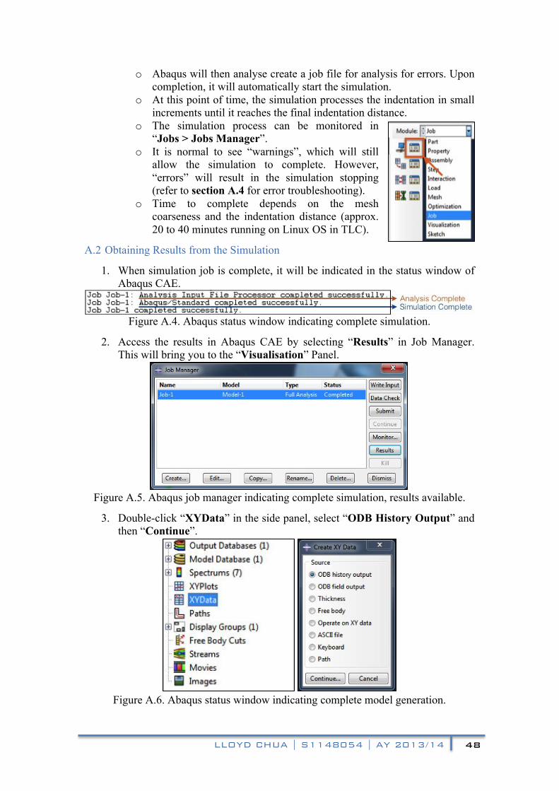
LLOYD CHUA | S1148054 | AY 2013/14 48

o Abaqus will then analyse create a job file for analysis for errors. Upon completion, it will automatically start the simulation.

o At this point of time, the simulation processes the indentation in small increments until it reaches the final indentation distance.

o The simulation process can be monitored in “Jobs > Jobs Manager”.

o It is normal to see “warnings”, which will still allow the simulation to complete. However, “errors” will result in the simulation stopping (refer to section A.4 for error troubleshooting).

o Time to complete depends on the mesh coarseness and the indentation distance (approx. 20 to 40 minutes running on Linux OS in TLC).

A.2 Obtaining Results from the Simulation

1. When simulation job is complete, it will be indicated in the status window of Abaqus CAE.

Figure A.4. Abaqus status window indicating complete simulation.

2. Access the results in Abaqus CAE by selecting “Results” in Job Manager. This will bring you to the “Visualisation” Panel.

Figure A.5. Abaqus job manager indicating complete simulation, results available.

3. Double-click “XYData” in the side panel, select “ODB History Output” and then “Continue”.

Figure A.6. Abaqus status window indicating complete model generation.

LLOYD CHUA | S1148054 | AY 2013/14 49

4. The simulation produces 2 main outputs: (1) Reaction forces at the indenter “Reaction Force: RF2 PI: Part 5-1 Node 1 in NSET AFM”, (2) Indentation Distance “Spatial Displacement: U2 PI: PART 2-1 Node 2 in NSET Indentation Point”.

Figure A.7. Abaqus history outputs window.

5. Select “Save As…” and click “OK” for each output to generate “XYData-1” and “XYData-2”.

Figure A.8. Abaqus output saving window.

LLOYD CHUA | S1148054 | AY 2013/14 50

6. Right clicking “XYData-1” and “XYData-2” individually and selecting “Edit” produces two data tables containing the reaction forces (left) and indentation distances (right) at each increment. The units of the reaction forces and indentation distances are Newtons and nanometres respectively. The X-column of each table shows the fraction of each increment from zero (0 nm indentation) to one (final indentation distance), while the Y-column shows the data at each increment.

Figure A.9. Abaqus status window indicating complete model generation.

7. Transfer the data the respective columns in the excel sheet provided “Data Sheet.xlsx” to obtain elastic modulus and stiffness data.

Figure A.10. Excel data sheet requires output data from Abaqus.

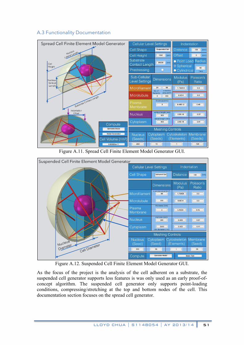
LLOYD CHUA | S1148054 | AY 2013/14 51

A.3 Functionality Documentation

Figure A.11. Spread Cell Finite Element Model Generator GUI.

Figure A.12. Suspended Cell Finite Element Model Generator GUI.

As the focus of the project is the analysis of the cell adherent on a substrate, the suspended cell generator supports less features is was only used as an early proof-of-concept algorithm. The suspended cell generator only supports point-loading conditions, compressing/stretching at the top and bottom nodes of the cell. This documentation section focuses on the spread cell generator.

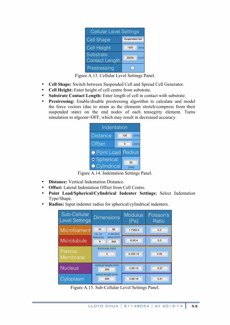
LLOYD CHUA | S1148054 | AY 2013/14 52

Figure A.13. Cellular Level Settings Panel.

• Cell Shape: Switch between Suspended Cell and Spread Cell Generator. • Cell Height: Enter height of cell centre from substrate. • Substrate Contact Length: Enter length of cell in contact with substrate. • Prestressing: Enable/disable prestressing algorithm to calculate and model

the force vectors (due to strain as the elements stretch/compress from their suspended state) on the end nodes of each tensegrity element. Turns simulation to nlgeom=OFF, which may result in decreased accuracy.

Figure A.14. Indentation Settings Panel.

• Distance: Vertical Indentation Distance. • Offset: Lateral Indentation Offset from Cell Centre. • Point Load/Spherical/Cylindrical Indenter Settings: Select Indentation

Type/Shape. • Radius: Input indenter radius for spherical/cylindrical indenters.

Figure A.15. Sub-Cellular Level Settings Panel.

LLOYD CHUA | S1148054 | AY 2013/14 53

• Dimensions: input values for dimensions for sub-cellular components. o No. of filaments (top/bottom): input number of microfilaments in a

cell (top), input number of microtubules in a cell (bottom). o X-section area (top/bottom): input average cross-sectional area of

each microfilament (top) and microtubule (bottom) in a cell. o Thickness: Input plasma membrane thickness. o Vertical Height: Input vertical height of nucleus. o Lateral Length: Input lateral length of nucleus.

• Modulus: Input Young’s modulus of each sub-cellular component. • Poisson’s Ratio: Input Poisson’s Ratio of each sub-cellular component.

Figure A.16. Meshing Controls Panel.

It is recommended to maximise number of seeds for the software license (20,000 total nodes for academic license).

• Nucleus (Seeds): Input Global Size of Nucleus (smaller = finer mesh). • Cytoplasm (Seeds): Input number of seeds on Cytoplasm vertical edge. Seeds

are biased towards the cell centre (figure A.17). • Cytoskeleton (Elements): Input number of elements per tensegrity element

(recommended: 1) (figure A.17). • Membrane Seeds: Input number of seeds on the cells top edges (figure A.17).

Figure A.17. Seeding configurations. Membrane Seeds (orange) determines the

number of seeds at the outer edge, Cytoplasm Seeds (red) determines the number of seeds at the vertical edge, Nucleus Seeds (blue) determines the number of seeds at the nucleus edge, Cytoskeleton Elements (green) determines the number of elements that

make up a single strut/cable.

LLOYD CHUA | S1148054 | AY 2013/14 54

Figure A.18. Computation Panel.

• Generate Model: Run Algorithm to print Macro to generate model in Abaqus.

• Status Box: Reports Model Generated when complete. • Cell Volume: Presents calculated cell volume for the dimensions input. To be

used as reference if cell volume is desired to be kept constant.

A.4 Error Troubleshooting

As there is a large permutation of possible settings, it was unable to exhaustively test the model generator GUI. The GUI functions as designed using the default input parameters. Any large deviation from the default parameters may cause the simulation to fail. Any minor alteration of the GUI script is likely to cause the macroinstruction to be unusable by Abaqus. As such, it is recommended that a user have good understanding of the scripting process before alterations are made. Minor alterations to the model may be made within Abaqus CAE without much risk of a failed simulation. The following is a list of factors that may contribute to the failure of simulation within Abaqus:

• Excessive number of seeds in meshing may cause the model to generate a total number of nodes that exceeds the academic license (20,000 nodes). Reduce the number of seeds and regenerate model to resolve.

• Large indentation distances may cause the simulation to run for excessively long periods. This is due to the software reducing the increment size as the problem becomes more complex. At large indentations, a large number of elements are being calculated. As such, the simulation may fail before it reaches the final indentation distance. However, all data up to the failure point can still be used and accessed. Reduce the indentation distance to resolve.

• Simulation may fail if the microfilament/microtubule count is increased and a large indentation is made directly on a tensegrity vertex. This is due to the relatively high modulus of the tensegrity structure, and a large deformation causes an unexpectedly large deformation to the structure. Adjust the indentation offset to ensure that indentation is not too close to a tensegrity vertex to resolve.

• Model generation failures may result if the input dimensions generate impossible geometries (i.e. nucleus vertical height larger than cell height). The algorithm produces a macro that instructs Abaqus to generate the model by following set steps. Check input dimensions or start by making small changes to default parameters to resolve. Alternatively, checking the point at which the Abaqus model generation fails may help to narrow down the cause of the error.