Automotive OLED Life Test and Prediction Paul Weindorf, Daniel Andres, Jeff Hatfield

Visteon Corporation, Van Buren Township, Michigan, USAFutaba Corporation, Plymouth, Michigan USA

pweindor@visteon.com, dandres@visteon.com, jhatfield@futaba.com

Abstract:A 10,000 hour operational life test at 25°C, 60°C, and 85°C was performed on Futaba automotive OLED displays. Luminance degradation results are reported together with an automotive life cycle prediction for aging performance.

Keywords/Acronyms: OLED – Organic Light Emitting DiodeVFD – Vacuum Fluorescent DisplayTFT – Thin Film TransistorLCD – Liquid Crystal DisplaySTN – Super Twisted NematicLife TestAging

1. IntroductionLight valve based display technologies, such as utilized in TFT displays, depend on a general light source that decays over time. Light valve based displays do not suffer from differential aging where portions of the display used more frequently will emit less light than other portions used less frequently. Although OLED displays have many benefits, the emissive nature of the technology results in luminance aging that is accelerated substantially at elevated temperatures commonly associated with automotive environments. Understanding and predicting the amount of luminance degradation is important to determine if OLED displays may be successfully utilized in automotive applications. Only Futaba OLED displays were life tested since Futaba is the only remaining supplier of passive matrix automotive OLEDs. The adjoining automotive luminance prediction is an extension of methods previously reported [1]. In spite of the differential aging disadvantage, the motivation for evaluating OLED displays is for the advantages afforded when compared to LCD (especially STN) technologies:

Higher contrast ratios Superior color and contrast viewing angle performance No black background luminance “bleed” Better reflectance performance Substantially better power performance

The power performance advantage is primarily due to emissive nature of the technology whereby only the pixels that need to be utilized consume power as compared to LCD technologies where the backlight must essentially “light up” all the pixels all the time thereby absorbing lighting energy not seen by the user. An example of the power consumption characteristic as a function of the pixel usage is depicted in Figure 1-1. As the automotive industry is driven to improve fuel economies and extend the range of electric vehicles, power conservation is becoming a more important parameter.

Figure 1-1: 2” OLED Power Consumption versus Usage % Figure 1-2 depicts examples of different lighting usage rates.

Figure 1-2: Lighting Usage Rate Examples

2. OLED Life Test Description The OLED life test consisted of operating three Futaba OLED displays as shown in Figure 2-1. The Futaba EL427 displays have the following key attributes:

1. Duty -1/642. Color - White3. Luminance – 300 cd/m2 with circular polarizer

1

Figure 2-1: Futaba OLED DisplayPrior to starting the test, the OLEDs were characterized using a PR705 spectroradiometer with the results as shown in Table 2-1. The display pattern measured and used during the test consisted of four different gray shade areas (zones A, B, C, D) as shown in Figure 2-2 which also shows the measurement locations for Table 2-1. The four drive levels are:L4 – highest drive (white) L3 – approximately ½ of L4 driveL2 – approximately ½ of L3 driveL1 – No drive (black) In addition, “all white” and “all black” display measurements were made at location “E” in the center of the display where the entire screen was driven to the L4 (all white) and L1 (all black) drive levels. The PR705 spot size diameter subtended 8.5 display pixels.The display luminance for each of the four areas was measured in real time by utilizing four Osram BPW 34 S clear light sensors with a radiant sensitive area of 7mm2 as shown in Figure 2-3. The clear sensor was utilized to increase the signal to noise level versus the use of a photopic filter type sensor since all the measurements are relative in nature.

OLED Measurement cd/m2 x y

ID Location(drive level)

#1 A (L3 drive) 130.4 0.3027 0.3113

#1 B (L2 drive) 56.91 0.3014 0.3107

#1 C (L1 drive) 1.081 0.3142 0.3072

#1 D (L4 drive) 275.7 0.3022 0.3090

#1 E (all white L4) 269.3 0.2990 0.3070

#1 E (all black L1) 0.002285 0.3931? 0.3111?

#2 A (L3 drive) 132.4 0.3051 0.3134

#2 B (L2 drive) 57.84 0.3039 0.3129

#2 C (L1 drive) 1.103 0.3151 0.3086

#2 D (L4 drive) 284.2 0.3003 0.3103

#2 E (all white L4) 281.0 0.3029 0.3147

#2 E (all black L1) 0.003906 0.3509? 0.3045?

#3 A (L3 drive) 133.2 0.3055 0.3120

#3 B (L2 drive) 58.77 0.3038 0.3123

#3 C (L1 drive) 1.115 0.3160 0.3083

#3 D (L4 drive) 285.2 0.3016 0.3083

#3 E (all white L4) 279.5 0.3002 0.3085

#3 E (all black L1) 0.003346 0.3412 0.3001

Table 2-1: Futaba Display Measurements Prior to Life Test

A B

CD

E

Figure 2-2: Futaba OLED Initial PR 705 Measurement Locations

2

Figure 2-3: Osram Light Sensor [2]The photo sensors were mounted to a PWB with a light blocking frame around each gray shade area as shown in Figure 2-4.

Figure 2-4: Light Sensor Frame AssemblyFigure 2-5 shows the trans-impedance amplifier circuit used to convert the light sensor current into a voltage that is subsequently sampled by the microprocessor A/D converter. This circuit configuration was chosen to minimize dark current temperature errors since the voltage across the detector is controlled to zero volts.

Figure 2-5: Light Sensor Current to Voltage Converter (Light Sensor and Amplifier)

A real time data collection approach was selected instead of

measuring through the chamber window or periodically taking the units out of the chamber and measuring them. This real time data collection approach: Reduces measurement errors associated with measuring

exactly the same point through a chamber window. Allows for a continuum of data not possible with periodically

taking the units out of the chamber for measurements. This continuum of data is particularly important for obtaining the aging slope characteristics for the prediction model.

As shown in Figure 2-6, the four light sensor analog signals from the 4 light sensor amplifiers together with the precision voltage reference are input to five 12 bit analog to digital converter channels of the PIC processor.  These five signals are read at a rate of 25 times per second and averaged.  These values are packaged into one UART message which is sent to the PC through the FT4232 UART to USB converter. 

Figure 2-6: System Block DiagramThe Visual Basic PC program collects the UART messages from the 3 light sensor/PIC assemblies, then processes and stores the data in the appropriate locations.  The data is converted to decimal and stored on the PC hard drive in a .csv format for importing into Microsoft Excel for processing and saved at a user defined interval.  The program also has an elapsed time timer, with backup in case of program or power interruption.

The three OLED displays were operated at three different temperatures:

3

1. Room Temperature (no chamber)2. 60°C Chamber Temperature3. 85°C Chamber Temperature

The test was run continuously for 10,000 hours from March of 2012 to May of 2013 and the luminance data from the light sensors was accumulated at a rate of once per minute for the first 1.3 hours and subsequently at a rate of once every ten minutes for the remainder of the test.

3. OLED Life Test ResultsThe raw data for the OLED life test is shown in Figure 3-1.

0

100

200

300

400

500

600

700

800

900

1000

0 5000 10000

Ligh

t Sen

sor A

/D C

ount

s

Hours

Room Temp:1/2Vref

Room Temp:LS4

Room Temp:LS3

Room Temp:LS2

Room Temp:LS1

60C:1/2 Vref

60C:LS4

60C:LS3

60C:LS2

60C:LS1

85C:1/2 Vref

85C:LS4

85C:LS3

85C:LS2

85C:LS1

Figure 3-1: Raw Life Test DataThe 1/2Vref values are references to ensure that the A/D converter values are working correctly. Note that the “bump” in the 85°C data is due to the chamber light being inadvertently turned on. Other than a couple of very short glitches, the data is remarkably stable and consistent. Several notable observations are immediately apparent: At the highest luminance level the luminance decay rate

increases as the operational temperature is increased. As the luminance is lowered, the luminance decay rate is less

and therefore under night time automotive operational luminance levels the luminance consumption rate is significantly reduced as will become apparent in the

forthcoming model. The curves are approximately exponential in nature

indicating a robust design with no catastrophic mechanism that changes the shape of the curve as seen on OLEDs in the 2005 timeframe [1].

Figure 3-2 shows great correlation between the Futaba test data (black rhomboids) and the Visteon data (blue circles) which adds credibility to the results of both companies.

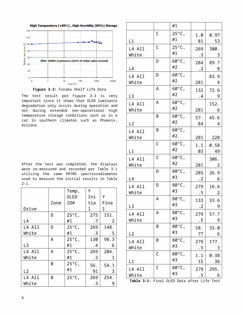
Figure 3-2: Visteon versus Futaba CorrelationThe observation that the luminance decay decreases as the luminance level is reduced is consistent with Futaba shelf life testing as shown in Figure 3-3.

Figure 3-3: Futaba Shelf Life DataThe test result per Figure 3-3 is very important since it shows that OLED luminance degradation only occurs during operation and not during extended non-operational high temperature storage conditions such as in a car in southern climates such as Phoenix, Arizona.

After the test was completed, the displays were re-measured and recorded per Table 3-1 utilzing the same PR705 spectroradiometer used to measure the initial results in Table 2-1.

Drive Temp, OLED ID#

Y Initial

YFinal

4

ZoneL4 D 25°C, #1 275.7 151.2L4 All White D 25°C, #1 269.3 148.5L3 A 25°C, #1 130.4 98.36L4 All White A 25°C, #1 269.3 204.1

L2 B 25°C, #1 56.91 54.13

L4 All White B 25°C, #1 269.3 254.9

L1 C 25°C, #1 1.081 0.9753

L4 All White C 25°C, #1 269.3 300.3

L4 D 60°C, #2 284.2 89.78

L4 All White D 60°C, #2 281 83.94

L3 A 60°C, #2 132.4 72.69

L4 All White A 60°C, #2 281 152.6

L2 B 60°C, #2 57.84 45.64

L4 All White B 60°C, #2 281 228

L1 C 60°C, #2 1.103 0.5849

L4 All White C 60°C, #2 281 306.2

L4 D 80°C, #3 285.2 26.96

L4 All White D 80°C, #3 279.5 16.62

L3 A 80°C, #3 133.2 33.69

L4 All White A 80°C, #3 279.5 57.79

L2 B 80°C, #3 58.77 33.06

L4 All White B 80°C, #3 279.5 177.3

L1 C 80°C, #3 1.115 0.3836

L4 All White C 80°C, #3 279.5 295.6Table 3-1: Final OLED Data after Life Test

Figure 3-4 shows a comparison between the initial and final luminance measurements per Tables 2-1 and 3-1. As further explanation, after the life test each of the areas were measured both with the testing drive level (e.g. L1, L2, L3, L4) and at full drive (White). Observation of the 85°C L1 (black drive) White data shows no degradation in luminance after 10,000 hours of operation which demonstrates that at low drive levels there is little or no luminance degradation.

0

50

100

150

200

250

300

350

L4

(2

5°C)

L4 W

hite

(25°

C)L3

(25°

C)L3

Whi

te (2

5°C)

L2

(2

5°C)

L2 W

hite

(25°

C)L1

(25°

C)L1

Whi

te (2

5°C)

L4

(6

0°C)

L4 W

hite

(60°

C)L3

(60°

C)L3

Whi

te (6

0°C)

L2

(6

0°C)

L2 W

hite

(60°

C)L1

(60°

C)L1

Whi

te (6

0°C)

L4

(8

5°C)

L4 W

hite

(85°

C)L3

(85°

C)L3

Whi

te (8

5°C)

L2

(8

5°C)

L2 W

hite

(85°

C)L1

(85°

C)L1

Whi

te (8

5°C)

Lum

inan

ce (c

d/m

^2)

Y Initial

Y Final

Figure 3-4: Luminance Data ComparisonFigure 3-5 shows the correlation between that light sensor system and the calibrated PR705 measurement equipment, confirming that the light sensor system did good job at dynamically measuring the OLED luminance degradation.

-100-90-80-70-60-50-40-30-20-10

0

L425°C

L325°C

L225°C

L460°C

L360°C

L260°C

L485°C

L385°C

L285°C

% D

ecre

ase

LS % Decrease

705 % Decrease

Figure 3-5: Light Sensor to PR705 Correlation

5

Initial and final color data is in shown in Table 3-2.

Drive (Zone,Temp,ID#)

x Initial

y Initial

x Final

y Final

L4 (D,25°C,#1) 0.3022 0.309 0.3313 0.3255L4 All White(D,25°C,#1) 0.299 0.307 0.3287 0.3237L3 (A,25°C,#1) 0.3027 0.3113 0.318 0.3197L4 All White (A,25°C,#1) 0.299 0.307 0.3141 0.3173L2 (B,25°C,#1) 0.3014 0.3107 0.3102 0.3159L4 All White(B,25°C,#1) 0.299 0.307 0.3115 0.3146L1 (C,25°C,#1) 0.3142 0.3072 0.2934 0.2935L4 All White(C,25°C,#1) 0.299 0.307 0.3052 0.3119L4 (D,60°C,#2) 0.3003 0.3103 0.3681 0.3439L4 All White(D,60°C,#2) 0.3029 0.3147 0.3648 0.3419L3 (A,60°C,#2) 0.3051 0.3134 0.3444 0.3316L4 All White(A,60°C,#2) 0.3029 0.3147 0.3436 0.3307L2 (B,60°C,#2) 0.3039 0.3129 0.3262 0.3236L4 All White(B,60°C,#2) 0.3029 0.3147 0.3282 0.3255L1 (C,60°C,#2) 0.3151 0.3086 0.3088 0.3029L4 All White(C,60°C,#2) 0.3029 0.3147 0.3138 0.3174L4 (D,85°C,#3) 0.3016 0.3083 0.4548 0.3846L4 All White(D,85°C,#3) 0.3002 0.3085 0.4469 0.3792L3 (A,85°C,#3) 0.3055 0.312 0.3945 0.3531L4 All White(A,85°C,#3) 0.3002 0.3085 0.3924 0.352L2 (B,85°C,#3) 0.3038 0.3123 0.3487 0.3324L4 All White(B,85°C,#3) 0.3002 0.3085 0.3491 0.3319L1 (C,85°C,#3) 0.316 0.3083 0.406 0.3465L4 All White(C,85°C,#3) 0.3002 0.3085 0.329 0.3239

Table 3-2: Initial to Final Color ComparisonFigure 3-6 shows that the color changes dramatically for the high drive levels at high temperature operation.

0.20.220.240.260.28

0.30.320.340.360.38

0.4

0.2 0.3 0.4 0.5

y

x

y Initial

y Final

Figure 3-6: Color Shift

4. Automotive Life PredictionThe life prediction method utilized is the same as used in Reference [1]. The idea behind the modeling technique is to develop a model for how the initial luminance degradation slope changes as a function of temperature. To make the mathematics manageable, and because the amount of degradation over the life of the vehicle is on the order of 10% reduction, the -10% points are first determined so that a suitable heuristic equation may be developed that describes how the -10% hours changes as a function of temperature. The -10% points are shown in Table 4-1 where the minus 10% is determined from the highest luminance after the start of the test.

Temperature HighestCount

-10%Count

-10%Hours

Room 850 765 1351

+60°C 839 755 666

+85°C 838 754 324

Table 4-1: -10% HoursThe next step is to develop a math model to calculate the -10% hours as a function of temperature. There are many possibilities, but one method is to use a slope intercept Equation 4-1.

Eq 4-1

If a value of -3 is selected for the exponent “P”, an approximately linear relationship is established between the “-10% hours” and the variable “°K-3” as shown in Figure 4-1. Table 4-2 shows the values used for the graph in Figure 4-1.

°C °K °K-3 -10% hours25 298 3.78E-08 135160 333 2.71E-08 66685 358 2.18E-08 324

Table 4-2: Selection of the Exponent “P”

6

0200400600800

1000120014001600

0 1E-08 2E-08 3E-08 4E-08

-10%

Hou

rs

1/°K^P

-10% hours

-10% hours

Figure 4-1: Selection of the Exponent “P”The slope and intercept may then be calculated per Equations 4-2 and 4-3.

Eq

4-2

Eq 4-3Substituting the calculated slope and intercept values from Equations 4-2 and 4-3 into Equation 4-1 yields Equation 4-4.

Eq 4-4A plot of Equation 4-4 with respect to the data confirms that Equation 4-4 “fits” the data as shown in Figure 4-2.

0

200

400

600

800

1000

1200

1400

1600

0 20 40 60 80 100

-10%

Hou

rs

Temperature

-10% Hours Formula-10% Hours Data

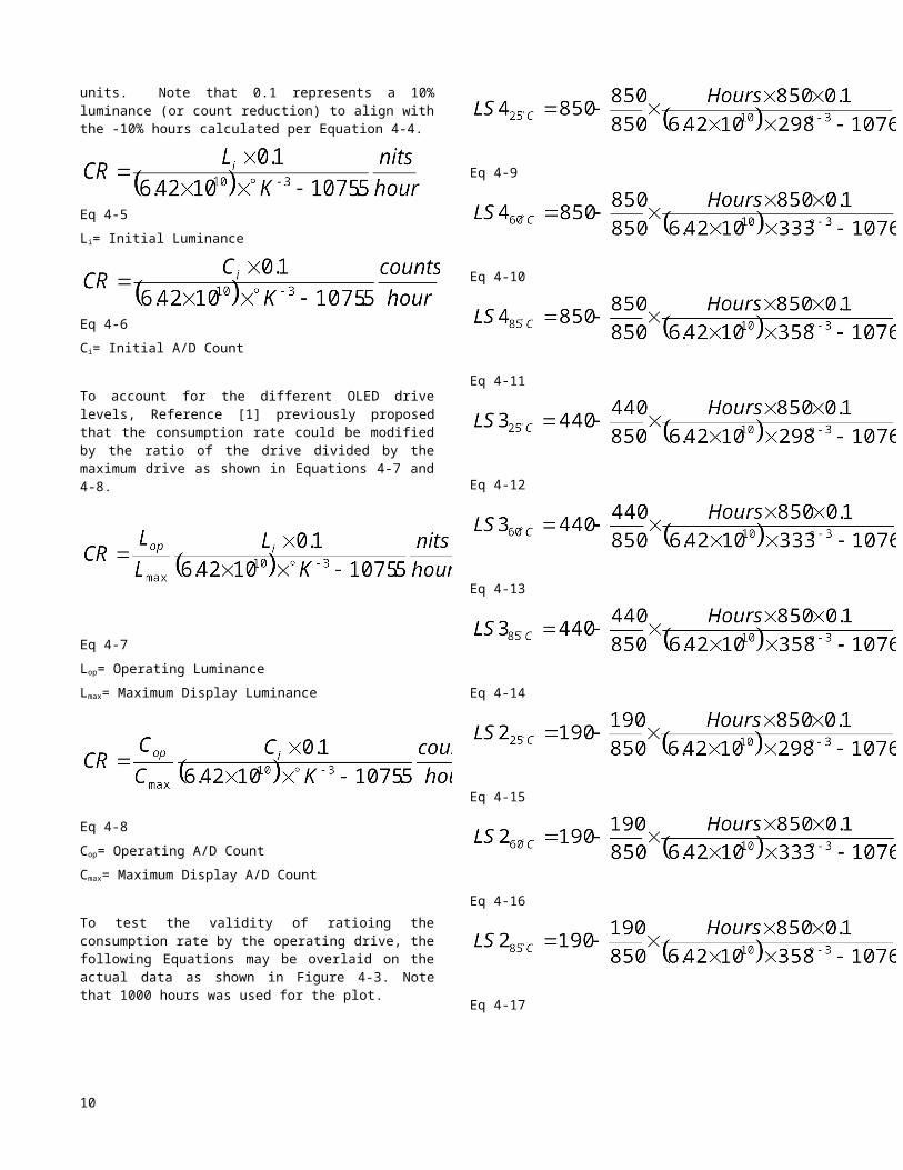
Figure 4-2: -10% Hours Curve FitUsing Equation 4-4, the consumption rate formula may be developed per Equation 4-5 or Equation 4-6 depending on whether nits/hour or A/D counts/hour are desired for the units. Note that 0.1 represents a 10% luminance (or count reduction) to align with the -10% hours calculated per Equation 4-4.

Eq 4-

5Li= Initial Luminance

Eq

4-6Ci= Initial A/D Count

To account for the different OLED drive levels, Reference [1] previously proposed that the consumption rate could be modified by the ratio of the drive divided by the maximum drive as shown in Equations 4-7 and 4-8.

Eq 4-7Lop= Operating LuminanceLmax= Maximum Display Luminance

Eq 4-8Cop= Operating A/D CountCmax= Maximum Display A/D Count

To test the validity of ratioing the consumption rate by the operating drive, the following Equations may be overlaid on the actual data as shown in Figure 4-3. Note that 1000 hours was used for the plot.

Eq 4-9

Eq 4-10

Eq 4-11

Eq 4-12

Eq 4-13

7

Eq 4-14

Eq 4-15

Eq 4-16

Eq 4-17

0

100

200

300

400

500

600

700

800

900

1000

0 2000 4000 6000 8000 10000

Ligh

t Sen

sor A

/D C

ount

s

Hours

Room Temp:LS4

Room Temp:LS3

Room Temp:LS2

60C:LS4

60C:LS3

60C:LS2

85C:LS4

85C:LS3

85C:LS2

LS4 25C Predict

LS4 60C Predict

LS4 85C Predict

LS3 25C Predict

LS3 60C Predict

LS3 85C Predict

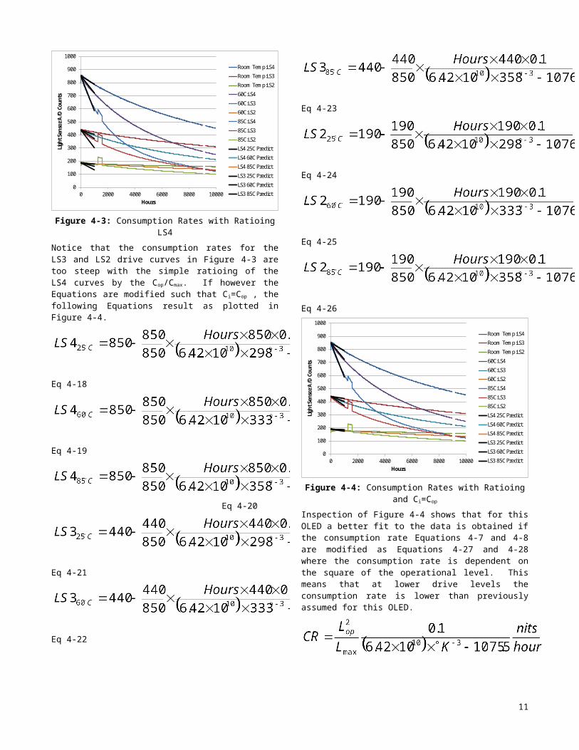
Figure 4-3: Consumption Rates with Ratioing LS4Notice that the consumption rates for the LS3 and LS2 drive curves in Figure 4-3 are too steep with the simple ratioing of the LS4 curves by the Cop/Cmax. If however the Equations are modified such that Ci=Cop , the following Equations result as plotted in Figure 4-4.

Eq 4-18

Eq 4-19

Eq 4-20

Eq 4-21

Eq 4-22

Eq 4-23

Eq 4-24

Eq 4-25

Eq 4-26

0

100

200

300

400

500

600

700

800

900

1000

0 2000 4000 6000 8000 10000

Ligh

t Sen

sor A

/D C

ount

s

Hours

Room Temp:LS4

Room Temp:LS3

Room Temp:LS2

60C:LS4

60C:LS3

60C:LS2

85C:LS4

85C:LS3

85C:LS2

LS4 25C Predict

LS4 60C Predict

LS4 85C Predict

LS3 25C Predict

LS3 60C Predict

LS3 85C Predict

Figure 4-4: Consumption Rates with Ratioing and Ci=Cop Inspection of Figure 4-4 shows that for this OLED a better fit to the data is obtained if the consumption rate Equations 4-7 and 4-8 are modified as Equations 4-27 and 4-28 where the consumption rate is dependent on the square of the operational level. This means that at lower drive levels the consumption rate is lower than previously assumed for this OLED.

Eq 4-27

Eq 4-28Equations 4-27 and 4-28 only describe the consumption rate at any one temperature (Kelvin). Next, an exponential decay temperature function may be substituted for the temperature variable to describe how the ambient temperature in the vehicle decreases from an 85°C hot start and a 20 minute time constant

8

down to 45°C yielding Equations 4-29 and 4-30. This situation may describe a hot start from a display under a solar load situation in a location like Phoenix, Arizona. The 20 minutes (0.15 hour time constant) may describe how long it takes for the air conditioning system to reduce the internal temperatures to a normal internal instrument cluster ambient of 45°C.

Eq 4-29

Eq 4-30The integral of the consumption rate formula as shown in Equation 4-30 provides the luminance degradation (LD) as a function of time.

Eq 4-31

However integration of the CR functions per Equations 4-29 and 4-30 are complex. Therefore the next step in the process is to determine a good exponential function curve fit to CR formulas in order to simplify the integration mathematics and to give a resultant formula which has separate steady state and hot start components. The starting point is to redefine the consumption rate formulas per Equations 4-32, 4-33 and 4-34.

Eq 4-32

Eq 4-33

Eq 4-34The simplified exponential formula has the form shown in Equation 4-35.

Eq 4-35

The constant terms may be determined per Equations 4-36 and 4-37.

Eq 4-36

Eq 4-37Therefore substituting Equations 4-36 and 4-37 into Equation 4-35 yields Equation 4-38.

Eq 4-38

Figure 4-5 shows a plot of the Equation 4-30 and a reasonable curve fit exponential Equation 4-38 with TC=0.1..

0

0.00005

0.0001

0.00015

0.0002

0.00025

0.0003

0.00035

0 0.5 1

f(t)

Hours

f(t)fs(t)

Figure 4-5: Curve Fit fS(t) versus f(t)The Luminance Degradation, LD, as a function of time may be determined per Equation 4-39.

Eq 4-39Solving the integral of Equation 4-39 is shown per Equation 4-40.

9

Eq 4-40Substituting the results from Equation 4-40 into Equation 4-39 yields Equation 4-41.

Eq 4-41K1= 1.08x10-4

K2= 2.01x10-4

TC= 0.1Similarly in terms of luminance, Equation 4-42 may be formulated.

Eq 4-42As an example, if the display is operated at maximum luminance, Cop=Cmax. Therefore Equation 4-41 becomes Equation 4-43.

Eq 4-43

The display at maximum luminance is about 850 A/D counts. Therefore Equation 4-43 becomes Equation 4-44.

Eq 4-

44The first term is the steady state term and so for 1000 hours of operation 91.8 counts of luminance degradation will occur which is consistent (less than) with the data where 132 counts of luminance degradation occurs at 60°C. A lower loss of luminance

is expected since the steady state temperature analyzed is 45°C.In terms of luminance the ratio of counts to nits is about 280/850=0.329 nits/count and would result in a loss in luminance of about 30 nits per 1000 hours of operation. This result is also consistent with Figure 4-2 which predicts a -10% reduction (28 nits) in luminance at about 950 hours. In terms of luminance the Luminance Degradation is calculated per Equation 4-45 for operation at 280 nits.

Eq 4-

45So per Equation 4-45, each hot start from +85°C consumes 0.0056 nits of luminance and each steady state hour of operation at 45°C consumes 0.0301 nits of luminance.If the luminance is decreased to a nighttime level of 40 nits the luminance degradation is per Equation 4-46.

Eq 4-46An automotive life example may be constructed assuming 10 years at 15K mi/year (150K mi total). At an average speed of 30 mi/hr, the total number of operational hours is 5000 hours with an estimated 3650 hot summer starts (2 hot start/summer day). The luminance degradation over the life of the vehicle may be estimated as shown in Table 4-3 using Equations 4-45 and 4-46.

Condition Luminance Decrease

Notes

3650 +85°C Hot Starts

20.44 nits 20.44=3650x.0056

2500 hours @ 280 nits Day Time Operation

75.46 nits 75.46=2500x0.030184

2500 hours @ 40 nits Night Time Operation

1.54 nits 1.54=2500x0.000616

Total Luminance Decrease @ End of Life

97.44 nits 34.8% decrease from the initial 280 nits

Table 4-3: OLED Automotive Example at 45°C Steady StateA luminance loss of 34.8% in the Table 4-3 example assumes that the display is always on in all the same locations which can occur in an automotive environment with no counter measures for image burn-in.If the OLED steady state temperature is lowered to 25°C in an instrument cluster with no lens where the OLED surface is exposed directly to the cabin environment, Equations 4-45 and 4-46 change to 4-47 (daytime 280 nits) and 4-48 (night time 40 nits).

Eq 4-

47

Eq 4-

48

10

Therefore under this 25°C steady state conditions, the automotive example changes to Table 4-4.

Condition Luminance Decrease

Notes

3650 +85°C Hot Starts

19.345 nits 19.345=3650x.0053

2500 hours @ 280 nits Day Time Operation

52.5 nits 52.5=2500x0.021

2500 hours @ 40 nits Night Time Operation

1.05 nits 1.05=2500x0.00042

Total Luminance Decrease @ End of Life

72.9 nits 26% decrease from the initial 280 nits

Table 4-4: OLED Automotive Example at 25°C Steady StateAs a sanity check of the model if the actual 25°C data is used, the luminance reduction is 48 nits which is in close agreement with the 52.5 nits calculated from the model and the error is due to the linearization of the slopes in the model as shown in Figure 4-4. Tables 4-3 and 4-4 represent the worst case conditions of a lot of 85°C hot starts and continuous static images on the display and therefore a residual image causes by a 26% to 34.8% decrease in luminance will probably be acceptable at the vehicle end of life. If counter measures such as automatic luminance control and/or image dithering are employed, the performance will be improved.

6. VF Display ComparisonIn the Detroit SID O5 paper [1], a comparison to VF life performance was presented. The Luminance Degradation (LD) Equation 6-1 was presented to estimate the amount of image burn-in on dot matrix VFDs which have been widely accepted for automotive applications. Equation 6-1 describes that 0.000118 nits of luminance is lost for each hot start from +85°C. In addition, a steady state consumption rate of 0.001461nits/hour is realized at a steady state operational temperature of 45°C.

Eq 6-

1Equation 6-1 needs to be normalized to an equivalent of 300 cd/m2 instead of 120 cd/m2 to properly compare the performance to the current OLEDs. Equation 6-2 shows the VF performance normalized to 300 cd/m2.

Eq 6-

2Table 6-1 shows a summary of the luminance degradation for 5000 hours of operation at a steady state temperature of +45°C ambient with 3650 hot starts from +85°C.

Condition

Luminance Decreasecd/m2 Notes

3650 +85° Hot Starts 1.08 1.08=3650x0.0002952500 Hours @ 300 nits Day Time Operation 9.13 9.13=2500x0.0036532500 Hours @ 40 nits Night Time Operation 1.22

1.22=2500x0.001461x40/300

Total Luminance Decrease @ End of Life 11.43

3.81% decrease from initial 300 nits

Figure 6-1: VFD Automotive Life ExampleTherefore the data suggests that the VFD display has less residual image burn-in than the OLEDs tested.

6. ConclusionsThe Futaba OLED displays operated successfully for 10,000 hours at 25°C, 60°C and 85°C. The luminance degradation measured during the test was used to predict the aging performance for a worst case automotive life cycle. The aging prediction indicates that the Futaba OLED display image burn in performance is worse than matrix type VF displays. However it is expected that the Futaba OLED display may be successfully utilized for automotive applications.

7. References[1] Weindorf, P., Automotive Life Prediction Method, Detroit SID 05 Digest.[2]http://catalog.osram-os.com/catalogue/catalogueSearchByProperty.do?act=search&action=start&favOid=00000002000095e6001b0023&oid=00000002000095e6001b0023

11