Automating Hardware and Software Evolution Analysis

Brian Dougherty, Jules White, Chris Thompson, and Douglas C. SchmidtDepartment of Electrical Engineering and Computer Science,

Vanderbilt University, Nashville, TN, USA{briand,jules,schmidt}@dre.vanderbilt.edu & chris.m.thompson@vanderbilt.edu

Abstract

Cost-effective software evolution is critical to many dis-tributed real-time and embedded (DRE) systems. Select-ing the lowest cost set of software components that meetDRE system resource constraints, such as total memory andavailable CPU cycles, is an NP-Hard problem. This paperprovides three contributions to R&D on evolving software-intensive DRE systems. First, we present the Software Evo-lution Analysis with Resources (SEAR) technique that trans-forms component-based DRE system evolution alternativesinto multidimensional multiple-choice knapsack problems.Second, we compare several techniques for solving theseknapsack problems to determine valid, low-cost design con-figurations for resource constrained component-based DREsystems.. Third, we empirically evaluate the techniques todetermine their applicability in the context of common evo-lution scenarios. Based on these findings, we present a tax-onomy of the solving techniques and the evolution scenariosthat best suit each technique.

1 Introduction

Current trends and challenges. Evolution accounts fora significant portion of software life-cycle costs [14]. Animportant type of software evolution involves enhancing ex-isting software to meet new customer and market needs [9].For example, in the automotive industry, each year the soft-ware and hardware from the previous year’s model car mustbe upgraded to provide new capabilities, such as automatedparking or wireless connectivity.

Software evolution analysisis the process of determin-ing which software components and hardware componentscan be added to a system to implement new functionalitywhile adhering to multiple resource constraints. This anal-ysis involves several challenges, including (1) building aneconomic model to estimate the return on investment of newsoftware features, (2) estimating the cost of implementingasoftware feature [13], and (3) selecting a new system config-uration that maximizes the value of the features added whilerespecting resource constraints. This paper examines soft-ware evolution analysis techniques that automatically deter-mine valid system configurations that support required new

capabilities without violating resource constraints.In many domains, the cost/benefit analysis for soft-

ware evolution is partially simplified by the availabil-ity of commercial-off-the-shelf (COTS) software/hardwarecomponents [10]. For example, automotive manufactur-ers know how much it costs to buy windshield wiperhardware/software components, as well as electronic con-trol units (ECUs) with specific memory and process-ing capabilities/costs. Similar cost/benefit analysis canalso be conducted for custom-developed (i.e., non-COTS)software/hardware components [3].

Regardless of whether components are COTS or cus-tom, however, determining the optimal subset of compo-nents needed to upgrade existing components is an NP-Hardproblem [4]. In the simplest case—where any combinationof the components are compatible—the problem of select-ing which components to use in an upgrade is an instance oftheknapsack problem, where a knapsack of predefined sizeis filled with items of various sizes and values. The goal isto maximize the sum of the value of items in the sack with-out exceeding the knapsack size. In this paper, the knapsacksize is defined by the total budget available for the compo-nent purchase and/or development; the goal is to find the op-timal subset of the hardware and software components thatdo not exceed the budget (i.e., that fit into the knapsack) andmaximize the value of the added capabilities [12].

Moreover, many software evolution problems do not fitinto a relaxed paradigm where any set of components canbe used. For example, purchasing two different infotain-ment software system implementations does not double thevalue of the car since only one system can actually be in-stalled. In most situations, each new capability that can beadded is a point ofdesign variability, with a number of po-tential implementations [18] each having their own cost andperformance. The infotainment system is the point of de-sign variability and the various implementations of the in-fotainment system are the concrete options for that point ofvariability since only one concrete option can be chosen atone point in time.

Distributed, real-time, and embedded (DRE) systems,such as automotive and avionics systems, have limited re-sources and often exhibit tight coupling between hardwareand software decisions [17]. A consequence of this tight-

coupling is that the selected hardware components mustprovide sufficient resources to support the decisions madefor the points of software variability. For example, purchas-ing an infotainment software system that consumes morememory than is available on its hosting hardware can yielda flawed configuration. When determining the set of soft-ware components to upgrade, therefore, careful consider-ation must be paid to the production and consumption ofresources by hardware and software, respectively. Findingthe set of replacement components that adheres to all re-source constraints and maximizes total value for an upgradeis anoptimization problemthat focuses on determining so-lution(s) that maximizes a single element of the problem.

This type of hardware/software co-design problem isNP-Hard [19] since there are an exponential number of pos-sible evolved configurations, which prohibits the use of ex-haustive state space exploration even for minor DRE systemsoftware evolution. For example, Consider the evolutionof an automobile braking system with 10 different pointsof software variability and 10 implementation options foreach variability point. Likewise, assume there is a singlevariable hardware electronic control units (ECU) with 10different available configurations with varying capabilities.This problem formulation has10

100 possible evolution con-figurations that must be considered.

Solution Approach→MMKP-based upgrade analy-sis. This paper shows how a number of complexsoftware evolution optimization problems can be recastas multidimensional multiple-choice knapsack problems(MMKP) [11]. MMKPs are a specialized version of themore general knapsack problem where the items are dividedinto sets and exactly one item must be chosen from each set.The goal of the MMKP problem is to maximize the valueof the items placed into the knapsack without violating theknapsack size or set selection constraints.

By converting the task of determining valid, favorablesoftware evolution configurations into an instance of anMMKP, developers can take advantage of powerful ap-proximation algorithms [6]. While these algorithms donot guarantee optimal solutions, they frequently find near-optimal solutions in polynomial-time. Moreover, certainsoftware evolution analysis problems that involve tightly-coupled hardware/software decisions can be framed as co-dependent MMKP problems, in which one problem pro-duces resources for consumption by the other [19].

Converting software evolution decisions into tractableinstances of MMKP problems is neither obvious nor triv-ial. This process is exacerbated by DRE systems in whichsoftware architecture decisions may effect the hardware ar-chitecture and vice versa, thereby complicating the evo-lution analysis. This paper provides the following fourcontributions to the study of techniques that convert vari-ous software evolution analysis problems into MMKP in-

stances: (1) we describe theSoftware Evolution Analysiswith Resources(SEAR) technique for mapping softwareevolution analysis problems of several common softwareevolution scenarios to MMKP problems, (2) we show howthese MMKP formulations of software evolution analysisproblems can be solved using MMKP heuristic techniquesand mapped back to upgrade solutions, (3) we present em-pirical comparisons of the optimality and solve times forthree algorithms that can solve these transformed MMKPproblems for problems of various size, and (4) we used thisdata to present a taxonomy that describes which algorithmis most effective based on the problem type and size.

Paper organization. The remainder of this paper is or-ganized as follows: Section 2 presents the automotive evo-lution example used to showcase the need for—and appli-cability of—our SEAR technique; Section 3 describes sev-eral challenge problems to which SEAR can be applied;Section 4 qualitatively evaluates applying SEAR to thesechallenge problems and Section 5 then quantitatively evalu-ates applying SEAR to these challenge problems; Section 6compares SEAR with related work; Finally, Section 7 sum-marizes our findings and presents lessons learned.

2 Motivating Example

It is hard to upgrade the software and hardware in aDRE system to support new software featuresand adhereto resource constraints. For example, auto manufacturersthat want to integrate automated parking software into a carmust find a way to upgrade the hardware on the car to pro-vide sufficient resources for the new software. Each auto-mated parking software package may need a distinct set ofcontrollers for movement (such as brake and throttle) andECU processing capabilities (such as memory and process-ing power) [5].

Figure 1 shows a segment of automotive software andhardware design that we use as a motivating examplethroughout the paper. This legacy configuration containstwo software components: a legacy brake controller and alegacy throttle controller as shown in Figure 1(A). In addi-tion to an associated value and purchase cost, each compo-nent consumes memory and processing power to function.These resources are provided by the hardware component(i.e., the ECU). This configuration is valid since the ECUproduces more memory and processing resources than thecomponents collectively require.

Adding an automated parking system to the original de-sign shown in Figure 1(A) may require software compo-nents that are more recent, more powerful, or provide morefunctionality than the original software components. Forexample, to provide automated parking, the throttle con-troller may need to possess functionality to interface withlaser depth sensors. In this example, the original controllerlacked this functionality and must be upgraded with a more

Figure 1. Software Evolution Progression

advanced implementation. The implementation options forthe throttle controller are shown in Figure 1(B).

Figure 1(B) shows potential controller evolution op-tions. Two implementations are available for each con-troller.Developers installing an automated parking systemmust upgrade the throttle controller via one of the two avail-able implementations and can optionally increase the func-tionality of the system by upgrading the brake controller.

Given a fixed software budget (e.g., $500), developerscan purchase any combination of controllers. If developerswant to purchase both a new throttle controlleranda newbrake controller, however, they must purchase an additionalECU to provide the necessary resources. The other optionis to not upgrade the brake controller, thereby sacrificingadditional functionality, but saving money in the process.

Given a fixed total hardware/software budget of $700,the developers must first divide the budget into a hardwarebudget and a software budget. For example, they could di-vide the budget evenly, allocating $350 to the hardware bud-get and $350 to the software budget. With this budget devel-opers can afford to upgrade the throttle controller softwarewith Implementation B and the brake controller softwarewith Implementation B. The legacy ECU alone, however,does not provide enough resources to support these two de-vices. Developers must therefore purchase an additionalECU to provide the necessary additional resources. Thenew configuration for this segment of the automobile withupgraded controllers and an additional ECU (with ECU1Implementation A) can be seen in Figure 1(C).

Our motivating example above focused on 2 points ofsoftware design variability that could be implemented using4 different new components. Moreover, 4 different poten-tial hardware components could be purchased to support thesoftware components. To derive a configuration for the en-tire automobile, an additional 46 software components and20 other hardware components must be examined. Eachconfiguration of these components could be a valid config-

uration, resulting in (5024) unique potential configurations.

In general, as the quantity of software and hardware optionsincrease, the number of possible configurations increasesexponentially, thereby rendering manual optimization solu-tions infeasible in practice.

3 Challenges of Evolution Decision Analysis

Several issues must be addressed when evolving soft-ware and hardware components. For example, developersmust determine (1) what software and hardware compo-nents to buy and/or build to implement the new feature, (2)how much of the total budget to allocate to software andhardware, respectively, and (3) that the selected hardwarecomponents provide sufficient resources for the chosen soft-ware components. These issues are related,e.g., developerscan either choose the software and hardware components todictate the allocation of budget to software and hardware orthe budget distributions can be fixed and then the compo-nents chosen. Moreover, developers can either choose thehardware components and then select software features thatfit the resources provided by the hardware or the softwarecan be chosen to determine what resource requirements thehardware must provide. This section describes a numberof challenging upgrade scenarios that require developers toaddress the issues outlined above.

3.1 Challenge 1: Evolving Hardware toMeet New Software Resource De-mands

This evolution scenario has no variability in implement-ing new functionality,i.e., the set of software resource re-quirements is predefined. For example, if an automotivemanufacturer has developed an in-house implementation ofan automated parking system, the manufacturer will knowthe new hardware resources needed to support the systemand must determine which hardware components to pur-chase from vendors to satisfy the new hardware require-

ments. Since the only purchases that must be made are forhardware, the exact budget available for hardware is known.The problem is to find the least-cost hardware design thatcan provide the resources needed by the software.

The difficulty of this scenario can be shown by assumingthat there are 10 different hardware components that can beevolved, resulting in 10 points of hardware variability. Eachreplaceable hardware component has 5 implementation op-tions from which the single upgrade can be chosen, therebycreating 5 options for each variability point.

To determine which set of hardware components yieldthe optimum value (i.e., the highest expected return on in-vestment) or the minimum cost (i.e., minimum financialbudget required to construct the system), 9,765,265 con-figurations of component implementations must be exam-ined. Even after each configuration is constructed, devel-opers must determine if the hardware components providessufficient resources to support the chosen software config-uration. Section 4.1 describes how SEAR addresses thischallenge by using predefined software components and re-placeable hardware components to form a single MMKPevolution problem.

3.2 Challenge 2: Evolving Software to In-crease Overall System Value

This evolution scenario preselects the set of hardwarecomponents and has no variability in the hardware imple-mentation. Since there is no variability in the hardware, theamount of each resource available for consumption is fixed.The software components, however, must be evolved. Forexample, a software component on a common model of au-tomobile has been found to be defective. To avoid the costof a recall, the manufacturer can ship new software com-ponents to local dealerships, who can replace the defectivesoftware components. The dealerships lack the capabilitiesrequired to add hardware components to the automobile.

Since no new hardware is being purchased, the entirebudget can be devoted to software purchases. As long asthe resource consumption of the chosen software compo-nent configuration does not exceed the resource productionof existing hardware components, the configuration can beconsidered valid. The difficulty of this challenge is similarto the one described in Section 3.1, where 10 different typesof software components with 5 different available selectionsper type required the analysis of 9,765,265 configurations.Section 4.2 describes how SEAR addresses this challengeby using the predetermined hardware components a andevolution software components to create a single MMKPevolution problem.

3.3 Challenge 3: Unrestricted Upgradesof Software and Hardware in Tandem

Yet another challenge occurs when both hardware com-ponents and software components can be added, removed,or replaced. For example, consider an automobile manufac-turer designing the newest model of its flagship sedan. Thissedan could either be similar to the previous model withfew new software and hardware components or it could becompletely redesigned, with most or all of the software andhardware components evolved.

Though the total budget is predefined for this scenario,it is not partitioned into individual hardware and softwarebudgets, thereby greatly increasing the magnitude of theproblem. Since neither the total provided resources nor to-tal consumable resources are predefined, the software com-ponents depend on the hardware decisions and vice versa,incurring a strong coupling between the two seemingly in-dependent MMKP problems.

The solution space of this problem is even larger thanthat of the challenge presented in Section 3.2. Assumingthere are 10 different types of hardware options with 5 op-tions per type, there are 9,765,265 possible hardware con-figurations. In this case, however, every type of softwareis eligible instead of just the types that are to be upgraded.If there are 15 types of software with 5 options per type,therefore, 30,516,453,125 software variations can be cho-sen. Each variation must be associated with a hardwareconfiguration to test validity, resulting in 30,516,453,125 *9,765,265 tests for each budget allocation.

In these worst case scenarios, the staggering size of theconfiguration space prohibits the use of exhaustive searchalgorithms for anything other than trivial design problems.Section 4 describes how SEAR addresses this challenge bycombining all software and hardware components into aspecialized MMKP evolution problem.

4 Evolution Analysis via SEAR

This section describes the procedure for transformingthe evolution scenarios presented in Section 3 into evolu-tion Multidimensional Multiple-choice Knapsack Problems(MMKP) [2]. MMKP problems are appropriate for repre-senting evolution scenarios that comprise a series of pointsof design variability that are constrained by multiple re-source constraints, such as the scenarios described in Sec-tion 3. In addition, there are several advantages to mappingthe scenarios to MMKP problems.

MMKP problems have been extensively studied. As aresult, there are several polynomial time algorithms thatcan be utilized to provide nearly optimal solutions, such asthose described in [15, 7, 2, 8]. This paper uses the M-HEU approximation algorithm described in [2] for evolu-tion problems with variability in either hardware or software

but not both. The multidimensional nature of MMKP prob-lems is ideal for enforcing multiple resource constraints.The multiple-choice aspect of MMKP problems make themappropriate for situations (such as those described in Sec-tion 3.2) where only a single software component imple-mentation can be chosen for each point of design variabil-ity.

MMKP problems can be used to represent situationswhere multiple options can be chosen for implementation.Each implementation option consumes various amounts ofresources and has a distinct value. Each option is placedinto a distinct MMKP set with other competing optionsand only a single option can be chosen from each set.A valid configuration results when the combined resourceconsumption of the items chosen from the various MMKPsets does not exceed the resource limits. The value of thesolution is computed as the sum of the values of selecteditems.

4.1 Mapping Hardware Evolution Prob-lems to MMKP

Below we show how we map the hardware evolutionproblem described in Section 3.1 to an MMKP problem. Inthis case, the scenario can be mapped to a single MMKPproblem representing the points of hardware variability.The size of the knapsack is defined by the hardware bud-get. The only additional constraint on the MMKP solutionis that the quantities of resources provided by the hardwareconfiguration exceeds the predefined consumption needs ofsoftware components.

To create the hardware evolution MMKP problem, eachhardware component is converted to an MMKP item. Foreach point of hardware variability, an MMKP set is created.Each set is then populated with the MMKP items corre-sponding to the hardware components that are implemen-tation options for the set’s corresponding point of hardwarevariability. Figure 2 shows a mapping of a hardware evolu-tion problem for an ECU to an MMKP.

In Figure 2 the software does not have any points of vari-ability that are eligible for evolution. Since there is no vari-ability in the software, the exact amount of each resourcethat will be consumed by the software is known. The M-HEU approximation algorithm (or an exhaustive search al-gorithm, such as a linear constraint solver) uses this hard-ware evolution MMKP problem, the predefined resourceconsumption, and the predefined external resource (budget)requirements to determine which ECUs to purchase and in-stall. The solution to the MMKP is the hardware com-ponents that should be chosen to implement each point ofhardware variability.

Figure 2. MMKP Representation of HardwareEvolution Problem

4.2 Mapping Software Evolution Prob-lems to MMKP

We now show how to map the software evolution prob-lem described in Section 3.2 to an MMKP problem. Inthis case, the hardware configuration cannot be altered, asshown in Figure 3. The hardware thus produces a predeter-

Figure 3. MMKP Representation of SoftwareEvolution Problem

mined amount of each resource. Similar to Section 4.1, thefiscal budget available for software purchases is also pre-determined. Only the software evolution MMKP problemmust therefore be solved to determine an optimal solution.

As shown in thesoftware problemportion of Figure 3,each point of software variability becomes a set that con-tains the corresponding controller implementations. Foreach set there are multiple implementations that can serveas the controller. This software evolution problem—along

with the software budget and the resources available forconsumption as defined by the hardware configuration—can be used by an MMKP algorithm to determine a validselection of throttle and brake controllers.

4.3 Hardware/Software Co-Design withASCENT

Several approximation algorithms can be applied tosolve single MMKP problems, as described in Sections 4.1and 4.2. These algorithms, however, cannot solve cases inwhich there are points of variability in both hardware andsoftware that have eligible evolution options. In this sit-uation, the variability in the production of resources fromhardware and the consumption of resources by software re-quires solving two MMKP problems simultaneously, ratherthan one. In prior work we developed theAllocation-baSedConfiguration Exploration Technique(ASCENT) techniqueto determine valid, low-cost solutions for these types of dualMMKP problems [19].

ASCENT is a search-based, hardware/software co-design approximation algorithm that maximizes the soft-ware value of systems while ensuring that the resourcesproduced by the hardware MMKP solution are sufficient tosupport the software MMKP solution [19]. The algorithmcan be applied to system design problems in which thereare multiple producer/consumer resource constraints. In ad-dition, ASCENT can enforce external resource constraints,such as adherence to a predefined budget.

The software and hardware evolution problem describedin Section 3.3 must be mapped to two MMKP problems soASCENT can solve them. The hardware and software evo-lution MMKP problems are prepared as shown in Figure 4.This evolution differs from the problems described in Sec-

Figure 4. MMKP Representation of UnlimitedEvolution Problem

tion 4.1, since all software implementations are now eligible

for evolution, thereby dramatically increasing the amountof variability. These two problems—along with the totalbudget—are passed to ASCENT, which then searches theconfiguration space at various budget allocations to deter-mine a configuration that optimizes a linear function com-puted over the software MMKP solution. Since ASCENTutilizes an approximation algorithm, the total time to de-termine a valid solution is usually small. In addition, thesolutions it produces average over 90% of optimal [19].

5 Empirical Results

This section presents empirical data obtained from usingthree different algorithmic techniques to determine valid,high-value, evolution configurations for the scenarios de-scribed in Section 3. These results demonstrate that eachalgorithm is effective for certain types of MMKP problems.Moreover, if the correct technique is used, a near-optimalsolution can be found. Each set represents a point of designvariability and problems with more sets have more variabil-ity. Moreover, the ASCENT and M-HEU algorithms canbe used to determine solutions for large-scale problems thatcannot be solved in a feasible amount of time with exhaus-tive search algorithms.

5.1 Experimental Platform

All algorithms were implemented in Java and all ex-periments were conducted on an Apple MacbookPro witha 2.4 GHz Intel Core 2 Duo processor, 2 gigabytes ofRAM, running OS X version 10.5.5, and a 1.6 Java Vir-tual Machine (JVM) run in client mode. For our exhaustiveMMKP solving technique—which we call the linear con-straint solver (LCS)—we used a branch and bound solverbuilt on top of the Java Choco Constraint Solver (choco.sourceforge.net). The M-HEU heuristic solver wasa custom implementation that we developed with Java. TheASCENT algorithm was also based on a custom implemen-tation with Java.

5.2 Hardware Evolution with PredefinedResource Consumption

This experiment investigates the use of a linear constraintsolver and the use of the M-HEU algorithm to solve thechallenge described in Section 3.1, where the software com-ponents are fixed. First, we test for the total time neededfor each algorithm to run to completion. We then examinethe optimality of the solutions generated by each algorithm.We run these tests for several problems with increasing setcounts, thus showing how each algorithm performs with in-creased design variability.

Figure 5 shows the time required to generate a hardwareconfiguration if the software configuration is predefined.1

1Time is plotted on a logarithmic scale for all figures that show solvetime.

Since only a single MMKP problem must be solved, we

Figure 5. Solve Time vs Number of Sets

use the M-HEU algorithm. As set size increases, the timerequired for the linear constraint solver increases rapidly.If the problem consists of more sets, the time required forthe linear constraint solver becomes prohibitive. The M-HEU approximation algorithm, however, scaled much bet-ter, finding a solution for a problem with 1,000 sets in∼15seconds.

Figure 6 shows that both algorithms generated solutionswith 100% optimality for problems with 5 or less sets.Regardless of the number of sets, the M-HEU algorithm

Figure 6. Solution Optimality vs Number ofSets

completed faster than the linear constraint solver withoutsacrificing optimality.

5.3 Software Evolution with PredefinedResource Production

This experiment examines the use of a linear constraintsolver and the M-HEU algorithm to solve evolution sce-narios in which the hardware components are fixed, as de-scribed in Section 3.2. We test for the total time each algo-rithm needs to run to completion and examine the optimalityof solutions generated by each algorithm.

Figure 7 shows the time required to generate a softwareconfiguration generated if the hardware configuration is pre-determined. As with Challenge 2, the M-HEU algorithm is

Figure 7. Solve Time vs Number of Sets

used since only a single MMKP problem must be solved.Once again, LCS’s limited scalability is demonstrated sincethe required solve time makes its use prohibitive for prob-lems with more than five sets. The M-HEU solver scalesconsiderably better and can solve a problem with 1,000 setsin less than 16 seconds, which is fastest for all problems.

Figure 8 shows the optimality provided by each solver.In this case, the M-HEU solver is only 80% optimal for

Figure 8. Solution Optimality vs Number ofSets

problems with 4 sets. Fortunately, the optimality improveswith each increase in set count with a solution for a problemwith 7 sets being 100% optimal.

5.4 Unrestricted Software Evolution withAdditional Hardware

This experiment examines the use of a linear constraintsolver and the ASCENT algorithm to solve the challengedescribed in Section 3.3, in which no hardware or softwarecomponents are fixed. We first test for the total time neededfor each algorithm to run to completion and then examinethe optimality of the solutions generated by each algorithm.Unrestricted evolution of software and hardware compo-nents has similar solve times to the previous experiments.

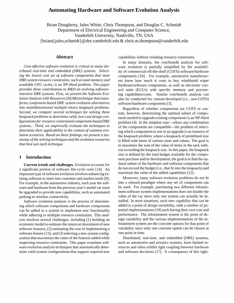
Figure 9 shows that regardless of the set count for theMMKP problems, the ASCENT solver derived a solutionmuch faster than LCS. This figure also shows that the re-

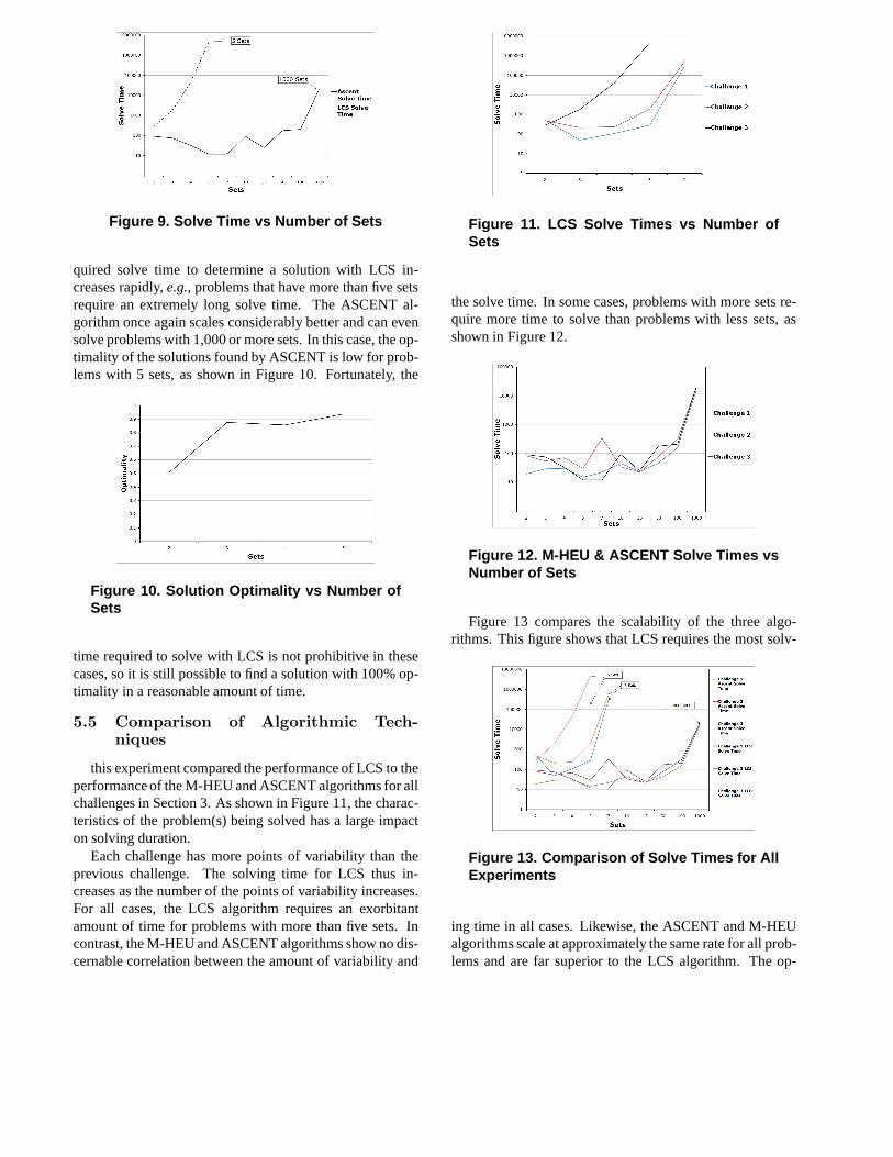
Figure 9. Solve Time vs Number of Sets

quired solve time to determine a solution with LCS in-creases rapidly,e.g., problems that have more than five setsrequire an extremely long solve time. The ASCENT al-gorithm once again scales considerably better and can evensolve problems with 1,000 or more sets. In this case, the op-timality of the solutions found by ASCENT is low for prob-lems with 5 sets, as shown in Figure 10. Fortunately, the

Figure 10. Solution Optimality vs Number ofSets

time required to solve with LCS is not prohibitive in thesecases, so it is still possible to find a solution with 100% op-timality in a reasonable amount of time.

5.5 Comparison of Algorithmic Tech-niques

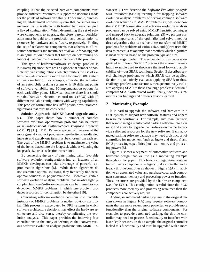
this experiment compared the performance of LCS to theperformance of the M-HEU and ASCENT algorithms for allchallenges in Section 3. As shown in Figure 11, the charac-teristics of the problem(s) being solved has a large impacton solving duration.

Each challenge has more points of variability than theprevious challenge. The solving time for LCS thus in-creases as the number of the points of variability increases.For all cases, the LCS algorithm requires an exorbitantamount of time for problems with more than five sets. Incontrast, the M-HEU and ASCENT algorithms show no dis-cernable correlation between the amount of variability and

Figure 11. LCS Solve Times vs Number ofSets

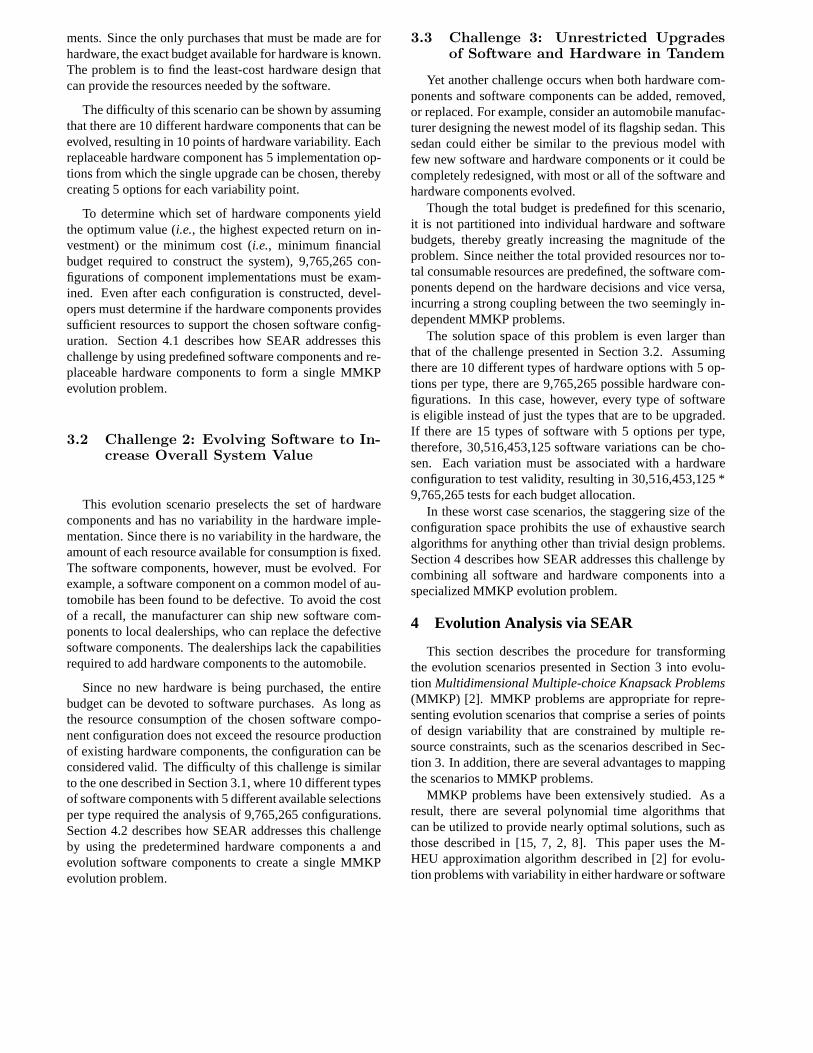
the solve time. In some cases, problems with more sets re-quire more time to solve than problems with less sets, asshown in Figure 12.

Figure 12. M-HEU & ASCENT Solve Times vsNumber of Sets

Figure 13 compares the scalability of the three algo-rithms. This figure shows that LCS requires the most solv-

Figure 13. Comparison of Solve Times for AllExperiments

ing time in all cases. Likewise, the ASCENT and M-HEUalgorithms scale at approximately the same rate for all prob-lems and are far superior to the LCS algorithm. The op-

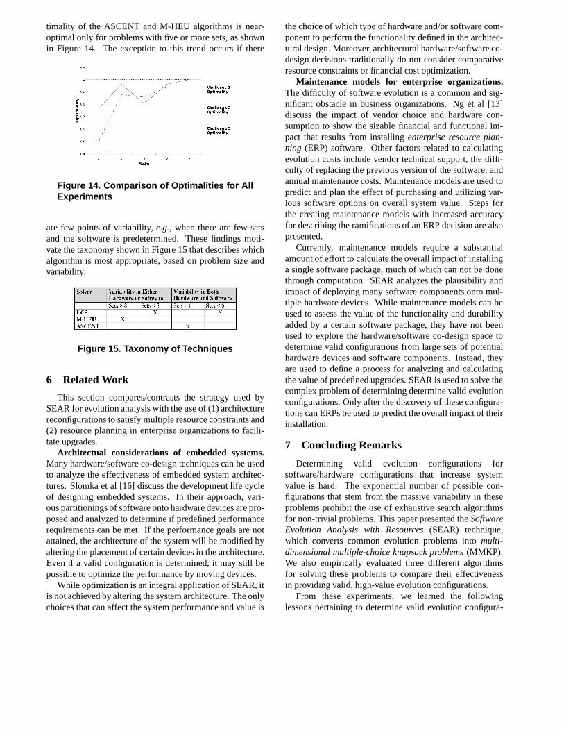
timality of the ASCENT and M-HEU algorithms is near-optimal only for problems with five or more sets, as shownin Figure 14. The exception to this trend occurs if there

Figure 14. Comparison of Optimalities for AllExperiments

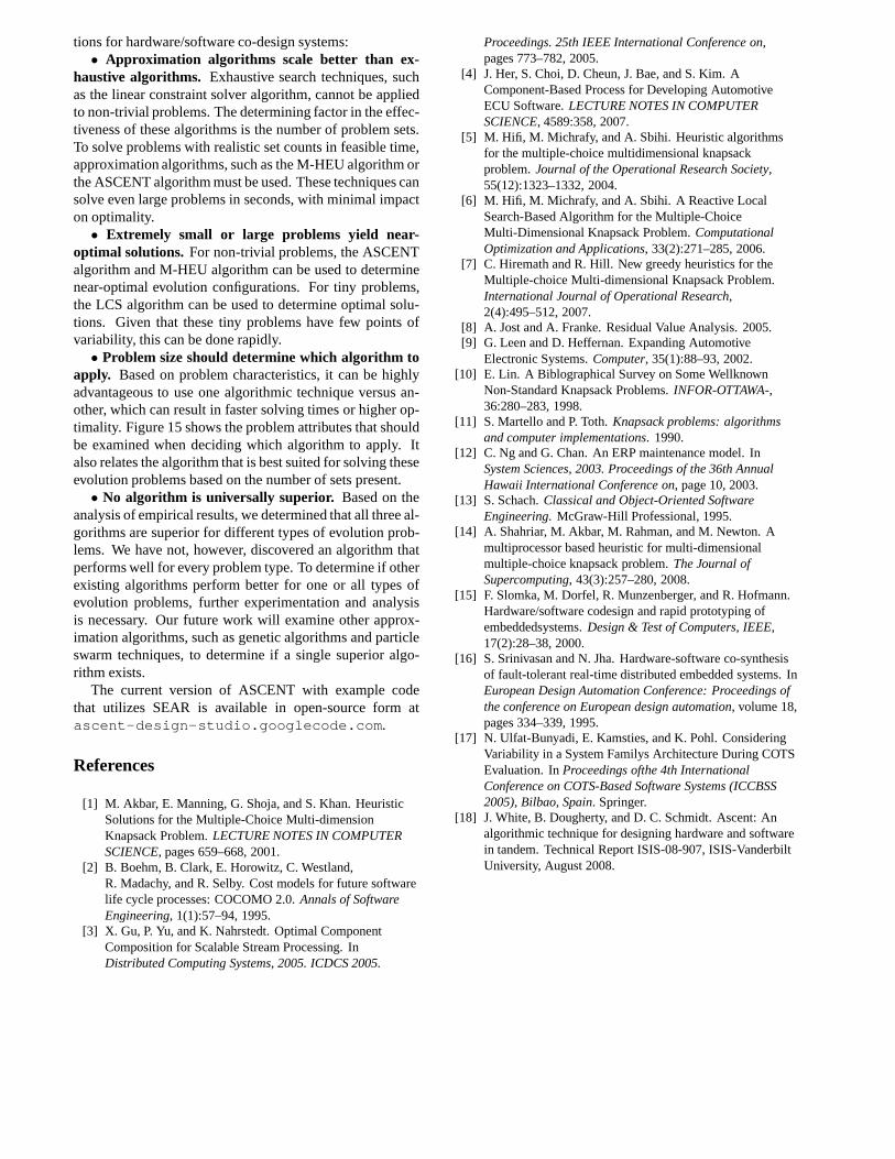
are few points of variability,e.g., when there are few setsand the software is predetermined. These findings moti-vate the taxonomy shown in Figure 15 that describes whichalgorithm is most appropriate, based on problem size andvariability.

Figure 15. Taxonomy of Techniques

6 Related Work

This section compares/contrasts the strategy used bySEAR for evolution analysis with the use of (1) architecturereconfigurations to satisfy multiple resource constraintsand(2) resource planning in enterprise organizations to facili-tate upgrades.

Architectual considerations of embedded systems.Many hardware/software co-design techniques can be usedto analyze the effectiveness of embedded system architec-tures. Slomka et al [16] discuss the development life cycleof designing embedded systems. In their approach, vari-ous partitionings of software onto hardware devices are pro-posed and analyzed to determine if predefined performancerequirements can be met. If the performance goals are notattained, the architecture of the system will be modified byaltering the placement of certain devices in the architecture.Even if a valid configuration is determined, it may still bepossible to optimize the performance by moving devices.

While optimization is an integral application of SEAR, itis not achieved by altering the system architecture. The onlychoices that can affect the system performance and value is

the choice of which type of hardware and/or software com-ponent to perform the functionality defined in the architec-tural design. Moreover, architectural hardware/softwareco-design decisions traditionally do not consider comparativeresource constraints or financial cost optimization.

Maintenance models for enterprise organizations.The difficulty of software evolution is a common and sig-nificant obstacle in business organizations. Ng et al [13]discuss the impact of vendor choice and hardware con-sumption to show the sizable financial and functional im-pact that results from installingenterprise resource plan-ning (ERP) software. Other factors related to calculatingevolution costs include vendor technical support, the diffi-culty of replacing the previous version of the software, andannual maintenance costs. Maintenance models are used topredict and plan the effect of purchasing and utilizing var-ious software options on overall system value. Steps forthe creating maintenance models with increased accuracyfor describing the ramifications of an ERP decision are alsopresented.

Currently, maintenance models require a substantialamount of effort to calculate the overall impact of installinga single software package, much of which can not be donethrough computation. SEAR analyzes the plausibility andimpact of deploying many software components onto mul-tiple hardware devices. While maintenance models can beused to assess the value of the functionality and durabilityadded by a certain software package, they have not beenused to explore the hardware/software co-design space todetermine valid configurations from large sets of potentialhardware devices and software components. Instead, theyare used to define a process for analyzing and calculatingthe value of predefined upgrades. SEAR is used to solve thecomplex problem of determining determine valid evolutionconfigurations. Only after the discovery of these configura-tions can ERPs be used to predict the overall impact of theirinstallation.

7 Concluding Remarks

Determining valid evolution configurations forsoftware/hardware configurations that increase systemvalue is hard. The exponential number of possible con-figurations that stem from the massive variability in theseproblems prohibit the use of exhaustive search algorithmsfor non-trivial problems. This paper presented theSoftwareEvolution Analysis with Resources(SEAR) technique,which converts common evolution problems intomulti-dimensional multiple-choice knapsack problems(MMKP).We also empirically evaluated three different algorithmsfor solving these problems to compare their effectivenessin providing valid, high-value evolution configurations.

From these experiments, we learned the followinglessons pertaining to determine valid evolution configura-

tions for hardware/software co-design systems:• Approximation algorithms scale better than ex-

haustive algorithms. Exhaustive search techniques, suchas the linear constraint solver algorithm, cannot be appliedto non-trivial problems. The determining factor in the effec-tiveness of these algorithms is the number of problem sets.To solve problems with realistic set counts in feasible time,approximation algorithms, such as the M-HEU algorithm orthe ASCENT algorithm must be used. These techniques cansolve even large problems in seconds, with minimal impacton optimality.

• Extremely small or large problems yield near-optimal solutions. For non-trivial problems, the ASCENTalgorithm and M-HEU algorithm can be used to determinenear-optimal evolution configurations. For tiny problems,the LCS algorithm can be used to determine optimal solu-tions. Given that these tiny problems have few points ofvariability, this can be done rapidly.

• Problem size should determine which algorithm toapply. Based on problem characteristics, it can be highlyadvantageous to use one algorithmic technique versus an-other, which can result in faster solving times or higher op-timality. Figure 15 shows the problem attributes that shouldbe examined when deciding which algorithm to apply. Italso relates the algorithm that is best suited for solving theseevolution problems based on the number of sets present.

• No algorithm is universally superior. Based on theanalysis of empirical results, we determined that all threeal-gorithms are superior for different types of evolution prob-lems. We have not, however, discovered an algorithm thatperforms well for every problem type. To determine if otherexisting algorithms perform better for one or all types ofevolution problems, further experimentation and analysisis necessary. Our future work will examine other approx-imation algorithms, such as genetic algorithms and particleswarm techniques, to determine if a single superior algo-rithm exists.

The current version of ASCENT with example codethat utilizes SEAR is available in open-source form atascent-design-studio.googlecode.com.

References

[1] M. Akbar, E. Manning, G. Shoja, and S. Khan. HeuristicSolutions for the Multiple-Choice Multi-dimensionKnapsack Problem.LECTURE NOTES IN COMPUTERSCIENCE, pages 659–668, 2001.

[2] B. Boehm, B. Clark, E. Horowitz, C. Westland,R. Madachy, and R. Selby. Cost models for future softwarelife cycle processes: COCOMO 2.0.Annals of SoftwareEngineering, 1(1):57–94, 1995.

[3] X. Gu, P. Yu, and K. Nahrstedt. Optimal ComponentComposition for Scalable Stream Processing. InDistributed Computing Systems, 2005. ICDCS 2005.

Proceedings. 25th IEEE International Conference on,pages 773–782, 2005.

[4] J. Her, S. Choi, D. Cheun, J. Bae, and S. Kim. AComponent-Based Process for Developing AutomotiveECU Software.LECTURE NOTES IN COMPUTERSCIENCE, 4589:358, 2007.

[5] M. Hifi, M. Michrafy, and A. Sbihi. Heuristic algorithmsfor the multiple-choice multidimensional knapsackproblem.Journal of the Operational Research Society,55(12):1323–1332, 2004.

[6] M. Hifi, M. Michrafy, and A. Sbihi. A Reactive LocalSearch-Based Algorithm for the Multiple-ChoiceMulti-Dimensional Knapsack Problem.ComputationalOptimization and Applications, 33(2):271–285, 2006.

[7] C. Hiremath and R. Hill. New greedy heuristics for theMultiple-choice Multi-dimensional Knapsack Problem.International Journal of Operational Research,2(4):495–512, 2007.

[8] A. Jost and A. Franke. Residual Value Analysis. 2005.[9] G. Leen and D. Heffernan. Expanding Automotive

Electronic Systems.Computer, 35(1):88–93, 2002.[10] E. Lin. A Biblographical Survey on Some Wellknown

Non-Standard Knapsack Problems.INFOR-OTTAWA-,36:280–283, 1998.

[11] S. Martello and P. Toth.Knapsack problems: algorithmsand computer implementations. 1990.

[12] C. Ng and G. Chan. An ERP maintenance model. InSystem Sciences, 2003. Proceedings of the 36th AnnualHawaii International Conference on, page 10, 2003.

[13] S. Schach.Classical and Object-Oriented SoftwareEngineering. McGraw-Hill Professional, 1995.

[14] A. Shahriar, M. Akbar, M. Rahman, and M. Newton. Amultiprocessor based heuristic for multi-dimensionalmultiple-choice knapsack problem.The Journal ofSupercomputing, 43(3):257–280, 2008.

[15] F. Slomka, M. Dorfel, R. Munzenberger, and R. Hofmann.Hardware/software codesign and rapid prototyping ofembeddedsystems.Design & Test of Computers, IEEE,17(2):28–38, 2000.

[16] S. Srinivasan and N. Jha. Hardware-software co-synthesisof fault-tolerant real-time distributed embedded systems. InEuropean Design Automation Conference: Proceedings ofthe conference on European design automation, volume 18,pages 334–339, 1995.

[17] N. Ulfat-Bunyadi, E. Kamsties, and K. Pohl. ConsideringVariability in a System Familys Architecture During COTSEvaluation. InProceedings ofthe 4th InternationalConference on COTS-Based Software Systems (ICCBSS2005), Bilbao, Spain. Springer.

[18] J. White, B. Dougherty, and D. C. Schmidt. Ascent: Analgorithmic technique for designing hardware and softwarein tandem. Technical Report ISIS-08-907, ISIS-VanderbiltUniversity, August 2008.