1

Version 2 - Submitted December 31, 1998 for EUROGEN workshop in Jyvdskyld, Finland on May 30 – June 3, 1999. 9,987 words – 28 pages of text plus 17 figures.

Automatic Synthesis of the Topology and Sizing for Analog Electrical Circuits using Genetic Programming F. H BENNETT1 III, M. A. KEANE2, D. ANDRE3, AND J. R. KOZA4

1Genetic Programming Inc. Los Altos, California USA 2Econometrics Inc. Chicago, Illinois USA 3University of California Berkeley, California USA 4Stanford University Stanford, California USA

1. INTRODUCTION Design is a major activity of practicing engineers. The design process entails creation of a complex structure to satisfy user-defined requirements. Since the design process typically entails tradeoffs between competing considerations, the end product of the process is usually a satisfactory and compliant design as opposed to a perfect design. Design is usually viewed as requiring creativity and human intelligence. Consequently, the field of design is a source of challenging problems for automated techniques of machine intelligence. In particular, design problems are useful for determining whether an automated technique can produce results that are competitive with human-produced results.

The design (synthesis) of analog electrical circuits is especially challenging. The design process for analog circuits

2

begins with a high-level description of the circuit's desired behavior and characteristics and includes creation of both the topology and the sizing of a satisfactory circuit. The topology of a circuit involves specification of the gross number of components in the circuit, the type of each component (e.g., a capacitor), and a netlist specifying where each of a component's leads are to be connected. Sizing involves specification of the values (typically numerical) of each component. Since the design process typically involves tradeoffs between competing considerations, the end product of the process is usually a satisfactory and compliant design as opposed to a perfect design.

Although considerable progress has been made in automating the synthesis of certain categories of purely digital circuits, the synthesis of analog circuits and mixed analog-digital circuitshas not proved to be as amenable to automation [30]. Until recently, there has been no general technique for automatically creating the topology and sizing for an entire analog electrical circuit from a high-level statement of the design goals of the circuit. Describing "the analog dilemma," O. Aaserud and I. Ring Nielsen [1] noted

"Analog designers are few and far between. In contrast to digital design, most of the analog circuits are still handcrafted by the experts or so-called 'zahs' of analog design. The design process is characterized by a combination of experience and intuition and requires a thorough knowledge of the process characteristics and the detailed specifications of the actual product.

"Analog circuit design is known to be a knowledge-intensive, multiphase, iterative task, which usually stretches over a significant period of time and is performed by designers with a large portfolio of skills. It is therefore considered by many to be a form of art rather than a science."

There has been extensive previous work (surveyed in [23]) on the problem of automated circuit design (synthesis) using simulated annealing, artificial intelligence, and other techniques, including work employing genetic algorithms [11, 27, 34].

This paper presents a uniform approach to the automatic synthesis of both the topology and sizing of analog electrical circuits. Section 2 presents seven design problems involving prototypical analog circuits. Section 3 describes genetic programming. Section 4 details the circuit-constructing functions used in applying genetic programming to the problem of analog circuit synthesis. Section 5 presents the preparatory steps required for applying genetic programming to a particular design problem. Section 6 shows the results for the seven problems. Section 7 cites other circuits that have been designed by genetic programming.

3

2. SEVEN PROBLEMS OF ANALOG DESIGN

This paper applies genetic programming to an illustrative suite of seven problems of analog circuit design. The circuits comprise a variety of types of components, including transistors, diodes, resistors, inductors, and capacitors. The circuits have varying numbers of inputs and outputs. They circuits encompass both passive and active circuits.

(1) Design a one-input, one-output lowpass filter composed of capacitors and inductors that passes all frequencies below 1,000 Hz and suppresses all frequencies above 2,000 Hz.

(2) Design a one-input, one-output highpass filter composed of capacitors and inductors that suppresses all frequencies below 1,000 Hz and passes all frequencies above 2,000 Hz.

(3) Design a one-input, one-output bandpass filter composed of capacitors and inductors that passes all frequencies between 500 Hz and 1,000 Hz and suppresses frequencies that are less than 250 Hz and greater than 2,000 Hz.

(4) Design a one-input, one-output frequency-measuring circuit that is composed of capacitors and inductors whose output in millivolts (from 1 millivolt to 1,000 millivolts) is proportional to the frequency of an incoming signal (between 1 Hz and 100,000 Hz).

(5) Design a one-input, one-output computational circuit that is composed of transistors, diodes, resistors, and capacitors and that produces an output voltage equal to the square root of its input voltage.

(6) Design a two-input, one-output time-optimal robot controller circuit that is composed of the above components and that navigates a constant-speed autonomous mobile robot (with nonzero turning radius) to an arbitrary destination in minimal time.

(7) Design a one-input, one-output amplifier composed of the above components and that delivers amplification of 60 dB (i.e., 1,000 to 1) with low distortion and low bias.

The above seven prototypical circuits are representative of analog circuits that are in widespread use. Filters extract specified ranges of frequencies from electrical signals and amplifiers enhance the amplitude of signal. Amplifiers are used to increase the amplitude of an incoming signal. Analog computational circuits are used to perform real-time mathematical calculations on signals. Embedded controllers are used to control the operation of numerous automatic devices.

3. BACKGROUND ON GENETIC PROGRAMMING

Genetic programming is a biologically inspired, domain-independent method that automatically creates a computer program from a high-level statement of a problem's requirements. Genetic programming is an extension of the

4

genetic algorithm described in John Holland's pioneering book Adaptation in Natural and Artificial Systems [13]. In genetic programming, the genetic algorithm operates on a population of computer programs of varying sizes and shapes [18, 26].

Starting with a primordial ooze of thousands of randomly created computer programs, genetic programming progressively breeds a population of computer programs over a series of generations. Genetic programming applies the Darwinian principle of survival of the fittest, analogs of naturally occurring operations such as sexual recombination (crossover), mutation, gene duplication, and gene deletion, and certain mechanisms of developmental biology. The computer programs are compositions of functions (e.g., arithmetic operations, conditional operators, problem-specific functions) and terminals (e.g., external inputs, constants, zero-argument functions). The programs may be thought of as trees whose points are labeled with the functions and whose leaves are labeled with the terminals.

Genetic programming breeds computer programs to solve problems by executing the following three steps:

(1) Randomly create an initial population of individual computer programs. (2) Iteratively perform the following substeps (called a generation) on the population of programs until the termination criterion has been satisfied:

(a) Assign a fitness value to each individual program in the population using the fitness measure. (b) Create a new population of individual programs by applying the following three genetic operations. The genetic operations are applied to one or two individuals in the population selected with a probability based on fitness (with reselection allowed).

(i) Reproduce an existing individual by copying it into the new population. (ii) Create two new individual programs from two existing parental individuals by genetically recombining subtrees from each program using the crossover operation at randomly chosen crossover points in the parental individuals. (iii) Create a new individual from an existing parental individual by randomly mutating one randomly chosen subtree of the parental individual.

(3) Designate the individual computer program that is identified by the method of result designation (e.g., the best-so-far individual) as the result of the run of genetic programming. This result may represent a solution (or an approximate solution) to the problem. The hierarchical character and the dynamic variability of the

computer programs that are developed along the way to a solution are important features of genetic programming. It is

5

often difficult and unnatural to try to specify or restrict the size and shape of the eventual solution in advance.

Automated programming requires some hierarchical mechanism to exploit, by reuse and parameterization, the regularities, symmetries, homogeneities, similarities, patterns, and modularities inherent in problem environments. Subroutines do this in ordinary computer programs. Automatically defined functions [19,. 20] can be implemented within the context of genetic programming by establishing a constrained syntactic structure for the individual programs in the population. Each multi-part program in the population contains one (or more) function-defining branches and one (or more) main result-producing branches. The result-producing branch usually has the ability to call one or more of the automatically defined functions. A function-defining branch may have the ability to refer hierarchically to other already-defined automatically defined functions.

Since each individual program in the population of this example consists of function-defining branch(es) and result-producing branch(es), the initial random generation is created so that every individual program in the population has this particular constrained syntactic structure. Since a constrained syntactic structure is involved, crossover is performed so as to preserve this syntactic structure in all offspring.

Architecture-altering operations enhance genetic programming with automatically defined functions by providing a way to automatically determine the number of such automatically defined functions, the number of arguments that each automatically defined function possesses, and the nature of the hierarchical references, if any, among such automatically defined functions [21]. These operations include branch duplication, argument duplication, branch creation, argument creation, branch deletion, and argument deletion. The architecture-altering operations are motivated by the naturally occurring mechanism of gene duplication that creates new proteins (and hence new structures and new behaviors in living things) [28].

Genetic programming has been applied to numerous problems in fields such as system identification, control, classification, design, optimization, and automatic programming. Current research is described in [3, 4, 5, 16, 22, 23, 24, 25, 32] and on the World Wide Web at www.genetic-programming.org.

4. APPLYING GENETIC PROGRAMMING TO ANALOG CIRCUIT SYNTHESIS

Genetic programming can be applied to the problem of synthesizing circuits if a mapping is established between the program trees (rooted, point-labeled trees – that is, acyclic

6

graphs – with ordered branches) used in genetic programming and the labeled cyclic graphs germane to electrical circuits. The principles of developmental biology and work on applying genetic algorithms and genetic programming to evolve neural networks [12, 17] provide the motivation for mapping trees into circuits by means of a developmental process that begins with a simple embryo. The initial circuit typically includes fixed wires that connect the inputs and outputs of the particular circuit being designed and certain fixed components (such as source and load resistors). Until these wires are modified, the initial circuit does not produce interesting output. An electrical circuit is developed by progressively applying the functions in a circuit-constructing program tree to the modifiable wires of the embryo (and, during the developmental process, to new components and modifiable wires).

An electrical circuit is created by executing the functions in a circuit-constructing program tree. The functions are progressively applied in a developmental process to the embryo and its successors until all of the functions in the program tree are executed. That is, the functions in the circuit-constructing program tree progressively side-effect the embryo and its successors until a fully developed circuit eventually emerges. The functions are applied in a breadth-first order.

The functions in the circuit-constructing program trees are divided into five categories: (1) topology-modifying functions that alter the circuit topology, (2) component-creating functions that insert components into the circuit, (3) development-controlling functions that control the development process by which the embryo and its successors is changed into a fully developed circuit, (4) arithmetic-performing functions that appear in subtrees as argument(s) to the component-creating functions and specify the numerical value of the component, and (5) automatically defined functions that appear in the function-defining branches and potentially enable certain substructures of the circuit to be reused (with parameterization).

Each branch of the program tree is created in accordance with a constrained syntactic structure. Each branch is composed of topology-modifying functions, component-creating functions, development-controlling functions, and terminals. Component-creating functions typically have one arithmetic-performing subtree, while topology-modifying functions, and development-controlling functions do not. Component-creating functions and topology-modifying functions are internal points of their branches and possess one or more arguments (construction-continuing subtrees) that continue the developmental process. The syntactic validity of this constrained syntactic structure is preserved using structure-preserving crossover with point typing. For details, see [23].

7

4.1. The Initial Circuit An electrical circuit is created by executing a circuit-constructing program tree that contains various component-creating, topology-modifying, and development-controlling functions. Each circuit-constructing program tree in the population creates one circuit.

Fig. 1 shows a one-input, one-output initial circuit in which VSOURCE is the input signal and VOUT is the output signal (the probe point). The circuit is driven by an incoming alternating circuit source VSOURCE. There is a fixed load resistor RLOAD and a fixed source resistor RSOURCE. All of the foregoing items are called the test fixture. The test fixture is fixed. It provides a means for testing individual evolved circuits. An embryo is embedded within the test fixture. The embryo contains one or more modifiable wires or modifiable components. In the figure, there a modifiable wire Z0 between nodes 2 and 3. All development originates from modifiable wires or modifiable components.

---All figures are at end of paper and are also provided as a separate files in EPS format

Fig. 1 One-input, one-output embryo

4.2. Component-Creating Functions The component-creating functions insert a component into the developing circuit and assign component value(s) to the component.

Each component-creating function has a writing head that points to an associated highlighted component in the developing circuit and modifies that component in a specified manner. The construction-continuing subtree of each component-creating function points to a successor function or terminal in the circuit-constructing program tree.

The arithmetic-performing subtree of a component-creating function consists of a composition of arithmetic functions (addition and subtraction) and random constants (in the range -1.000 to +1.000). The arithmetic-performing subtree specifies the numerical value of a component by returning a floating-point value that is interpreted on a logarithmic scale as the value for the component in a range of 10 orders of magnitude (using a unit of measure that is appropriate for the particular type of component).

8

The two-argument resistor-creating R function causes the highlighted component to be changed into a resistor. The value of the resistor in kilo Ohms is specified by its arithmetic-performing subtree.

Fig. 2 shows a modifiable wire Z0 connecting nodes 1 and 2 of a partial circuit containing four capacitors (C2, C3, C4, and C5). The circle indicates that Z0 has a writing head (i.e., is the highlighted component and that Z0 is subject to subsequent modification). Fig. 3 shows the result of applying the R function to the modifiable wire Z0 of fig. 2. The circle indicates that the newly created R1 has a writing head so that R1 remains subject to subsequent modification.

Fig. 2 Modifiable wire Z0

Fig. 3 Result of applying the R function.

Similarly, the two-argument capacitor-creating C function

causes the highlighted component to be changed into a capacitor whose value in micro-Farads is specified by its arithmetic-performing subtree. In addition, the two-argument inductor-creating L function causes the highlighted component to be changed into an inductor whose value in micro-Henrys is specified by its arithmetic-performing subtree.

The one-argument Q_D_PNP diode-creating function causes a diode to be inserted in lieu of the highlighted component. This function has only one argument because there is no numerical value associated with a diode and thus no arithmetic-performing subtree. In practice, the diode is implemented here using a pnp transistor whose collector and base are connected to each other. The Q_D_NPN function inserts a diode using an npn transistor in a similar manner.

There are also six one-argument transistor-creating functions (Q_POS_COLL_NPN, Q_GND_EMIT_NPN, Q_NEG_EMIT_NPN, Q_GND_EMIT_PNP, Q_POS_EMIT_PNP, Q_NEG_COLL_PNP) that insert a bipolar junction transistor in lieu of the highlighted component and that directly connect the collector or emitter of the newly created transistor to a fixed point of the circuit (the positive power supply, ground, or the negative power supply). For example, the Q_POS_COLL_NPN function inserts a bipolar junction transistor whose collector is connected to the positive power supply.

9

Each of the functions in the family of six different three-argument transistor-creating Q_3_NPN functions causes an npn bipolar junction transistor to be inserted in place of the highlighted component and one of the nodes to which the highlighted component is connected. The Q_3_NPN function creates five new nodes and three modifiable wires. There is no writing head on the new transistor, but there is a writing head on each of the three new modifiable wires. There are 12 members (called Q_3_NPN0, ..., Q_3_NPN11) in this family of functions because there are two choices of nodes (1 and 2) to be bifurcated and then there are six ways of attaching the transistor's base, collector, and emitter after the bifurcation. Similarly the family of 12 Q_3_PNP functions causes a pnp bipolar junction transistor to be inserted.

4.3. Topology-Modifying Functions Each topology-modifying function in a program tree points to an associated highlighted component and modifies the topology of the developing circuit.

The three-argument SERIES division function creates a series composition of the highlighted component (with a writing head), a copy of it (with a writing head), one new modifiable wire (with a writing head), and two new nodes.

The four-argument PARALLEL0 parallel division function creates a parallel composition consisting of the original highlighted component (with a writing head), a copy of it (with a writing head), two new modifiable wires (each with a writing head), and two new nodes. There are potentially two topologically distinct outcomes of a parallel division. Since we want the outcome of all circuit-constructing functions to be deterministic, there are two members (called PARALLEL0 and PARALLEL1) in the PARALLEL family of topology-modifying functions. The two functions operate differently depending on degree and numbering of the preexisting components in the developing circuit. The use of the two functions breaks the symmetry between the potentially distinct outcomes. Fig. 4 shows the result of applying PARALLEL0 to the resistor R1 from fig. 3. Modifiable resistors R1 and R7 and modifiable wires Z6 and Z8 are each linked to the top-most function in one of the four construction-continuing subtrees of the PARALLEL0 function.

Fig. 4 Result of the PARALLEL0 function

10

The reader is referred to [23] for a detailed description of the operation of the PARALLEL0 and PARALLEL1 functions (and other functions mentioned herein).

If desired, other topology-modifying functions may be defined to create the Y-shaped divisions and ∆-shaped divisions that are frequently seen in human-designed circuits.

The one-argument polarity-reversing FLIP function reverses the polarity of the highlighted component.

There are six three-argument functions (T_GND_0, T_GND_1, T_POS_0, T_POS_1, T_NEG_0, T_NEG_1) that insert two new nodes and two new modifiable wires, and then make a connection to ground, positive power supply, or negative power supply, respectively.

There are two three-argument functions (PAIR_CONNECT_0 and PAIR_CONNECT_1) that enable distant parts of a circuit to be connected together. The first PAIR_CONNECT to occur in the development of a circuit creates two new wires, two new nodes, and one temporary port. The next PAIR_CONNECT creates two new wires and one new node, connects the temporary port to the end of one of these new wires, and then removes the temporary port.

If desired, numbered vias can be created to provide connectivity between distant points of the circuit by using a three-argument VIA function.

The zero-argument SAFE_CUT function causes the highlighted component to be removed from the circuit provided that the degree of the nodes at both ends of the highlighted component is three (i.e., no dangling components or wires are created).

4.4. Development-Controlling Functions The one-argument NOOP ("No Operation") function has no effect on the modifiable wire or modifiable component with which it is associated; however, it has the effect of delaying activity on the developmental path on which it appears in relation to other developmental paths in the overall circuit-constructing program tree. The zero-argument END function makes the modifiable wire or modifiable component with which it is associated into a non-modifiable wire or component (thereby ending a particular developmental path).

4.5. Example of Developmental Process Fig. 5 is an illustrative circuit-constructing program tree shown as a rooted, point-labeled tree with ordered branches. The overall program consists of two main result-producing branches joined by a connective LIST function (labeled 1 in the figure). The first (left) result-producing branch is rooted at the capacitor-creating C function (labeled 2). The second result-producing branch is rooted at the polarity-reversing FLIP function (labeled 3). This figure also contains four occurrences of the

11

inductor-creating L function (at 17, 11, 20, and 12). The figure contains two occurrences of the topology-modifying SERIES function (at 5 and 10). The figure also contains five occurrences of the development-controlling END function (at 15, 25, 27, 31, and 22) and one occurrence of the development-controlling "no operation" NOP function (at 6). There is a seven-point arithmetic-performing subtree at 4 under the capacitor-creating C function at 4. Similarly, there is a three-point arithmetic-performing subtree at 19 under the inductor-creating L function at 11. There are also one-point arithmetic-performing subtrees (i.e., constants) at 26, 30, and 21. Additional details can be found in [23].

Fig. 5 Illustrative circuit-constructing program tree.

5. PREPARATORY STEPS Before applying genetic programming to a problem of circuit design, seven major preparatory steps are required: (1) identify the initial circuit, (2) determine the architecture of the circuit-constructing program trees, (3) identify the primitive functions of the program trees, (4) identify the terminals of the program trees, (5) create the fitness measure, (6) choose control parameters for the run, and (7) determine the termination criterion and method of result designation.

5.1. Initial Circuit The initial circuit used on a particular problem depends on the circuit's number of inputs and outputs. All development originates from the modifiable wires of the embryo within the initial circuit. .

An embryo with two modifiable wires (Z0 and Z1) was used for the one-input, one-output lowpass filter, highpass filter, bandpass filter, and frequency-measuring circuits.

The robot controller circuit has two inputs (VSOURCE1 and VSOURCE2) representing the two-dimensional position of the target point. Therefore, this problem requires a different initial circuit than that used above. Both voltage inputs require their own separate source resistor (RSOURCE1 and RSOURCE2). The embryo for the robot controller circuit has three modifiable wires (Z0, Z1, and Z2) in order to provide full connectivity between the two inputs and the one output.

In some problems, such as the amplifier, the embryo contains additional fixed components (as detailed in [23]).

For historical reasons, an embryo with one modifiable wire was used for the computational circuit. However, an embryo with two modifiable wires could have been used on these problems and an embryo with one modifiable wire could have

12

been used on the lowpass filter, highpass filter, and bandpass filter, and frequency-measuring circuits.

5.2. Program Architecture Since there is one result-producing branch in the program tree for each modifiable wire in the embryo, the architecture of each circuit-constructing program tree depends on the embryo. One result-producing branch was used for the computational circuit; two were used for lowpass, highpass, and bandpass filter, problems; and three were used for the robot controller and amplifier.

The architecture of each circuit-constructing program tree also depends on the use, if any, of automatically defined functions. Automatically defined functions provide a mechanism enabling certain substructures to be reused and are described in detail in [23]. Automatically defined functions and architecture-altering operations were used in the robot controller, and amplifier. For these problems, each program in the initial population of programs had a uniform architecture with no automatically defined functions. In later generations, the number of automatically defined functions, if any, emerged as a consequence of the architecture-altering operations (also described in [23]).

5.3. Function and Terminal Sets The function set for each design problem depends on the type of electrical components that are to be used for constructing the circuit.

For the problems of synthesizing a lowpass, highpass, and bandpass filter and the problem of synthesizing a frequency-measuring circuit, the function set included two component-creating functions (for inductors and capacitors), topology-modifying functions (for series and parallel divisions and for flipping components), one development-controlling function (“no operation”), functions for creating a via to ground, and functions for connecting pairs of points. That is, the function set, Fccs-initial, for each construction-continuing subtree was Fccs-initial = L, C, SERIES, PARALLEL0, PARALLEL1,

FLIP, NOOP, T_GND_0, T_GND_1, PAIR_CONNECT_0, PAIR_CONNECT_1.

Capacitors, resistors, diodes, and transistors were used for the computational circuit, the robot controller, and the amplifier. In addition, the function set also included functions to provide connectivity to the positive and negative power supplies (in order to provide a source of energy for the transistors). Thus, the function set, Fccs-initial, for each construction-continuing subtree was Fccs-initial = R, C, SERIES, PARALLEL0, PARALLEL1,

FLIP, NOOP, T_GND_0, T_GND_1, T_POS_0, T_POS_1, T_NEG_0, T_NEG_1, PAIR_CONNECT_0, PAIR_CONNECT_1, Q_D_NPN, Q_D_PNP,

13

Q_3_NPN0, ..., Q_3_NPN11, Q_3_PNP0, ..., Q_3_PNP11, Q_POS_COLL_NPN, Q_GND_EMIT_NPN, Q_NEG_EMIT_NPN, Q_GND_EMIT_PNP, Q_POS_EMIT_PNP, Q_NEG_COLL_PNP.

For the npn transistors, the Q2N3904 model was used. For pnp transistors, the Q2N3906 model was used.

The initial terminal set, Tccs-initial, for each construction-continuing subtree was Tccs-initial = END, SAFE_CUT.

The initial terminal set, Taps-initial, for each arithmetic-performing subtree consisted of Taps-initial = ℜ, where ℜ represents floating-point random constants from –1.0 to +1.0.

The function set, Faps, for each arithmetic-performing subtree was, Faps = +, -.

The terminal and function sets were identical for all result-producing branches for a particular problem.

For the lowpass filter, highpass filter, and bandpass filter, there was no need for functions to provide connectivity to the positive and negative power supplies.

For the robot controller and the amplifier, the architecture-altering operations were used and the set of potential new functions, Fpotential, was Fpotential = ADF0, ADF1, ....

The set of potential new terminals, Tpotential, for the automatically defined functions was Tpotential = ARG0.

The architecture-altering operations change the function set, Fccs for each construction-continuing subtree of all three result-producing branches and the function-defining branches, so that Fccs = Fccs-initial ≈ Fpotential.

The architecture-altering operations generally change the terminal set for automatically defined functions, Taps-adf, for each arithmetic-performing subtree, so that Taps-adf = Taps-initial ≈ Tpotential.

5.4. Fitness Measure The evolutionary process is driven by the fitness measure. Each individual computer program in the population is executed and then evaluated, using the fitness measure. The nature of the fitness measure varies with the problem. The high-level statement of desired circuit behavior is translated into a well-defined measurable quantity that can be used by genetic programming to guide the evolutionary process. The evaluation of each individual circuit-constructing program tree in the

14

population begins with its execution. This execution progressively applies the functions in each program tree to the initial circuit, thereby creating a fully developed circuit. A netlist is created that identifies each component of the developed circuit, the nodes to which each component is connected, and the value of each component. The netlist becomes the input to our modified version of the 217,000-line SPICE (Simulation Program with Integrated Circuit Emphasis) simulation program [29]. SPICE then determines the behavior of the circuit. It was necessary to make considerable modifications in SPICE so that it could run as a submodule within the genetic programming system. 5.4.1. Fitness Measure for the Lowpass Filter A simple filter is a one-input, one-output electronic circuit that receives a signal as its input and passes the frequency components of the incoming signal that lie in a specified range (called the passband) while suppressing the frequency components that lie in all other frequency ranges (the stopband).

The desired lowpass LC filter has a passband below 1,000 Hz and a stopband above 2,000 Hz. The circuit is driven by an incoming AC voltage source with a 2 volt amplitude.

The attenuation of the filter is defined in terms of the output signal relative to the reference voltage (half of 2 volt here). A decibel is a unitless measure of relative voltage that is defined as 20 times the common (base 10) logarithm of the ratio between the voltage at a particular probe point and a reference voltage.

In this problem, a voltage in the passband of exactly 1 volt and a voltage in the stopband of exactly 0 volts is regarded as ideal. The (preferably small) variation within the passband is called the passband ripple. Similarly, the incoming signal is never fully reduced to zero in the stopband of an actual filter. The (preferably small) variation within the stopband is called the stopband ripple. A voltage in the passband of between 970 millivolts and 1 volt (i.e., a passband ripple of 30 millivolts or less) and a voltage in the stopband of between 0 volts and 1 millivolts (i.e., a stopband ripple of 1 millivolts or less) is regarded as acceptable. Any voltage lower than 970 millivolts in the passband and any voltage above 1 millivolts in the stopband is regarded as unacceptable.

A fifth-order elliptic (Cauer) filter with a modular angle Θ of 30 degrees (i.e., the arcsin of the ratio of the boundaries of the passband and stopband) and a reflection coefficient ρ of 24.3% is required to satisfy these design goals [35].

Since the high-level statement of behavior for the desired circuit is expressed in terms of frequencies, the voltage VOUT is measured in the frequency domain. SPICE performs an AC small signal analysis and reports the circuit's behavior over five decades (between 1 Hz and 100,000 Hz) with each decade being divided into 20 parts (using a logarithmic scale), so that there are a total of 101 fitness cases.

15

Fitness is measured in terms of the sum over these cases of the absolute weighted deviation between the actual value of the voltage that is produced by the circuit at the probe point VOUT and the target value for voltage. The smaller the value of fitness, the better. A fitness of zero represents an (unattainable) ideal filter.

Specifically, the standardized fitness is

))()),100

0((()( ifdifi ifdWtF ∑

==

where fi is the frequency of fitness case i; d(x) is the absolute value of the difference between the target and observed values at frequency x; and W(y,x) is the weighting for difference y at frequency x.

The fitness measure is designed to not penalize ideal values, to slightly penalize every acceptable deviation, and to heavily penalize every unacceptable deviation. Specifically, the procedure for each of the 61 points in the 3-decade interval between 1 Hz and 1,000 Hz for the intended passband is as follows:

• If the voltage equals the ideal value of 1.0 volt in this interval, the deviation is 0.0. • If the voltage is between 970 millivolts and 1 volt, the absolute value of the deviation from 1 volt is weighted by a factor of 1.0. • If the voltage is less than 970 millivolts, the absolute value of the deviation from 1 volt is weighted by a factor of 10.0. The acceptable and unacceptable deviations for each of the

35 points from 2,000 Hz to 100,000 Hz in the intended stopband are similarly weighed (by 1.0 or 10.0) based on the amount of deviation from the ideal voltage of 0 volts and the acceptable deviation of 1 millivolts.

For each of the five "don't care" points between 1,000 and 2,000 Hz, the deviation is deemed to be zero.

The number of “hits” for this problem (and all other problems herein) is defined as the number of fitness cases for which the voltage is acceptable or ideal or that lie in the "don't care" band (for a filter).

Many of the random initial circuits and many that are created by the crossover and mutation operations in subsequent generations cannot be simulated by SPICE. These circuits receive a high penalty value of fitness (108) and become the worst-of-generation programs for each generation. For details, see [23]. 5.4.2. Fitness Measure for the Highpass Filter The fitness cases for the highpass filter are the same 101 points in the five decades of frequency between 1 Hz and 100,000 Hz as for the lowpass filter. The fitness measure is substantially the same as that for the lowpass filter problem above, except that the locations of the passband and stopband are reversed. Notice that

16

the only difference in the seven preparatory steps for a highpass filter versus a lowpass filter is this change in the fitness measure. 5.4.3. Fitness Measure for the Bandpass Filter

The fitness cases for the bandpass filter are the same 101 points in the five decades of frequency between 1 Hz and 100,000 Hz as for the lowpass filter. The acceptable deviation in the desired passband between 500 Hz and 1,000 Hz is 30 millivolts (i.e., the same as for the passband of the lowpass and highpass filters above). The acceptable deviation in the two stopbands (i.e., between 1 Hz and 250 Hz and between 2,000 Hz and 100,000 Hz is 1 millivolt1 (i.e., the same as for the stopband of the lowpass and highpass filters above). Again, notice that the only difference in the seven preparatory steps for a bandpass filter versus a lowpass or highpass filter is a change in the fitness measure. 5.4.4. Fitness Measure for Frequency-Measuring

Circuit The fitness cases for the frequency-measuring circuit are the same 101 points in the five decades of frequency (on a logarithmic scale) between 1 Hz and 100,000 Hz as for the lowpass and lowpass filters. The circuit's output in millivolts (from 1 millivolt to 1,000 millivolts) is intended to be proportional to the frequency of an incoming signal (between 1 Hz and 100,000 Hz). Fitness is the sum, over the 101 fitness cases, of the absolute value of the difference between the circuit's actual output and the desired output voltage. 5.4.5. Fitness Measure for the Computational Circuit SPICE is called to perform a DC sweep analysis at 21 equidistant voltages between –250 millivolts and +250 millivolts. Fitness is the sum, over these 21 fitness cases, of the absolute weighted deviation between the actual value of the voltage that is produced by the circuit and the target value for voltage. For details, see [23]. 5.4.6. Fitness Measure for the Robot Controller

Circuit The fitness of a robot controller was evaluated using 72 randomly chosen fitness cases each representing different two-dimensional target points. Fitness is the sum, over the 72 fitness cases, of the travel times of the robot to the target point. If the robot came within a capture radius of 0.28 meters of its target point before the end of the 80 time steps allowed for a particular fitness case, the contribution to fitness for that fitness case was the actual time. However, if the robot failed to come within the capture radius during the 80 time steps, the contribution to fitness was a penalty value of 0.160 hours (i.e., double the worst possible time).

The two voltage inputs to the circuit represents the two-dimensional location of the target point. SPICE performs a nested DC sweep, which provides a way to simulate the DC

17

behavior of a circuit with two inputs. The nested DC sweep resembles a nested pair of FOR loops in a computer program in that both of the loops have a starting value for the voltage, an increment, and an ending value for the voltage. For each voltage value in the outer loop, the inner loop simulates the behavior of the circuit by stepping through its range of voltages. Specifically, the starting value for voltage is –4 volt, the step size is 0.2 volt, and the ending value is +4 volt. These values correspond to the dimensions of the robot's world of 64 square meters extending 4 meters in each of the four directions from the origin of a coordinate system (i.e., 1 volt equals 1 meter). For details, see [23]. 5.4.7. Fitness Measure for the 60 dB Amplifier SPICE was requested to perform a DC sweep analysis to determine the circuit's response for several different DC input voltages. An ideal inverting amplifier circuit would receive the DC input, invert it, and multiply it by the amplification factor. A circuit is flawed to the extent that it does not achieve the desired amplification, the output signal is not perfectly centered on 0 volts(i.e., it is biased), or the DC response is not linear. Fitness is calculated by summing an amplification penalty, a bias penalty, and two non-linearity penalties – each derived from these five DC outputs. For details, see [6].

5.5. Control Parameters The population size, M, was 1,400,000 for the bandpass filter problem and 640,000 for all other problems.

5.6. Implementation on Parallel Computer All problems except the bandpass filter were run on a medium-grained parallel Parsytec computer system consisting of 64 80-MHz PowerPC 601 processors arranged in an 8 by 8 toroidal mesh with a host PC Pentium type computer. The bandpass filter problem was run on a medium-grained parallel Beowulf-style [33] arranged in an 7 by 10 toroidal mesh with a host Alpha computer. The distributed genetic algorithm [2] was used. When the population size was 640,000, Q = 10,000 at each of the D = 64 demes (semi-isolated subpopulations). When the population size was 1,400,000 Q = 20,000 at each of the D = 70 demes. On each generation, four boatloads of emigrants, each consisting of B = 2% (the migration rate) of the node's subpopulation (selected on the basis of fitness) were dispatched to each of the four adjacent processing nodes.

6. RESULTS In all seven problems, fitness was observed to improve from generation to generation during the run. Satisfactory results were generated on the first or second run of each of the seven problems. Most of the seven problems were solved on the very first run. When a second run was required (i. e., a run with different random number seeds), the first run always produced a nearly satisfactory result. The fact that each of these seven

18

illustrative problems were solved after only one or two runs suggests that the ability of genetic programming to evolve analog electrical circuits was not severely challenged by any of these seven problems. Thus augers well for handling more challenging problems in the future.

6.1. Lowpass Filter Genetic programming has evolved numerous lowpass filters having topologies similar to that devised by human engineers. For example, a circuit (fig. 6) was evolved in generation 49 of one run with a near-zero fitness of 0.00781. The circuit was 100% compliant with the design requirements in the sense that it scored 101 hits (out of 101). As can be seen, this evolved circuit consists of seven inductors (L5, L10, L22, L28, L31, L25, and L13) arranged horizontally across the top of the figure "in series" with the incoming signal VSOURCE and the source resistor RSOURCE. It also contains seven capacitors (C12, C24, C30, C3, C33, C27, and C15) that are each shunted to ground. This circuit is a classical ladder filter with seven rungs [35].

Fig. 6 Evolved seven-rung ladder lowpass filter.

After the run, this evolved circuit (and all other evolved

circuits herein) were simulated anew using the commercially available MicroSim circuit simulator to verify performance. Fig. 7 shows the behavior in the frequency domain of this evolved lowpass filter. As can be seen, the evolved circuit delivers about 1 volt for all frequencies up to 1,000 Hz and about 0 volts for all frequencies above 2,000 Hz. There is a sharp drop-off in voltage in the transition region between 1,000 Hz and 2,000 Hz.

Fig. 7 Frequency domain behavior of genetically evolved 7-rung

ladder lowpass filter.

The circuit of fig. 6 has the recognizable features of the

circuit for which George Campbell of American Telephone and Telegraph received U. S. patent 1,227,113[7]. Claim 2 of Campbell’s patent covered,

“An electric wave filter consisting of a connecting line of negligible attenuation composed of a plurality of sections, each section including a capacity element and an inductance element, one of said elements of each section being in series with the line and the other

19

in shunt across the line, said capacity and inductance elements having precomputed values dependent upon the upper limiting frequency and the lower limiting frequency of a range of frequencies it is desired to transmit without attenuation, the values of said capacity and inductance elements being so proportioned that the structure transmits with practically negligible attenuation sinusoidal currents of all frequencies lying between said two limiting frequencies, while attenuating and approximately extinguishing currents of neighboring frequencies lying outside of said limiting frequencies.”

An examination of the evolved circuit of fig. 6 shows that it indeed consists of “a plurality of sections.” (specifically, seven). In the figure, “Each section include[es] a capacity element and an inductance element.” Specifically, the first of the seven sections consists of inductor L5 and capacitor C12; the second section consists of inductor L10 and capacitor C24; and so forth. Moreover, “one of said elements of each section [is] in series with the line and the other in shunt across the line.” Inductor L5 of the first section is indeed “in series with the line” and capacitor C12 is indeed “in shunt across the line.” This is also true for the circuit’s remaining six sections. Moreover, fig. 6 herein matches Figure 7 of Campbell’s 1917 patent. In addition, this circuit’s 100% compliant behavior in the frequency domain (fig. 7 herein) confirms the fact that the values of the inductors and capacitors are such as to transmit “with practically negligible attenuation sinusoidal currents” of the passband frequencies “while attenuating and approximately extinguishing currents” of the stopband frequencies.

In short, genetic programming evolved an electrical circuit that infringes on the claims of Campbell’s now-expired patent.

Moreover, the evolved circuit of fig. 6 also approximately possesses the numerical values recommended in Campbell’s 1917 patent. After making several very minor adjustments and approximations (detailed in [23]), the evolved lowpass filter circuit of fig. 6 can be viewed as what is now known as a cascade of six identical symmetric π-sections [15]. Such π-sections are characterized by two key parameters. The first parameter is the characteristic resistance (impedance) of the π-section. This characteristic resistance should match the circuit’s fixed load resistance RLOAD (1,000 Ω). The second parameter is the nominal cutoff frequency which separates the filter’s passband from its stopband. This second parameter should lie somewhere in the transition region between the end of the passband (1,000 Hz) and the beginning of the stopband (2,000 Hz). The characteristic resistance, R, of each of the π-sections is given by the formula √ L / C. Here L equals 200,000 µH and C equals 197 nF when employing this formula after making the minor adjustments and approximations detailed in [23]. This

20

formula yields a characteristic resistance, R, of 1,008 Ω. This value is very close to the value of the 1,000 Ω load resistance of this problem. The nominal cutoff frequency, fc, of each of the π-sections of a lowpass filter is given by the formula 1 / π √ LC. This formula yields a nominal cutoff frequency, fc, of 1,604 Hz (i.e., roughly in the middle of the transition region between the passband and stopband of the desired lowpass filter).

The legal criteria for obtaining a U. S. patent are that the proposed invention be "new” and “useful" and

... the differences between the subject matter sought to be patented and the prior art are such that the subject matter as a whole would [not] have been obvious at the time the invention was made to a person having ordinary skill in the art to which said subject matter pertains. (35 United States Code 103a).

George Campbell was part of the renowned research team of the American Telephone and Telegraph Corporation. He received a patent for his filter in 1917 because his idea was new in 1917, because it was useful, and because satisifed the above statutory test for unobviousness. The fact that genetic programming rediscovered an electrical circuit that was unobvious "to a person having ordinary skill in the art" establishes that this evolved result satisfies Arthur Samuel's criterion [31] for artificial intelligence and machine learning, namely

“The aim [is] ... to get machines to exhibit behavior, which if done by humans, would be assumed to involve the use of intelligence.”

In another run, a 100% compliant recognizable "bridged T" arrangement was evolved. The “bridged T” filter topology was invented and patented by Kenneth S. Johnson of Western Electric Company in 1926 [14]. In yet another run of this same problem using automatically defined functions, a 100% compliant circuit emerged with the recognizable elliptic topology that was invented and patented by Wilhelm Cauer [8, 9, 10]. The Cauer filter was a significant advance (both theoretically and commercially) over the Campbell, Johnson, Butterworth, Chebychev, and other earlier filter designs. Details are found in [23].

It is important to note that when we performed the preparatory steps for applying genetic programming to the problem of synthesizing a lowpass filter, we did not employ any significant domain knowledge about filter design. We did not, for example, incorporate knowledge of Kirchhoff's laws, integro-differential equations, Laplace transforms, poles, zeroes, or the other mathematical techniques and insights about circuits that are known to electrical engineers who design filters. We did, of course, specify the basic ingredients from which a circuit is composed, such as appropriate electrical components (e.g.,

21

inductors and capacitors). We also specified various generic methods for constructing the topology of electrical circuits (e.g., series divisions, parallel divisions, and vias). Genetic programming then proceeded to evolve a satisfactory circuit under the guidance of the fitness measure.

The choices of electrical components in the preparatory steps are, of course, important. If, for example, we had included an insufficient set of components (e.g., only resistors and neon bulbs), genetic programming would have been incapable of evolving a satisfactory solution to any of the seven problems herein. On other hand, if we had included transistor-creating functions in the set of component-creating functions for this problem (instead of functions for creating inductors and capacitors), genetic programming would have evolved an active filter composed of transistors, instead of a passive filter composed of inductors and capacitors. An example of the successful evolution of an active filter satisfying the design requirements of this problem is found in [23].

There are various ways of incorporating problem-specific domain knowledge into a run of genetic programming if a practicing engineer desires to bring such additional domain knowledge to bear on a particular problem,. For example, subcircuits that are known (or believed) to be necessary (or helpful) in solving a particular problem may be provided as primitive components. Also, a particular subcircuit may be hard-wired into an embryo (so that it is not subject to modification during the developmental process). In addition, a circuit may be divided into a prespecified number of distinct stages. A constrained syntactic structure can be used to mandate certain desired circuit features. Details and examples are found in [23].

6.2. Highpass Filter In generation 27 of one run, a 100% compliant circuit (fig. 8) was evolved with a near-zero fitness of 0.213. This circuit has four capacitors and five inductors (in addition to the fixed components of the embryo). As can be seen, capacitors appear in series horizontally across the top of the figure, while inductors appear vertically as shunts to ground.

Fig. 8 Evolved four-rung ladder highpass filter.

Fig. 9 shows the behavior in the frequency domain of this

evolved highpass filter. As desired, the evolved highpass delivers about 0 volts for all frequencies up to 1,000 Hz and about 1 volt for all frequencies above 2,000 Hz.

22

Fig. 9 Frequency domain behavior of evolved four-rung ladder

highpass filter.

The reversal of roles for the capacitors and inductors in

lowpass and highpass ladder filters is well known to electrical engineers. It arises because of the duality of the single terms (derivatives versus integrals) in the integro-differential equations that represent the voltages and currents of the inductors and capacitors in the loops and nodes of a circuit. However, genetic programming was not given any domain knowledge concerning integro-differential equations or this duality. In fact, the only difference in the preparatory steps for the problem of synthesizing the highpass filter versus the problem of synthesizing the lowpass filter was the fitness measure. The fitness measure was merely a high-level statement of the goals of the problem (i.e., suppression of the low frequencies, instead of the high frequencies, and passage at full voltage of the high frequencies, instead of the low frequencies). In spite of the absence of explicit domain knowledge about integro-differential equations or this duality, genetic programming evolved a 100% compliant highpass filter embodying the well-known highpass ladder topology. Using the altered fitness measure appropriate for highpass filters, genetic programming searched the same space (i.e., the space of circuit-constructing program trees composed of the same component-creating functions, the same topology-modifying functions, and the same development-controlling functions) and discovered a circuit-constructing program tree that yielded a 100%-complaint highpass filter.

6.3. Bandpass Filter The 100%-compliant evolved bandpass filter circuit (Fig. 10) from generation 718 scores 101 hits (out of 101).

Fig. 10 Evolved bandpass filter.

Fig. 11 shows the behavior in the frequency domain of this

evolved bandpass filter. The evolved circuit satisfies all of the stated requirements.

Fig. 10 Evolved bandpass filter.

23

Fig. 11 Frequency domain behavior of evolved bandpass filter.

6.4. Frequency-Measuring Circuit The 100%-compliant evolved frequency-measuring circuit (Fig. 12) from generation 101 scores 101 hits (out of 101).

Fig. 12 Evolved frequency-measuring circuit.

Fig. 13 shows that the output of the circuit varies linearly

with the frequency (on a logarithmic scale) of the incoming signal from 1 Hz to 1,000 Hz.

Fig. 13 Frequency domain behavior of evolved frequency-

measuring circuit.

6.6. Computational Circuit The genetically evolved computational circuit for the square root from generation 57 (fig. 14), achieves a fitness of 1.19, and has 38 transistors, seven diodes, no capacitors, and 18 resistors (in addition to the source and load resistors in the embryo). The output voltages produced by this best-of-run circuit are almost exactly the required values.

Fig. 14 Evolved square root circuit.

24

6.7. Robot Controller Circuit The best-of-run time-optimal robot controller circuit (fig. 15) appeared in generation 31, scores 72 hits, and achieves a near-optimal fitness of 1.541 hours. In comparison, the optimal value of fitness for this problem is known to be 1.518 hours. This best-of-run circuit has 10 transistors and 4 resistors. The program has one automatically defined function that is called twice (incorporated into the figure).

Fig. 15 Evolved robot controller.

This problem entails navigating a robot to a destination in minimum time, so its fitness measure (section 4.4.5) is expressed in terms of elapsed time. The fitness measure is a high-level description of "what needs to be done" – namely, get the robot to the destination in a time-optimal way. However, the fitness measure does not specify "how to do it." In particular, the fitness measure conveys no hint about the critical (and counterintuitive) tactic needed to minimize elapsed time in time-optimal control problem – namely, that it is sometimes necessary to veer away from the destination in order to reach it in minimal time. Nonetheless, the evolved time-optimal robot controller embodies this counterintuitive tactic. For example, fig. 16 shows the trajectory for the fitness case where the destination is (0.409, –0.892). Correct time-optimal handling of this difficult destination point requires a trajectory that begins by veering away from the destination (thereby increasing the distance to the destination) followed by a circular trajectory to the destination. The small circle in the figure represents the capture radius of 0.28 meters around the destination point.

Fig. 16 Evolved time-optimal trajectory to destination point

(0.409, –0.892).

The evolved time-optimal robot controller generalizes so as

to correctly handle all other possible destinations in the plane.

6.8. 60 dB Amplifier The best circuit from generation 109 (fig. 17) achieves a fitness of 0.178. Based on a DC sweep, the amplification is 60 dB here (i.e., 1,000-to-1 ratio) and the bias is 0.2 volt. Based on a transient analysis at 1,000 Hz, the amplification is 59.7 dB; the bias is 0.18 volts; and the distortion is very low (0.17%). Based on an AC sweep, the amplification at 1,000 Hz is 59.7 dB; the flatband gain is 60 dB; and the 3 dB bandwidth is 79,333 Hz.

25

Thus, a high-gain amplifier with low distortion and acceptable bias has been evolved.

Fig. 17 Genetically evolved amplifier.

7. OTHER CIRCUITS Numerous other analog electrical circuits have been designed using the techniques described herein, including a difficult-to-design asymmetric bandpass filter, a crossover filter, a double passband filter, other amplifiers, a temperature-sensing circuit, and a voltage reference circuit [23]. Eleven of the circuit described in [23] are subjects of U. S. patents.

8. CONCLUSION The design (synthesis) of an analog electrical circuit entails the creation of both the topology and sizing (numerical values) of all of the circuit's components. There has previously been no general automated technique for automatically creating the design for an analog electrical circuit from a high-level statement of the circuit's desired behavior. We have demonstrated how genetic programming can be used to automate the design of seven prototypical analog circuits, including a lowpass filter, a highpass filter, a passband filter, a bandpass filter, a frequency-measuring circuit, a 60 dB amplifier, a differential amplifier, a computational circuit for the square root function, and a time-optimal robot controller circuit. All seven of these genetically evolved circuits constitute instances of an evolutionary computation technique solving a problem that is usually thought to require human intelligence. The approach described herein can be directly applied to many other problems of analog circuit synthesis.

REFERENCES [1] Aaserud, O. and Nielsen, I. Ring. 1995. Trends in current

analog design: A panel debate. Analog Integrated Circuits and Signal Processing. 7(1) 5-9.

[2] Andre, David and Koza, John R. 1996. Parallel genetic programming: A scalable implementation using the transputer architecture. In Angeline, P. J. and Kinnear, K. E. Jr. (editors). 1996. Advances in Genetic Programming 2. Cambridge: MIT Press.

[3] Angeline, Peter J. and Kinnear, Kenneth E. Jr. (editors). 1996. Advances in Genetic Programming 2. Cambridge, MA: The MIT Press.

[4] Banzhaf, Wolfgang, Nordin, Peter, Keller, Robert E., and Francone, Frank D. 1998. Genetic Programming – An

26

Introduction. San Francisco, CA: Morgan Kaufmann and Heidelberg: dpunkt.

[5] Banzhaf, Wolfgang, Poli, Riccardo, Schoenauer, Marc, and Fogarty, Terence C. 1998. Genetic Programming: First European Workshop. EuroGP'98. Paris, France, April 1998 Proceedings. Paris, France. April l998. Lecture Notes in Computer Science. Volume 1391. Berlin, Germany: Springer-Verlag.

[6] Bennett III, Forrest H, Koza, John R., Andre, David, and Keane, Martin A. 1996. Evolution of a 60 Decibel op amp using genetic programming. In Higuchi, Tetsuya, Iwata, Masaya, and Lui, Weixin (editors). Proceedings of International Conference on Evolvable Systems: From Biology to Hardware (ICES-96). Lecture Notes in Computer Science, Volume 1259. Berlin: Springer-Verlag. Pages 455-469.

[7] Campbell, George A. 1917. Electric Wave Filter. Filed July 15, 1915. U. S. Patent 1,227,113. Issued May 22, 1917.

[8] Cauer, Wilhelm. 1934. Artificial Network. U. S. Patent 1,958,742. Filed June 8, 1928 in Germany. Filed December 1, 1930 in United States. Issued May 15, 1934.

[9] Cauer, Wilhelm. 1935. Electric Wave Filter. U. S. Patent 1,989,545. Filed June 8, 1928. Filed December 6, 1930 in United States. Issued January 29, 1935.

[10] Cauer, Wilhelm. 1936. Unsymmetrical Electric Wave Filter. Filed November 10, 1932 in Germany. Filed November 23, 1933 in United States. Issued July 21, 1936.

[11] Grimbleby, J. B. 1995. Automatic analogue network synthesis using genetic algorithms. Proceedings of the First International Conference on Genetic Algorithms in Engineering Systems: Innovations and Applications. London: Institution of Electrical Engineers. Pages 53–58.

[12] Gruau, Frederic. 1992. Cellular Encoding of Genetic Neural Networks. Technical report 92-21. Laboratoire de l'Informatique du Parallélisme. Ecole Normale Supérieure de Lyon. May 1992.

[13] Holland, John H. 1975. Adaptation in Natural and Artificial Systems. Ann Arbor, MI: University of Michigan Press.

[14] Johnson, Kenneth S. 1926. Electric-Wave Transmission. Filed March 9, 1923. U. S. Patent 1,611,916. Issued December 28, 1926.

[15] Johnson, Walter C. 1950. Transmission Lines and Networks. New York: NY: McGraw-Hill.

[16] Kinnear, Kenneth E. Jr. (editor). 1994. Advances in Genetic Programming. Cambridge, MA: The MIT Press.

[17] Kitano, Hiroaki. 1990. Designing neural networks using genetic algorithms with graph generation system. Complex Systems. 4(1990) 461–476.

[18] Koza, John R. 1992. Genetic Programming: On the Programming of Computers by Means of Natural Selection. Cambridge, MA: MIT Press.

27

[19] Koza, John R. 1994a. Genetic Programming II: Automatic Discovery of Reusable Programs. Cambridge, MA: MIT Press.

[20] Koza, John R. 1994b. Genetic Programming II Videotape: The Next Generation. Cambridge, MA: MIT Press.

[21] Koza, John R. 1995. Evolving the architecture of a multi-part program in genetic programming using architecture-altering operations. In McDonnell, John R., Reynolds, Robert G., and Fogel, David B. (editors). 1995. Evolutionary Programming IV: Proceedings of the Fourth Annual Conference on Evolutionary Programming. Cambridge, MA: The MIT Press. Pages 695–717.

[22] Koza, John R., Banzhaf, Wolfgang, Chellapilla, Kumar, Deb, Kalyanmoy, Dorigo, Marco, Fogel, David B., Garzon, Max H., Goldberg, David E., Iba, Hitoshi, and Riolo, Rick L. (editors). Genetic Programming 1998: Proceedings of the Third Annual Conference, July 22-25, 1998, University of Wisconsin, Madison, Wisconsin. San Francisco, CA: Morgan Kaufmann.

[23] Koza, John R., Bennett III, Forrest H, Andre, David, and Keane, Martin A. 1999. Genetic Programming III: Darwinian Invention and Problem Solving. San Francisco, CA: Morgan Kaufmann.

[24] Koza, John R., Deb, Kalyanmoy, Dorigo, Marco, Fogel, David B., Garzon, Max, Iba, Hitoshi, and Riolo, Rick L. (editors). 1997. Genetic Programming 1997: Proceedings of the Second Annual Conference San Francisco, CA: Morgan Kaufmann.

[25] Koza, John R., Goldberg, David E., Fogel, David B., and Riolo, Rick L. (editors). 1996. Genetic Programming 1996: Proceedings of the First Annual Conference. Cambridge, MA: The MIT Press.

[26] Koza, John R., and Rice, James P. 1992. Genetic Programming: The Movie. Cambridge, MA: MIT Press.

[27] Kruiskamp Marinum Wilhelmus and Leenaerts, Domine. 1995. DARWIN: CMOS opamp synthesis by means of a genetic algorithm. Proceedings of the 32nd Design Automation Conference. New York, NY: Association for Computing Machinery. Pages 433–438.

[28] Ohno, Susumu. Evolution by Gene Duplication. New York: Springer-Verlag 1970.

[29] Quarles, Thomas, Newton, A. R., Pederson, D. O., and Sangiovanni-Vincentelli, A. 1994. SPICE 3 Version 3F5 User's Manual. Department of Electrical Engineering and Computer Science, University of California, Berkeley, CA. March 1994.

[30] Rutenbar, R. A. 1993. Analog design automation: Where are we? Where are we going? Proceedings of the l5th IEEE CICC. New York: IEEE. 13.1.1-13.1.8.

[31] Samuel, Arthur L. 1983. AI: Where it has been and where it is going. Proceedings of the Eighth International Joint

28

Conference on Artificial Intelligence. Los Altos, CA: Morgan Kaufmann. Pages 1152 – 1157.

[32] Spector, Lee, Langdon, William B., O'Reilly, Una-May, and Angeline, Peter (editors). 1999. Advances in Genetic Programming 3. Cambridge, MA: The MIT Press.

[33] Sterling, Thomas L., Salmon, John, and Becker, Donald J., and Savarese. 1999. How to Build a Beowulf: A Guide to Implementation and Application of PC Clusters. Cambridge, MA: MIT Press.

[34] Thompson, Adrian. 1996. Silicon evolution. In Koza, John R., Goldberg, David E., Fogel, David B., and Riolo, Rick L. (editors). 1996. Genetic Programming 1996: Proceedings of the First Annual Conference. Cambridge, MA: MIT Press.

[35] Williams, Arthur B. and Taylor, Fred J. 1995. Electronic Filter Design Handbook. Third Edition. New York, NY: McGraw-Hill.

Fig. 1 One-input, one-output embryo. Fig. 2 Modifiable wire Z0. Fig. 3 Result of applying the R function. Fig. 4 Result of the PARALLEL0 function. Fig. 5 Illustrative circuit-constructing program tree. Fig. 6 Evolved seven-rung ladder lowpass filter. Fig. 7 Frequency domain behavior of genetically evolved 7-rung ladder lowpass filter. Fig. 8 Evolved four-rung ladder highpass filter. Fig. 9 Frequency domain behavior of evolved four-rung ladder highpass filter. Fig. 10 Evolved bandpass filter. Fig. 11 Frequency domain behavior of evolved bandstop filter. Fig. 12 Evolved frequency-measuring circuit. Fig. 13 Frequency domain behavior of evolved frequency-measuring circuit. Fig. 14 Evolved square root circuit. Fig. 15 Evolved robot controller. Fig. 16 Evolved time-optimal trajectory to destination point (0.409, –0.892). Fig. 17 Genetically evolved amplifier

Fig. 1 One-input, one-output embryo.

Fig. 2 Modifiable wire Z0.

Fig. 3 Result of applying the R function.

Fig. 4 Result of the PARALLEL0 function.

– 0.880 END FLIP L END – L -0.657 END

-0.875 -0.113 END -0.277 END -0.640 0.749 -0.123 END

–0.963 FLIP SERIES L L

– SERIES NOP

C FLIP

LIST1

2 3

4 5 6

87

9 10 11 12

13 14 15 17 1816 19 20 21

22

23 24 25 26 27 28 29 30 31 Fig. 5 Illustrative circuit-constructing program tree.

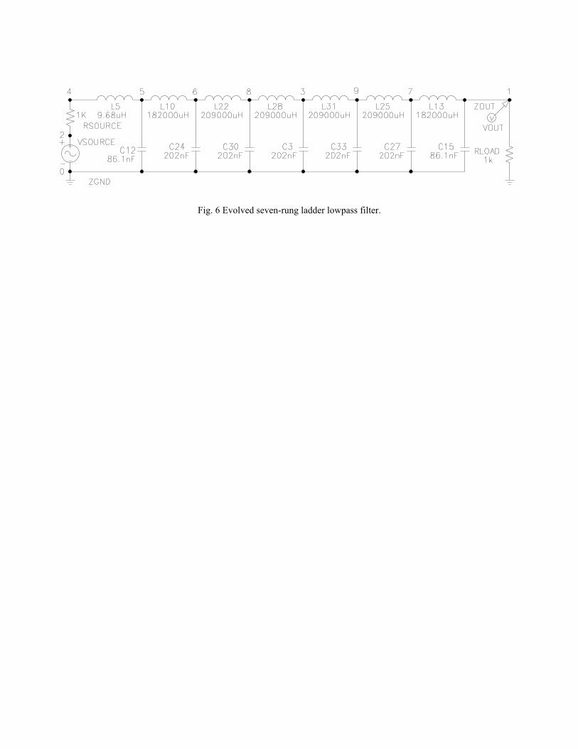
Fig. 6 Evolved seven-rung ladder lowpass filter.

Fig. 7 Frequency domain behavior of genetically evolved 7-rung ladder lowpass filter.

Fig. 8 Evolved four-rung ladder highpass filter.

Fig. 9 Frequency domain behavior of evolved four-rung ladder highpass filter.

Fig. 10 Evolved bandpass filter.

Fig. 11 Frequency domain behavior of evolved bandpass filter.

Fig. 12 Evolved frequency-measuring circuit.

Fig. 13 Frequency domain behavior of evolved frequency-measuring circuit.

Fig. 14 Evolved square root circuit.

Fig. 15 Evolved robot controller.

0 1 2 3

-2

-1

0

1

x

y

(0.409, -0.892)

Fig. 16 Evolved time-optimal trajectory to destination point (0.409, –0.892).

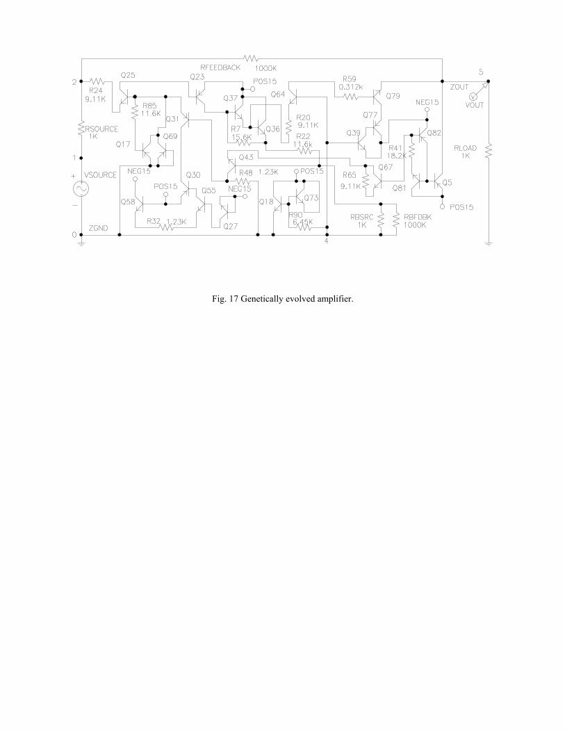
Fig. 17 Genetically evolved amplifier.