automatic induction of classification rules from examples...

Automatic Induction of Classification Rules from Examples Using N-Prism

Max Bramer

Faculty of Technology, University of Portsmouth, Portsmouth, UK [email protected]

www.dis.port.ac.uk/~bramerma

Abstract

One of the key technologies of data mining is the automatic induction of rules from examples, particularly the induction of classification rules. Most work in this field has concentrated on the generation of such rules in the intermediate form of decision trees. An alternative approach is to generate modular classification rules directly from the examples. This paper seeks to establish a revised form of the rule generation algorithm Prism as a credible candidate for use in the automatic induction of classification rules from examples in practical domains where noise may be present and where predicting the classification for previously unseen instances is the primary focus of attention.

1 Introduction In recent years the considerable commercial potential of the sub-field of Machine Learning known as Data Mining has increasingly become recognised. One of the key technologies of data mining is the automatic induction of rules from examples, particularly the induction of classification rules. Many practical questions can be formulated as classification problems, e.g. hospital patients who need an urgent operation, a non-urgent operation or no operation at all, shares which should be sold or bought, those who are likely to respond or not respond to mailshots. Most work in this field has concentrated on the generation of classification rules in the intermediate form of decision trees, although problems with this approach were identified over a decade ago by Cendrowska [1,2]. In work supervised by the present author, Cendrowska proposed a method of generating modular classification rules directly from examples. This paper seeks to bring this work up to date and to establish Prism, in a revised form known as N-Prism, as a credible candidate for use in the automatic induction of classification rules from examples in practical domains where noise may be present and where predicting the classification for previously unseen instances

(rather than finding the most compact representation of a training set) is the primary focus of attention. 2 Automatic Induction of Classification Rules 2.1 Basic Terminology It is assumed that there is a universe of objects, each of which belongs to one of a set of mutually exclusive classes and is described by the values of a collection of its attributes. The attributes may either be categorical, i.e. take one of a set of discrete values, or continuous. Descriptions of a number of objects are held in tabular form in a training set, each row of the table comprising an instance, i.e. the attribute values and the classification corresponding to one object. The aim is to develop classification rules from the data in the training set in order to enable the classification of previously unseen data in a test set to be determined on the basis of its attribute values. As an example, Table 1 below is a fragment of a training set containing the examination results for a set of university students, linking the results for five final-year subjects (coded as SoftEng, ARIN, HCI, CSA and Project), with their degree classifications (First, Second or Third).

SoftEng ARIN HCI CSA Project Class

A B A B B Second A B B B B Second B A A B A Second B A A B B Third A A B B A First B A A B B Third

……… ……… ……… ……… ……… ……… A A B A B First

Table 1. Example Training Set: Degree Classifications

The aim is to derive a set of classification rules from the training set which will enable the degree classification to be correctly estimated for students who are not included in the training set. For the above example some possible rules might be: IF SoftEng = A AND ARIN = A AND Project = A THEN Class = First IF SoftEng = A AND ARIN = A AND CSA = A THEN Class = First IF SoftEng = B AND Project = B THEN Class = Third

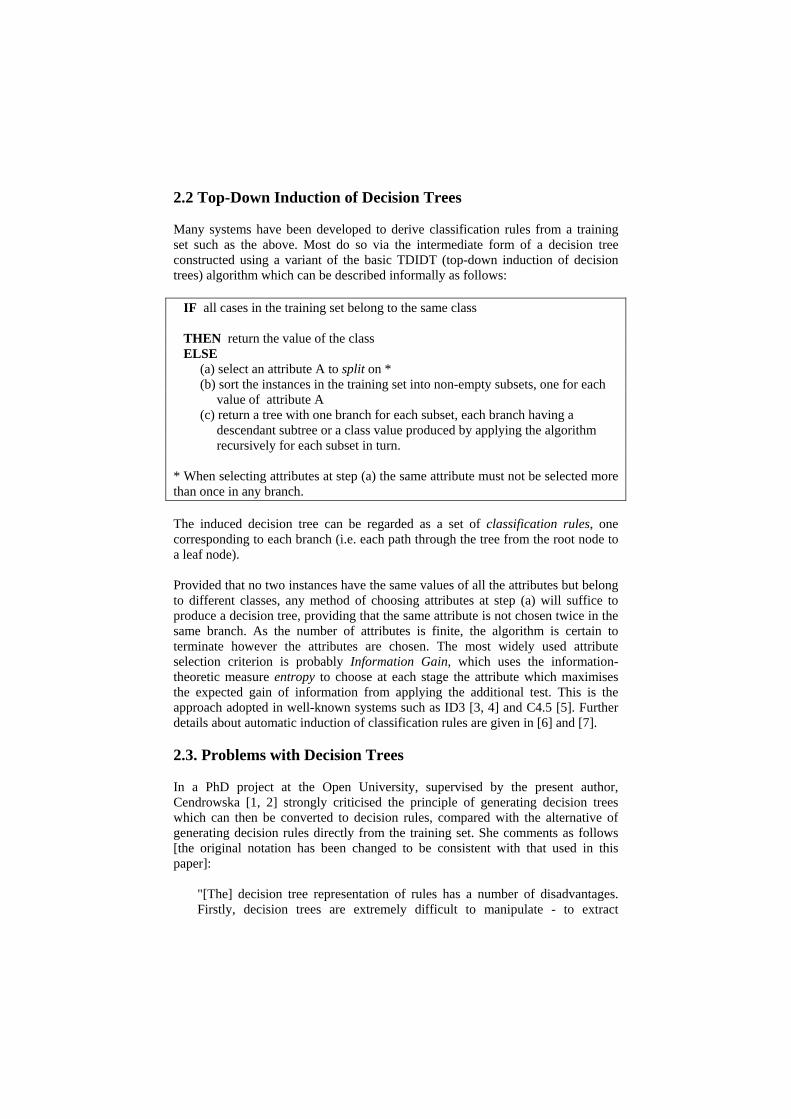
2.2 Top-Down Induction of Decision Trees Many systems have been developed to derive classification rules from a training set such as the above. Most do so via the intermediate form of a decision tree constructed using a variant of the basic TDIDT (top-down induction of decision trees) algorithm which can be described informally as follows: IF all cases in the training set belong to the same class THEN return the value of the class ELSE (a) select an attribute A to split on * (b) sort the instances in the training set into non-empty subsets, one for each value of attribute A (c) return a tree with one branch for each subset, each branch having a descendant subtree or a class value produced by applying the algorithm recursively for each subset in turn. * When selecting attributes at step (a) the same attribute must not be selected more than once in any branch. The induced decision tree can be regarded as a set of classification rules, one corresponding to each branch (i.e. each path through the tree from the root node to a leaf node). Provided that no two instances have the same values of all the attributes but belong to different classes, any method of choosing attributes at step (a) will suffice to produce a decision tree, providing that the same attribute is not chosen twice in the same branch. As the number of attributes is finite, the algorithm is certain to terminate however the attributes are chosen. The most widely used attribute selection criterion is probably Information Gain, which uses the information-theoretic measure entropy to choose at each stage the attribute which maximises the expected gain of information from applying the additional test. This is the approach adopted in well-known systems such as ID3 [3, 4] and C4.5 [5]. Further details about automatic induction of classification rules are given in [6] and [7]. 2.3. Problems with Decision Trees In a PhD project at the Open University, supervised by the present author, Cendrowska [1, 2] strongly criticised the principle of generating decision trees which can then be converted to decision rules, compared with the alternative of generating decision rules directly from the training set. She comments as follows [the original notation has been changed to be consistent with that used in this paper]:

"[The] decision tree representation of rules has a number of disadvantages. Firstly, decision trees are extremely difficult to manipulate - to extract

information about any single classification it is necessary to examine the complete tree, a problem which is only partially resolved by trivially converting the tree into a set of individual rules, as the amount of information contained in some of these will often be more than can easily be assimilated. More importantly, there are rules that cannot easily be represented by trees.

Consider, for example, the following rule set:

Rule 1: IF a = 1 AND b = 1 THEN Class = 1 Rule 2: IF c = 1 AND d = 1 THEN Class =1 Suppose that Rules 1 and 2 cover all instances of Class 1 and all other instances are of Class 2. These two rules cannot be represented by a single decision tree as the root node of the tree must split on a single attribute, and there is no attribute which is common to both rules. The simplest decision tree representation of the set of instances covered by these rules would necessarily add an extra term to one of the rules, which in turn would require at least one extra rule to cover instances excluded by the addition of that extra term. The complexity of the tree would depend on the number of possible values of the attributes selected for partitioning. For example, let the four attributes a, b, c and d each have three possible values 1, 2 and 3, and let attribute a be selected for partitioning at the root node. The simplest decision tree representation of Rules 1 and 2 is shown [below].

[NOTE: In the figure, notation such as a1 is used to denote that the value of attribute a is 1 and 1 to denote that the class value is 1] The paths relating to Class 1 can be listed as follows:

IF a = 1 AND b = 1 THEN Class = 1 IF a = 1 AND b = 2 AND c = 1 AND d = 1 THEN Class = 1 IF a = 1 AND b = 3 AND c = 1 AND d = 1 THEN Class = 1 IF a = 2 AND c = 1 AND d = 1 THEN Class = 1 IF a = 3 AND c = 1 AND d = 1 THEN Class = 1

Clearly, the consequence of forcing a simple rule set into a decision tree representation is that the individual rules, when extracted from the tree, are often too specific (i.e. they reference attributes which are irrelevant). This makes them highly unsuitable for use in many domains."

The phenomenon of unnecessarily large and confusing decision trees described by Cendrowska is far from being merely a rare hypothetical possibility. It will occur whenever there are two (underlying) rules with no attribute in common, a situation that is likely to occur frequently in practice. All the rules corresponding to the branches of a decision tree must begin in the same way, i.e. with a test on the value of the attribute selected at the top level. This effect will inevitably lead to the introduction of terms in rules (branches) which are unnecessary except for the sole purpose of enabling a tree structure to be constructed. Considerable practical problems can arise when the value of the attribute which all the derived rules have in common is unknown at problem-solving time or can only be obtained by means of a test that carries an unusually high cost or risk to health. Systems which generate classification rules e.g. C4.5Rule [5] generally do so by post-pruning, i.e. first generating a classification tree, converting this to a set of equivalent classification rules (one rule per branch of the tree) and then generalising the rules by removing redundant terms. Although reasonably successful this seems an unnecessarily indirect way of generating a set of rules. 2.4 The Prism Algorithm The approach adopted by Cendrowska in her Prism system was to induce classification rules directly from the training set, by selecting a combination of attribute-value pairs to maximise the probability of each target outcome class in turn. In its basic form, the Prism algorithm for induction of classification rules is as follows, assuming that there are n (>1) possible classes: For each class i from 1 to n inclusive: (1) Calculate the probability that class = i for each attribute-value pair (2) Select the attribute-value pair with the maximum probability and create a subset of the training set comprising all instances with the selected combination (for all classes) (3) Repeat 1 and 2 for this subset until it contains only instances of class i. The induced rule is then the conjunction of all the attribute-value pairs selected in creating this subset (4) Remove all instances covered by this rule from the training set Repeat 1-4 until all instances of class i have been removed

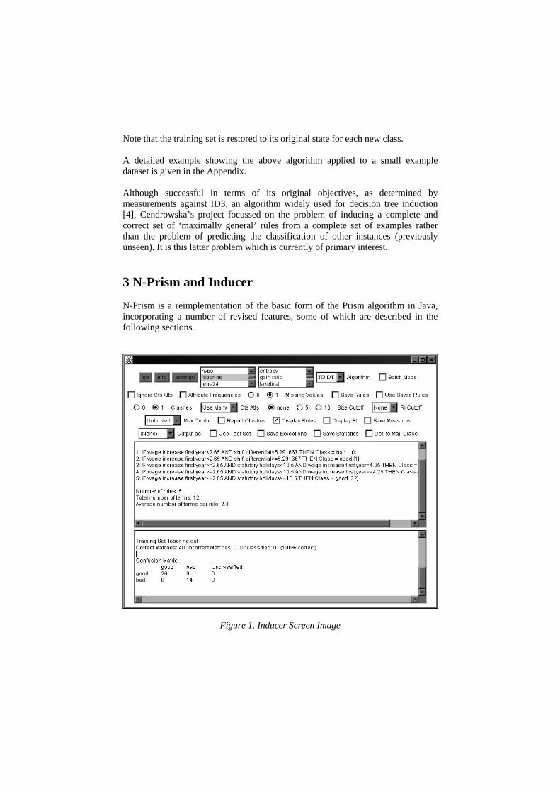
Note that the training set is restored to its original state for each new class. A detailed example showing the above algorithm applied to a small example dataset is given in the Appendix. Although successful in terms of its original objectives, as determined by measurements against ID3, an algorithm widely used for decision tree induction [4], Cendrowska’s project focussed on the problem of inducing a complete and correct set of ‘maximally general’ rules from a complete set of examples rather than the problem of predicting the classification of other instances (previously unseen). It is this latter problem which is currently of primary interest. 3 N-Prism and Inducer N-Prism is a reimplementation of the basic form of the Prism algorithm in Java, incorporating a number of revised features, some of which are described in the following sections.

Figure 1. Inducer Screen Image

The algorithm is implemented in Java version 1.1 as part of the Inducer classification tree and classification rule induction package [8]. The package is available both as a standalone application and as an applet. Inducer also incorporates the TDIDT algorithm with the entropy attribute selection criterion (as well as a range of alternative criteria). Figure 1 shows a screen image of Inducer running the ‘labor negotiations’ dataset from the UCI repository [9]. The package, which was originally developed for teaching purposes, includes a wide range of features to aid the user, including facilities to save rule sets and other information, to apply a variety of cut-offs during tree/rule generation and to adopt different strategies for handling missing data values. In the following sections a number of experiments are described which compare the two principal approaches to classification rule generation implemented in Inducer, i.e. TDIDT with entropy as the attribute selection criterion and Prism in its revised form as N-Prism. The algorithms will generally be referred to simply as TDIDT and Prism where there is no likelihood of confusion arising. Classification trees generated by TDIDT are treated throughout as equivalent to collections of rules, one corresponding to each branch of the tree. The approach adopted here, i.e. comparing two algorithms on a common platform (Inducer) is preferred in the interest of fair comparison to the near-traditional one of making comparison with Quinlan’s well-known program C4.5. The latter contains many additional features developed over a period of years that might potentially be applied to a wide range of other tree/rule generation algorithms as well as the ones included, and therefore might make a fair comparison of basic algorithms difficult to achieve. 4 Rule Set Complexity The complexity of a rule set can be measured in terms of (at least) three parameters:

(a) the number of rules (b) the average number of terms per rule (c) the total number of terms in all rules combined the third value being simply the product of the first two. To compare TDIDT and N-Prism against these three criteria, classification rules were generated using both algorithms for eight selected datasets (training sets). The datasets used are summarised in Table 2. The contact_lenses dataset is a reconstruction of data given in [2]. The chess dataset is a reconstruction of chess endgame data used for experiments described in [10]. The other six datasets have been taken from the well-known UCI repository

of machine learning datasets [9], which is widely used for experiments of this kind. Where necessary, they have been converted to the data format used by Inducer. Further information about the datasets used here and in subsequent experiments is generally provided with the datasets themselves in the UCI repository.

Dataset Description Number of Classes

Number of Attributes

No. of Instances *

agaricus_ lepiota +

Mushroom Records 2 22 5000 (74)

chess Chess Endgame 2 7 647 contact_ lenses

Contact Lenses 3 5 108

genetics Gene Sequences 19 35 3190 monk1 Monk's Problem 1 2 6 124 monk2 Monk's Problem 2 2 6 169 monk3 Monk's Problem 3 2 6 122 soybean Soybean Disease Diagnosis 19 35 683 (121)

Table 2. Datasets used in Rule Set Complexity Experiment

* Figures in parentheses denote the number of instances with missing values included in the previous value. Only non-zero values are shown. Missing values can be handled in a variety of ways. For the purposes of the experiments described in this paper, missing values of an attribute have been replaced by the most commonly occurring value of that attribute in every case. + Only the first 5000 instances in the dataset were used. The table shows the number of attributes used for classification in each of the given datasets. The principal criterion for selecting the datasets was that all the attributes should be categorical, i.e. have a finite number of discrete values. In its present implementation, N-Prism does not accept continuous attributes. In practice this limitation can be overcome if necessary by prior discretization of any continuous attributes using an algorithm such as ChiMerge [11]. A version of N-Prism that includes the processing of continuous attributes is currently under development. 4.1 Experimental Results Table 3 summarises the number of rules, the average number of terms per rule and the total number of terms for all rules combined for both algorithms for each of the eight datasets.

The results are displayed graphically in Figures 2, 3 and 4. In the first two, the number of rules and terms generated by Prism for each dataset have been expressed as a percentage of the figure for TDIDT (given as 100 in each case).

Number of Rules Av. No. of Terms

Total No. of Terms

No. of Instances

TDIDT Prism TDIDT Prism TDIDT Prism agaricus_ lepiota

5000 17 22 2.18 1.23 37 27

chess 647 20 15 5.25 3.20 105 48 contact_ lenses

108 16 15 3.88 3.27 62 49

genetics 3190 389 244 5.71 3.95 2221 963 monk1 124 46 25 4.04 3.00 186 75 monk2 169 87 73 4.74 4.00 412 292 monk3 122 28 26 3.36 2.81 94 73 soybean 683 109 107 5.45 3.57 594 382

Table 3. Comparison of Rule Set Complexity: TDIDT v Prism

R u le s G e n e ra te d

02 04 06 08 0

1 0 01 2 01 4 0

agari

cus_

lepiot

ach

ess

conta

ct_len

ses

gene

tics

monk1

monk2

monk3

soyb

ean

D a ta s e t

Rul

es (a

s %

of T

DID

T)

T D ID TP rism

Figure 2. Comparison of Rule Set Complexity: Rules Generated

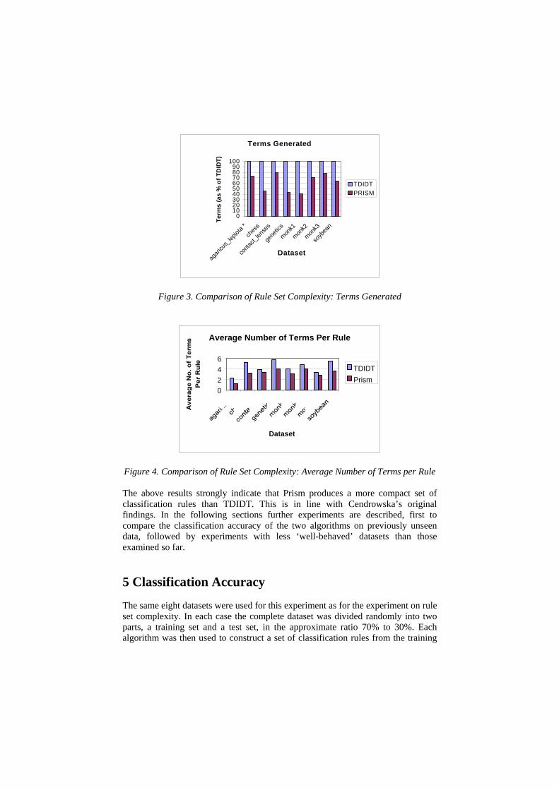
With the (partial) exception of agaricus_lepiota, the results uniformly show that Prism produces fewer rules than TDIDT and that on average each rule includes fewer terms. The combined effect of these results can be a very substantial reduction in the total number of terms generated for all rules combined (down from 2221 to 963 in the case of genetics).

Terms Generated

0102030405060708090

100

agari

cus_

lepiot

a *ch

ess

conta

ct_len

ses

gene

tics

monk1

monk2

monk3

soyb

ean

Dataset

Term

s (a

s %

of T

DID

T)

TDIDTPRISM

Figure 3. Comparison of Rule Set Complexity: Terms Generated

Average Number of Terms Per Rule

0246

Dataset

TDIDTPrism

Figure 4. Comparison of Rule Set Complexity: Average Number of Terms per Rule The above results strongly indicate that Prism produces a more compact set of classification rules than TDIDT. This is in line with Cendrowska’s original findings. In the following sections further experiments are described, first to compare the classification accuracy of the two algorithms on previously unseen data, followed by experiments with less ‘well-behaved’ datasets than those examined so far. 5 Classification Accuracy The same eight datasets were used for this experiment as for the experiment on rule set complexity. In each case the complete dataset was divided randomly into two parts, a training set and a test set, in the approximate ratio 70% to 30%. Each algorithm was then used to construct a set of classification rules from the training

set. The rules were then used to classify the instances in the previously unseen test set. 5.1 Experimental Results Table 4 below summarises the results. The numbers of unseen instances correctly classified by the two algorithms are similar, with a small advantage to TDIDT. The number of incorrectly classified instances is generally smaller in the case of Prism, with a particularly substantial improvement over TDIDT in the case of the genetics dataset.

Correct Incorrect Unclassified

No. of Instances

in Test Set TDIDT Prism TDIDT Prism TDIDT Prism agaricus_ lepiota

1478 1474 1474 1 1 3 3

chess 182 181 178 1 2 0 2 contact_ lenses

33 30 28 3 3 0 2

genetics 950 839 825 90 58 21 67 monk1 36 26 25 9 8 1 3 monk2 52 22 27 28 24 2 1 monk3 36 33 28 3 5 0 3 soybean 204 174 169 22 20 8 15

Table 4. Comparison of Classification Accuracy: TDIDT v. Prism

The main difference between the two algorithms is that Prism generally produces more unclassified instances than TDIDT does. In most cases this corresponds principally to a reduction in the number of misclassified instances. This result is in line with those obtained from other datasets (not reported here). In some task domains, there may be no significant difference between wrongly classified and unclassified instances. In others, it may be of crucial importance to avoid classification errors wherever possible, in which case using Prism would seem to be preferable to using TDIDT. In some domains, unclassified instances may not be acceptable or the principal objective may be to maximise the number of correct classifications. In this case, a method is needed to assign unclassified instances to one of the available categories. There are several ways in which this may be done. A simple technique, which is implemented in Inducer for both TDIDT and Prism, is to assign any unclassified instances in the test set to the largest category in the

training set. Table 5 shows the effect of adjusting the results in Table 4 by assigning unclassified instances to the majority class in each case.

Correct Incorrect No. of Instances

in Test Set TDIDT Prism TDIDT Prism

agaricus_ lepiota

1478 1477 1477 1 1

chess 182 181 180 1 2 contact_ lenses

33 30 29 3 4

genetics 950 849 847 101 103 monk1 36 27 28 9 8 monk2 52 24 28 28 24 monk3 36 33 30 3 6 soybean 204 175 173 29 31

Table 5. Comparison of Classification Accuracy:

Unclassified Assigned to Majority Class With this change the results for TDIDT and Prism are virtually identical, although marginally in favour of TDIDT. More sophisticated methods of dealing with unclassified instances might well swing the balance in favour of Prism. 6 Dealing with Clashes Clashes occur during the classification tree/rule generation process whenever an algorithm is presented with a subset of the training set which contains instances with more than one classification, but which cannot be broken down further. Such a subset is known as a ‘clash set’. The principal cause of clashes is the presence of inconsistent data in the training set, where two or more instances have the same attribute values but different classifications. In such cases, a situation will inevitably occur during tree/rule generation where a subset with mixed classifications is reached, with no further attributes available for selection. The simplest way to deal with clashes is to treat all the instances in the clash set as if they belong to the class of the majority of them and generate a rule (or branch of a classification tree) accordingly. This ‘assign all to majority class’ method is the default method used in Inducer. In its original form Prism had no provision for dealing with clashes. This is in line with the aim of finding compact representations of a complete training set (i.e. a

training set containing all possible combinations of attribute values). However, for practical applications it is imperative to be able to handle clashes. Step (3) of the basic Prism algorithm states: ‘Repeat 1 and 2 for this subset until it contains only instances of class i’. To this needs to be added ‘or a subset is reached which contains instances of more than one class, although all the attributes have already been selected in creating the subset’. The simple approach of assigning all instances in the subset to the majority class does not fit directly into the Prism framework. A number of approaches to doing so have been investigated, the most effective of which would appear to be as follows. If a clash occurs while generating the rules for class i: (a) Determine the majority class for the subset of instances in the clash set. (b) If this majority class is class i, then complete the induced rule for classification

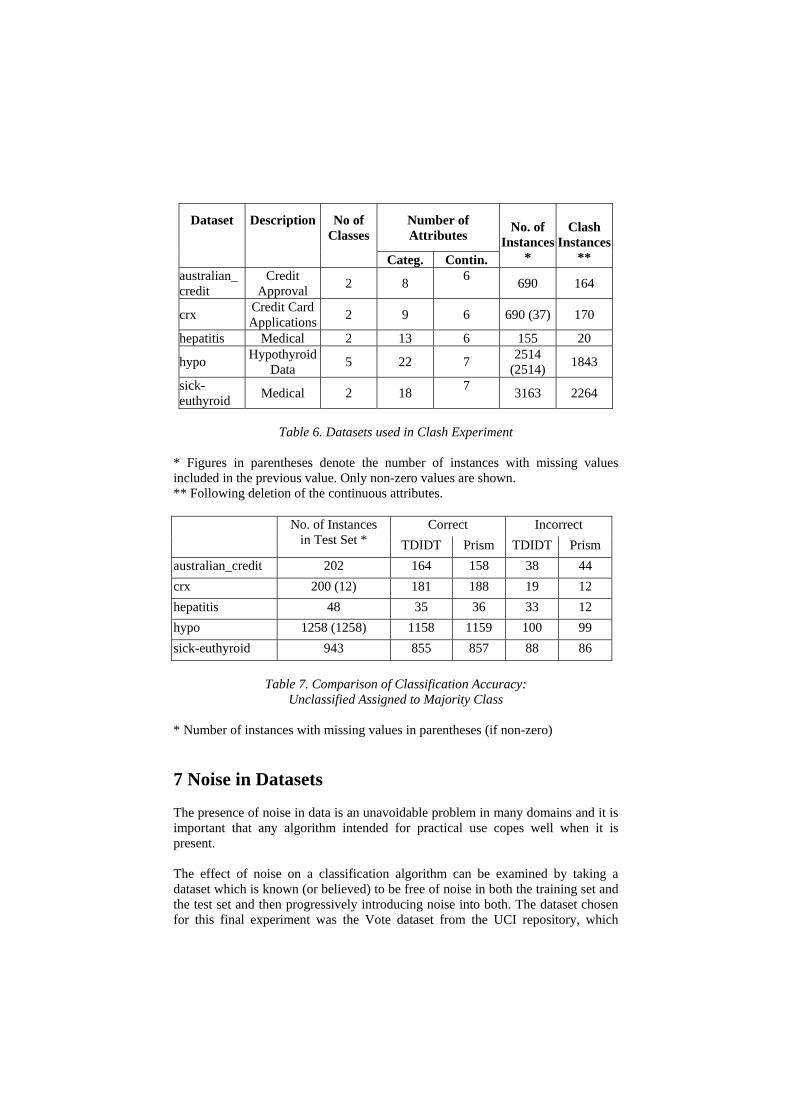
i. If not, discard the rule. 6.1 Clashes in Training Sets The next experiment is a comparison between TDIDT and Prism in the case of datasets where there is a substantial total number of ‘clash instances’. To generate such datasets, five standard datasets were selected from the UCI repository, each with both categorical and continuous attributes. In each case the continuous attributes were effectively discarded, using the ‘ignore continuous attributes’ facility of Inducer. This results in training sets with a high level of inconsistency, from which a significant number of misclassifications of unseen test data would be expected. Table 6 summarises the five datasets used in this experiment. The comparative classification accuracy of the two algorithms is summarised in Table 7, with unclassified instances assigned to the majority class as before. (In the case of TDIDT, clashes encountered during tree generation are handled by the default method described previously.) Although the two algorithms again produce very similar results, in this case Prism outperforms TDIDT for four datasets out of the five tested.

Number of Attributes

Dataset

Description

No of Classes

Categ. Contin.

No. of

Instances *

Clash

Instances **

australian_ credit

Credit Approval 2 8 6 690 164

crx Credit Card Applications 2 9 6 690 (37) 170

hepatitis Medical 2 13 6 155 20

hypo Hypothyroid Data 5 22 7 2514

(2514) 1843

sick-euthyroid Medical 2 18 7 3163 2264

Table 6. Datasets used in Clash Experiment

* Figures in parentheses denote the number of instances with missing values included in the previous value. Only non-zero values are shown. ** Following deletion of the continuous attributes.

Correct Incorrect No. of Instances in Test Set * TDIDT Prism TDIDT Prism

australian_credit 202 164 158 38 44 crx 200 (12) 181 188 19 12 hepatitis 48 35 36 33 12 hypo 1258 (1258) 1158 1159 100 99 sick-euthyroid 943 855 857 88 86

Table 7. Comparison of Classification Accuracy: Unclassified Assigned to Majority Class

* Number of instances with missing values in parentheses (if non-zero) 7 Noise in Datasets The presence of noise in data is an unavoidable problem in many domains and it is important that any algorithm intended for practical use copes well when it is present. The effect of noise on a classification algorithm can be examined by taking a dataset which is known (or believed) to be free of noise in both the training set and the test set and then progressively introducing noise into both. The dataset chosen for this final experiment was the Vote dataset from the UCI repository, which

contains information taken from the 1984 United States congressional voting records. The dataset has 16 attributes (all categorical), 2 classes (Republican and Democrat), with 300 instances in the training set and 135 instances in the test set. As a preliminary to the experiment, a number of versions of both the training set and the test set were generated by introducing noise into the values of all the attributes (including the classification). If the noise level were 20% say, then for each instance in the training or test set every attribute (including the classification) was randomly assigned either a noise value or its own original value on a random basis in proportion 20% to 80%. A ‘noise value’ here denotes any of the valid values for the attribute (or classification), including its original value, chosen with equal probability.

Vote Dataset: Number of Rules Generated

0

50

100

150

0 10 20 30 50 70

% Noise in Training Set

TDIDT Rules Prism Rules

Figure 5. Number of Rules Generated for Varying Levels of Noise in the ‘Vote’ Training Set

Vote Dataset: Number of Terms Generated

0200400600800

0 10 20 30 50 70

% Noise in Training Set

TDIDT TermsPrism Terms

Figure 6. Number of Terms Generated for Varying Levels of Noise in the ‘Vote’ Training Set

For each of a range of levels of noise in the training set (0%, 10%, 20%, 30%, 50% and 70%) a set of classification rules was generated for each algorithm and then used to classify different versions of the test data with noise levels from 0%, 10%, 20% up to 80%. The results of the experiments are summarised in Figures 5-7.

From Figures 5 and 6 it can be seen that TDIDT almost invariably produced more rules and more total terms compared with Prism. As the level of noise in the training set increases, Prism’s advantage also increases until with 70% noise in the training set, the number of rules and terms produced by TDIDT are as much as 55% and 113% greater respectively than those produced by Prism (133 v 86 rules, 649 v 304 terms).

Vote Dataset: 0% Noise in Training Set

0

50

100

150

0 10 20 30 40 50 60 70 80

% Noise in Test Set

Cor

rect

Cla

ssifi

catio

ns

TDIDTPrism


0

50

100

150

0 10 20 30 40 50 60 70 80

% Noise in Test Set

Cor

rect

Cla

ssifi

catio

ns

TDIDTPrism


020406080

100120

0 10 20 30 40 50 60 70 80

% Noise in Test Set

Cor

rect

Cla

ssifi

catio

ns

TDIDTPrism


0

50

100

150

0 10 20 30 40 50 60 70 80

% Noise in Test Set

Cor

rect

Cla

ssifi

catio

ns

TDIDTPrism


020406080

100120

0 10 20 30 40 50 60 70 80

% Noise in Test Set

Cor

rect

Cla

ssifi

catio

ns

TDIDTPrism


020406080

100120

0 10 20 30 40 50 60 70 80

% Noise in Test Set

Cor

rect

Cla

ssifi

catio

ns

TDIDTPrism

Figure 7. Effects of Introducing Noise into the ‘Vote’ Training and Test Sets Figure 7 shows the comparative levels of classification accuracy of the two algorithms for varying levels of noise in the training set. Again Prism outperforms TDIDT in almost all the trials, the advantage increasing as the level of noise increases.

8 Conclusions The experiments presented here suggest that the Prism algorithm for generating modular rules gives classification rules which are at least as good as those obtained from the widely used TDIDT algorithm. There are generally fewer rules with fewer terms per rule, which is likely to aid their comprehensibility to domain experts and users. This result would seem to apply even more strongly when there is noise in the training set. As far as classification accuracy on unseen test data is concerned, there appears to be little to choose between the two algorithms for ‘normal’ (noise-free) datasets, including ones with a significant proportion of clash instances in the training set. The main difference is that Prism generally has a preference for leaving a test instance as ‘unclassified’ rather than giving it a wrong classification. In some domains this may be an important feature. When it is not, a simple strategy such as assigning unclassified instances to the majority class would seem to suffice. When noise is present, Prism would seem to give consistently better classification accuracy than TDIDT, even when there is a high level of noise in the training set. In view of the likelihood of most ‘real world’ datasets containing noise, possibly in a high proportion, these results strongly support the value of using the Prism modular rule approach over the decision trees produced by the TDIDT algorithm. The reasons why Prism should be more tolerant to noise than TDIDT are not entirely clear, but may be related to the presence of fewer terms per rule in most cases. The computational effort involved in generating rules using Prism, at least in its standard form, is greater than for TDIDT. However, Prism would seem to have considerable potential for efficiency improvement by parallelisation. Future investigations will use the Inducer framework to compare Prism, in its revised form as N-Prism, with other less widely used algorithms such as ITRULE [12]. References 1. Cendrowska, J. PRISM: an Algorithm for Inducing Modular Rules. International Journal

of Man-Machine Studies, 1987; 27: 349-370

2. Cendrowska, J. Knowledge Acquisition for Expert Systems: Inducing Modular Rules from Examples. PhD Thesis, The Open University, 1990

3. Quinlan, J.R. Learning Efficient Classification Procedures and their Application to Chess Endgames. In: Michalski, R.S., Carbonell, J.G. and Mitchell, T.M. (eds.), Machine Learning: An Artificial Intelligence Approach. Tioga Publishing Company, 1983

4. Quinlan, J.R. Induction of Decision Trees. Machine Learning, 1986; 1: 81-106 5. Quinlan, J. R. C4.5: Programs for Machine Learning. Morgan Kaufmann, 1993 6. Bramer, M. A. Rule Induction in Data Mining: Concepts and Pitfalls (Part 1). Data

Warehouse Report. Summer 1997; 10: 11-17

7. Bramer, M. A. Rule Induction in Data Mining: Concepts and Pitfalls (Part 2). Data Warehouse Report. Autumn 1997; 11: 22-27

8. Bramer, M. A. The Inducer User Guide and Reference Manual. Technical Report: University of Portsmouth, Faculty of Technology, 1999

9. Blake, C.L. and Merz, C.J. UCI Repository of Machine Learning Databases [http://www.ics.uci.edu/~mlearn/MLRepository.html]. Irvine, CA: University of California, Department of Information and Computer Science, 1998

10. Quinlan, J.R. Discovering Rules by Induction from Large Collections of Examples. In: Michie, D. (ed.), Expert Systems in the Micro-electronic Age. Edinburgh University Press, 1979, pp 168-201

11. Kerber, R. ChiMerge: Discretization of Numeric Attributes. In: Proceedings of the 10th National Conference on Artificial Intelligence. AAAI, 1992, pp 123-128

12. Smyth, P. and Goodman, R.M. Rule Induction Using Information Theory. In: Piatetsky-Shapiro, G. and Frawley, W.J. (eds.), Knowledge Discovery in Databases. AAAI Press, 1991, pp 159-176

13. McSherry, D. Strategic Induction of Decision Trees. In: Miles, R., Moulton, M. and Bramer, M. (eds.), Research and Development in Expert Systems XV. Springer-Verlag, 1999, pp 15-26

Appendix. Prism: A Worked Example The following example shows in detail the operation of the basic Prism algorithm when applied to the training set lens24, which has 24 instances. This dataset was introduced by Cendrowska [1,2] and has been widely used subsequently (see for example [13]). It is a subset of Cendrowska’s 108-instance contact_lenses dataset referred to in Table 2. The attributes age, specRx, astig and tears correspond to the age of the patient, the spectacle prescription, whether or not the patient is astigmatic and his or her tear production rate, respectively. The three possible classifications are that the patient should be fitted with (1) hard contact lenses, (2) soft contact lenses or (3) is not suitable for wearing contact lenses. In this example, Prism is used to generate the classification rules corresponding to class 1 only. It does so by repeatedly making use of the probability of attribute-value pairs.

age specRx astig tears class 1 1 1 1 3 1 1 1 2 2 1 1 2 1 3 1 1 2 2 1 1 2 1 1 3 1 2 1 2 2 1 2 2 1 3 1 2 2 2 1 2 1 1 1 3 2 1 1 2 2 2 1 2 1 3 2 1 2 2 1 2 2 1 1 3 2 2 1 2 2 2 2 2 1 3 2 2 2 2 3 3 1 1 1 3 3 1 1 2 3 3 1 2 1 3 3 1 2 2 1 3 2 1 1 3 3 2 1 2 2 3 2 2 1 3 3 2 2 2 3

Table 8. The lens24 Training Set

Class 1: First Rule The table below shows the probability of each attribute-value pair occurring for the whole training set (24 instances).

Attribute-value pair Frequency for class = 1

Total Frequency (24 instances)

Probability

age = 1 2 8 0.25 age = 2 1 8 0.125 age = 3 1 8 0.125 specRx = 1 3 12 0.25 specRx = 2 1 12 0.083 astig = 1 0 12 0 astig = 2 4 12 0.33 tears = 1 0 12 0 tears = 2 4 12 0.33

The attribute-value pairs that maximise the probability of Class 1 are astig = 2 and tears = 2. Choose astig = 2 arbitrarily. The (incomplete) rule induced so far is: IF astig = 2 THEN class = ?

The subset of the training set covered by this rule is:

age specRx astig tears class 1 1 2 1 3 1 1 2 2 1 1 2 2 1 3 1 2 2 2 1 2 1 2 1 3 2 1 2 2 1 2 2 2 1 3 2 2 2 2 3 3 1 2 1 3 3 1 2 2 1 3 2 2 1 3 3 2 2 2 3

The next table shows the probability of each attribute-value pair (not involving attribute astig) occurring for this subset



Probability

age = 1 2 4 0.5 age = 2 1 4 0.25 age = 3 1 4 0.25 specRx = 1 3 6 0.5 specRx = 2 1 6 0.17 tears = 1 0 6 0 tears = 2 4 6 0.67

The maximum probability occurs when tears = 2 Rule induced so far: IF astig = 2 and tears = 2 THEN class = ? The subset of the training set covered by this rule is now

age specRx astig tears class 1 1 2 2 1 1 2 2 2 1 2 1 2 2 1 2 2 2 2 3 3 1 2 2 1 3 2 2 2 3

The next table shows the probability of each attribute-value pair occurring for this subset



Probability

age = 1 2 2 1.0 age = 2 1 2 0.5 age = 3 1 2 0.5 specRx = 1 3 3 1.0 specRx = 2 1 3 0.33

The maximum probability occurs when age = 1 or specRx = 1. Choose (arbitrarily) age = 1 Rule induced so far: IF astig = 2 and tears = 2 and age = 1 THEN Class = ? The subset of the training set covered by this rule is:

age specRx astig tears class 1 1 2 2 1 1 2 2 2 1

This subset contains only instances of class 1. The final induced rule is therefore IF astig = 2 and tears = 2 and age = 1 THEN Class = 1 Class 1: Second Rule Removing all instances covered by this rule from the training set gives a new training set (22 instances)

age specRx astig tears class 1 1 1 1 3 1 1 1 2 2 1 1 2 1 3 1 2 1 1 3 1 2 1 2 2 1 2 2 1 3 2 1 1 1 3 2 1 1 2 2 2 1 2 1 3 2 1 2 2 1 2 2 1 1 3 2 2 1 2 2 2 2 2 1 3 2 2 2 2 3 3 1 1 1 3 3 1 1 2 3 3 1 2 1 3 3 1 2 2 1 3 2 1 1 3 3 2 1 2 2 3 2 2 1 3 3 2 2 2 3

The table of frequencies for attribute-value pairs corresponding to class = 1 is now as follows



Probability

age = 1 0 6 0 age = 2 1 8 0.125 age = 3 1 8 0.125 specRx = 1 2 11 0.18 specRx = 2 0 11 0 astig = 1 0 12 0 astig = 2 2 10 0.2 tears = 1 0 12 0 tears = 2 2 10 0.2

The maximum probability occurs when astig = 2 or tears = 2. Choose astig=2 arbitrarily. Rule induced so far: IF astig=2 THEN Class= ? The subset of the training set covered by this rule is:

age specRx astig tears class 1 1 2 1 3 1 2 2 1 3 2 1 2 1 3 2 1 2 2 1 2 2 2 1 3 2 2 2 2 3 3 1 2 1 3 3 1 2 2 1 3 2 2 1 3 3 2 2 2 3

Giving the following frequency table



Probability

age = 1 0 2 0 age = 2 1 4 0.25 age = 3 1 4 0.25 specRx = 1 0 5 0 specRx = 2 2 5 0.4 tears = 1 0 6 0 tears = 2 2 4 0.5

The maximum probability occurs when tears = 2. Rule induced so far: IF astig = 2 and tears = 2 then class = ?

The subset of the training set covered by this rule is:

age specRx astig tears class 2 1 2 2 1 2 2 2 2 3 3 1 2 2 1 3 2 2 2 3

Giving the following frequency table



Probability

age = 1 0 0 age = 2 1 2 0.5 age = 3 1 2 0.5 specRx = 1 2 2 1.0 specRx = 2 0 2 0

The maximum probability occurs when specRx = 1 Rule induced so far: IF astig = 2 and tears = 2 and specRx = 1 THEN class = ? The subset of the training set covered by this rule is:

age specRx astig tears class 2 1 2 2 1 3 1 2 2 1

This subset contains only instances of class 1. So the final induced rule is: IF astig = 2 and tears = 2 and specRx = 1 THEN class = 1 Removing all instances covered by this rule from the training set (i.e. the version with 22 instances) gives a training set of 20 instances from which all instances of class 1 have now been removed. So the Prism algorithm terminates (for class 1). The two rules induced by Prism for Class 1 are therefore: IF astig = 2 and tears = 2 and age = 1 THEN class = 1 IF astig = 2 and tears = 2 and specRx = 1 THEN class = 1

automatic induction of classification rules from examples...

Documents