automated recognition of wood used in traditional japanese
TRANSCRIPT

ORIGINAL ARTICLE
Automated recognition of wood used in traditional Japanesesculptures by texture analysis of their low-resolution computedtomography data
Kayoko Kobayashi1 • Masanori Akada2 • Toshiyuki Torigoe3 • Setsuo Imazu2 •
Junji Sugiyama1
Received: 3 June 2015 / Accepted: 4 August 2015 / Published online: 4 September 2015
� The Author(s) 2015. This article is published with open access at Springerlink.com
Abstract The identification of wood species used in the
cultural artifacts is important in terms of their preservation
and inheritance. However, a nondestructive method is
required, and wood samples must be partly cut off in
conventional methods such as microscopy. In this study,
we constructed a novel system for wood identification
using image recognition of X-ray computed tomography
images of eight major species used in Japanese wooden
sculptures. Texture analyses of the computed tomography
images were carried out using the gray-level co-occurrence
matrix, from which 15 textural features were calculated.
The k-nearest-neighbor algorithm combined with cross
validation was applied for classification and evaluation of
the system. Input datasets with a variation in image qual-
ities (resolution, gray level, and image size) were investi-
gated using this novel system, and the accuracy was greater
than 98 % when the input images had a certain quality
level. Although there are still technical problems to be
overcome, progress in the development of automated
identification is extremely encouraging in that such an
approach has the potential to make a valuable contribution
in adding scientific species notion to the artifacts; other-
wise, only the literal documents are available.
Keywords Wood identification � Pattern recognition �Texture analysis � Gray-level co-occurrence matrix �X-ray computer tomography
Introduction
Wood identification has been providing useful information
of the origins of heritages and sometimes provided a new
perspective. Although it requires expertise in wood anat-
omy, the technique has increasingly been used by curators
and archeologists owing to the list of anatomical features
published by the IAWA Comittee [1, 2]. Commonly, wood
samples have to be observed from three orthogonal direc-
tions, namely, the transverse, radial, and tangential direc-
tions, to obtain the appropriate information of their
anatomical features. This method becomes routine after
training and experience, but it is not applicable to culturally
important wood works or artifacts, where only nonde-
structive methods are allowed to be used.
Spectroscopy is one example of a nondestructive and
noninvasive method, and several attempts to identify wood
have been successfully reported [3–5]. The prediction
accuracy can be improved by the quality of the spectral
database, but is not sufficient for the classification of a
wide range of wood species. It is more efficient if the target
species for classification are limited. Another nondestruc-
tive technique is X-ray computed tomography (CT). One
example is the use of synchrotron radiation X-ray micro-
tomography, where the three-dimensional (3D) wood
structure has been reconstructed at a resolution of 0.5 lm[6]. In this technique, wood identification based on the
IAWA list [1, 2] is possible. However, the sample size and
machine time are limited; therefore, the measurement is
limited to selected important materials.
& Kayoko Kobayashi
1 Research Institute for Sustainable Humanosphere, Kyoto
University, Gokasho, Uji, Kyoto 611-0011, Japan
2 Kyushu National Museum, Dazaifu, Fukuoka 818-0118,
Japan
3 Nara National Museum, Nara, Nara 630-8213, Japan
123
J Wood Sci (2015) 61:630–640
DOI 10.1007/s10086-015-1507-6

Kyushu National Museum was the fourth national
museum in Japan, and it is devoted to the scientific
investigation of artwork. Since the installation of a large-
scale X-ray CT instrument, nearly 2000 wooden artifacts
have been inspected. Unfortunately, the images were never
considered as resources for analyzing wood properties.
This is because the resolution of the image was too low to
apply conventional wood identification that relies on the
visual inspection of microscopic anatomical features.
For the last several decades, image recognition tech-
nology, such as an automated face-recognition system and
fingerprint authentication, has been significantly devel-
oped. As a method for the extraction of image information,
which is one of the important processes in image recog-
nition, a texture analysis has been utilized in a variety of
fields such as remote sensing and medical imaging. Several
authors have also reported attempts of the application of
these techniques to wood identification [7–19], which are
particularly active in tropical areas. Tropical timber is an
important biological and economical resource in the
developing world; thus, wood identification is demanded at
trading locations to circulate proper wood in the market as
well as to keep illegally logged timber under observation.
Under such circumstances, an automated wood identifica-
tion system is highly demanded because the development
of human resources is important, but it is not straightfor-
ward to train people to have in-depth anatomical knowl-
edge and experience to cover the large diversity of tropical
hardwood species. Many studies have mostly used optical
micrographs [10, 11, 14, 19] or stereograms [7–9, 12, 13,
15–18], whose resolution was a several micrometers at
worst. Under such conditions, the arrangements of vessels
and axial parenchyma were clearly recorded and used as
image information. Several approaches for the extraction of
image information were tested, such as the segmentation of
specific anatomical features [10, 11], the gray-level co-
occurrence matrix (GLCM) [7–9], Gabor filtering [16],
Gabor filtering followed by the GLCM [12], the Coiflet
discrete wavelet transform [18], the extended higher local
order autocorrelation [15], and local binary patterns [14].
Combinations of multiple extractors were also tested for
further improvement in the systems [13, 17, 19].
Inspired by the above-mentioned development of auto-
mated recognition systems, the computer-aided recognition
of low-resolution CT images recorded at Kyushu National
Museum seemed to have a potential to be uncovered.
Although the resolution of the original CT images does not
allow for visualization of individual anatomical features,
the density gradient and fluctuation that are specific to the
species are certainly recorded.
Therefore, the eight most frequently used wood species
in Japanese sculptures were selected and analyzed in this
study. As for the feature extraction procedure, the most
simple and reputable technique, the GLCM that considers
the spatial gray-level distribution [20], was considered to
be the best as the first choice. The detailed procedures and
the applicability of the automated wood identification
technique will be described.
Methods
Wood samples
Ten types of wood blocks were selected by Mr. Yano
Ken’ichiro at the Tokyo University of the Arts, Institute of
Ancient Art Research, Nara from critical/practical view-
points as a professional sculptor. They are Cinnamomum
camphora (Cc), Cercidiphyllum japonicum (Ce), Cryp-
tomeria japonica* (Cj), Chamaecyparis obtusa* (Co),
Magnolia obovata (Mo), Pawlounia tomentosa (Pt), Tor-
reya nucifera (Tn), and Zelkova serrata (Zs). Species with
asterisk have two variations—one from a plantation forest
(Cj1, Co1) and the other from a natural forest (Cj2, Co2).
X-ray computed tomography
X-ray CT experiments of the wood samples were per-
formed using the large-scale X-ray CT instrument (Y.CT
Modular, YXLON International GmbH, Germany) at the
Kyushu National Museum. Al-filtered X-rays were gener-
ated at 225 kV and 30 mA. A total of 1080 projections
were recorded on a flat-panel detector and reconstructed by
employing the filtered back-projection procedure. The
sample-source distance was set to achieve a voxel resolu-
tion of 0.05 mm.
Initial image dataset
From the reconstructed 3D dataset of the wood blocks,
two-dimensional (2D) images were precisely cropped in
the direction that provides a transverse section using vol-
ume graphics software (VGStudio MAX 2.1, Volume
Graphics GmbH, Germany). The images have dimensions
of 300 pixels 9 300 pixels that correspond to
1.5 cm 9 1.5 cm in actual size and a 256-level gray scale.
Forty images were randomly collected for each wood
block, and a total of 400 images in the TIFF file format
were used as an initial dataset.
Computational approaches
An outline of the analysis procedure is shown in Fig. 1.
From the initial dataset, datasets with a variety of qualities
were created, and each dataset was then input into the
recognition system. The system consists of two steps:
J Wood Sci (2015) 61:630–640 631
123

feature extraction and classification. Statistical processing
of all of the following images was carried out using R
version 3.1.1 [21] and its packages.
Preprocessing images
In addition to the initial dataset, a number of datasets
was created by reductions in the resolution, the number
of gray levels, and the image size. The resolution and
image size, which were originally 0.05 mm and
1.5 cm 9 1.5 cm, respectively, were changed using a
function in the ‘‘biOps’’ package [22]. The resolution
was reduced to 0.1, 0.15, 0.2, and 0.25 mm, and the
image size was reduced to 1 cm 9 1 cm and
0.5 cm 9 0.5 cm. The number of gray levels, which was
initially 256 (=28), was reduced, and images with 2n
(n = 3–7) gray levels were generated. In total, 90 data-
sets with five resolutions, six different numbers of gray
levels, and three image sizes were used for further
analysis.
Feature extraction
The GLCM from an image with 2n gray levels is a matrix
with dimensions of 2n 9 2n. The matrix P(i, j) represents
the probability of occurrence of the pair of gray levels i and
j at a separation distance d. In our study, d was fixed to 1,
and the GLCMs were calculated from four directions,
which are horizontal (‘‘0�’’), vertical (‘‘90�’’), and diagonal
(‘‘45�’’ and ‘‘135�’’). In addition to the four GLCMs, one
new matrix was added, which is the ‘‘average’’ of those of
the four directions.
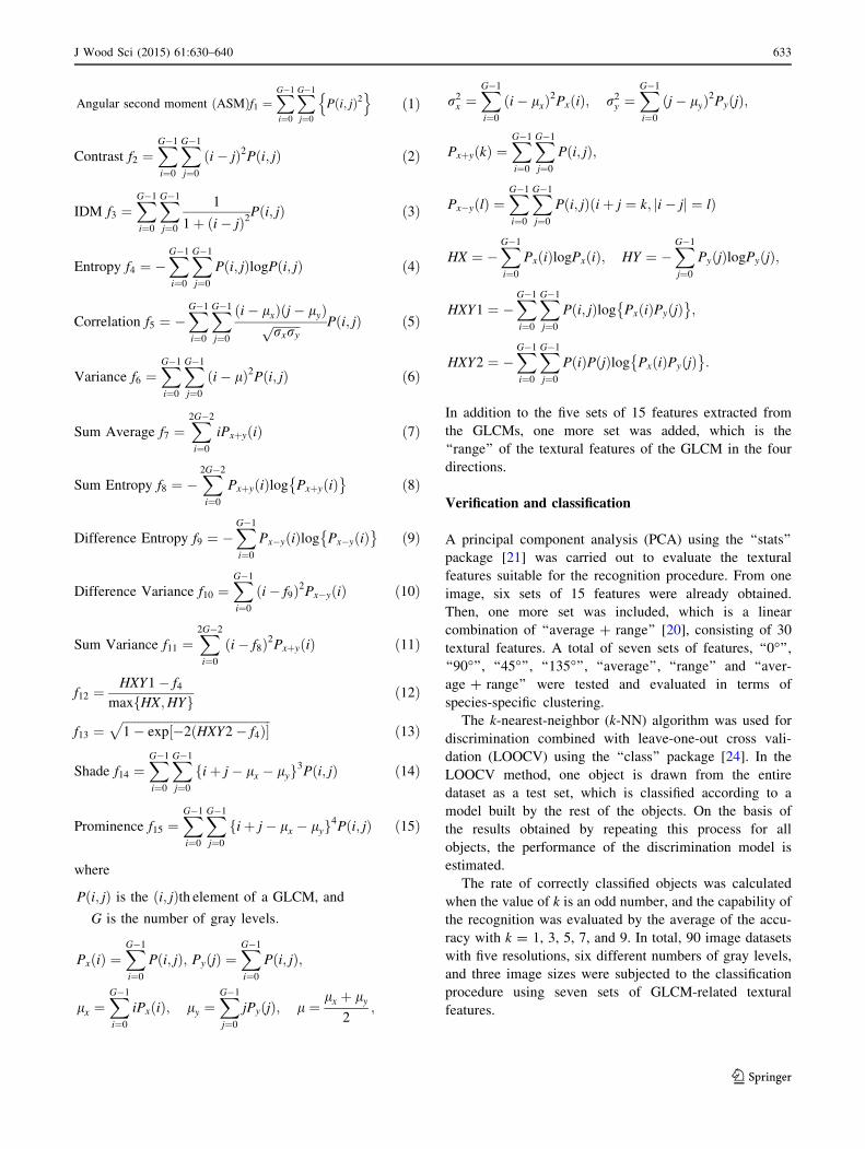
A total of 15 textural features were extracted from each
GLCM, including the 13 textural features proposed by
Haralick et al. [20] and the two textural features added by
Albregtsen [23], which are given as follows:
Classification k-NN algorithm
for 7 sets of textural features ( “0°,” “45°,” “90°,”“135°,” “average,” “range,” “average + range”)
Feature Extraction Construction of GLCMs
for 4 bearing angles ( “0°,” “45°,” “90°,” “135°”) and their “average”
15 Haralick textural featuresfor 5 GLCMs ( “0°,” “45°,” “90°,” “135°,” “average”) and their “range”
Input
Output
Image Processing Resolution reduction
(0.05, 0.1, 0.15, 0.2, 0.25 mm)
Gray-level reduction (256, 128, 64, 32, 16, 8)
Cropping (1.5 × 1.5, 1 × 1, 0.5 × 0.5 cm)
* Bold types indicate the qualities of the initial dataset.
X-ray CT3D dataset(10 wood samples)
2D images of transverse section( 40 images for each wood)
90datasets R e c o g n i t i o n
S y s t e mR e c o g n i t i o n
S y s t e m
400 imagesin initial dataset
Fig. 1 Schematic diagram of
the analysis procedure
632 J Wood Sci (2015) 61:630–640
123
Angular second moment ASMð Þf1 ¼XG�1
i¼0
XG�1
j¼0
P i; jð Þ2n o
ð1Þ
Contrast f2 ¼XG�1
i¼0
XG�1
j¼0
i� jð Þ2P i; jð Þ ð2Þ
IDM f3 ¼XG�1
i¼0
XG�1
j¼0
1
1þ ði� jÞ2Pði; jÞ ð3Þ
Entropy f4 ¼ �XG�1
i¼0
XG�1
j¼0
P i; jð ÞlogP i; jð Þ ð4Þ
Correlation f5 ¼ �XG�1
i¼0
XG�1
j¼0
ði� lxÞðj� lyÞffiffiffiffiffiffiffiffiffirxry
p Pði; jÞ ð5Þ
Variance f6 ¼XG�1
i¼0
XG�1
j¼0
ði� lÞ2P i; jð Þ ð6Þ
Sum Average f7 ¼X2G�2
i¼0
iPxþy ið Þ ð7Þ
Sum Entropy f8 ¼ �X2G�2
i¼0
Pxþy ið Þlog Pxþy ið Þ� �
ð8Þ
Difference Entropy f9 ¼ �XG�1
i¼0
Px�y ið Þlog Px�y ið Þ� �
ð9Þ
Difference Variance f10 ¼XG�1
i¼0
i� f9ð Þ2Px�y ið Þ ð10Þ
Sum Variance f11 ¼X2G�2
i¼0
i� f8ð Þ2Pxþy ið Þ ð11Þ
f12 ¼HXY1� f4
max HX;HYf g ð12Þ
f13 ¼ffiffiffiffiffiffiffiffiffiffiffiffiffiffiffiffiffiffiffiffiffiffiffiffiffiffiffiffiffiffiffiffiffiffiffiffiffiffiffiffiffiffiffiffiffiffiffiffiffi1� exp½�2ðHXY2� f4Þ�
pð13Þ
Shade f14 ¼XG�1
i¼0
XG�1
j¼0
fiþ j� lx � lyg3P i; jð Þ ð14Þ
Prominence f15 ¼XG�1
i¼0
XG�1
j¼0
fiþ j� lx � lyg4P i; jð Þ ð15Þ
where
Pði; jÞ is the ði; jÞth element of a GLCM, and
G is the number of gray levels:
PxðiÞ ¼XG�1
i¼0
Pði; jÞ; PyðjÞ ¼XG�1
i¼0
Pði; jÞ;
lx ¼XG�1
i¼0
iPxðiÞ; ly ¼XG�1
j¼0
jPyðjÞ; l ¼lx þ ly
2;
r2x ¼XG�1
i¼0
ði� lxÞ2PxðiÞ; r2y ¼XG�1
i¼0
ðj� lyÞ2PyðjÞ;
PxþyðkÞ ¼XG�1
i¼0
XG�1
j¼0
Pði; jÞ;
Px�yðlÞ ¼XG�1
i¼0
XG�1
j¼0
Pði; jÞðiþ j ¼ k; ji� jj ¼ lÞ
HX ¼ �XG�1
i¼0
PxðiÞlogPxðiÞ; HY ¼ �XG�1
j¼0
PyðjÞlogPyðjÞ;
HXY1 ¼ �XG�1
i¼0
XG�1
j¼0
Pði; jÞlog PxðiÞPyðjÞ� �
;
HXY2 ¼ �XG�1
i¼0
XG�1
j¼0
PðiÞPðjÞlog PxðiÞPyðjÞ� �
:
In addition to the five sets of 15 features extracted from
the GLCMs, one more set was added, which is the
‘‘range’’ of the textural features of the GLCM in the four
directions.
Verification and classification
A principal component analysis (PCA) using the ‘‘stats’’
package [21] was carried out to evaluate the textural
features suitable for the recognition procedure. From one
image, six sets of 15 features were already obtained.
Then, one more set was included, which is a linear
combination of ‘‘average ? range’’ [20], consisting of 30
textural features. A total of seven sets of features, ‘‘0�’’,‘‘90�’’, ‘‘45�’’, ‘‘135�’’, ‘‘average’’, ‘‘range’’ and ‘‘aver-
age ? range’’ were tested and evaluated in terms of
species-specific clustering.
The k-nearest-neighbor (k-NN) algorithm was used for
discrimination combined with leave-one-out cross vali-
dation (LOOCV) using the ‘‘class’’ package [24]. In the
LOOCV method, one object is drawn from the entire
dataset as a test set, which is classified according to a
model built by the rest of the objects. On the basis of
the results obtained by repeating this process for all
objects, the performance of the discrimination model is
estimated.
The rate of correctly classified objects was calculated
when the value of k is an odd number, and the capability of
the recognition was evaluated by the average of the accu-
racy with k = 1, 3, 5, 7, and 9. In total, 90 image datasets
with five resolutions, six different numbers of gray levels,
and three image sizes were subjected to the classification
procedure using seven sets of GLCM-related textural
features.
J Wood Sci (2015) 61:630–640 633
123

Results and discussion
Extraction of features from CT images
Figure 2 shows the representative CT images of transverse
sections without any image processing, where a darker area
corresponds to an area of lower density. The images were
cropped so that the annual rings are arranged in the vertical
direction, although some images from Cryptomeria
japonica from the plantation forest (Cj1) were difficult to
arrange in this manner because its wood block had smaller
annual rings in diameter. The microscopic anatomical
features were not well observed in these images as
expected, but they obviously showed some differences
among the species. In particular, features related to the
annual rings, such as their widths and the gradient from a
darker area to a lighter area that corresponds to earlywood
to latewood in an annual ring, were readily recognized. The
annual ring boundaries in softwood such as Cj and Co, for
instance, were quite sharp, whereas diffuse-porous hard-
wood such as Ce and Mo exhibited blurred images. In
addition, large pores were also observed as dark dots or
lines in ring-porous hardwoods, Pt and Zs, and diffuse-
porous hardwoods with large vessels, Cc.
These CT images were subsequently converted into
GLCMs, which represent the probabilities of each combi-
nation of gray levels of neighboring pairs occurring in an
image. Figure 3 shows the GLCMs obtained from some of
the images in Fig. 2 after a reduction in the number of gray
levels to 64; thus, the GLCMs consist of 64 columns and 64
rows. Comparing the GLCMs of Zs among the four bearing
angles (Fig. 3a), the elements in the GLCM of ‘‘90�,’’which corresponded to the direction along the annual rings,
were more concentrated along the diagonal than those of
Fig. 2 Typical cross-sectional 2D images from CT datasets obtained
from 10 types of woods, with arrows indicating the directions of the
bearing angles for the construction of GLCMs. Cc, Cinnamomum
camphora; Ce, Cercidiphyllum japonica; Cj1, Cryptomeria japonica
(from a plantation forest); Cj2, Cryptomeria japonica (from a natural
forest); Co1, Chamaecyparis obtusa (from a plantation forest); Co2,
Chamaecyparis obtusa (from a natural forest); Mo, Magnolia
obovata; Pt, Paulownia tomentosa; Tn, Torreya nucifera; and Zs,
Zelkova serrata. The images have a resolution of 0.05 mm, 256 gray
levels, and an actual size of 1.5 cm 9 1.5 cm
634 J Wood Sci (2015) 61:630–640
123

the other directions, indicating that more neighboring
pixels have the same or nearly the same gray level. On the
other hand, the elements were slightly dispersed from the
diagonal in the GLCM of ‘‘0�,’’ which resulted from the
transition of gray levels across the annual rings. The
GLCMs of ‘‘45�’’ and ‘‘135�,’’ consisting of neighboring
pairs in the direction diagonally across the annual rings,
exhibited more dispersed patterns.
The GLCMs of Cj2, Mo, and Zs obtained with the
‘‘average’’ among the four bearing angles are shown in
Fig. 3b. In the GLCM of Cj2, many elements gathered at
the left lower side, but a small quantity of elements also
spread to the right upper side for a wide range (Fig. 3b-1).
This is because the image of Cj2 mainly consists of large
dark areas corresponding to earlywood, but they gradually
transition to small light areas corresponding to latewood.
From the blurred image of Mo, on the other hand, the
GLCM consisted of fewer elements, and they were con-
centrated on the diagonal (Fig. 3b-2). In the GLCM of Zs
(Fig. 3b-3), there are also many elements along the diag-
onal, and some of them are dispersed from the diagonal.
Some neighboring pairs in the image of Zs have large
differences in gray levels due to the large pores.
From the GLCMs obtained from the images, 15 textural
features were calculated. Here, the meanings of the features
are specifically explained using three of them calculated
from the GLCMs shown in Fig. 3b as concrete examples
(Fig. 4). ASM is the sum of the squares of all elements, as
expressed by Eq. 1; thus, a GLCM consisting of fewer
elements makes ASM larger, representing a measure of
homogeneity. Comparing the values of ASM among the
three wood species, the value for Mo was much greater
than those for Co2 and Zs, which is consistent with the
visual appearances of the images. Because contrast, which
becomes larger if there are more elements in the GLCM far
from the diagonal of i = j (Eq. 2), represents the amount of
the local density variation, Co2 and Zs exhibited larger
values. Variance is the degree of variability from the
average of all elements (Eq. 3), resulting in the largest
value for Co2 among the three because the difference in
gray levels is extreme in its image.
Classification and evaluation of the recognition
system
Before classification using the extracted textural features,
they were analyzed by a PCA for testing the clustering of
objects and the dispersion of the textural features in the
feature space. Figure 5 shows examples of the results of the
PCA, which were obtained using the features calculated
from ‘‘average,’’ ‘‘range,’’ and ‘‘average ? range’’ of
images with 64 gray levels. In most cases, the 15 textural
features pointed in diverse directions in the score plot, as
shown in Fig. 5a, indicating that every feature has mean-
ingful information for discrimination. As a result, the
objects were well dispersed and clustered for each class. In
contrast, in some cases shown in Fig. 5b, many textural
features exhibited similar directions, and several clusters
10 20 30 40 50 60
1020
3040
5060
i
j
10 20 30 40 50 60
1020
3040
5060
i
j
10 20 30 40 50 60
1020
3040
5060
i
j
10 20 30 40 50 60
1020
3040
5060
i
j
10 20 30 40 50 60
1020
3040
5060
i
j
a-1
10 20 30 40 50 60
1020
3040
5060
i
j
10 20 30 40 50 60
1020
3040
5060
i
j
a-2
b-1
a-4a-3
b-3b-2
Fig. 3 Gray-level co-occurrence matrices (GLCMs) calculated from
some of the images in Fig. 2 with a reduction of the number of gray
levels to 64. Elements with higher values are indicated by darker
colors. a Comparison of the GLCMs obtained from Zs with different
bearing angles of ‘‘0�’’, ‘‘45�’’, ‘‘90�’’ and ‘‘135�’’. b Comparison of
GLCMs obtained from different wood species: Co2, Mo, and Zs. The
parameter used for the calculation is ‘‘average’’
J Wood Sci (2015) 61:630–640 635
123

for each class overlapped with each other. Using the
combined 30 features of ‘‘average ? range’’ (Fig. 5c), the
objects seemed to be discriminated as well as or better than
the case in which only the 15 features of ‘‘average’’ were
used, even though some of the features pointed in similar
directions.
The k-NN algorithm was adopted for classification, and
the accuracy of the recognition system was estimated by
LOOCV for each value of k. Figure 6 shows the changes in
the accuracy depending on k when using the same dataset
and parameters as in Fig. 5. The accuracy remained almost
constant with the increase in k when ‘‘average’’ and ‘‘av-
erage ? range’’ were used (Fig. 6a, c), whereas it gradu-
ally decreased in the case of ‘‘range’’ (Fig. 6b). This is
because an object is misclassified into the wrong class with
a higher probability with increasing k if there is an object
located between its true cluster and the other ones. These
results were consistent with the PCA analysis, where
0
20
40
60
80
100
variance0
5
10
15
20
25
30
contrast0.000
0.002
0.004
0.006
0.008
0.010
ASM
Co2
Mo
Zs
Fig. 4 Comparison of three
selected textural features for
Co2, Mo, and Zs calculated
from the GLCMs in Fig. 3b
−0.10 −0.05 0.00 0.05 0.10
−0.
10−
0.05
0.00
0.05
0.10
PC1
PC
2
Cc
Cc
CcCc
CcCc
Cc
CcCcCc
CcCcCcCcCc
Cc
Cc
Cc
Cc
Cc
CcCcCcCc
Cc
CcCcCc
Cc
Cc
CcCcCcCcCcCcCcCcCc
Cc
Ce
Ce
CeCe
CeCe
Ce
CeCe
Ce
CeCe
Ce
CeCeCe
CeCe
CeCe
Ce
CeCe
CeCe
Ce
Ce
CeCeCe
CeCe
CeCeCe
CeCe
CeCe
Ce
Cj1
Cj1
Cj1
Cj1
Cj1
Cj1Cj1
Cj1
Cj1
Cj1
Cj1
Cj1
Cj1Cj1
Cj1
Cj1Cj1
Cj1
Cj1
Cj1
Cj1Cj1
Cj1
Cj1
Cj1
Cj1Cj1Cj1
Cj1
Cj1
Cj1
Cj1Cj1
Cj1Cj1
Cj1Cj1
Cj1
Cj1
Cj1
Cj2
Cj2Cj2Cj2
Cj2
Cj2
Cj2Cj2Cj2
Cj2
Cj2
Cj2Cj2Cj2
Cj2Cj2
Cj2Cj2
Cj2
Cj2
Cj2Cj2Cj2Cj2
Cj2
Cj2
Cj2
Cj2
Cj2Cj2
Cj2
Cj2
Cj2Cj2Cj2
Cj2 Cj2Cj2Cj2
Cj2
Co1Co1Co1Co1Co1
Co1
Co1Co1 Co1
Co1
Co1
Co1
Co1Co1
Co1Co1
Co1Co1Co1
Co1
Co1
Co1Co1
Co1
Co1Co1
Co1Co1Co1
Co1
Co1
Co1Co1Co1
Co1Co1
Co1
Co1
Co1Co1
Co2
Co2
Co2
Co2Co2
Co2
Co2
Co2
Co2Co2
Co2Co2Co2
Co2
Co2
Co2Co2Co2
Co2Co2Co2Co2Co2
Co2Co2
Co2
Co2Co2Co2
Co2
Co2Co2
Co2
Co2
Co2
Co2
Co2
Co2
Co2Co2
MoMoMoMoMoMo
MoMoMoMoMo
MoMoMo
MoMoMoMoMoMoMo
MoMoMoMoMoMoMo
MoMoMo
MoMo Mo
MoMoMoMoMoMo
PtPtPt
PtPtPtPtPt PtPtPtPtPtPtPtPtPt
Pt PtPtPt
PtPtPtPtPtPt
PtPt Pt
PtPt
Pt
PtPtPtPtPtPtPt
TnTn
TnTn
TnTn
TnTnTn
TnTn
TnTn Tn
TnTn
TnTn
TnTn
Tn
TnTn
TnTnTn
Tn
Tn
Tn
TnTnTn
Tn
TnTn
TnTnTn
TnTn
Zs
ZsZs
Zs Zs
ZsZsZsZs
ZsZsZs Zs
ZsZs
ZsZsZsZs
Zs ZsZs ZsZsZsZs
ZsZsZsZs
Zs
ZsZsZs
Zs
Zs
ZsZs
Zs
Zs
−20 −10 0 10 20
−20
−10
010
20
asm
con
idm
ent
cor
var
sav
sen
den
dva
sva
f12
f13
shapro
−0.10 −0.05 0.00 0.05 0.10
−0.
10−
0.05
0.00
0.05
0.10
PC1
PC
2
CcCcCc
Cc
CcCcCcCcCc
CcCc
Cc
CcCcCc
CcCcCcCc
Cc
CcCcCcCcCc
CcCcCcCcCcCcCcCcCcCc
CcCcCcCc
Cc
CeCeCeCe
CeCe
Ce
Ce
CeCeCe
Ce
CeCe
CeCe
Ce
Ce
Ce
CeCeCeCe
CeCeCeCe
Ce
CeCeCeCe
CeCeCe
Ce
CeCeCeCe
Cj1
Cj1
Cj1Cj1
Cj1Cj1
Cj1
Cj1
Cj1
Cj1
Cj1
Cj1
Cj1Cj1
Cj1
Cj1Cj1
Cj1
Cj1
Cj1
Cj1Cj1
Cj1
Cj1
Cj1 Cj1Cj1
Cj1
Cj1
Cj1
Cj1
Cj1 Cj1
Cj1
Cj1 Cj1
Cj1Cj1
Cj1
Cj1
Cj2
Cj2Cj2Cj2Cj2
Cj2
Cj2Cj2Cj2Cj2
Cj2
Cj2Cj2Cj2Cj2
Cj2Cj2Cj2
Cj2
Cj2Cj2Cj2
Cj2Cj2
Cj2
Cj2
Cj2
Cj2
Cj2
Cj2
Cj2
Cj2
Cj2Cj2 Cj2Cj2
Cj2Cj2Cj2
Cj2
Co1
Co1
Co1
Co1Co1
Co1
Co1Co1
Co1Co1Co1
Co1Co1Co1
Co1Co1Co1Co1Co1
Co1
Co1Co1
Co1Co1
Co1Co1Co1Co1Co1Co1Co1
Co1Co1Co1
Co1
Co1Co1
Co1Co1
Co1
Co2Co2
Co2
Co2Co2
Co2
Co2
Co2
Co2
Co2Co2Co2Co2
Co2
Co2
Co2Co2
Co2
Co2
Co2Co2Co2Co2Co2Co2
Co2Co2
Co2
Co2
Co2
Co2Co2
Co2Co2
Co2Co2
Co2
Co2
Co2Co2
Mo
MoMo
MoMoMoMoMoMo
MoMoMoMoMoMoMoMoMoMo
MoMo
Mo
MoMo
MoMoMoMoMoMo
MoMoMo
MoMoMoMo
MoMoMo
PtPtPt
PtPtPt
PtPtPtPtPtPtPtPtPt
PtPtPtPtPtPtPtPtPt
Pt
PtPtPt
Pt
PtPtPtPtPtPtPt
PtPtPt
Pt
TnTnTn
TnTnTnTn
TnTnTnTn
TnTnTnTnTnTnTn
TnTnTnTnTnTnTn
TnTnTnTnTnTn
TnTnTn
Tn
TnTn
TnTnTn
Zs
ZsZs
ZsZs
Zs
Zs
Zs
ZsZsZsZs
Zs
ZsZsZs
Zs
ZsZsZsZsZsZsZs
ZsZsZsZs
ZsZsZs
ZsZsZsZsZsZs
ZsZs
Zs
−20 −10 0 10 20
−20
−10
010
20
asm_a
con_a
idm_a
ent_a
cor_a
var_asav_a
sen_a
den_a dva_a
sva_a
f12_af13_a
sha_apro_a
asm_r
con_r
idm_r ent_r
cor_r
var_rsav_r
sen_r
den_r
dva_rsva_r
f12_r
f13_r
sha_rpro_r
a c
−0.10 −0.05 0.00 0.05 0.10
−0.
10−
0.05
0.00
0.05
0.10
PC1
PC
2
CcCc
CcCc CcCc
CcCcCcCc
CcCcCc
CcCcCcCcCc
CcCcCc
Cc
CcCc
CcCcCcCcCc
CcCcCc
CcCc
CcCc
CcCcCcCc
Ce
Ce
CeCeCe
Ce
Ce
CeCeCeCe
CeCe Ce
CeCe
CeCe
Ce
CeCe
Ce
CeCe
Ce
CeCe
CeCeCe
Ce
CeCeCe
Ce
Ce
CeCe
CeCe
Cj1
Cj1Cj1Cj1
Cj1Cj1
Cj1
Cj1
Cj1
Cj1
Cj1
Cj1
Cj1
Cj1Cj1
Cj1Cj1
Cj1
Cj1
Cj1
Cj1
Cj1
Cj1Cj1
Cj1 Cj1Cj1
Cj1
Cj1
Cj1
Cj1
Cj1
Cj1
Cj1
Cj1Cj1
Cj1Cj1
Cj1
Cj1Cj2
Cj2Cj2Cj2Cj2 Cj2
Cj2
Cj2Cj2
Cj2
Cj2 Cj2Cj2Cj2Cj2
Cj2Cj2
Cj2
Cj2
Cj2Cj2Cj2Cj2
Cj2
Cj2Cj2
Cj2Cj2
Cj2Cj2
Cj2Cj2
Cj2
Cj2
Cj2
Cj2Cj2
Cj2
Cj2
Cj2
Co1
Co1Co1
Co1
Co1Co1
Co1Co1
Co1
Co1
Co1
Co1
Co1Co1Co1Co1
Co1Co1Co1
Co1Co1
Co1Co1
Co1Co1
Co1
Co1Co1
Co1Co1
Co1
Co1
Co1Co1
Co1
Co1Co1
Co1Co1
Co1
Co2Co2
Co2
Co2
Co2
Co2Co2
Co2Co2 Co2
Co2Co2
Co2Co2Co2 Co2Co2
Co2
Co2
Co2Co2
Co2Co2Co2
Co2
Co2
Co2Co2Co2
Co2Co2
Co2
Co2Co2Co2
Co2Co2
Co2
Co2
Co2
Mo
MoMoMoMo
Mo
MoMo
MoMoMoMoMoMoMo
MoMo
Mo
MoMoMo
MoMo
Mo
MoMoMoMo
MoMo
Mo
MoMoMoMoMo
MoMoMo
Mo
PtPtPtPtPtPtPtPtPtPt
Pt
PtPtPtPt
Pt
Pt
Pt
PtPtPtPt
Pt
PtPtPtPt
PtPtPt
Pt
PtPtPtPt
PtPtPt
Pt
Pt
TnTn
TnTn
Tn
Tn
TnTn
Tn
Tn
Tn
Tn
Tn
TnTn
Tn
TnTnTn
Tn
Tn
Tn
TnTn
Tn
Tn
TnTnTn
Tn
Tn
Tn
Tn
TnTn
Tn
Tn
Tn
Tn
Tn
ZsZsZs
Zs ZsZs
Zs
ZsZsZsZs
ZsZsZsZs
Zs
ZsZsZsZs
ZsZs Zs
Zs
ZsZsZsZs
ZsZs
ZsZs
ZsZsZsZsZs
Zs
ZsZs
−20 −10 0 10 20
−20
−10
010
20
asm
con
idm
ent
cor
varsav
sen
den
dvasva
f12
f13
shapro
b
Fig. 5 Biplots of the first and second principal components (PC1 and
PC2) with parameters of a ‘‘average’’, b ‘‘range’’, and c ‘‘aver-
age ? range’’ when the resolution, the number of gray levels, and the
image size are 0.05 mm, 64, and 1.5 9 1.5 cm, respectively. The
cumulative contribution ratios of PC1 and PC2 in (a), (b), and (c) are83, 70, and 72 %, respectively
0 5 10 15 20 25 30
0.97
50.
985
0.99
5
k value
accu
racy
0 5 10 15 20 25 30
0.97
50.
985
0.99
5
k value
accu
racy
0 5 10 15 20 25 30
0.97
50.
985
0.99
5
k value
accu
racy
ca b
Fig. 6 Changes in the accuracy for k-nearest neighbor classification with the parameters of a ‘‘average’’, b ‘‘range’’, and c ‘‘average ? range’’
when the resolution, the number of gray levels, and the image size are 0.05 mm, 64, and 1.5 9 1.5 cm, respectively
636 J Wood Sci (2015) 61:630–640
123

‘‘average’’ and ‘‘average ? range’’ exhibited good clus-
tering compared to ‘‘range’’ (Fig. 5). The maximum value
at a certain value of k, therefore, was not appropriate to
evaluate the recognition system because the values would
have small differences when comparing the systems with
the three different parameters shown in Fig. 6. Alterna-
tively, the average values with k = 1, 3, 5, 7, and 9, which
include the information of the degreasing level from the
maximum value, were used in this study as the predicted
accuracy of the recognition system.
Validation of the output results
Selection of the optimum parameters
The predicted accuracies were calculated for the seven
parameters, and the parameter that provided the highest
predicted accuracy was examined for all of the input
datasets (Table 1). For input images with a high resolution
and a large number of gray levels, such as a resolution
above 0.1 mm and 64 gray levels, there were no significant
differences among the values obtained using the parame-
ters of ‘‘0�’’, ‘‘90�’’, ‘‘average’’ and ‘‘average ? range’’.
The information integrated from all directions is commonly
used for image recognition of isotropic objects, whereas
wood is an anisotropic object with three characteristic
orthogonal directions. For this reason, the data obtained
using the parameters of ‘‘0�’’ and ‘‘90�’’, which correspond
to the characteristic directions in the radial and tangential
directions, respectively, captured the features of the wood
structure well, which resulted a high performance and the
use of ‘‘average’’ and ‘‘average ? range.’’ With decreases
in the resolution and the numbers of gray level, however,
the variability in the predicted accuracy depending on the
parameters became larger. With a slight decrease in the
image qualities, ‘‘average ? range’’ tended to give the best
prediction because it included a significant amount of
information from all directions and the degree of aniso-
tropy in the images. When the resolution became even
lower, such as 0.2 and 0.25 mm, the optimum parameter
was ‘‘0�’’ in most cases. At these levels of resolution, fine
differences in the gray level that originate from the dif-
ferent types of the cells could not be recognized, and only
the information from the direction across the annual rings,
such as the degree of the gradient from earlywood to
latewood, would be meaningful. ‘‘Average ? range’’ has
an advantage in that it is applicable to images with any
arrangement, whereas the images used in this study were
cropped so that the annual rings were arranged in the same
direction, which would be difficult for objects with limited
wooden areas. On the other hand, ‘‘0�’’ would be better if
the data could be obtained with a low resolution but from a
large area. Therefore, the textural features of ‘‘aver-
age ? range’’ or ‘‘0�’’ should be used according to the
situation for the construction of the discriminant model.
Required qualities of the input data
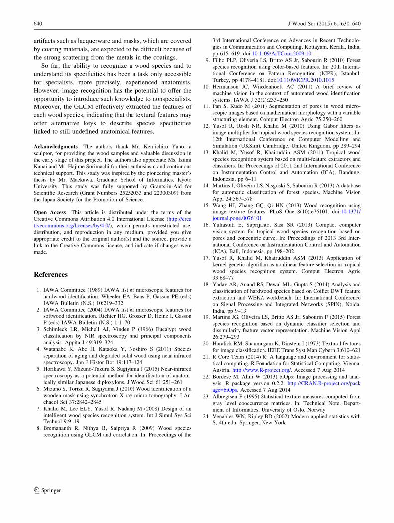
The predicted accuracies obtained using the parameters
‘‘average ? range’’ and ‘‘0�’’ are shown in Figs. 7 and 8,
respectively. In either case, the predicted accuracy was
greater than 0.99 for the initial dataset with the best quality,
indicating almost all images were classified into their true
classes. With a reduction in the resolution, the number of
gray levels, or the image size, the predicted accuracy
basically decreased. However, the number of gray levels
had a lower effect on the accuracy, except for eight gray
levels. The number of gray levels could be reduced to 16 or
32, which will be a great advantage to the system for
significant reductions in the calculation time and database
capacity. The resolution of 0.1 mm resulted in a high
predicted accuracy as did 0.05 mm, but the accuracy
Table 1 Optimum parameters for each condition
Image size
(cm2)
1.5 9 1.5 1 9 1 0.5 9 0.5
Resolution
(mm/pixel)
0.05 0.1 0.15 0.2 0.25 0.05 0.1 0.15 0.2 0.25 0.05 0.1 0.15 0.2 0.25
Gray level
8 a ? r 0� a ? r 0� 0� a ? r 0� a ? r 0� 0� a ? r a ? r a ? r a ? r 0�16 a ? r ave a ? r 0� 0� a ? r 0� a ? r 0� ave a ? r 0� a ? r 0� 0�32 a ? r ave a ? r 0� 0� a ? r 0� 0� 0� 0� a ? r 0� a ? r 0� 0�64 0�, 90�,
a ? r
90� a ? r a ? r ave 90� a ? r a ? r 0� 0� a ? r 0� a ? r 0� 0�
128 90� 90� a ? r 0� ave 90� a ? r a ? r 0� 0� ave 0� a ? r 0� ave
256 0�, 90�, ave 90�, ave a ? r 0� ave a ? r a ? r a ? r 0� 0� ave a ? r 0� 0� 0�, ave, a ? r
ave ‘‘average’’, a ? r ‘‘average ? range’’
J Wood Sci (2015) 61:630–640 637
123
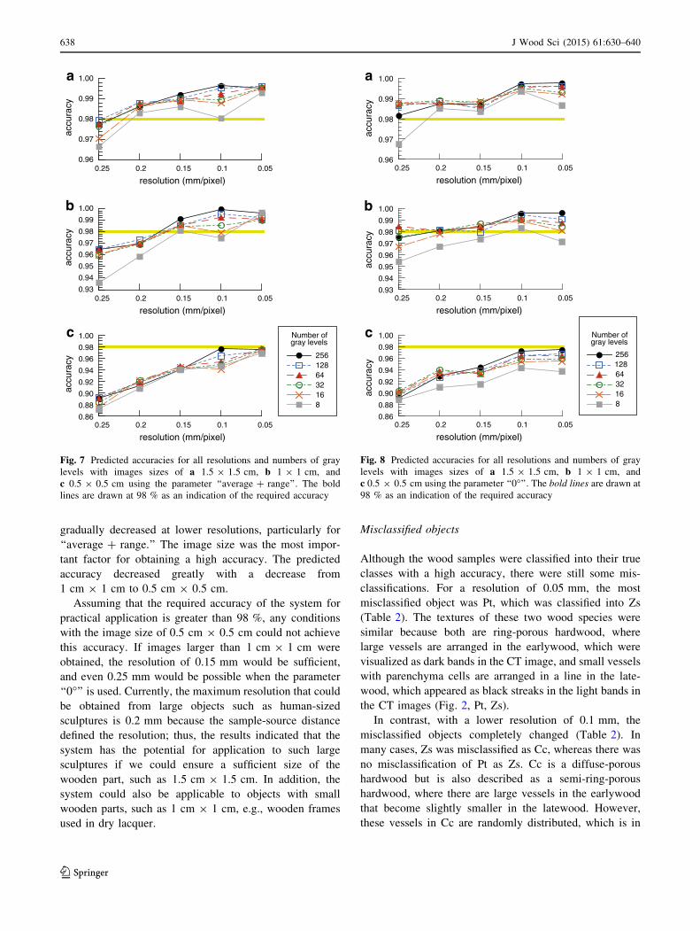
gradually decreased at lower resolutions, particularly for
‘‘average ? range.’’ The image size was the most impor-
tant factor for obtaining a high accuracy. The predicted
accuracy decreased greatly with a decrease from
1 cm 9 1 cm to 0.5 cm 9 0.5 cm.
Assuming that the required accuracy of the system for
practical application is greater than 98 %, any conditions
with the image size of 0.5 cm 9 0.5 cm could not achieve
this accuracy. If images larger than 1 cm 9 1 cm were
obtained, the resolution of 0.15 mm would be sufficient,
and even 0.25 mm would be possible when the parameter
‘‘0�’’ is used. Currently, the maximum resolution that could
be obtained from large objects such as human-sized
sculptures is 0.2 mm because the sample-source distance
defined the resolution; thus, the results indicated that the
system has the potential for application to such large
sculptures if we could ensure a sufficient size of the
wooden part, such as 1.5 cm 9 1.5 cm. In addition, the
system could also be applicable to objects with small
wooden parts, such as 1 cm 9 1 cm, e.g., wooden frames
used in dry lacquer.
Misclassified objects
Although the wood samples were classified into their true
classes with a high accuracy, there were still some mis-
classifications. For a resolution of 0.05 mm, the most
misclassified object was Pt, which was classified into Zs
(Table 2). The textures of these two wood species were
similar because both are ring-porous hardwood, where
large vessels are arranged in the earlywood, which were
visualized as dark bands in the CT image, and small vessels
with parenchyma cells are arranged in a line in the late-
wood, which appeared as black streaks in the light bands in
the CT images (Fig. 2, Pt, Zs).
In contrast, with a lower resolution of 0.1 mm, the
misclassified objects completely changed (Table 2). In
many cases, Zs was misclassified as Cc, whereas there was
no misclassification of Pt as Zs. Cc is a diffuse-porous
hardwood but is also described as a semi-ring-porous
hardwood, where there are large vessels in the earlywood
that become slightly smaller in the latewood. However,
these vessels in Cc are randomly distributed, which is in
0.99
1.00
0.050.10.150.20.250.96
0.97
0.98
0.20.250.93
0.94
0.95
0.96
0.97
0.98
0.99
1.00
0.050.10.15
resolution (mm/pixel)
accu
racy
resolution (mm/pixel)
resolution (mm/pixel)
2561286432168
Number ofgray levels
accu
racy
accu
racy
a
b
c
0.20.250.86
0.88
0.90
0.92
0.94
0.96
0.98
1.00
0.050.10.15
Fig. 7 Predicted accuracies for all resolutions and numbers of gray
levels with images sizes of a 1.5 9 1.5 cm, b 1 9 1 cm, and
c 0.5 9 0.5 cm using the parameter ‘‘average ? range’’. The bold
lines are drawn at 98 % as an indication of the required accuracy
resolution (mm/pixel)
resolution (mm/pixel)
resolution (mm/pixel)
a
b
c
0.96
0.97
0.98
0.99
1.00
0.050.10.150.20.25
0.86
0.88
0.90
0.92
0.94
0.96
0.98
1.00
0.050.10.150.20.25
0.93
0.94
0.95
0.96
0.97
0.98
0.99
1.00
0.050.10.150.20.25
2561286432168
Number ofgray levels
accu
racy
accu
racy
accu
racy
Fig. 8 Predicted accuracies for all resolutions and numbers of gray
levels with images sizes of a 1.5 9 1.5 cm, b 1 9 1 cm, and
c 0.5 9 0.5 cm using the parameter ‘‘0�’’. The bold lines are drawn at
98 % as an indication of the required accuracy
638 J Wood Sci (2015) 61:630–640
123

contrast to Zs, a representative ring-porous hardwood with
a single row of large vessels in the pore zone and a tan-
gential arrangement of latewood vessels. This difference in
the distribution of the vessels enabled clear discrimination
with a resolution of 0.05 mm. In fact, the CT images of Cc
with a resolution of 0.05 mm exhibited local gray-level
variations corresponding to the vessels, whereas those of
Zs exhibited little variation in the earlywood because of the
densely arranged vessels in the pore zone (Fig. 2, Cc, Zs).
With a reduction in the resolution to 0.1 mm; however,
such a difference was hardly detected, and the regions of
earlywood in Cc also exhibited dark colors with little
variation, which made it similar to Zs.
To eliminate these errors, we have to revise each step in
the system. In terms of the image dataset or the pretreat-
ment of images, calibration of the gray levels to the actual
density of wood seems to be a quite efficient and reliable
approach because the specific gravities of the wood sam-
ples are actually quite different; in particular, Pt is known
as a significantly light wood. Regarding feature extraction,
the use of a multifeature extractor by combining the GLCM
analysis with other filtering and transforms seems
promising to improve the recognition accuracy. For
example, feature extraction methods that focused on the
periodicity of the images, such as the FFT and Gabor filter,
would be effective for recognizing the differences between
Cc and Zs because Zs has a clear periodicity in the radial
direction derived from the tangential arrangement of the
latewood vessels compared to Cc. The periodicity in the
radial direction derived from the ray may also be possibly
detected and contribute to the improvement in the system.
Conclusion
We constructed a novel system for wood identification
from low-resolution CT data using the GLCM and k-NN
algorithm as a feature extractor and classifier, respectively.
The system recognized 10 wood samples almost perfectly,
although it is necessary to continue improvement. The
current system is still at the level of individual recognition
because the data were obtained from one wood block for
each species; thus, data from multiple individuals should be
added to the database to advance to the level of species
recognition. In addition, the applicability of the system to
various practical situations should be tested further;
Table 2 Classification table for
five different numbers of gray
levels (16, 32, 64, 128, and
256), five k values (1, 3, 5, 7,
and 9), and two parameters
(‘‘0�’’ and ‘‘average ? range’’)
for an image size of 3 9 3 cm
True class
Cc Ce Cj1 Cj2 Co1 Co2 Mo Pt Tn Zs
Resolution of 0.05 mm
Classified class (%)
Cc 100 0 0 0 0 0.10 0 0 0 0.50
Ce 0 100 0 0 0 0 0 0 0 0
Cj1 0 0 99.35 0 0 0 0 0 0 0
Cj2 0 0 0 100 0 0.50 0 0 0 0
Co1 0 0 0.65 0 100 0 0 0 0 0
Co2 0 0 0 0 0 99.30 0 0 0 0
Mo 0 0 0 0 0 0 100 0 0 0
Pt 0 0 0 0 0 0 0 97.50 0 0.30
Tn 0 0 0 0 0 0 0 0 100 0
Zs 0 0 0 0 0 0.10 0 2.50 0 99.20
Resolution of 0.1 mm
Classified class (%)
Cc 99.40 0 0 0 0 0.90 0 0.10 0 4.30
Ce 0 100 0 0 0 0 0 0 0 0
Cj1 0 0 100 0 0 0 0 0 0 0
Cj2 0 0 0 100 0 0.25 0 0 0 0
Co1 0 0 0 0 100 0 0 0 0 0
Co2 0 0 0 0 0 98.85 0 0 0 0
Mo 0 0 0 0 0 0 100 0 0 0
Pt 0 0 0 0 0 0 0 99.90 0 0
Tn 0 0 0 0 0 0 0 0 100 0
Zs 0.60 0 0 0 0 0 0 0 0 95.70
J Wood Sci (2015) 61:630–640 639
123
artifacts such as lacquerware and masks, which are covered
by coating materials, are expected to be difficult because of
the strong scattering from the metals in the coatings.
So far, the ability to recognize a wood species and to
understand its specificities has been a task only accessible
for specialists, more precisely, experienced anatomists.
However, image recognition has the potential to offer the
opportunity to introduce such knowledge to nonspecialists.
Moreover, the GLCM effectively extracted the features of
each wood species, indicating that the textural features may
offer alternative keys to describe species specificities
linked to still undefined anatomical features.
Acknowledgments The authors thank Mr. Ken’ichiro Yano, a
sculptor, for providing the wood samples and valuable discussion in
the early stage of this project. The authors also appreciate Ms. Izumi
Kanai and Mr. Hajime Sorimachi for their enthusiasm and continuous
technical support. This study was inspired by the pioneering master’s
thesis by Mr. Maekawa, Graduate School of Informatics, Kyoto
University. This study was fully supported by Grants-in-Aid for
Scientific Research (Grant Numbers 25252033 and 22300309) from
the Japan Society for the Promotion of Science.
Open Access This article is distributed under the terms of the
Creative Commons Attribution 4.0 International License (http://crea
tivecommons.org/licenses/by/4.0/), which permits unrestricted use,
distribution, and reproduction in any medium, provided you give
appropriate credit to the original author(s) and the source, provide a
link to the Creative Commons license, and indicate if changes were
made.
References
1. IAWA Committee (1989) IAWA list of microscopic features for
hardwood identification. Wheeler EA, Baas P, Gasson PE (eds)
IAWA Bulletin (N.S.) 10:219–332
2. IAWA Committee (2004) IAWA list of microscopic features for
softwood identification. Richter HG, Grosser D, Heinz I, Gasson
P (eds) IAWA Bulletin (N.S.) 1:1–70
3. Schimleck LR, Michell AJ, Vinden P (1966) Eucalypt wood
classification by NIR spectroscopy and principal components
analysis. Appita J 49:319–324
4. Watanabe K, Abe H, Kataoka Y, Noshiro S (2011) Species
separation of aging and degraded solid wood using near infrared
spectroscopy. Jpn J Histor Bot 19:117–124
5. Horikawa Y, Mizuno-Tazuru S, Sugiyama J (2015) Near-infrared
spectroscopy as a potential method for identification of anatom-
ically similar Japanese diploxylons. J Wood Sci 61:251–261
6. Mizuno S, Torizu R, Sugiyama J (2010) Wood identification of a
wooden mask using synchrotron X-ray micro-tomography. J Ar-
chaeol Sci 37:2842–2845
7. Khalid M, Lee ELY, Yusof R, Nadaraj M (2008) Design of an
intelligent wood species recognition system. Int J Simul Sys Sci
Technol 9:9–19
8. Bremananth R, Nithya B, Saipriya R (2009) Wood species
recognition using GLCM and correlation. In: Proceedings of the
3rd International Conference on Advances in Recent Technolo-
gies in Communication and Computing, Kottayam, Kerala, India,
pp 615–619. doi:10.1109/ArTCom.2009.10
9. Filho PLP, Oliveria LS, Britto AS Jr, Sabourin R (2010) Forest
species recognition using color-based features. In: 20th Interna-
tional Conference on Pattern Recognition (ICPR), Istanbul,
Turkey, pp 4178–4181. doi:10.1109/ICPR.2010.1015
10. Hermanson JC, Wiiedenhoeft AC (2011) A brief review of
machine vision in the context of automated wood identification
systems. IAWA J 32(2):233–250
11. Pan S, Kudo M (2011) Segmentation of pores in wood micro-
scopic images based on mathematical morphology with a variable
structuring element. Comput Electron Agric 75:250–260
12. Yusof R, Rosli NR, Khalid M (2010) Using Gabor filters as
image multiplier for tropical wood species recognition system. In:
12th International Conference on Computer Modelling and
Simulation (UKSim), Cambridge, United Kingdom, pp 289–294
13. Khalid M, Yusof R, Khairuddin ASM (2011) Tropical wood
species recognition system based on multi-feature extractors and
classifiers. In: Proceedings of 2011 2nd International Conference
on Instrumentation Control and Automation (ICA), Bandung,
Indonesia, pp 6–11
14. Martins J, Oliveira LS, Nisgoski S, Sabourin R (2013) A database
for automatic classification of forest species. Machine Vision
Appl 24:567–578
15. Wang HJ, Zhang GQ, Qi HN (2013) Wood recognition using
image texture features. PLoS One 8(10):e76101. doi:10.1371/
journal.pone.0076101
16. Yuliastuti E, Suprijanto, Sasi SR (2013) Compact computer
vision system for tropical wood species recognition based on
pores and concentric curve. In: Proceedings of 2013 3rd Inter-
national Conference on Instrumentation Control and Automation
(ICA), Bali, Indonesia, pp 198–202
17. Yusof R, Khalid M, Khairuddin ASM (2013) Application of
kernel-genetic algorithm as nonlinear feature selection in tropical
wood species recognition system. Comput Electron Agric
93:68–77
18. Yadav AR, Anand RS, Dewal ML, Gupta S (2014) Analysis and
classification of hardwood species based on Coiflet DWT feature
extraction and WEKA workbench. In: International Conference
on Signal Processing and Integrated Networks (SPIN), Noida,
India, pp 9–13
19. Martins JG, Oliveira LS, Britto AS Jr, Sabourin F (2015) Forest
species recognition based on dynamic classifier selection and
dissimilarity feature vector representation. Machine Vision Appl
26:279–293
20. Haralick RM, Shanmugam K, Dinstein I (1973) Textural features
for image classification. IEEE Trans Syst Man Cybern 3:610–621
21. R Core Team (2014) R: A language and environment for statis-
tical computing. R Foundation for Statistical Computing, Vienna,
Austria. http://www.R-project.org/. Accessed 7 Aug 2014
22. Bordese M, Alini W (2013) biOps: Image processing and anal-
ysis. R package version 0.2.2. http://CRAN.R-project.org/pack
age=biOps. Accessed 7 Aug 2014
23. Albregtsen F (1995) Statistical texture measures computed from
gray level cooccurrence matrices. In: Technical Note, Depart-
ment of Informatics, University of Oslo, Norway
24. Venables WN, Ripley BD (2002) Modern applied statistics with
S, 4th edn. Springer, New York
640 J Wood Sci (2015) 61:630–640
123