automated knowledge based filter synthesis using
TRANSCRIPT
ELEKTRONIKA IR ELEKTROTECHNIKA, ISSN 1392-1215, VOL. 19, NO. 9, 2013
Abstract—This work gives an original algorithm that
combines design and synthesis step with the optimization for
targeted implementation technology. The approximation step is
based on Gegenbauer polynomial and the corresponding cost
function. The proposed methodology is an example of usage of
computer algebra system as an alternative to classic numeric
computing.
Index Terms—Analog integrated circuits, circuit analysis
computing, design for manufacture, elliptic design.
I. INTRODUCTION
Analog filters are frequency-selective electrical circuits
that are used to amplify or attenuate the band-limited signal
frequency spectrum [1]. Many different physical components
can be used for implementation. In practice, the values of
filter components diverge from the ideal and the results of
filtering may be different from the expected frequency
response. The different technologies are impaired with
different types of errors in the components. An exhaustive
research on active components is presented in [2]. It is
important to choose a filter structure with a low sensitivity to
the expected dominant errors in the intended implementation
technology. For example, the elliptic digital filter is the most
efficient filter because there is no other filter of the lower
order that can fulfill the same filter specification [1]. The
EMQF (Elliptic Minimum Q Factor) filters are the most
efficient filters of the elliptic filters [3]. The design
procedure of the EMQF digital filters is presented in [4].
The similar design strategy was implemented for analog
filters implemented in SC (Switched Capacitor) technology
[5].
The design of high performance digital signal processing
circuits can be very efficient using digital programmable
circuits as it is shown in [4], [6], and [7]. Quite different
design procedure should be followed when analog
programmable circuits are used with on-chip tuning [8]. The
most important strategy is the optimization of the second
Manuscript received September 26, 2012; accepted August 26, 2013.
This work was partially supported by the Ministry of Education,
Science and Technological Development of Serbia under Grant TR-32023.
order sections [9].
In this paper, a new synthesis strategy is presented based
on knowledge inputted into CAS (Computer Algebra
System) [10]. The method is based on all-pole
approximation technique and formulation of the cost
function that minimizes the difference of the maximal pole-
Q factor of the transfer function from the set of preferred Q
factors available in programmable analog circuits.
II. APPROXIMATION
The even-order low-pass prototype all-pole filter transfer
function can be represented using the pole frequencies, ,p k
(or the corner frequency, , / 2ck p kf ), the pole Q-
factors, ,p kQ , and the filter order n
/22
,1
/2,2 2
,,1
( ) .
( )
n
p kk
n np k
p kp kk
H s
s sQ
(1)
The squared magnitude response can be expressed using
the even-order polynomial approximation, 2 ( )nA , and the
ripple factor,
222
1( ) ( ) , ( ) 1, 1.
1 ( )n n n
n
H j H j AA
(2)
The synthesis means to find the procedure for computing
the squared pole frequencies, ,p k , and the pole Q-factors,
,p kQ , for 1, 2, 3,..., / 2)k n , starting from (2) and to
achieve parameters of the programmable integrated circuits
with the minimal error of the designed transfer function for
the specified filter specification. We choose all-pole transfer
function in order to avoid an additional element for
implementing zeros of the transfer function. Actually, we
will try to optimize the maximal Q factor because it is the
most critical element, and at the same time to fulfill filter
specification and the implementation requirements of the
Automated Knowledge Based Filter Synthesis
Using Gegenbauer Approximation and
Optimization of Pole-Q Factors
M. Lutovac1, V. Pavlovic2, M. Lutovac3 1Lola Institute, Kneza Viseslava 70a, 11000 Belgrade, Serbia,
2Faculty of Electronic Engineering Niš. Aleksandra Medvedeva 14, 18000 Niš, Serbia 3Singidunum University Belgrade, Danijelova 32, 11000 Belgrade, Serbia,
http://dx.doi.org/10.5755/j01.eee.19.9.2516
97
ELEKTRONIKA IR ELEKTROTECHNIKA, ISSN 1392-1215, VOL. 19, NO. 9, 2013
targeted technology.
The squared magnitude response of the proposed filter
class is based on the even-order Gegenbauer orthogonal
polynomials, 2 ( )rG [11], and it is normalized to the unity
value at the pass-band edge frequency, 2 (1) 1nA
2
2 20
2 2
2 20
( )
( )
(1)
n
r rr
n n
r rr
b G
A
b G
. (3)
The cost function can be represented using the weight
function 2 1/2( ) (1 )p , the design parameters (the
filter coefficients 0b , 2b , 4b , 6, 2..., nb b , and the two free
normalizing parameters, 1 and 2 ), and the even-order
Gegenbauer orthogonal polynomials
40 2 6 2 0 1
12 1/2 2
2 200
0 2 2 1 2 20 0
( , , , , . . . , , )
(1 ) [ ( ) ] ( )
[ (0) ] [ (1) 1].
n
r n
r rr
r n r n
r r r rr r
b b b b b
b G d
b G b G
(4)
The optimal values are computed by solving the system of
equations in which the first partial derivatives of the cost
function with respect to the design parameters are equal to 0,
that is 2d / d 0ib , and d / d 0i .
The closed-form solution is rather complicated even for
experienced users, and the whole procedure is implemented
using computer algebra system [10].
The squared norm, rh , of the orthogonal Gegenbauer
polynomial 2 ( ), 0, 1, 2, 3,...rG r is defined
1
2 20
( ) ( ) ( ) ( ), 0, 1, ...r r rh p G G d r (5)
The integration gives the values of rh in terms of r, the
weighting parameter and the Pochamer symbol 2(2 ) r
2
1 1(2 ) ( ) ( )
2 2( ) , 0, 1, 2,3,...(2 )!( 2 ) ( )
r
rh rr r
(6)
The design procedure is explained by the example in the
next section. Notice that filter specification can be given
using the reflection factor
2
2
2.
1
(7)
The design algorithm is implemented in software
Mathematica [10].
III. BUILDING KNOWLEDGE FOR SYNTHESIS
Some software tools already have special functions that
are required for the filter design. Since we are going to
prepare template notebook, we present the code in
Mathematica [10] software as one of the best CAS software.
Firstly, the formulas are inputted into CAS software.
The first cells contain the minimal number of parameters
such as the number of biquads (nBiquads=5) and auxiliary
weighting factor (v0=1/2) for computing all other values:
nBiquads = 5;
n = 2 nBiquads;
b = Table[ToExpression[StringJoin["b",
ToString[r]]], {r, 0, 2 n, 2}]
v0 = 1/2
The list of coefficients b is automatically generated:
{b0,b2,b4,b6,b8,b10,b12,b14,b16,b18,b20}
The code of the squared magnitude response is similar to
(3):
The code for the cost function is also very similar to the
definition (4), except that the name of the special function is
not the Gegenbauer polynomial but unknown function pP:
After defining the cost function in CAS, the next step
is to find the first partial derivatives of the cost function with
respect to the design parameters. The Gegenbauer
polynomials can be treated as constants and the integration
can be performed after derivation. One of the key features of
CAS is that it is not necessary to specify exact values of
variables on the right side of an equation, but the symbolic
name can be used instead. Since we have three different
expressions of the Gegenbauer polynomials, the same
number of substitution rules is specified:
sub0= pP[x_,v_,0] → GegenbauerC[x, v, 0];
sub1= pP[x_,v_,1] → GegenbauerC[x, v, 1];
subw= pP[x_,v_,w_] → GegenbauerC[x, v, w];
Now, we can create a set of equations that are generated
using partial derivatives (actually only left side of
equations):
eqB=Table[D[ , b[[r+1]]],{r,0,n}]/. sub0 /. sub1
/. subw /. v → v0;
eqL = {D[ ,L0]/. sub0/. sub1/. subw/. v→v0,
D[ ,L1]/. sub0/. sub1/. subw/. v→v0};
The whole processing time is much larger when the
98
ELEKTRONIKA IR ELEKTROTECHNIKA, ISSN 1392-1215, VOL. 19, NO. 9, 2013
substitution of the Gegenbauer polynomials is performed
before derivation. The two matrices are joined in one and
symbolic description for equating to 0 is added to the each
row:
eqLeft = Join[eqB, eqL];
eqs=Thread[eqLeft==0];
parameters=Join[b,{L0,L1}]
After forming the system of equations eqs and the list of
all parameters parameters, the solutions are computed
using built-in command Solve. The solutions are in the
form of replacement rules sol1, which can be used in earlier
defined squared magnitude function aw:
sol1 = Solve[eqs, parameters]
aw = a2/.sol1;
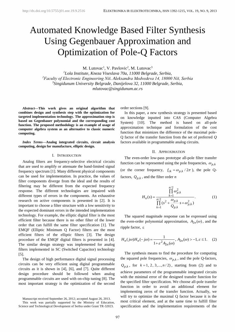
Fig. 1. Polynomial approximation for 10n , 0.5 , 2 ( ) -2.47nA
2 4 6 20 111 1712.6 22318 .
Figure 1 illustrates the computed squared magnitude
function. It is important to notice that only the number of
biquads is defined and the value of weighting factor. For any
other number of biquads or another value of weighting
factor, the same notebook can be evaluate after changing the
two numeric values in the first input cell.
The rest of the notebook can be prepared in a similar way.
The denominator of (2) is defined for the specified ripple
factor or the preferred reflection factor, say =1/10. The
roots are in quadruplet and only the left half plane roots are
selected to form the poles of the transfer function.
Multiplying the two consecutive complex-conjugate roots
the squared pole magnitude is computed, and using the
definition of the pole Q factor [1] the Q factors of each
biquad can be computed.
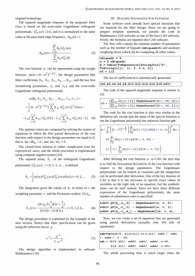
Fig. 2. Attenuation of the filter 2
1010log ( )nA H j in dB for
10n , 0.5 , =0.1.
Finally, a list of the biquad transfer functions is carried
out:
The attenuation is computed and shown in Fig. 2 and
Fig. 3.
Fig. 3. Attenuation of the filter in the pass-band for 10n , 0.5 ,
=0.1.
IV. POLE Q-FACTOR OPTIMIZATION
Commonly, the filter design generates transfer function
from the filter specification and at least one of the
parameters is better than required [1]. We can use that
parameter for the optimization and to improve some
characteristics. For example, the stop-band attenuation can
be higher than specified. Instead of redesigning the filter,
that can be time consuming, we can optimize one of the
design parameters. In this paper, we are changing the
weighting factor until we have the exact value of the critical
Q factor from the set of available values.
The optimization procedure is as follows: firstly, we
determine the range of the weighting factors for that the
pass-band and stop-band attenuations fulfill filter
specification. Next, we determine the pole-Q-factor as a
function of the weighting factor. Finally, by equating the
function with one or more values from the available values
specified by manufacturer, we find values of the weighting
factor.
For example, suppose that the filter specifications are
fulfilled for the weighting factor from the range of values
{0.1. 0.2}. Since the filter design knowledge already exists
in computer algebra system, the redesign process can be
simplified. The basic idea is not to find a minimal value of
the pole-Q-factor, but to design a filter that has an exact
predefined value of the maximal pole-Q-factor, for example
a value from the set of possible values available from
programmable analog integrated circuits [7]. Using fitting
function, we can derive a closed form approximation of the
critical Q-factor (the largest Q-factor) in terms of the
parameter . The closed form approximation can be
presented in a polynomial form. Solving the equation
setQ Q we can derive the parameter in terms of the
specified Q-factor. In this case, for the preferred value of the
critical Q-factor 9setQ , the value of the weighting factor
is 0.125198. The next step is to find the optimal sequence of
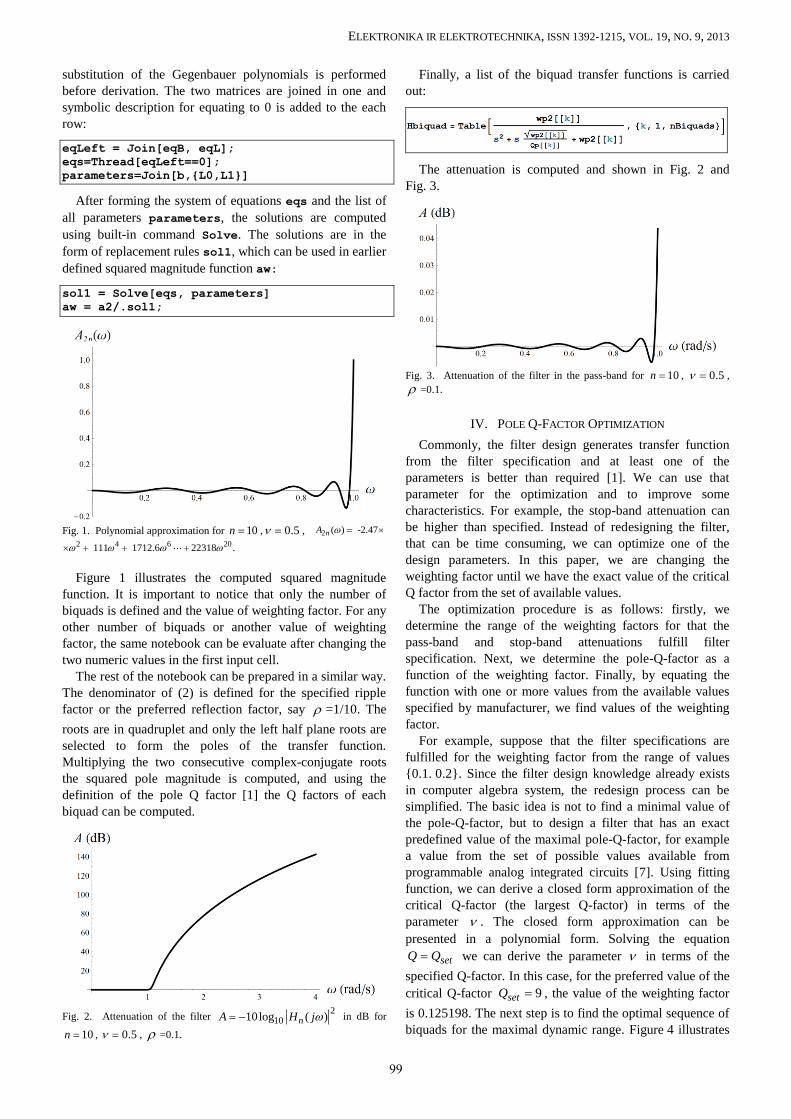
biquads for the maximal dynamic range. Figure 4 illustrates
99
ELEKTRONIKA IR ELEKTROTECHNIKA, ISSN 1392-1215, VOL. 19, NO. 9, 2013
an example of the implementation using programmable chip
(AN221E04 device) that is designed using
AnadigmDesigner software. Four biquads are placed in a
chip, while the fifth one is in another chip. The implemented
corner frequencies and the corresponding Q factors are
shown with each biquad.
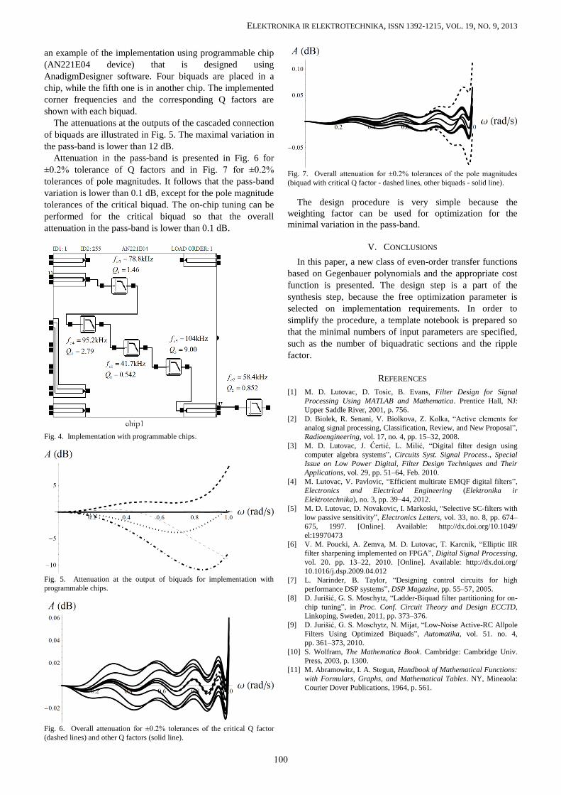
The attenuations at the outputs of the cascaded connection
of biquads are illustrated in Fig. 5. The maximal variation in
the pass-band is lower than 12 dB.
Attenuation in the pass-band is presented in Fig. 6 for
±0.2% tolerance of Q factors and in Fig. 7 for ±0.2%
tolerances of pole magnitudes. It follows that the pass-band
variation is lower than 0.1 dB, except for the pole magnitude
tolerances of the critical biquad. The on-chip tuning can be
performed for the critical biquad so that the overall
attenuation in the pass-band is lower than 0.1 dB.
Fig. 4. Implementation with programmable chips.
Fig. 5. Attenuation at the output of biquads for implementation with
programmable chips.
Fig. 6. Overall attenuation for ±0.2% tolerances of the critical Q factor
(dashed lines) and other Q factors (solid line).
Fig. 7. Overall attenuation for ±0.2% tolerances of the pole magnitudes
(biquad with critical Q factor - dashed lines, other biquads - solid line).
The design procedure is very simple because the
weighting factor can be used for optimization for the
minimal variation in the pass-band.
V. CONCLUSIONS
In this paper, a new class of even-order transfer functions
based on Gegenbauer polynomials and the appropriate cost
function is presented. The design step is a part of the
synthesis step, because the free optimization parameter is
selected on implementation requirements. In order to
simplify the procedure, a template notebook is prepared so
that the minimal numbers of input parameters are specified,
such as the number of biquadratic sections and the ripple
factor.
REFERENCES
[1] M. D. Lutovac, D. Tosic, B. Evans, Filter Design for Signal
Processing Using MATLAB and Mathematica. Prentice Hall, NJ:
Upper Saddle River, 2001, p. 756.
[2] D. Biolek, R. Senani, V. Biolkova, Z. Kolka, “Active elements for
analog signal processing, Classification, Review, and New Proposal”,
Radioengineering, vol. 17, no. 4, pp. 15–32, 2008.
[3] M. D. Lutovac, J. Ćertić, L. Milić, “Digital filter design using
computer algebra systems”, Circuits Syst. Signal Process., Special
Issue on Low Power Digital, Filter Design Techniques and Their
Applications, vol. 29, pp. 51–64, Feb. 2010.
[4] M. Lutovac, V. Pavlovic, “Efficient multirate EMQF digital filters”,
Electronics and Electrical Engineering (Elektronika ir
Elektrotechnika), no. 3, pp. 39–44, 2012.
[5] M. D. Lutovac, D. Novakovic, I. Markoski, “Selective SC-filters with
low passive sensitivity”, Electronics Letters, vol. 33, no. 8, pp. 674–
675, 1997. [Online]. Available: http://dx.doi.org/10.1049/
el:19970473
[6] V. M. Poucki, A. Zemva, M. D. Lutovac, T. Karcnik, “Elliptic IIR
filter sharpening implemented on FPGA”, Digital Signal Processing,
vol. 20. pp. 13–22, 2010. [Online]. Available: http://dx.doi.org/
10.1016/j.dsp.2009.04.012
[7] L. Narinder, B. Taylor, “Designing control circuits for high
performance DSP systems”, DSP Magazine, pp. 55–57, 2005.
[8] D. Jurišić, G. S. Moschytz, “Ladder-Biquad filter partitioning for on-
chip tuning”, in Proc. Conf. Circuit Theory and Design ECCTD,
Linkoping, Sweden, 2011, pp. 373–376.
[9] D. Jurišić, G. S. Moschytz, N. Mijat, “Low-Noise Active-RC Allpole
Filters Using Optimized Biquads”, Automatika, vol. 51. no. 4,
pp. 361–373, 2010.
[10] S. Wolfram, The Mathematica Book. Cambridge: Cambridge Univ.
Press, 2003, p. 1300.
[11] M. Abramowitz, I. A. Stegun, Handbook of Mathematical Functions:
with Formulars, Graphs, and Mathematical Tables. NY, Mineaola:
Courier Dover Publications, 1964, p. 561.
100