T E C H N I C A L

R E P O R T

11002

Ideal denoising within a family of tree-structured

wavelet estimators

AUTIN, F., FREYERMUTH, J.-M. and R. von SACHS

*

I A P S T A T I S T I C S

N E T W O R K

INTERUNIVERSITY ATTRACTION POLE

http://www.stat.ucl.ac.be/IAP

Ideal Denoising within a Family of Tree-Structured

Wavelet Estimators

Florent Autin ∗ Jean-Marc Freyermuth † Rainer von Sachs ‡

January 7, 2011

Abstract

We focus on the performances of tree-structured wavelet estimators belonging to a largefamily of keep-or-kill rules, namely the Vertical Block Thresholding family. For each estima-tor, we provide the maximal functional space (maxiset) for which the quadratic risk reachesa given rate of convergence. Following a discussion on the maxiset embeddings, we identifythe ideal estimator of this family, that is the one associated with the largest maxiset. Weemphasize the importance of such a result since the ideal estimator is different from theusual (plug-in) estimator used to mimic the performances of the Oracle. Finally, we confirmour theoretical results through extensive numerical experiments.

Keywords : Besov spaces, wavelet-based estimation, CART, maxiset and oracle approaches, rateof convergence, thresholding methods, tree structure

∗Université d’Aix-Marseille 1, CNRS UMR 6632,C.M.I., 39 rue F. Joliot Curie, 13453 Marseille Cedex 13.Email: autin@cmi.univ-mrs.fr. Research partly supported by A.N.R. project Oracle.

†Université catholique de Louvain, Institut de statistique, Voie du Roman Pays, 20, B-1348 Louvain-la-Neuve,Belgium. Email: Jean-Marc.Freyermuth@uclouvain.be. Financial support from the contract "Projet d’Actionsde Recherche Concertées" nr. 07/12/002 of the "Communauté française de Belgique", granted by the "Académieuniversitaire Louvain", is gratefully acknowledged.

‡Université catholique de Louvain, Institut de statistique, Voie du Roman Pays, 20, B-1348 Louvain-la-Neuve,Belgium. Email: rvs@uclouvain.be. Financial support from the contract "Projet d’Actions de Recherche Con-certées" nr. 07/12/002 of the "Communauté française de Belgique", granted by the "Académie universitaireLouvain", is gratefully acknowledged.

1

1 Introduction

Wavelet methods are known to be powerful in nonparametric estimation of functions. Indeed,the information of a function is localized in a few large wavelet coefficients for a wide range offunction classes. This is the key-point to understand why hard and soft thresholding methodsperform well. These methods introduced by Donoho and Johnstone (12) consist in estimatingthe function by using the empirical wavelet coefficients which are larger than a chosen thresholdvalue. In particular, these estimators were shown to be near optimal over Besov spaces while theyare adaptive for the regularity parameter (see Donoho and Johnstone (12; 13)). As mentioned byAutin (3) such thresholding rules are elitist in the sense that small empirical wavelet coefficientsare not used in the reconstruction of the function.

Recent developments in wavelet thresholding have shown that elitist procedures can be outper-formed in both theoretical and practical way by methods which refine the choice of the waveletcoefficients to be used in the reconstruction. This refined choice makes use of information fromneighbored coefficients, e.g., block thresholding methods (see among others Cai (8), Autin (3; 5))or impose that the empirical coefficients used for the reconstruction of the signal are arrangedover a rooted connected tree (see Baraniuk (7), Cohen et al. (9), Autin (4)). We denote thelatter as Tree Structured Wavelets (TSW) estimators. Interest in TSW already appeared in theworks of Donoho (13) and Engel (14), (15). In particular they pointed out the connection be-tween TSW and CART. Actually, TSW benefit from interest in various literature ranging fromdata compression to image processing and statistics where, in the context of curve denoising,they have already shown their potential compared to fully nonlinear methods (see among othersJansen (18), Lee (19), Autin (4), Freyermuth et al. (16)). However, this paper is not in the lineto compare TSW to other well established methods. Its aim is rather to emphasize an importantaspect about the selection of the ideal procedure among a ’natural’ family of TSW estimators.The family of estimators that we will consider includes as special cases two popular TSW esti-mators, the CART-like estimator obtained by model selection (see Donoho (13) and Engel(14)) and the Hard Tree estimator (see Autin(4))).

The Figures 1-4 show an example of a reconstruction of the Blip function using these methods(defined in Section 3) and the associated wavelet coefficient magnitudes (the darker the largerthe coefficient magnitude).

2

Figure 1: True function. Figure 2: Noisy data.

Figure 3: CART-like estimator. Figure 4: Hard Tree estimator.

Looking at the positions of the large wavelet coefficients in the Figure 1, we notice a hierarchi-cal structure between them. In particular, there are large wavelet coefficients that persist acrossscales at the location of the singularity. The two methods of reconstruction give estimators in theFigures 3 and 4 which appear to be close to the target function. Note that the sets of empiricalwavelet coefficients used by the two methods are embedded (see Proposition 3.1). In particular,the cardinality of the set of empirical coefficients used in the reconstruction of the CART-likeestimator (Figure 3) is smaller than the one of the Hard Tree (Figure 4), quantitative resultsof section 6 support this remark. These facts will be discussed and interpreted throughout thepaper.

Donoho (13) proves that estimation under tree constraints can be solved by a CART-like al-gorithm. A Tree-Oracle estimator is obtained after a recursive-per-level method based on the

3

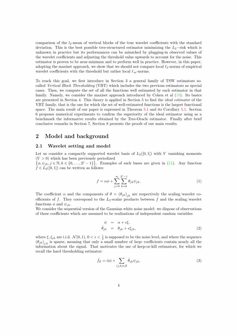
comparison of the l2-mean of vertical blocks of the true wavelet coefficients with the standarddeviation. This is the best possible tree-structured estimator minimizing the L2−risk which isunknown in practice but its performances can be mimicked by plugging-in observed values ofthe wavelet coefficients and adjusting the threshold value upwards to account for the noise. Thisestimator is proven to be near-minimax and to perform well in practice. However, in this paper,adopting the maxiset approach, we show that we should not compare local ℓ2-norms of empiricalwavelet coefficients with the threshold but rather local ℓ∞-norms.

To reach this goal, we first introduce in Section 3 a general family of TSW estimators so-called Vertical Block Thresholding (VBT) which includes the two previous estimators as specialcases. Then, we compute the set of all the functions well estimated by each estimator in thatfamily. Namely, we consider the maxiset approach introduced by Cohen et al (10). Its basicsare presented in Section 4. This theory is applied in Section 5 to find the ideal estimator of theVBT family, that is the one for which the set of well-estimated functions is the largest functionalspace. The main result of our paper is expressed in Theorem 5.1 and its Corollary 5.1. Section6 proposes numerical experiments to confirm the superiority of the ideal estimator using as abenchmark the informative results obtained by the Tree-Oracle estimator. Finally after briefconclusive remarks in Section 7, Section 8 presents the proofs of our main results.

2 Model and background

2.1 Wavelet setting and model

Let us consider a compactly supported wavelet basis of L2([0, 1]) with V vanishing moments(V > 0) which has been previously periodized{

φ, ψjk, j ∈ N, k ∈ {0, . . . , 2j − 1}}

. Examples of such bases are given in (11). Any functionf ∈ L2([0, 1]) can be written as follows:

f = αφ+

∞∑

j=0

2j−1∑

k=0

θjkψjk. (1)

The coefficient α and the components of θ = (θjk)jk are respectively the scaling/wavelet co-

efficients of f . They correspond to the L2-scalar products between f and the scaling/waveletfunctions φ and ψjk.We consider the sequential version of the Gaussian white noise model: we dispose of observationsof these coefficients which are assumed to be realizations of independent random variables:

α̂ = α+ ǫξ,

θ̂jk = θjk + ǫξjk, (2)

where ξ, ξjk are i.i.d. N (0, 1), 0 < ǫ < 12 is supposed to be the noise level, and where the sequence

(θjk)j,k is sparse, meaning that only a small number of large coefficients contain nearly all theinformation about the signal. That motivates the use of keep-or-kill estimators, for which werecall the hard thresholding estimator:

f̂S = α̂φ+∑

(j,k)∈Sθ̂jkψjk, (3)

4

where S ={

(j, k) ; 0 ≤ j < jλǫ; 0 ≤ k < 2j ;

∣

∣

∣θ̂jk

∣

∣

∣> λǫ

}

forms an unstructured set of indices of

’large’ wavelet coefficients (in the sequel, by ’large’ coefficients, we understand those which belongto S). Here,

• λǫ = m ǫ√

log(ǫ−1), m ∈ ( 0,∞ ],

• jλ is the integer such that 2−jλ ≤ λ2 < 21−jλ (0 < λ < 1). Here, jλǫis the finest level up

to which we consider the empirical wavelet coefficients to reconstruct the signal f .

This term by term thresholding does not take into account the information that give us theclusters of wavelet coefficients that we observed in the Figure 1. But this knowledge has thepractical application that, on the one hand, we would not use in the reconstruction a largeisolated wavelet coefficient because it is not likely to be part of the signal; on the other hand, asmall coefficient in the neighborhood of large coefficients would be kept. This motivates the useof refined thresholding methods such as the tree-structured wavelets (Autin (4) and Baraniuk(7)) which we describe in the next section.

2.2 Tree-structured wavelet estimators

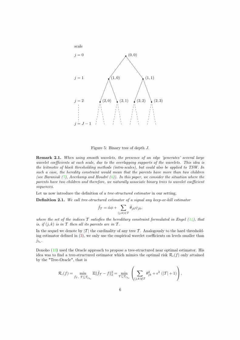
Tree-structured wavelet (TSW) estimators are based on the hierarchical interpretation of thewavelet expansion (1). The periodized wavelets {ψjk}jk are arranged over a nested multiscalestructure such that the support of each ψjk contains the supports of ψj+1,2k and ψj+1,2k+1. Thisinduces a hierarchy among the wavelet coefficients which can be represented over a binary treerooted in (0, 0) (see Figure 5). Hence, at the location of a singularity in the signal, we observethe persistence of large wavelet coefficients over all scales (see Figure 1).

Therefore, considering the wavelet coefficients as a multiresolution sequence provides additionalinformation which we aim to benefit from by imposing a tree/hereditary constraint. The hered-itary constraint requires that the set of non zero wavelet coefficients after thresholding forms aconnected rooted subtree. In other words, it cannot include an empirical wavelet coefficient unlessall its parents (defined in equation (4) below) are large.

We denote as TJ the binary tree of depth J for which the nodes are the couples of indices(

(j, k), 0 ≤ j < J, k ∈ {0, . . . , 2j − 1})

(see the Figure 5). For any couple of indices (j, k), follow-ing Engel (15), we define the set which contains:

• its parentsP(j, k) = {(j −m, ⌈k/2m⌉) ; m = 0, . . . , j} , (4)

where ⌈x⌉ denotes the smallest integer smaller than or equal to x;

• its children

C(j, k) = {(j, k) , (j + 1, 2k) , (j + 1, 2k + 1) , . . . ,

(j + µ, 2µk) , . . . ,(

j + µ, 2µ+1 − 1)

; µ = 0, 1, . . .}

.(5)

Note that to each node of indices (j, k) correspond 2j′−j children at levels j′ (j ≤ j′ < J) andj + 1 parents.

5

scale

j = 0

j = 1

j = 2

j = J − 1

(0, 0)

(1, 0) (1, 1)

(2, 0) (2, 1) (2, 2) (2, 3)

Figure 5: Binary tree of depth J.

Remark 2.1. When using smooth wavelets, the presence of an edge ’generates’ several largewavelet coefficients at each scale, due to the overlapping supports of the wavelets. This idea isthe leitmotiv of block thresholding methods (intra-scales), but could also be applied to TSW. Insuch a case, the heredity constraint would mean that the parents have more than two children(see Baraniuk (7), Averkamp and Houdré (6)). In this paper, we consider the situation where theparents have two children and therefore, we naturally associate binary trees to wavelet coefficientsequences.

Let us now introduce the definition of a tree-structured estimator in our setting.

Definition 2.1. We call tree-structured estimator of a signal any keep-or-kill estimator

f̂T = α̂φ+∑

(j,k)∈Tθ̂jkψjk,

where the set of the indices T satisfies the hereditary constraint formulated in Engel (14), thatis, if (j, k) is in T then all its parents are in T .

In the sequel we denote by |T | the cardinality of any tree T . Analogously to the hard threshold-ing estimator defined in (3), we only use the empirical wavelet coefficients on levels smaller thanjλǫ

.

Donoho (13) used the Oracle approach to propose a tree-structured near optimal estimator. Hisidea was to find a tree-structured estimator which mimics the optimal risk Rǫ(f) only attainedby the "Tree-Oracle", that is

Rǫ(f) = minf̂T , T ⊆Tjλǫ

E‖f̂T − f‖22 = min

T ⊆Tjλǫ

∑

(j,k)/∈Tθ2jk + ǫ2 (|T | + 1)

,

6

where the minimum is taken over all the tree-structured estimators. Donoho (13) showed thatthe solution of this optimization problem under a tree constraint has an inheritance propertyand therefore can be solved by a CART-like algorithm applied to the true wavelet coefficientsusing ǫ as the threshold value. In the sequel T O stands for the set of coefficients selected by theTree-Oracle. In practice, f̂O = α̂φ+

∑

(j,k)∈T O θ̂jkψjk is not available. Donoho (13) proposed to

consider the estimator f̂cart which minimizes the empirical complexity, that is

f̂cart = arg minf̂T , T ⊆Tjλǫ

∑

(j,k)/∈Tθ̂2jk + λ2

ǫ (|T | + 1)

.

Furthermore it was shown that the risk of f̂cart is of the same order as the optimal risk up to alogarithmic term. Precisely, there exists a constant K > 0 not depending on ǫ such that for anyf ∈ L2([0, 1]):

E‖f̂cart − f‖22 ≤ K log(ǫ−1)Rǫ(f).

3 Vertical Block Thresholding Estimators

Let us now define a general Vertical Block Thresholding (VBT) estimator f̂p, 1 ≤ p ≤ ∞ asfollows:

Definition 3.1 ((λ, p)-VBT-method). For given λ > 0, p ≥ 1 and any set of real numbers(

θjk, 0 ≤ j < jλ, 0 ≤ k < 2j)

we define the sets of indices, Ejk(θ, λ), for any (j, k), iteratively asfollows:

• For j = jλ − 1 and for any k,

Ejk(θ, λ) = {(j, k)} if |θjk| > λ,

Ejk(θ, λ) = ∅ otherwise.

• For any 0 ≤ j < jλ − 1 and any k, we put

Fjk(θ, λ) := {(j, k)} ∪ {Ej+1k′(θ, λ); (j, k) ∈ P(j + 1, k′)} .

Then

Ejk(θ, λ) = Fjk(θ, λ) if ‖θ / Fjk(θ, λ)‖p > λ,

Ejk(θ, λ) = ∅ otherwise,

where

‖θ / Fjk(θ, λ)‖p :=

1

#Fjk(θ, λ)

∑

(j′,k′)∈Fjk(θ,λ)

|θj′k′ |p

1/p

for 1 ≤ p <∞,

‖θ / Fjk(θ, λ)‖∞ := max(j′,k′)∈Fjk(θ,λ)

|θj′k′ |.

7

For any real valued p ∈ [1,∞] let us consider the estimator which is associated with the (λǫ, p)-VBT-method:

f̂p := f̂T p := α̂φ+∑

(j,k)∈T p

θ̂jkψjk (6)

= α̂φ+∑

j<jλǫ

∑

k

θ̂jk 1

{

min(j′,k′)∈P(j,k)

‖θ̂ / Fj′k′(θ̂, λǫ)‖p > λǫ

}

ψjk,

where T p is the set of coefficients used in the reconstruction following the VBT method basedon ℓp-norms.

We encourage the reader to check that for p = 2 (resp. p = ∞) the estimator f̂p is the CART-likeestimator (resp. the Hard Tree estimator). These estimators have an interesting interpretationusing the terminology of wavelet thresholding. At each node (j, k), we consider the coefficientat (j, k) and those which survive the previous step (i.e., at scale j + 1). They form a connectedsubtree Fjk(θ, λ) of C (j, k) rooted to (j, k). The decision to keep-or-kill this block of coefficientsdepends on its ℓp-mean which is compared with the threshold λǫ. We remark that unlike otherblock thresholding methods there is no need for controlling the size of the blocks by any additionalparameter.From now on, we will study the performance of these VBT estimators to address the followingquestion: is the ℓ2-norm the best choice to consider among f̂p estimators (1 ≤ p ≤ ∞)? In thenext sections we use the maxiset approach to prove that the answer is NO.

Define the Vertical Block Thresholding family (VBTǫ) as

VBTǫ ={

f̂p, 1 ≤ p ≤ ∞}

.

At first glance, as 1 ≤ p ≤ ∞ is real-valued, this family of estimators VBTǫ seems to be uncount-able. But it is not since the estimators are clearly tree-structured. More precisely,

Proposition 3.1. For any 1 ≤ p ≤ q,

1. T p and T q constitute trees of indices,

2. T p ⊆ T q,

3. T ∞ is the smallest tree (in terms of cardinality) which contains all ’large’ empirical coef-ficients.

According to the previous proposition, we deduce that VBTǫ is a family of tree-structured esti-mators associated with embedded trees. The larger p, the bigger tree.

4 Maxiset approach

In this section we recall the maxiset approach. The maxiset point of view has been proposedby Cohen et al. (10) to measure the performance of estimators. For a given estimator f̂ and achosen sequence v = (vǫ)ǫ tending to 0 when ǫ goes to 0, this approach consists in providing the

set of all the functions (maxiset) for which the rate of convergence of the quadratic-risk of f̂ isat least as fast as v .

8

In this setting, the functional space G will be called maxiset of f̂ for the rate of convergence v ifand only if the following property holds:

sup0<ǫ< 1

2

v−1ǫ E‖f̂ − f‖2

2 <∞ ⇐⇒ f ∈ G.

From now on we shall adopt the following notation:

MS(

f̂ , (vǫ)ǫ

)

= G.

Note that, if f̂ reaches the minimax rate v on a functional space F , then F ⊆ MS(f̂ǫ, (vǫ)ǫ).Hence, the maxiset approach appears to be more optimistic than the minimax one. The followingscheme illustrates this idea.

Maxiset

PROCEDURE f^ vF ( )

Figure 6: Maxiset and Minimax

The maxiset setting allows to compare efficiently different estimation procedures. This approachlies on the fact that the larger the maxiset, the better the procedure. Following Kerkyacharianand Picard (20; 21), this way to measure the performance of procedures is often successfullyapplicable to discriminate procedures that are equivalent in the minimax sense, and to givetheoretical explanations for some phenomena observed in practice (see Section 6).

5 Main results

5.1 Functional spaces: definitions and embeddings

In this paragraph, we characterize the functional spaces which shall appear in the maxiset studyof our estimators. Recall that, for later use of these functional spaces, we shall consider waveletbases with V vanishing moments.

Definition 5.1. Let 0 < u < V . We say that a function f belongs to the space Bu2,∞ if and only

if:

supJ>0

22Ju∑

j≥J

∑

k

θ2jk <∞.

9

Besov spaces naturally appear in estimation problems (see Autin (3) and Cohen et al. (10)).These spaces characterize the functions for which the energy of wavelet coefficients on levelslarger than J (J ∈ N) is decreasing exponentially in J . For an overview of these spaces, seeHärdle et al. (17).

We provide here the definition of a new function space which is the key to our results:

Definition 5.2. Let 0 < r < 2 and p ≥ 1. We say that a function f belongs to the space Wr,p ifand only if:

sup0<λ<1

λr−2

jλ−1∑

j=0

∑

k

θ2jk1

{

min(j′,k′)∈P(j,k)

‖θ / Fj′k′(θ, λ)‖p ≤ λ

}

<∞.

First, note that the larger r, the larger the functional space; second, in contrast to weak Besovspaces (see Cohen et al. (10) for an explicit definition) which appear in the maxiset results forhard and soft thresholding estimators, the spaces Wr,p (0 < r < 2) are not invariant under per-mutations of wavelet coefficients within each scale. This property makes them able to distinguishfunctions according to the "clustering properties" of their wavelet coefficients. These functionalspaces are real enlargements as suggested by our following Proposition 5.1.

Proposition 5.1. For any 0 < s < V, and any p ≥ 2

Bs2,∞ ⊆W 2

1+2s,p. (7)

Our following Proposition 5.2 shows that, for the same parameter r (0 < r < 2), the functionalspaces Wr,p (p ≥ 1) are embedded. The larger p the larger Wr,p. Moreover, in Theorem 5.1, theintersections of function spaces appearing in equation (9) below are shown to be directly related

to the maxisets of the estimators f̂p ∈ VBT ǫ.

Proposition 5.2. For any 1 ≤ p < q and any 0 < r < 2, we have the following embeddings ofspaces:

Wr,p ⊆Wr,q, (8)

and, for any u < s1+2s ,

Bu2,∞ ∩W 2

1+2s,2 ( Bu

2,∞ ∩W 21+2s

,∞. (9)

5.2 Maxiset results

In this paragraph we provide the maximal space (maxiset) of any f̂p ∈ VBT ǫ associated with

the rate λ4s

1+2sǫ (s > 0) which corresponds to the classical minimax rate over Besov space Bs

2,∞in the regular case (see Härdle et al (17)). For the following theorem we recall the form of ourthresholds λǫ = m ǫ

√

log(ǫ−1).

Theorem 5.1. Let s > 0 and p ≥ 1. For any m ≥ 6√

2, we have the following equivalence:

sup0<ǫ< 1

2

λ− 4s

1+2sǫ E‖f̂

p− f‖2

2 <∞ ⇐⇒ f ∈ Bs

1+2s

2,∞ ∩W 21+2s

,p,

that is to say, using the maxiset notation:

10

MS(f̂p, (λ

4s1+2sǫ )ǫ) = B

s1+2s

2,∞ ∩W 21+2s

,p.

Note that these maxisets are large functional spaces since from Proposition 5.1 we deduce

that the functional space Bs

1+2s

2,∞ ∩W 21+2s

,p contains the functional space Bs2,∞ for any 0 < s < V

and any p ≥ 2. This explains why the maxiset approach is more optimistic than the minimaxone (see Figure 6); there exists functions not in Bs

2,∞ that are estimated by f̂∞ at the minimaxrate for instance, according to equation (9).

We now state the main result of the paper through the following corollary.

Corollary 5.1. Let λǫ = m ǫ√

log (ǫ−1), with m ≥ 6√

2 , then f̂∞ is the ideal estimator in themaxiset sense among the VBT ǫ family.

Proof. Theorem 5.1 establishes the maxiset associated with any estimator f̂p built with the(λǫ, p)−VBT method. According to (8) of Proposition 5.2 we deduce that the maxisets of these

estimators are embedded and that the largest maxiset is the one associated with f̂∞ (Hard Treeestimator).

Although f̂2 was shown to be very powerful by using the Oracle approach (see Donoho (13)), f̂∞is better in the maxiset sense. This result is interpretable as the necessity to keep all empiricalwavelet coefficients larger than λǫ in the reconstruction. Missing some of them has a hugemaxiset-cost which corresponds to the exclusion of many functions estimated at the same rate.Moreover this suggests to include not only all the ’large’ empirical wavelet coefficients but alsosome well chosen small ones. Autin (3) already underlies this important issue through what hecalls cautious rules.

6 Numerical experiments

This section proposes numerical experiments to check whether the theoretical results can beconfirmed in a practical setting. We first introduce the notations of the nonparametric model weare dealing with:

Yi = f (i/N) + σζi, 1 ≤ i ≤ N, ζi are i.i.d. N (0, 1) . (10)

We refer the reader to the classical literature (e.g., Tsybakov (22)) for details about the equiva-lence between this nonparametric regression model and the sequence model given by equation (2).We only recall that the noise level ǫ is such that ǫ = σ√

N.

Since the previous asymptotic theory does not use the characteristics of the wavelet functionswe just consider Daubechies 8 Least Asymmetric wavelets. The choice of the threshold valueis also a crucial issue, nevertheless, we again choose to stick to a classical choice by using theuniversal threshold value for all these estimators, i.e., λ̂ = σ̂

√

2N−1 logN . We follow a standardapproach to estimate σ by the Median Absolute Deviation (MAD) divided by 0.6745 over thewavelet coefficients at the finest wavelet scale J − 1 (see e.g., Vidakovic (23)).

We generate the data sets from a large panel of functions often used in wavelet estimationstudies (Antoniadis et al. (2)) with various Signal to Noise Ratios SNR = {5, 10, 15, 20} andsample sizes N = {512, 1024, 2048}. We compute the Integrated Squared Error of the estimators

11

f̂p, p ∈ {1, 2, 5, 10,∞} at the m-th Monte Carlo replication (ISE(m)(

f̂p

)

, 1 ≤ m ≤ M) as

follows:

ISE(m)(

f̂p

)

=1

N

N∑

i=1

(

f̂ (m)p

(

i

N

)

− f

(

i

N

))2

. (11)

The Mean ISE is MISE(

f̂p

)

= 1M

M∑

m=1

ISE(m)(

f̂p

)

and its standard error is SE(

f̂p

)

=

M− 12 σ̂ISE(f̂p).

In this context we are particularly interested in comparing the results of the estimators for p = 2with p = ∞. In addition to that, we propose to test the null hypothesis: H0 : MISE(f̂2) =

MISE(f̂∞) against the alternative: HA : MISE(f̂2) 6= MISE(f̂∞) using the Wilcoxon Signed-Rank test for paired samples. Therefore, we can choose the number of Monte Carlo replicationsM in order to ensure that the power of the test at level I-error of 5% is about 80% to detect adifference in means of about 1% of MISE(f̂∞).There are numerous connections between keep-or-kill estimation and hypothesis testing, see e.g.Abramovich et al. (1). We will get an interesting insight into these methods by computing thenumber of false positives/negatives (i.e., type I/II errors). To do so, we compare the set of indicesof wavelet coefficients kept by each estimators (T p) and by the Tree-Oracle (T O) with the set of

indices of the keep-or-kill Oracle estimator SO ={

(j, k) ; 0 ≤ j < jλǫ; 0 ≤ k < 2j ; |θjk| > σ√

N

}

.

In addition, we give in Tables 1 and 2 the size (number of nodes) of the trees.

The results suggest similar behavior for different values of N and SNR. To keep clear the pre-sentation of the results, we only report those for N = 1024 and SNR = 10 in Tables 1-2 andsummarize the MISE results in Figure 7.

Figure 7: MISE of (λ, p)-VBT estimator for five different values of p for estimating variousfunctions with a SNR equal to 10.

Comparing the MISE of f̂2 with f̂∞ we observe the optimality of the latter for most of the test

12

functions with sometimes important improvements, up to 16% for the function ’doppler’. In theother cases, the loss of f̂∞ against f̂2 remains under 7%. More than that, for many of thesefunctions we have a monotone decrease in the MISE as the value of p increases, reflecting theembeddings of the maxisets of the VBT ǫ estimators (see Section 5).

Looking at the number of false positives/negatives, we can check that f̂∞ allows to reducethe number of false negatives with a comparatively small increase in the number of false pos-itives yielding its good performances in terms of MISE. Comparing the results to those of theTree-Oracle we observe that there are potentially huge improvements achievable by reducing thenumber of false negatives. Indeed, the number of active coefficients of the Tree-Oracle estimators(see Section 2.2),

∣

∣T O∣∣ is about 25% to 110% larger than |T∞|.

f̂1 f̂2 f̂5 f̂10 f̂∞ Tree-OracleFunction: Step

MISE 15.06 14.52 13.60 13.15 12.80 4.45False positives 0.01 0.01 0.02 0.07 0.60 1False negatives 22.27 21.62 20.51 19.93 19.20 2Size 19.73 20.39 21.51 22.14 23.41 41

Function: WaveMISE 4.99 4.98 4.92 4.87 4.79 1.37False positives 8.01 8.01 8.01 8.05 8.38 8False negatives 29.34 29.25 28.87 28.52 27.70 0Size 26.67 26.76 27.14 27.52 28.68 56

Function: BlipMISE 3.31 3.25 3.12 3.05 3.06 1.39False positives 0.00 0.00 0.00 0.04 0.73 0False negatives 14.77 14.58 14.19 13.94 13.52 0Size 19.24 19.42 19.82 20.10 21.21 34

Function: BlocksMISE 8.56 8.08 7.66 7.44 7.10 2.30False positives 3.32 3.90 4.61 5.04 5.62 9False negatives 68.65 67.33 65.64 64.49 62.63 1Size 50.67 52.57 54.97 56.55 58.99 124

Function: BumpsMISE 3.20 3.12 3.06 3.01 2.93 0.97False positives 1.02 1.08 1.42 1.69 2.09 5False negatives 66.95 66.40 65.48 64.64 63.10 2Size 74.07 74.69 75.94 77.04 78.99 143

Function: HeavisineMISE 2.82 2.74 2.59 2.50 2.47 1.26False positives 0.01 0.01 0.01 0.06 0.95 0False negatives 13.12 12.90 12.45 12.16 11.61 3Size 9.88 10.11 10.56 10.90 12.34 20

Table 1: MISE (10−4), number of false positives/negatives and average size of the tree (number of nonzero empirical wavelet coefficients in the estimator).

13

f̂1 f̂2 f̂5 f̂10 f̂∞ Tree-OracleFunction: Doppler

MISE 5.02 4.77 4.38 4.14 4.03 2.23False positives 2.93 3.08 4.75 6.00 7.45 11False negatives 22.88 22.60 21.72 21.11 20.57 5Size 32.05 32.47 35.04 36.89 38.88 58

Function: AnglesMISE 2.80 2.80 2.80 2.80 2.87 1.32False positives 0.01 0.02 0.07 0.14 0.82 1False negatives 9.93 9.93 9.88 9.84 9.72 0Size 19.08 19.09 19.18 19.30 20.10 30

Function: ParabolasMISE 3.52 3.52 3.53 3.54 3.72 1.54False positives 1.01 1.01 1.02 1.08 1.99 2False negatives 7.66 7.66 7.64 7.62 7.51 0Size 14.35 14.35 14.38 14.46 15.48 23

Function: time.shift.sineMISE 2.32 2.32 2.32 2.33 2.45 1.09False positives 0.01 0.01 0.01 0.06 0.86 0False negatives 5.56 5.56 5.56 5.55 5.51 0Size 17.45 17.45 17.46 17.51 18.36 23

Function: SpikesMISE 1.77 1.54 1.47 1.44 1.41 0.62False positives 0.84 1.00 1.02 1.05 1.31 1False negatives 20.37 19.27 18.55 18.11 17.55 1Size 37.47 38.73 39.47 39.94 40.76 57

Function: CornerMISE 0.85 0.85 0.85 0.86 0.91 0.44False positives 0.00 0.00 0.01 0.06 0.92 0False negatives 6.44 6.44 6.44 6.43 6.35 1Size 13.56 13.56 13.56 13.63 14.57 19

Table 2: MISE (10−4), number of false positives/negatives and average size of the tree (number of nonzero empirical wavelet coefficients in the estimator).

7 Conclusions

In this paper we introduced the family of the Vertical Block Thresholding estimators. Westudied their performances under L2-risk using the maxiset approach, and we identified theideal procedure, that is the one obtained from the (λ,∞)-VBT-method. The main message ofthis paper is that the ideal estimator is different from the classical one obtained by plugging-inempirical quantities in the Tree-Oracle which corresponds to the estimator built from the (λ, 2)-VBT-method. Indeed, compared to the latter one, the ideal estimator is able to reconstruct alarger number of functions at the minimax rate.It is important to emphasize that we compared both theoretically and numerically all theseestimators for a fixed value of λ. We have chosen to use the universal threshold value for thenumerical experiments although it is known to be too conservative in practice, simply in orderto use the most standard choice for our comparisons.Our theoretical and numerical results emphasize the importance of reducing the number of falsenegatives while maintaining the number of false positives. In addition, the numerical experi-ments which implement the Tree-Oracle estimator show us the important potential in reducingthe amount of false negatives. To do so, using these methods, we should either consider morecomplex hereditary constraints or allow lower threshold values. Indeed, large threshold valueslead to suboptimal estimation of the localized structure in the underlying curve. It would be

14

more convenient to use a minimum risk threshold rather than the universal threshold (cf. Jansen(18)) but, when used with hard thresholding, the estimate often shows unappealing visual arti-facts (spurious bumps) due to large wavelet coefficients at fine resolution scales generated fromthe random noise (“false positives"). In this context, and as part of future research, we expect thevertical block thresholding algorithms also for p <∞ to be powerful as they adaptively keep-or-kill blocks of coefficients even if they contain coefficients larger than the threshold value. Hence,the control of false positives is not only achieved by the threshold value but by the algorithmtoo. The conclusive words for the present results is that practical application would require tooptimize simultaneously over the parameter p and over the threshold value.

8 Proofs

8.1 Proof of Proposition 3.1

The proofs of 1. and 3. are obvious. To prove 2., we first notice that from Definition 3.1 it is ob-vious that the sets Ejk(θ, λ) and Fjk(θ, λ) depend on p. For notational convenience, we suppressthe dependence on this parameter in the paper except for this proof as it is a crucial aspect toconsider. Then we need the following Lemma 8.1.

Lemma 8.1. Let 1 ≤ p < q ≤ ∞, λ > 0 and θ :=(

θjk, 0 ≤ j < jλ, 0 ≤ k < 2j)

be a sequence ofreal numbers. Then the following embedding property holds for any couple of indices (j, k):

Ejk(θ, λ, p) ⊆ Ejk(θ, λ, q). (12)

Proof. We prove property (12) by level-recurrence arguments on Ejk(θ, λ, •).The case j = jλ − 1 is easy to check for any k.If j = jλ − 2 then, for any 0 ≤ k < 2j ,

Fjk(θ, λ, p) = Fjk(θ, λ, q).

When comparing the norms ‖.‖p and ‖.‖q, one gets

‖θ / Fjk(θ, λ, p)‖p = ‖θ / Fjk(θ, λ, q)‖p

≤ ‖θ / Fjk(θ, λ, q)‖q.

Hence ‖θ / Fjk(θ, λ, p)‖p > λ =⇒ ‖θ / Fjk(θ, λ, q)‖q > λ.It implies that Ejk(θ, λ, p) ⊆ Ejk(θ, λ, q).

Suppose now that property (12) holds at a level j + 1 such that 0 ≤ j < jλ − 1 and for any0 ≤ k′ ≤ 2j . Then, for any 0 ≤ k < 2j

Fjk(θ, λ, p) ⊆ Fjk(θ, λ, q).

Let us set Fjk(θ, λ, q) = Fjk(θ, λ, p) ∪ Fjk(θ, λ, q) \ Fjk(θ, λ, p). Since

Ejk(θ, λ, •) ∈ {∅,Fjk(θ, λ, •)} ,

property (12) clearly holds if Ejk(θ, λ, q) = Fjk(θ, λ, q). We only have to prove the propertyfor the case Ejk(θ, λ, q) = ∅, i.e. when ‖θ / Fjk(θ, λ, q)‖q ≤ λ. Note that, because of the

15

(λǫ, q)-VBT-method, ‖θ / Fjk(θ, λ, q) \ Fjk(θ, λ, p)‖q > λ. Therefore,

λq ≥ ‖θ / Fjk(θ, λ, q)‖qq

=#Fjk(θ, λ, p)

#Fjk(θ, λ, q)‖θ / Fjk(θ, λ, p)‖q

q

+#Fjk(θ, λ, q) − #Fjk(θ, λ, p)

#Fjk(θ, λ, q)‖θ / Fjk(θ, λ, q) \ Fjk(θ, λ, p)‖q

q.

So

λq ≥ #Fjk(θ, λ, p)

#Fjk(θ, λ, q)‖θ / Fjk(θ, λ, p)‖q

q +#Fjk(θ, λ, q) − #Fjk(θ, λ, p)

#Fjk(θ, λ, q)λq,

and λ ≥ ‖θ / Fjk(θ, λ, p)‖q . When comparing norms ‖.‖p and ‖.‖q one gets

λ ≥ ‖θ / Fjk(θ, λ, p)‖p.

So Ejk(θ, λ, p) = ∅ that is to say Ejk(θ, λ, p) ⊆ Ejk(θ, λ, q).We conclude that property (12) holds at level j. This ends the proof.

Corollary 8.1. Let 1 ≤ p < q ≤ ∞, λ > 0 and θ :=(

θjk, 0 ≤ j < jλ, 0 ≤ k < 2j)

be a sequenceof real numbers. Then, for any couple of indices (j, k), the following property holds:

‖θ / Fjk(θ, λ, q)‖q ≤ λ =⇒ ‖θ / Fjk(θ, λ, p)‖p ≤ λ. (13)

Proof. Because of the (λǫ, •)-VBT-method, property (13) holds if and only if

Ejk(θ, λ, q) = ∅ =⇒ Ejk(θ, λ, p) = ∅.This statement is a consequence of Lemma 8.1.

The proof of Proposition 3.1 is then deduced from the corollary above.

8.2 Proof of Proposition 5.1

Proof. According to (8) of Proposition 5.2, it suffices to state the embedding for the case p = 2.

Let f ∈ Bs2,∞. There exists C > 0 such that, for any j ∈ N, the wavelet coefficients of f satisfy:

∑

k

θ2jk ≤ C 2−2js.

Fix 0 < λ < 1. Let jλ,s be the integer such that 2−jλ,s ≤ λ2

1+2s < 21−jλ,s . Notice that jλ,s ≤ jλand that:

∑

j<jλ

∑

k

θ2jk1

{

min(j′,k′)∈P(j,k)

‖θ / Fj′k′(θ, λ)‖2 ≤ λ

}

≤∑

j<jλ,s

∑

k

θ2jk1

{

min(j′,k′)∈P(j,k)

‖θ / Fj′k′(θ, λ)‖2 ≤ λ

}

+∑

j≥jλ,s

∑

k

θ2jk

≤ 2jλ,sλ2 + C 2−2sjλ,s

≤ C λ4s

1+2s .

16

Hence

sup0<λ<1

λ−4s

1+2s

∑

j<jλ

∑

k

θ2jk1

{

min(j′,k′)∈P(j,k)

‖θ / Fj′k′(θ, λ)‖2 ≤ λ

}

<∞,

that is to say, f ∈W 21+2s

,2.

8.3 Proof of the maxiset results

In this section, we first provide technical lemmas which shall be used to prove the maxiset resultestablished in Theorem 5.1. Then we prove Proposition 5.2 and Theorem 5.1.

8.3.1 Technical lemmas and their proof

Lemma 8.2. Let 0 < r < 2 and let f belong to the space B2−r4

2,∞ ∩Wr,p. Then:

sup0<λ<1

λr

[

log

(

1

λ

)]−1 jλ−1∑

j=0

∑

k

1

{

min(j′,k′)∈P(j,k)

‖θ / Fj′k′(θ, λ)‖p > λ

}

<∞.

Proof. Let f ∈ B2−r4

2,∞ ∩Wr,p. Then its wavelet coefficients satisfy:

supj∈N

22−r2 j∑

k

θ2jk <∞,

supλ>0

λr−2

jλ−1∑

j=0

∑

k

θ2jk1

{

min(j′,k′)∈P(j,k)

‖θ / Fj′k′(θ, λ)‖p ≤ λ

}

< ∞.

For any n ∈ N, we denote by jλ,n the smallest integer such that

2−jλ,n ≤ (λ21+n)2.

sup0<λ<1

λr

[

log

(

1

λ

)]−1 jλ−1∑

j=0

∑

k

1

{

min(j′,k′)∈P(j,k)

‖θ / Fj′k′(θ, λ)‖p > λ

}

= sup0<λ<1

λr

[

log

(

1

λ

)]−1∑

n∈N

jλ−1∑

j=0

∑

k

1

{

λ2n < min(j′,k′)∈P(j,k)

‖θ / Fj′k′(θ, λ)‖p ≤ λ21+n

}

.

For any n ∈ N, the number of wavelet coefficients under interest is clearly smaller than the num-ber of leaves (j, k) and their parents of the (λ, p)-VBT-method satisfying |θjk| > λ2n and λ2n <

min(j′,k′)∈P(j,k)

‖θ / Fj′k′(θ, λ)‖p ≤ λ21+n. So

sup0<λ<1

λr

[

log

(

1

λ

)]−1∑

n∈N

jλ−1∑

j=0

∑

k

1

{

λ2n < min(j′,k′)∈P(j,k)

‖θ / Fj′k′(θ, λ)‖p ≤ λ21+n

}

≤ sup0<λ<1

λr

[

log

(

1

λ

)]−1∑

n∈N

jλ−1∑

j=0

∑

k

(j + 1) 1

{

|θjk| > λ2n; λ2n < min(j′,k′)∈P(j,k)

‖θ / Fj′k′(θ, λ)‖p ≤ λ21+n

}

.

17

For any n ∈ N, the leaves (j, k) with level j < jλ,n are the same as the ones got from the (λ2n, p)-VBT-method satisfying min

(j′,k′)∈P(j,k)‖θ / Fj′k′(θ, λ2n)‖p ≤ λ21+n. Moreover the number of such leaves

is smaller than or equal to the number of wavelet coefficients θjk with absolute value strictly larger thanλ2n and such that min

(j′,k′)∈P(j,k)‖θ / Fj′k′(θ, λ21+n)‖p ≤ λ21+n. So

sup0<λ<1

λr

[

log

(

1

λ

)]−1∑

n∈N

jλ−1∑

j=0

∑

k

(j + 1) 1

{

|θjk| > λ2n; λ2n < min(j′,k′)∈P(j,k)

‖θ / Fj′k′(θ, λ)‖p ≤ λ21+n

}

≤ sup0<λ<1

λr

[

log

(

1

λ

)]−1∑

n∈N

jλ,n−1∑

j=0

∑

k

jλ 1

{

|θjk| > λ2n; min(j′,k′)∈P(j,k)

‖θ / Fj′k′(θ, λ21+n)‖p ≤ λ21+n

}

+ sup0<λ<1

λr−2∑

j≥jλ,n

∑

k

θ2jk

(

∑

n∈N

41−n

)

= A + B.

Since f ∈Wr,p,

A = sup0<λ<1

λr−2∑

n∈N

41−n

jλ,n−1∑

j=0

∑

k

θ2jk1

{

min(j′,k′)∈P(j,k)

‖θ / Fj′k′(θ, λ21+n)‖p ≤ λ21+n

}

<∞.

Since f ∈ B2−r4

2,∞ , one has B <∞. This ends the proof.

Lemma 8.3. Let 0 < λ < 1, 1 ≤ p ≤ ∞, (j, k) be a couple of indices and θ be a sequence ofwavelet coefficients. The two following properties are equivalent:

i) ‖θ / Fjk(θ, λ)‖p > λ.

ii) There exists a tree T rooted at (j, k) such that:

1

#T∑

(u,v)∈T|θuv|p > λp if 1 ≤ p <∞,

max(u,v)∈T

|θuv| > λ if p = ∞.

Proof. We only prove the equivalence property for any 1 ≤ p < ∞ since the proof for the casep = ∞ is analogous.

i) =⇒ ii)

Choose T = Fjk(θ, λ). From i) one gets

1

#T∑

(u,v)∈T|θuv|p = ‖θ / Fjk(θ, λ)‖p

p > λp.

Hence ii) is satisfied.

18

ii) =⇒ i)

Assume that there exists a subtree T rooted at (j, k) such that

1

#T∑

(u,v)∈T|θuv|p > λp.

and consider the tree Fjk(θ, λ) obtained with the (λ, p)-VBT-method. The proof is trivial ifT = Fjk(θ, λ). Otherwise, when looking at the possible different nodes (j′, k′) between T andFjk(θ, λ), one has:

• if F0 := Fjk(θ, λ) \ T 6= ∅, due to the nature of the (λ, p)-VBT-method

1

#F0

∑

(u,v)∈F0

|θuv|p > λp,

• if T0 := T \ Fjk(θ, λ) 6= ∅, due to the nature of the (λ, p)-VBT-method

1

#T0

∑

(u,v)∈T0

|θuv|p ≤ λp.

Therefore, since Fjk(θ, λ) = (F0 ∪ T ) \ T0, we deduce that

1

#Fjk(θ, λ)

∑

(u,v)∈Fjk(θ,λ)

|θuv|p = ‖θ / Fjk(θ, λ)‖pp > λp.

So i) is satisfied. This ends the proof.

Lemma 8.4. Let λ > 0,(

θ(1)jk , 0 ≤ j < jλ, 0 ≤ k < 2j

)

and(

θ(2)jk , 0 ≤ j < jλ, 0 ≤ k < 2j

)

be two

sequences of real numbers. Suppose that the following property holds:

∃(j′k′) such that ‖θ(2) / Fj′k′(θ(2), 2λ)‖p > 2λ

and ‖θ(1) / Fj′k′(θ(1), λ)‖p ≤ λ.

Then there exists (j”, k”) such that 0 ≤ j” < jλ, 0 ≤ k” < 2j and

|θ(2)j”k” − θ(1)j”k”| > λ.

Proof. Suppose that for any (j”, k”) such that 0 ≤ j” < jλ, 0 ≤ k” < 2j one has

|θ(2)j”k” − θ(1)j”k”| ≤ λ. (14)

Then

1

#Fj′k′(θ(2), 2λ)

∑

(u,v)∈Fj′k′ (θ(2),2λ)

|θ(2)uv |p

1/p

−

1

#Fj′k′(θ(2), 2λ)

∑

(u,v)∈Fj′k′ (θ(2),2λ)

|θ(1)uv |p

1/p

≤

1

#Fj′k′(θ(2), 2λ)

∑

(u,v)∈Fj′k′ (θ(2),2λ)

∣

∣

∣θ(1)uv − θ(2)uv

∣

∣

∣

p

1/p

≤ λ.

19

So1

#Fj′k′(θ(2), 2λ)

∑

(u,v)∈Fj′k′ (θ(2),2λ)

|θ(1)uv |p > λp.

Hence, since T := Fj′k′(θ(2), 2λ) is a tree rooted at (j′, k′), when using Lemma 8.3 one gets

‖θ(1) / Fj′k′(θ(1), λ)‖pp =

1

#Fj′k′(θ(1), λ)

∑

(u,v)∈Fj′k′ (θ(1),λ)

|θ(1)uv |p > λp.

Thus, this ends the proof by contradiction with the assumption on the sequence(

θ(1)jk , 0 ≤ j < jλ, 0 ≤ k < 2j

)

.

8.3.2 Proof of Proposition 5.2

Let 0 < s < V and u < s1+2s .

(8) The embedding property is a direct consequence of 2. of Proposition 3.1.

(9) The large inclusions are due to (8). To prove the strict embedding we construct a functionwhich belongs to Bu

2,∞∩W 21+2s

,∞ but not to W 21+2s

,2. The main idea to construct such a function

is to ensure that f̂∞ uses all the coefficients up to the finest scale and that f̂2 thresholds thefinest scale. To do so, we put non zero coefficients at each odd scales j and, within each scales,only one non zero coefficient over two. Hence, the ℓp norm of the first block of coefficients, i.e.,

Fjλ−1,k is lower than the threshold. In other words f̂2 sets a whole scale of coefficients to zero

whereas f̂∞ keeps them. Now formally, let us consider the function h with wavelet coefficients(θjk)jk satisfying:

θjk = 2−j

2 if j and k are odd and 0 ≤ k < 2(j + 1) 2j

1+2s ,

θjk = 0 otherwise.

This function h belongs to the space Bu2,∞ ∩W 2

1+2s,∞ but does not belong to the space W 2

1+2s,2,

which we show now.

Proof. For any level j large enough

2j−1∑

k=0

θ2jk ≤[

(j + 1)2j

1+2s + 1]

2−j = (j + 2)2−2js

1+2s ≤ 2−2ju.

Hence h ∈ Bu2,∞. Moreover h ∈W 2

1+2s,∞ since it is clear that

sup0<λ<1

λr−2

jλ−1∑

j=0

∑

k

θ2jk1

{

min(j′,k′)∈P(j,k)

‖θ / Fj′k′(θ, λ)‖∞ ≤ λ

}

= 0.

20

But

sup0<λ<1

λr−22j−1∑

k=0

θ2jk1

{

min(j′,k′)∈P(j,k)

‖θ / Fj′k′(θ, λ)‖2 ≤ λ

}

≥ sup0<λ<1

[

jλ2jλ−1

1+2s − 1]

λr−2 2−jλ+1

> sup0<λ<1

jλ − 1

= +∞.

Hence h /∈W 21+2s

,2.

8.3.3 Proof of Theorem 5.1

Here and later, we shall denote by C a constant which may be different from line to line.

Proof. =⇒

Suppose that, for any 0 < ǫ < 12 , E‖f̂p − f‖2

2 ≤ C λ4s

1+2sǫ . Then,

∑

j≥jλǫ

∑

k

θ2jk ≤ E‖f̂p − f‖22

≤ C λ4s

1+2sǫ

≤ C 2−2s

1+2sjλǫ .

So f ∈ Bs

1+2s

2,∞ . Moreover

(

λǫ

2

)− 4s1+2s

jλǫ∑

j=0

∑

k

θ2jk1

{

min(j′,k′)∈P(j,k)

‖θ / Fj′k′(θ,λǫ

2)‖p ≤ λǫ

2

}

≤ A1 +A2 +A3,

with

A1 =

(

λǫ

2

)− 4s1+2s

jλǫ−1∑

j=0

∑

k

E

[

θ2jk1

{

min(j′,k′)∈P(j,k)

‖θ̂ / Fj′k′(θ̂, λǫ)‖p ≤ λǫ

}]

≤(

λǫ

2

)− 4s1+2s

E‖f̂p− f‖2

2

≤ C,

A2 =

(

λǫ

2

)− 4s1+2s

jλǫ−1

∑

j=0

∑

k

θ2jk1

{

∃(j′, k′) ∈ P(j, k), ‖θ / Fj′k′(θ,λǫ

2)‖p ≤

λǫ

2and ‖θ̂ / Fj′k′(θ̂, λǫ)‖p > λǫ

}

≤ C 2jλǫ λ− 4s

1+2sǫ

jλǫ−1

∑

j=0

∑

k

θ2jkP

(

|θ̂jk − θjk| >λǫ

2

)

≤ C 2jλǫ λ− 4s

1+2sǫ ǫ

m2

8

≤ C λm2

8−4

ǫ

≤ C.

21

The last inequalities require Lemma 8.4 and m ≥ 4√

2 to hold.

Now

A3 =

(

λǫ

2

)− 4s1+2s ∑

k

θ2jλǫk

≤ C

(

λǫ

2

)− 4s1+2s

2−2s

1+2sjλǫ

≤ C.

The last inequality holds since we have already proved that f ∈ Bs

1+2s

2,∞ . When combining thebounds of A1, A2 and A3 one deduces that f ∈W 2

1+2s,p.

⇐=

Suppose that f ∈ Bs

1+2s

2,∞ ∩W 21+2s

,p. The quadratic risk of the estimator f̂p can be decomposed as

follows:

E‖f̂p− f‖2

2 = ǫ2 + E

jλǫ−1∑

j=0

∑

k

θ2jk1

{

min(j′,k′)∈P(j,k)

‖θ̂ / Fj′k′(θ̂, λǫ)‖p ≤ λǫ

}

+

jλǫ−1∑

j=0

∑

k

E

[

(θ̂jk − θjk)21

{

min(j′,k′)∈P(j,k)

‖θ̂ / Fj′k′(θ̂, λǫ)‖p > λǫ

}]

+∑

j≥jλǫ

∑

k

θ2jk

= B1 +B2 +B3.

Since f ∈ Bs

1+2s

2,∞ ∩W 21+2s

,p and due to Lemma 8.4

B1 = E

jλǫ−1∑

j=0

∑

k

θ2jk1

{

min(j′,k′)∈P(j,k)

‖θ̂ / Fj′k′(θ̂, λǫ)‖p ≤ λǫ

}

≤jλǫ−2∑

j=0

∑

k

θ2jk1

{

min(j′,k′)∈P(j,k)

‖θ / Fj′k′(θ, 2λǫ)‖p ≤ 2λǫ

}

+C 22s

1+2s(1−jλǫ ) + 2jλǫ

jλǫ−2∑

j=0

∑

k

θ2jkP(

|θ̂jk − θjk| > λǫ

)

≤ C

(

λ4s

1+2sǫ + 2jλǫ ǫ

m2

2

)

≤ C λ4s

1+2sǫ ,

22

as soon as m ≥ 2√

2.

By using Lemmas 8.2, 8.4 and the Cauchy-Schwarz inequality

B2 =

jλǫ−1∑

j=0

∑

k

E

[

(θ̂jk − θjk)21

{

min(j′,k′)∈P(j,k)

‖θ̂ / Fj′k′(θ̂, λǫ)‖p > λǫ

}]

≤ ǫ2jλǫ∑

j=0

∑

k

1

{

min(j′,k′)∈P(j,k)

‖θ / Fj′k′(θ,λǫ

2)‖p >

λǫ

2

}

+C 2jλǫ2 ǫ2

jλǫ−1∑

j=0

∑

k

P1/2

(

|θ̂jk − θjk| >λǫ

2

)

≤ C

(

λ4s

1+2sǫ + 2

jλǫ2 ǫ

m

2√

2

)

≤ C

(

λ4s

1+2sǫ + λ

m

2√

2−1

ǫ

)

≤ C λ4s

1+2sǫ ,

as soon as m ≥ 6√

2. Since f ∈ Bs

1+2s

2,∞ ,

B3 = ǫ2 +∑

j≥jλǫ

∑

k

θ2jk

≤ ǫ2 + C 2−2s

1+2sjλǫ

≤ C λ4s

1+2sǫ .

When combining the bounds of B1, B2 and B3 one deduces that

sup0<ǫ< 1

2

λ− 4s

1+2sǫ E‖f̂p − f‖2

2 <∞.

This ends the proof.

References

[1] Abramovich, F., Benjamini, Y., Donoho, D., Johnstone, I. (2006). Adapting to UnknownSparsity by Controlling the False Discovery Rate. Annals of Statistics, 34(2), 584-653.

[2] Antoniadis, A., Bigot, J., Sapatinas, T. (2001). Wavelet Estimators in Nonparametric Re-gression: a Comparative Simulation Study. Journal of Statistical Software, 6(6), 1-83.

[3] Autin, F. (2004). Maxiset Point of View in Nonparametric Estimation. Ph.D. at universityof Paris 7 - France.

23

[4] Autin, F. (2008). On the Performances of a New Thresholding Procedure using Tree Struc-ture. Electronic Journal of Statistics,volume 2, 412-431.

[5] Autin, F. (2008). Maxisets for µ-thresholding Rules. Test, 17(2), 332-349.

[6] Averkamp, R., Houdré (2005). Wavelet Thresholding for Non Necessarily Gaussian Noise:Functionality. Annals of Statistics, 33(5), 2164-2193.

[7] Baraniuk, R. (1999). Optimal Tree Approximation Using Wavelets. Proceedings of SPIEConference on Wavelet Applications in Signal and Image Processing VII, Eds A. J. Aldroubiand M. Unser, Bellingham, WA:SPIE, 196-207.

[8] Cai, T. (1999). Adaptive Wavelet Estimation: a Block Thresholding and Oracle InequalityApproach. Annals of Statistics, 27(3), 898-924.

[9] Cohen, A., Dahmen W., Daubechies I., and DeVore, R. (2001). Tree Approximation andOptimal Encoding. Applied and Computational Harmonic Analysis, 11(2), 192-226.

[10] Cohen, A., De Vore, R., Kerkyacharian, G., and Picard, D. (2001). Maximal Spaces withGiven Rate of Convergence for Thresholding Algorithms. Applied and Computational Har-monic Analysis, 11, 167-191.

[11] Daubechies, I. (1992). Ten Lectures on Wavelets. SIAM, Philadelphia.

[12] Donoho, D.L., and Johnstone, I.M. (1994). Ideal Spatial Adaptation by Wavelet Shrinkage.Biometrika, 81(3), 425-455.

[13] Donoho, D.L. (1995). CART and Best-ortho-basis. Annals of Statistics, 25(5), 1870-1911.

[14] Engel, J. (1994). A simple Wavelet Approach to Nonparametric Regression from RecursivePartitioning Schemes. Journal of Multivariate Analysis, 49(2), 242-254.

[15] Engel, J. (1999). Tree Structured Estimation with Haar Wavelets. Verlag, 159 pp.

[16] Freyermuth, J.-M., Ombao, H., and von Sachs R. (2010). Tree-Structured Wavelet Estima-tion in a Mixed Effects Model for Spectra of Replicated Time Series. Journal of the AmericanStatistical Association, 105(490), 634-646.

[17] Härdle, W. and Kerkycharian, G. and Picard D. and Tsybakov, A. (1998). Wavelets, ap-proximation, and statistical applications. Springer Verlag, Lectures Notes in Statistics, vol.129.

[18] Jansen, M. (2001). Noise Reduction by Wavelet Thresholding. Springer Verlag, LectureNotes in Statistics, vol. 161, 224 pp.

[19] Lee, T. (2002). Tree based wavelet regression for correlated data using the minimum de-scription length principle. Australian and New Zealand Journal of Statistics, 44(1), 23-39.

[20] Kerkyacharian, G., and Picard, D. (2000). Thresholding Algorithms, Maxisets and WellConcentrated Bases. Test, 9(2), 283-344.

[21] Kerkyacharian, G., and Picard, D. (2002). Minimax or maxisets? Bernoulli, 8(2), 219-253.

[22] Tsybakov, A. (2008). Introduction to Nonparametric Estimation. Springer Series in Statis-tics, 214 pp.

[23] Vidakovic, B. (1999). Statistical Modelling by Wavelets, John Wiley & Sons, Inc., NewYork, 384 pp.

24