Attraction and Avoidance Detection from Movements

Zhenhui Li∗

Pennsylvania State UniversityBolin Ding

Microsoft ResearchFei Wu

Pennsylvania State University

Tobias Kin Hou LeiUniversity of Illinois atUrbana-Champaign

Roland Kays†

North Carolina Museum ofNatural Sciences

Margaret C. Crofoot‡

University of California, Davis

ABSTRACTWith the development of positioning technology, movementdata has become widely available nowadays. An importanttask in movement data analysis is to mine the relationshipsamong moving objects based on their spatiotemporal inter-actions. Among all relationship types, attraction and avoid-ance are arguably the most natural ones. However, rathersurprisingly, there is no existing method that addresses theproblem of mining significant attraction and avoidance re-lationships in a well-defined and unified framework.

In this paper, we propose a novel method to measure thesignificance value of relationship between any two objectsby examining the background model of their movements viapermutation test. Since permutation test is computationallyexpensive, two effective pruning strategies are developed toreduce the computation time. Furthermore, we show howthe proposed method can be extended to efficiently answerthe classic threshold query: given an object, retrieve all theobjects in the database that have relationships, whose sig-nificance values are above certain threshold, with the queryobject. Empirical studies on both synthetic data and realmovement data demonstrate the effectiveness and efficiencyof our method.

1. INTRODUCTIONRapid advances of sensors, wireless networks, GPS, satel-

lites, smart-phone, and web technologies have provided uswith tremendous amount of time- and space-related data.Mining patterns from spatiotemporal data has many impor-tant applications in human mobility understanding, smarttransportation, urban planning, biological studies, environ-mental and sustainability studies.

∗The corresponding author, email: JessieLi@ist.psu.edu†This author is also affiliated with North Carolina State Uni-versity.‡This author is also affiliated with Max Planck Institute forOrnithology and Smithsonian Tropical Research Institute.

This work is licensed under the Creative Commons Attribution-NonCommercial-NoDerivs 3.0 Unported License. To view a copy of this li-cense, visit http://creativecommons.org/licenses/by-nc-nd/3.0/. Obtain per-mission prior to any use beyond those covered by the license. Contactcopyright holder by emailing info@vldb.org. Articles from this volumewere invited to present their results at the 40th International Conference onVery Large Data Bases, September 1st - 5th 2014, Hangzhou, China.Proceedings of the VLDB Endowment, Vol. 7, No. 3Copyright 2013 VLDB Endowment 2150-8097/13/11.

An important and interesting question people often askabout movement data is: What is the relationship betweentwo moving objects based on their spatiotemporal interac-tions? Relationships between two moving objects can beclassified as attraction, avoidance or neutral. In an attrac-tion relationship, the presence of one individual causes theother to approach (i.e., reduce the distance between them).As a result, the individuals have a higher probability to bespatially close than expected based on chance. On the otherhand, in an avoidance relationship, the presence of one in-dividual causes the other to move away. So the individualshave a lower probability to be spatially close than expected.Finally, with a neutral relationship, individuals do not altertheir movement patterns based on the presence (or the ab-sence) of the other individual. So the probability that theyare being spatially close is what would be expected basedon independent movements.

The attraction relationship is commonly seen, for exam-ple, in animal herds or human groups (e.g., colleague andfamily). In addition, the avoidance relationship also natu-rally exists among moving objects. In animal movements,prey try to avoid predators, and different animal groups ofthe same species tend to avoid each other. Even in the samegroup, subordinate animals often avoid their more dominantgroup-mates. In human movements, criminals in the city tryto avoid the police, whereas drug traffickers traveling on thesea try to avoid the patrol.

In real applications, however, people often want to knowmore than just the relationship type. Given the answer tothe previous question (i.e., attraction, avoidance, or neu-tral), people may immediately ask: What is the degree ofthe relationship? In other words, we need to know the con-fidence in a given type of relationship. To answer such prob-lem, in principle, one needs to test all possible hypothesesand examine the statistical significance of each hypothesis.

In the literature, study of moving object relationship hasbeen largely restricted to attraction relationship only. Inparticular, various measures [30, 29, 6, 5], such as Euclideandistance and dynamic time warping, have been proposed tocalculate the distance between two trajectories. Meanwhile,moving object clusters, such as flock [1], convoy [16], andswarm [21], are detected by counting the frequency of ob-jects being spatially close, i.e., the meeting frequency. Allthese studies make a common assumption that, the smallerthe distance is or the higher the meeting frequency is, thestronger the attraction relationship is.

Unfortunately, as we will see soon, such assumption isoften violated in real movement data. Consequently, none

of the existing work can provide a definite answer to ourquestions regarding the type and degree of moving object re-lationships. For example, two animals may be observed tobe spatially close for 10 out of 100 timestamps. But is thissignificant enough to determine the attraction relationship?Further, another two animals are within spatial proximityfor 20 out of 100 timestamps. Does this mean that the lat-ter pair has a more significant attraction relationship thanthe former pair? Finally, if two animals are never beingspatially close, do they necessarily have an avoidance rela-tionship? We use the following example to further illustratethis problem.

−100 −50 0 50 100−100

−80

−60

−40

−20

0

20

40

60

80

100

(a) Attraction

−100 −50 0 50 100−100

−80

−60

−40

−20

0

20

40

60

80

100

(b) Avoidance

Figure 1: Attraction and avoidance relationships

Example 1. In Figure 1(a), the green points and bluepoints show the locations of two moving objects, respectively.The red points indicate the locations at which the two objectsare spatially close at the same time. There are 40 co-locating(red) points, which means that the meeting frequency is 40.As we can see from Figure 1(a), these two objects have theirown territories but are attracted to meet in the overlappedregion. In Figure 1(b), we show another pair of moving ob-jects which also meet 40 times in the same period of time.However, since these two objects share the same territories,they are expected to meet more often than 40 times. There-fore, they are likely to have an avoidance relationship. Inthe real world, Figure 1(a) may correspond to two monkeyswho are attracted by time-specific food resources, thus showup in the same region at the same time. Figure 1(b) could bethe case where a wolf and a deer share the same territory butthe dear is trying to avoid the wolf. Comparing Figure 1(a)and Figure 1(b), we see that meeting frequency is not a goodmeasure for attraction and avoidance relationships.

Motivated by the example above, we argue that it is nec-essary to look into the background territories to mine rela-tionships between two objects. In other words, we detectthe relationships through the comparison between how fre-quent two objects are expected to meet and the actual meet-ing frequency they have. Intuitively, if the actual meetingfrequency is smaller (or larger) than the expectation, therelationship is likely to be avoidance (or attraction).

However, such comparison does not tell us the degree ofa relationship. To evaluate the significance value of the re-lationship, we propose to use permutation test, a popularnon-parametric approach to performing hypothesis tests andconstructing confidence intervals. In our problem, the nullhypothesis is that two movement sequences are independent.Under this hypothesis, if we randomly shuffle orders in themovement sequence, the meeting frequency should remain asimilar value.

In addition, efficient discovery of significant relationshipsin a large moving object database is a nontrivial task. Themajor challenge lies in the exponential number of permuta-tions needed to calculate the significant value (i.e., p-value).In fact, obtaining the exact significance value is a #P-hardproblem. Nevertheless, we observe that, in practice, the sig-nificance value converges quickly after a few hundred roundsof permutations. In this paper, we further design two prun-ing rules that greatly speed up the permutation test on realdata.

Finally, we use the proposed method to address a classicthreshold query: given one query object, retrieve the objectsthat have relationships, whose significance values are abovecertain threshold, with the query object. A straightforwardsolution to this problem is to compute the significance valuefor each object and check whether it is above the thresh-old. But this could be time-consuming because of the largenumber of moving objects. We design an adaptive algorithmwhich reduces the number of permutations needed while pro-viding the same accuracy guarantee for the answers.

In summary, the contributions of the paper are as follows.

• We propose a novel and unified framework to mine sig-nificant attraction and avoidance relationships amongmoving objects.

• Since computing significance value is a #P-hard prob-lem, we design an approximate counting algorithm andprovide the approximation ratio given a limited num-ber of permutations. Pruning techniques are furtherdeveloped to speed up the permutation test.

• We propose an adaptive algorithm to efficiently answerthreshold queries and retrieve significant relationships.

• The effectiveness and efficiency of our methods aredemonstrated on both real and synthetic moving ob-ject databases.

The remainder of the paper is organized as follows. Weformally define our problem in Section 2, and introduce thepermutation-based method for computing significance valuein Section 3. Threshold query processing is discussed inSection 4. Experimental results on both synthetic and realdatasets are shown in Section 5. Finally, we describe therelated work in Section 6, discuss future work in Section 7,and conclude our study in Section 8.

2. A NEW MEASURE OF RELATIONSHIP

2.1 PreliminariesWe have m moving objects D = {o1, o2, . . . , om}. The

trajectory of a moving object oi can be represented as asequence of locations each associated with a timestamp:traji = (loci1, t

i1)(loci2, t

i2) · · · (locin, t

in). Each location locik

could be a two-dimensional vector of longitude and latitudeor a vector from a multi-dimensional feature space. For sim-plicity of presentation, we assume the tracking time of all thetrajectories are synchronized and have the same number oftracking timestamps as n, that is tik = tjk, ∀i, j ∈ {1, . . . ,m}and ∀k ∈ {1, . . . , n}. From now on, the i-th trajectory isdenoted as traji = loci1loci2 · · · locin.

We will focus on two moving objects when defining therelationship. So we simplify the input as two trajectories,R = r1r2 · · · rn and S = s1s2 · · · sn, where ri and si are theith location in trajectories R and S, respectively.

We then define the distance between two locations ri andsj : distance(ri, sj). In spatial databases, the distance func-tion could be the Euclidean distance between two spatialpoints, or the graph distance between two nodes in the trans-portation network. More generally, a location could also bea vector from a multi-dimensional feature space, and thenthe distance function may be defined as the Lp distance be-tween two vectors.

An intuitive measure of the correlation between two mov-ing objects is the frequency of their co-occurrences withincertain distance threshold d. That is, when the locations oftwo objects are within distance d at certain timestamp, theyare said to meet each other. Let τ(ri, sj) be the indicator ofwhether two locations are within distance d:

τ(ri, sj) =

{1, distance(ri, sj) ≤ d;0, otherwise.

We define the meeting frequency as follows.

Definition 2.1. (Meeting Frequency) The meeting fre-quency between R and S is defined as the number of times-tamps when their spatial locations are within distance d:

freq(R,S) =

n∑i=1

τ(si, ri).

The value of proximity threshold d varies for differenttypes of moving objects and for different conditions. Forexample, humans and animals may have quite different prox-imity values. Some animals may sense other animals evenwhen the distance is over 100 meters; but the proximityvalue may be much smaller for humans to be consideredas “being together”. Even for the same type of movingobjects, there could be different levels of proximity whichall make sense in different scenarios. For example, peoplewithin 10 feet could have very close contact, such as fam-ily members living together or friends hanging out together.But people within 100 feet could also have loose contact,such as attending the same football game or traveling to-gether on a train. When setting d at lower value, we aregiving a more strict definition toward “being together”. Onthe other hand, when d is getting larger, such definition of“being together” is getting looser.

2.2 Probabilistic Background ModelAs discussed in Section 1, it is inappropriate to directly

measure the relationship between two trajectories R and Susing meeting frequency. In this section, we introduce aprobabilistic background model to measure to what degreetwo objects (their trajectories) attract/avoid each other.

We use permutation test to estimate the probabilistic back-ground model. The permutation test is a model-free andcomputationally-intensive statistical technique for hypothe-sis testing [26]. The distribution of the test statistic underthe null hypothesis is obtained by calculating all possiblevalues of the test statistic under rearrangements of the la-bels on the observed data points. The value of the observeddata points is then compared to the distribution of the teststatistic. If it is significantly high (or low) in this distribu-tion, the observed value will be deemed significant.

In our problem, the null hypothesis is that two movementsequences R and S are independent. Under this hypothesis,if we randomly shuffle orders in the movement sequence, the

meeting frequency between random permutations of trajec-tories R and S should remain similar value. If the meetingfrequency between R and S is higher or lower than certainpercentage (e.g., 95%) of the randomized results, we rejectthe hypothesis and claim that R and S have significantlynon-independent relationship (i.e., attraction or avoidance).

To be more specific, let σ and σ′ denote two (independent)random permutations of sequence {1, 2, . . . , n}. The meet-ing frequency of randomly permuted trajectory sequencesσ(R) and σ′(S) is freq(σ′(R), σ(S)). In addition, assum-ing the distributions of the two random permutations areindependent and both uniform, computing the frequencybetween the two randomly permuted sequences is essen-tially the same as computing the frequency between onefixed sequence, R, and one random sequence, σ(S). Thisis because the probability distribution of freq(σ′(R), σ(S))is exactly the same as the one of freq(R, σ(S)), as formal-ized in Lemma 1. So we will focus on the distribution offreq(R, σ(S)) later on.

Lemma 1. Let σ and σ′ be two independent uniformlyrandom permutations of sequence (1, 2, . . . , n). For any twotrajectories, R = r1r2 · · · rn and S = s1s2 · · · sn, we have

∀y : Pr[freq(σ′(R), σ(S)) = y

]= Pr

[freq(σ′(R), S) = y

]= Pr [freq(R, σ(S)) = y] .

Proof. The proof is directly from the symmetry.

We note that the measures and methods developed in thiswork can also be generalized to the cases when σ and σ′

are drawn from non-uniform distributions. But a thoroughdiscussion on this issue is beyond the scope of this paper.

2.3 Avoidance and Attraction RelationshipsLet F = {freq(R, σ(S)) | σ} be the multiset of all random-

ized meeting frequencies, we aim to define the relationshipbetween two moving objects both qualitatively and quanti-tatively. We first describe how to measure the degree or thesignificance of relationship between two moving objects.

Definition 2.2. (Significance Value of Relationships) Wedefine the significance value of attraction (or avoidance) be-tween two moving objects R and S as the fraction of valuesin F which are smaller (or larger) than the actual meetingfrequency freq(R,S), plus one half of the fraction of val-ues in F which are equal to freq(R,S), and denote it assigattract(R,S) (or sigavoid(R,S)). That is,

sigattract(R,S) = Pr [freq(R,S) > freq(R, σ(S))]

+1

2Pr [freq(R,S) = freq(R, σ(S))] ,

sigavoid(R,S) = Pr [freq(R,S) < freq(R, σ(S))]

+1

2Pr [freq(R,S) = freq(R, σ(S))] .

Here, the cases where freq(R,S) = freq(R, σ(S)) contributeequally to sigattract(R,S) and sigavoid(R,S). Obviously, forany trajectories R and S, we have

sigavoid(R,S) = 1− sigattract(R,S).

Based on the above definition of significance value, we nowprovide our definition of significant attraction and avoidancerelationships with respect to a user-defined significance valuethreshold Λ.

Definition 2.3. (Significant Attraction/Avoidance) Twomoving objects R and S are said to have an attraction (oravoidance) relationship if the significance value of attrac-tion (or avoidance) is greater than a user-defined thresholdΛ: sigattract(R,S) > Λ (or sigavoid(R,S) > Λ).

Threshold Λ is typically very close to 1 (e.g., 0.95). Also,it is obvious that Λ is meaningful only when Λ > 0.5. Con-sequently, two objects are said to have no relationship (in-dependent) if they have neither an attraction relationshipnor an avoidance relationship.

2.3.1 An Alternative Way to Define RelationshipsBefore proceeding, it is worth noting that an alternative

way to define the attraction and avoidance relationships isto compare the actual meeting frequency freq(R,S) withthe expected meeting frequency E [freq(R, σ(S))]. If the ac-tual meeting frequency freq(R,S) is less than the expectedmeeting frequency E [freq(R, σ(S))], the moving objects arelikely to have an avoidance relationship, and vice versa.

One advantage of using expected meeting frequency isthat, unlike the significance value, it can be easily computed,according to the following lemma.

Lemma 2. The expected meeting frequency is:

E [freq(R, σ(S))] =1

n

n∑i=1

n∑j=1

τ(ri, sj).

Proof. Let yi be the indicator of whether ri meets thecorresponding point in σ(S) at timestamp i. Then

E [freq(R, σ(S))] =

n∑i=1

E [yi] =

n∑i=1

n∑j=1

1

nτ(ri, sj),

based on the linearity of expectation.

However, by comparing the actual meeting frequency withthe expected meeting frequency, one cannot determine a uni-versal degree of relationship. Indeed, one can set a thresh-old for the difference between actual and expected meetingfrequency to define attraction/avoidance relationships (asin Definition 2.3), but such thresholds are highly problem-dependent and have no statistical implication.

To remedy this issue, in [9], Doncaster proposes to per-form a χ2 test to measure the statistical significance of thedifference between the actually meeting frequency and theexpected meeting frequency, assuming a binomial probabil-ity model for the meeting frequency under the null hypothe-sis. Instead of making such assumption, our method directlycomputes the significance value of relationships by enumer-ating all possible permutations.

2.4 Problem DefinitionIn the rest of this paper, we will focus on the following two

problems: (1) computing the significance value of relation-ship between two trajectories, and (2) finding all trajectoriesin a database which have significant relationships with re-spect to a given query trajectory.

Problem 1. (Measuring Significant Relationships) Giventwo trajectories R and S, our goal is to compute the signif-icance value of relationship between them sigattract(R,S) orsigavoid(R,S), based on which we can determine if they havean significant attraction or avoidance relationship.

Problem 2. (Querying Significant Relationships) In adatabase D of trajectories, for a user-given threshold Λ ofsignificance and a query trajectory Q, to determine whichtrajectories in D significantly attract or avoid Q.

Since computing the probability distribution of the back-ground model is not trivial (see Theorem 1 in Section 3.1),it is challenging to answer the above two questions. In thefollowing two sections, we discuss how to solve these twoproblems both effectively and efficiently, respectively.

3. COMPUTING SIGNIFICANCE VALUETo determine if a significant attraction or avoidance rela-

tionship exists, we need to compute the significance value ofa relationship. In this section, we first show that the compu-tation of the true significance value is hard, and then developan efficient approximate counting algorithm to estimate it.

3.1 Hardness of Computing Significance ValueWe now prove that computing the exact significance value

is a #P-hard problem. Simply put, #P-hardness for count-ing problems is an analogy to NP-hardness for decision prob-lems. For a #P-hard problem, there is unlikely to be anyefficient (polynomial-time) algorithm which solves it exactly.

Theorem 1. The problem of computing sigavoid(R,S) orsigattract(R,S) is #P-hard.

Proof. We reduce the problem of counting perfect match-ings in bipartite graph to the problem of computing sigattract.As counting perfect matchings is a #P-complete problem[28], the proof of our hardness result can be completed.

Consider a bipartite graph G(U, V,E), where U and V arethe vertex sets each having size n, and E ⊆ U × V is theedge set. From G(U, V,E), create two sets of locations Uand V , s.t. for any u ∈ U and v ∈ V , uv ∈ E if and onlyif distance(u, v) ≤ d, i.e., τ(u, v) = 1 (note: the two setsof locations created here might be from a high-dimensionalspace). Let R and S be the orderings of U and V , respec-tively, s.t. risi ∈ E. In other words, {risi | i ∈ {1, 2, . . . , n}}is a perfect matching in G(U, V,E). We have freq(R,S) = n,and from the definition of significance value sigattract,

#perfect matchings in G = 2 · (1− sigattract(R,S)) · n!

So the proof is completed.

3.2 Randomized Approximation CountingSince computing the significance value sigattract(R,S) or

sigavoid(R,S) is #P-hard, we now focus on approximatecounting algorithms.

3.2.1 Basic Monte Carlo Estimator AlgorithmOur counting algorithms are based on the following basic

Monte Carlo scheme. Let U be a finite set of known size,and G ⊆ U be a subset of unknown size. The objective is toestimate the ratio ρ = |G|/|U |. The classical Monte Carloscheme works as follows: choose N independent (uniformlydistributed) samples from U , denoted by u1, u2, . . . , uN ,and let Yi = 1 if ui ∈ G, and 0 otherwise, ∀i = 1, . . . , N .The ratio ρ is estimated as

ρ =

N∑i=1

YiN.

Lemma 3. (Estimator Theorem) [25] Assuming ρ ≥ 0.5,the above Monte Carlo algorithm yields an ε-approximationto ρ, i.e.,

(1− ε)ρ ≤ ρ ≤ (1 + ε)ρ

with probability at least 1− δ, provided N ≥ 4ε2ρ

ln 2δ

.

In Lemma 3, we can assume that ρ ≥ 0.5, because itis obvious that |G|/|U | + |U − G|/|U | = 1. So estimatingρ = |G|/|U | is the same as estimating |U − G|/|U |. Thenumber of permutations N depends on the larger value of|G|/|U | and |U −G|/|U |.

One issue in the above Monte Carlo algorithm is that thenumber of samples needed, N , is dependent on the real valueρ itself. Below we show how this issue can be easily fixedwhen applying the algorithm to our problem.

3.2.2 Computing Significance ValueA direct way of applying the above basic Monte Carlo al-

gorithm is to let U be the set of all permutations, G1 bethe subset of permutations {σ | freq(R,S) < freq(R, σ(S))},and G2 be permutations {σ | freq(R,S) = freq(R, σ(S))}.We can apply Lemma 3 to estimate ρ1 = |G1|/|U | andρ2 = |G2|/|U |. Then, sigavoid(R,S) = ρ1 + 1

2ρ2. However,

based on Lemma 3, the number of samples needed to esti-mate sigavoid(R,S) accurately depends on its value (or ρ1

and ρ2), which is unknown yet. So we develop the follow-ing alternative algorithm which estimates at least one ofsigavoid(R,S) and sigattract(R,S) accurately while the num-ber of necessary samples is independent of their values.

ApproxCount(R,S,N)

1: Randomly select N = 8ε2

ln 2δ

permutations σ1, . . . , σN .2: Let Y< = |{σi | freq(R,S) < freq(R, σi(S))}|

+ 12|{σi | freq(R,S) = freq(R, σi(S))}|.

3: Let Y> = |{σi | freq(R,S) > freq(R, σi(S))}|+ 1

2|{σi | freq(R,S) = freq(R, σi(S))}|.

4: Output Y</N as estimation of sigavoid(R,S)5: and Y>/N as estimation of sigattract(R,S).

Algorithm 1: Computing approximate significance value

Theorem 2. Let N = 8ε2

ln 2δ

in ApproxCount(R,S,N):if sigavoid(R,S) ≥ 0.5, then Y</N is an ε-approximation ofsigavoid(R,S) with probability 1− δ; and if sigattract(R,S) ≥0.5, then Y>/N is an ε-approximation of sigattract(R,S) withprobability 1− δ.

Proof. We only prove the case when sigavoid(R,S) ≥ 0.5.Similar argument applies to the case when sigattract(R,S) ≥0.5. Define U as the set of all permutations, and

G1 = {σ | freq(R,S) < freq(R, σ(S))}.

Let’s first assume thatG2 = {σ | freq(R,S) = freq(R, σ(S))}= ∅. Then, we have sigavoid(R,S) = |G1|/|U |. From Lemma 3that, since sigavoid(R,S) ≥ 0.5, Y</N is an ε-approximationof sigavoid(R,S).

When G2 6= ∅, the analysis is more involved and we onlyprovide an outline here. First, we color half of permuta-tions in G2 as red, denoted as G−2 , and the other half asgreen, denoted as G+

2 . Then, we can rewrite sigavoid(R,S)as |G1 ∪ G−2 |/|U |. If the coloring is known in advance, di-rectly sampling from G1 ∪G−2 and applying Lemma 3 yield

the desired bound. However, in practice, we do not knowthe coloring. Nevertheless, one can show that the estima-tor in ApproxCount (i.e., Y</N) is at least as good as thiscoloring estimator, hence the proof is completed.

3.3 An Efficient AlgorithmIn this section, we describe how to speed up the basic

ApproxCount algorithm. Given trajectories R and S, thetime complexity of ApproxCount is O(N · n), since it usesN random permutations to calculate the significance value,and takes O(n) to generate a permutation σ for a sequencewith length n and compare freq(R,S) with freq(R, σ(S)).When we need to compute significance value for every pairin a dataset consisting of m trajectories, the time complexityis O(m2 ·N ·n). Such time complexity could be too high forsome real applications when the length n of each trajectoryor the number of trajectories m is large.

We observe that, while the number of permutations N re-quired in ApproxCount needs to be large enough to provideaccuracy guarantee, the major bottleneck of the complex-ity lies in testing whether freq(R,S) is smaller/equal/largerthan freq(R, σ(S)), i.e., lines 2-3 in ApproxCount, for eachrandom permutation σ. We propose two pruning techniquesbelow that can greatly speed up this test. The key idea isthat, as we only care about the comparison result (<, >, or=) between freq(R,S) and freq(R, σ(S)), instead of the ac-tual value of freq(R, σ(S)), in many cases, it is not necessaryto generate the complete permutation sequence σ(S) and/orcompute the exact value of freq(R, σ(S)). So we propose touse Knuth shuffle to generate a permutation and stop shuf-fling as soon as the comparison result is clear.

The function Compare is presented in Algorithm 2 with thetwo pruning techniques. It outputs <, >, or = as the com-parison result between freq(R,S) and freq(R, σ(S)) (used inlines 2-3 of ApproxCount).

Pruning I: Eliminating non-overlapping locationsIn real scenarios, we observe that most moving object pairshave small portions of overlapping locations. A location riin R is said to overlap with trajectory S if there exists alocation sj in S s.t. the distance between ri and sj is lessthan the distance threshold d (i.e., τ(ri, sj) = 1). Let R′ vR denote the maximal subsequence r′1r

′2 · · · r′n′ of R, where

each r′i is a location in R that overlaps with S, and |R′| = n′.Recall that σ is a random permutation, or in other words,

a one-to-one mapping [n] → [n] (where [n] = {1, 2, . . . , n}).Let σ′ be the first n′ elements of each random permuta-tion σ, i.e., a one-to-one mapping [n′] → [n]. We have thatthe probability distribution of {freq(R, σ(S)) | σ} is identi-cal to the one of {freq(R′, σ′(S)) | σ}. The reason is ob-vious: a point in the set R − R′ will not have any impacton the meeting frequency freq(R, σ(S)), so we only need toconsider the points in R′. Therefore, comparing freq(R,S)and freq(R, σ(S)) in lines 2-3 of algorithm ApproxCount canbe replaced with comparing freq(R,S) and freq(R′, σ′(S)).And since the size of R′ is usually much smaller than thatof R (i.e., n′ � n) in real data, this pruning technique cangreatly save the computation time.

Pruning II: Early termination conditionsAnother pruning technique is to early stop a permutationtest. Let R′[i] denote the first i elements in R′, and let σ′[i] de-

note the first i elements of σ′. Obviously, if freq(R′[i], σ′[i](S))

Compare(R,S)

1: R′ ← r′1r′2 · · · r′n′ , s.t. ∀r′i ∈ R ∃sj ∈ S : τ(r′i, sj) = 1

2: freq← 03: for i = 1→ n do σ′(i) = i4: for i = 1→ |R′| do5: randi ← a random number in [i, n]6: Switch σ′(i) and σ′(randi)7: if τ(r′i, sσ′(i)) = 1 then8: freq← freq + 1

9: if freq(R,S) < freq then return <

10: if freq(R,S) > freq + |R′| − i then return >

11: return =

Algorithm 2: Generate one permutation σ(S) and com-pare freq(R,S) with freq(R, σ(S)).

is already larger than freq(R,S), there is no need to comparethe rest part of R′ and σ′(S), because we have:

freq(R,S) < freq(R′[i], σ′[i](S)) ≤ freq(R′, σ′(S)).

Also, note that freq(R′[i], σ′[i](S)) + n′ − i is an upper bound

of freq(R′, σ′(S)) after comparing the first i elements. Soone can stop if the upper bound is smaller than freq(R,S):

freq(R,S) > freq(R′[i], σ′[i](S)) + n′ − i ≥ freq(R′, σ′(S)).

By checking these two conditions (i.e., the underlined partsof the above formula), we could early stop the permutationgeneration and thus save the running time.

In Algorithm 2, we first get all the overlapped locations inR, denoted as R′ (line 1). This is a pre-processing step andcan be speeded up using R-tree. It only needs to be executedonce for all theN permutation tests. It takesO(n logn) timeto obtain R′ by querying each location ri in the R-tree ofS. If ri overlaps with S, it is inserted into R′. The randomone-to-one mapping σ′ : [n′] → [n] is generated sequen-tially in lines 4-6. The variable freq maintains the value offreq(R′[i], σ

′[i](S)), and is updated in each iteration (lines 7-

8). Pruning II is then implemented in lines 9-10. Even withthe pruning rules, the complexity of Compare is still O(n) inthe worst case. However, as we will show in Section 5, thetwo pruning techniques are indeed very effective in practice.

It is worth noting that if R and S do not have any over-lapped location, we will have |R′| = 0 and function Comparewill immediately return “=”. We could further speed up thecomputation by first filtering the obviously non-overlappedtrajectories. We can check whether the minimum bound-ing boxes of two trajectories overlap. This checking steponly takes O(1) time and could save a lot of time if mosttrajectory pairs in database do not overlap.

4. THRESHOLD QUERY PROCESSINGIn this section, we tackle the problem that, given a thresh-

old Λ and a query trajectory Q, determine which trajecto-ries in the database are significantly attracting or avoidingQ. For presentation simplicity, we only consider the signifi-cance value of attraction, sigattract, and use “sig” to denoteit for short. The algorithms and analysis for sigavoid arequite similar to the ones for sigattract and thus are omittedhere.

Formally, for a trajectory database D, a threshold query(Q,Λ) is to find all trajectories S’s in D such that the sig-nificance value of avoidance or attraction between Q and Sis no less than Λ. The answer to this query is:

AQ,Λ = {S ∈ D | sig(Q,S) ≥ Λ}.

A naive query-processing algorithm is to directly applythe ApproxCount algorithm to compute sig(Q,S) with cer-tain accuracy parameters ε and δ for each trajectory S inthe database D; and generate answers to threshold queriesby simply scanning all trajectories. Of course, the answersobtained are approximate. Following are the guarantees weaim to provide for answers to threshold queries.

Definition 4.1. (ε-approximate threshold query) An an-swer AQ,Λ to a threshold query (Q,Λ) is ε-approximate iff:i) there are only a constant number (i.e., O(1) in expecta-tion) of items in AQ,Λ such that sig(Q,S) < Λ/(1 + ε);ii) there are only a constant number (i.e., O(1) in expecta-tion) of items NOT in AQ,Λ such that sig(Q,S) > Λ/(1−ε).

In other words, if an answer AQ,Λ is ε-approximate, wehave no guarantee on whether a trajectory S with Λ/(1 +ε) ≤ sig(Q,S) ≤ Λ/(1 − ε) is included in/excluded fromAQ,Λ. However, if sig(Q,S) < Λ/(1 + ε), S is excluded fromAQ,Λ with high probability; and if sig(Q,S) > Λ/(1− ε), itis included in AQ,Λ with high probability.

Theorem 3. Applying algorithm ApproxCount, we can getan ε-approximate answer to a threshold query with a total of(8m ln 2m)/ε2 random permutations, where m = |D| is thetotal number of trajectories in the database.

Proof. For each trajectory S ∈ D in the database, weuse algorithm ApproxCount to compute sig(Q,S) with N =8ε2

ln 2m random permutations. Let sig′(Q,S) be the esti-mated result returned by ApproxCount. From Theorem 2, ifsig(Q,S) < Λ/(1 + ε), then with probability at least 1− 1

m,

we have sig′(Q,S) ≤ (1+ε)sig(Q,S) < Λ. So only with prob-ability 1

m, S is put into AQ,Λ (incorrectly). Hence, the total

number of such trajectories S’s is at most m· 1m

= 1 in expec-tation. Similarly, we can show that, if sig(Q,S) > Λ/(1−ε),we will miss such S in AQ,Λ with probability at most 1

m(S

should have been put into the answer set as sig(Q,S) ≥ Λ).Again, we have at most 1 such trajectory in expectation.Applying algorithm ApproxCount for each S ∈ D, we need atotal of m · 8

ε2ln 2m random permutations.

The cost of the query-processing algorithm is dominatedby the number of random permutations needed. Next, weintroduce the AdaptSample algorithm (Algorithm 3) whichreduces the number of permutations needed while providingthe same accuracy guarantee for the answers.

The basic idea is as follows. Let sigi(Q,S) be the sig-nificance value computed using ApproxCount(Q,S, i) with irandom permutations. Clearly we have limi→∞ sigi(Q,S) =sig(Q,S). More specifically, according to Lemma 3, N =

4 ln 2mε2sig(Q,S)

permutations are needed to get an ε-approximation

of sig(Q,S) with probability at least 1− 1m

. However, sinceour goal is just to compare sig(Q,S) with Λ, such an ε-approximation is often unnecessary. In particular, for anytrajectory S with sigi(Q,S) either far below or above Λ, amuch smaller number of permutations should suffice to de-termine if we should exclude or include S in the query result.

AdaptSample(D, Q, ε,Λ)

1: Let N = 4 ln 2mε2Λ

;2: for i = 1 to N do3: for each trajectory S in D do4: v ← Compare(Q,S)5: (Compare freq(Q,S) and freq(Q, σi(S)))6: Calculate sigi(Q,S) from v and sigi−1(Q,S)7: if sigi(Q,S) < l(i, ε,Λ) then8: D ← D − {S};9: if sigi(Q,S) > u(i, ε,Λ) then

10: D ← D − {S} and A ← A+ {S};11: for each trajectory S in D do12: if sigN (Q,S) ≥ Λ then A ← A+ {S};13: Output A.

Algorithm 3: Threshold query processing with adaptivesampling.

Based on this observation, we design the bounds l(i, ε,Λ)and u(i, ε,Λ) in AdaptSample to make such decisions “onthe fly”, hence greatly reduce the computation time.

Next, we show that AdaptSample produces ε-approximateanswers to threshold queries. Although the algorithm hasthe sameO

(mε2

lnm)

complexity as ApproxCount in the worstcase, we show that under certain conditions, the number ofrandom samples is much smaller than the worst case on av-erage, with an improvement of a factor of O (1/ε).

Theorem 4. In AdaptSample algorithm, let m = |D|,

l(i, ε,Λ) =

(1−

√4

iΛln

8m ln 2m

ε2Λ

)Λ, and

u(i, ε,Λ) =

(1 +

√4

iΛln

8m ln 2m

ε2Λ

)Λ.

Then the output A is an ε-approximate answer to the thresh-old query (Q,Λ). Suppose sig(Q,S) is uniformly distributedin [0, 1], the total number of random permutations needed isO(mε

ln mε2

)in expectation.

Proof. To prove this theorem, we first show that theoutput A is indeed ε-approximate, and then prove the effi-ciency, i.e., the number of permutations needed.

For a trajectory S, if sig(Q,S) ≥ Λ, using Lemma 3, wecan prove that we may have sigi(Q,S) < l(i, ε,Λ) in aniteration i only with probability at most

Pr [fail] =1

m· ε2Λ

4 ln 2m=

1

mN.

So the probability of not making a mistake for this trajectoryS (having sigi(Q,S) ≥ l(i, ε,Λ) for all iterations) is at least

(1− Pr [fail])N ≈ 1− 1/m.

Similarly, for a trajectory S with sig(Q,S) < Λ, we canprove that the probability of not making a mistake (havingsigi(Q,S) ≤ u(i, ε,Λ) for all iterations) is at least 1− 1/m.

There are a total of m trajectories. Therefore, in expecta-tion, we make at most m · 1

m= 1 mistakes (missing S when

sig(Q,S) ≥ Λ or putting S into A when sig(Q,S) < Λ).For all the other trajectories left in D after lines 2-9, fromLemma 3, lines 10-11 ensure that the final output A is anε-approximate answer to the query (Q,Λ).

Assuming that sig(Q,S) is uniformly distributed in [0,1]for all trajectories S in D, let’s analyze how many randompermutations are needed in total. Let’s consider the casewhen Λ = 1, as it is not hard to show that, in this case,we need the max number of permutations (for Λ ∈ [0.5, 1]).The average (expected) number of permutations needed foreach trajectory S ∈ D in the database (note that sig(Q,S)is uniformly distributed in [0,1]) can be calculated as:

4 ln8m ln 2m

ε2+

4 ln 2mε2∑

i=4 ln 8m ln 2mε2

√4

iln

8m ln 2m

ε2

≈ 4 ln8m ln 2m

ε2+

∫ 4 ln 2mε2

4 ln 8m ln 2mε2

√4

xln

8m ln 2m

ε2dx

= O(mε

lnm

ε2

).

Therefore, the total number of random permutations neededis at most O

(mε

ln mε2

)in expectation.

In a large-size dataset, R may be clearly irrelevant withmost moving objects. We could first index the boundingboxes of all objects in R-tree and only consider those ob-jects with bounding boxes overlapped with that of R ascandidates. This preprocessing step can filter many irrel-evant candidates before query processing.

5. EXPERIMENTIn this section, we present a comprehensive performance

study of the proposed methods on both real and syntheticdatasets. All the experiments are conducted on a 2.9 GHzIntel Core i7 system with 16GB memory.

Note that, to simplify the presentation, we will only showthe values of sigattract(R,S) in all the experiments, sincewe have sigattract(R,S) + sigavoid(R,S) = 1. Therefore,if sigattract(R,S) is close to 1, then R and S have signifi-cant attraction relationship; If sigattract(R,S) is close to 0(i.e., sigavoid(R,S) close to 1), then R and S have signifi-cant avoidance relationship. Parameter N is determined byparameters ε and Λ. For simplicity of experiment, we studythe performance by directly tuning N .

5.1 Experiments on Synthetic DataWe first conduct experiments on synthetic dataset to demon-

strate the effectiveness and efficiency of our method. Notethat, for this experiment, it is not necessary to generate thetrajectories R and S, as long as we have the pairwise dis-tance matrix, denoted as M , of the two trajectories. Morespecifically, M(i, j) takes value 1 if distance(ri, sj) < d, and0 otherwise. For a pair of trajectories of the same lengthn, we generate the pairwise distance matrix as follows. (1)Generate a vector of length n by setting α · n (0 < α < 1)uniformly chosen entries of the vector to 1 and the rest to 0.Use this vector as the diagonal of M . (2) Draw two distinctrandom integers i, j uniformly from [1 : n] and set M(i, j)to 1. Repeat this till the number of 1’s in M reaches β · n2

(including its diagonal), where 0 < β < 1.In this way, we ensure that the resulting synthetic trajec-

tory pair has E [freq(R,S)] = β · n, and freq(R,S) = α · n.

5.1.1 Computing Significance ValueIn this section, we study how fast the significance value

converges to its true value w.r.t. the number of permutations

N . We generate trajectory pairs with β = 0.2, n = 1000,and vary α to get different significance values. Since comput-ing the exact significance value given M is #P-hard (The-orem 1), we use the significance value estimated using asufficiently large number of permutations (N = 1000) as theground truth, and denote it as sig∗attract.

Figure 2: Difference between significance value andground truth using N permutations

In Figure 2, we show the difference between the groundtruth sig∗attract and the significance value calculated afterN permutations. Each line corresponds to one significancevalue and the result is the average over the 100 trials.

We can see from Figure 2 that the estimated significancevalue converges fast to its true value. For example, whenN = 100, the differences are below 0.05 for all significantvalues. Further, in the zoomed-in figure, we can see thatthe estimated significance value converges faster as sig∗attract

approaches 0 or 1, and slower when sig∗attract is close to 0.5.This observation is consistent with Lemma 3, which suggeststhat, to achieve the same ε-approximation to ρ (assumingρ ≥ 0.5), the lower ρ is, the more permutations are needed.

5.1.2 Efficiency of Computing Significance ValueNow we study the effectiveness of our pruning rules devel-

oped in Section 3.3 for computing the significance values. Inthis experiment, we compare the original ApproxCount algo-rithm proposed in Algorithm 1 with the one which combinesApproxCount with the pruning rules, denoted as ApproxCount+.

Here, we define the ratio of overlapped locations as σ =|R′||R| (β < σ < 1), and denote the number of trajectory pairs

as np. By default, we use the following parameters: α =0.05, β = 0.05, σ = 0.07, n = 1000, np = 2000, N = 1000. Inthis set of experiments, we examine the total running timeneeded for all np trajectory pairs.

Running time w.r.t. trajectory length n. Fig-ure 3(a) shows that the running time grows roughly lin-early in n for both methods. However, pruning rules re-duce the computation time. And it becomes more obvi-ous as the trajectory length grows. For example, whenn = 1000, ApproxCount+ takes less than 15 seconds, whereasApproxCount takes 160 seconds.

Running time w.r.t. number of pairs np. Figure 3(b)shows that as the size of moving objects in a dataset be-comes larger, our pruning rules are saving more computation

time. For example, when the number of pairs np = 10, 000,ApproxCount+ takes about 60 seconds, while ApproxCounttakes about 800 seconds.

Running time w.r.t. the ratio of overlapped loca-tion σ. In this experiment, we set the number of pairs

np = 10, 000. Figure 3(c) shows that, as σ = |R′||R| decreases

from 0.1 to 0.06, the running time of ApproxCount+ de-creases from about 90 seconds to 55 seconds. This is becausePruning I is more effective when σ is smaller. Meanwhile,the running time of ApproxCount is not affected by σ (about800 seconds in this case), and is omitted in Figure 3(c).

5.1.3 Efficiency of Threshold Query ProcessingGiven a query moving object, a threshold query is to

retrieve all the objects with significance values above cer-tain threshold Λ. In this section, we compare AdaptSamplemethod proposed in Section 4 with Baseline. Baseline com-putes the significance value for each object and then returnthe objects satisfying threshold Λ. We show that AdaptSamplecan reduce query time without sacrificing accuracy.

We use the following parameters by default: β = 0.2,σ = 1, n = 1000, m = 500, N = 1000, and the threshold Λ =0.9. Further, we vary α during the data generation processso that the significance values are uniformly distributed in[0, 1]. We use the significance value computed with N =10, 000 permutations as the ground truth.

100 200 300 400 500 6000

20

40

60

80

100

120

140

m

Run

ning

tim

e (s

econ

ds)

AdaptSampleBaseline

(a) Running time w.r.t. num-ber of objects m

100 200 300 400 500 6000

2

4

6

8

10

12

14

mN

umbe

r of

err

ors

AdaptSampleBaseline

(b) Number of errors w.r.t.number of objects m

0 500 1000 1500 20000

50

100

150

200

N

Run

ning

tim

e (s

econ

ds)

AdaptSampleBaseline

(c) Running time w.r.t. num-ber of permutations N

100 300 600 900 1200 1500 20000

5

10

15

20

25

30

N

Num

ber

of e

rror

s

AdaptSampleBaseline

(d) Number of errors w.r.t.number of permutations N

0.75 0.8 0.85 0.9 0.9530

35

40

45

50

Λ

Run

ning

tim

e (s

econ

ds)

AdaptSampleBaseline

(e) Running time w.r.t.threshold Λ

0.75 0.8 0.85 0.9 0.950

5

10

15

20

Λ

Num

ber

of e

rror

s

AdaptSampleBaseline

(f) Number of errors w.r.t.query threshold Λ

Figure 4: Threshold query evaluation

200 400 600 800 10000

50

100

150

200

n

Run

ning

tim

e (s

econ

ds)

ApproxCount+ApproxCount

(a) Running time w.r.t. trajec-tory length n

2000 4000 6000 8000 100000

200

400

600

800

np

Run

ning

tim

e (s

econ

ds)

ApproxCount+ApproxCount

(b) Running time w.r.t. numberof object pairs np

0.06 0.07 0.08 0.09 0.150

60

70

80

90

σ

Run

ning

tim

e (s

econ

ds)

ApproxCount+

(c) Running time w.r.t. over-lapped locations ratio σ

Figure 3: Efficiency study on synthetic data

Performance w.r.t. number of objects m. In Fig-ure 4(a), we show the running time as a function of m. Wecan see the difference between AdaptSample and Baseline ismore obvious as m increases. For example, when m = 600,AdaptSample takes about 70 seconds, while Baseline takes120 seconds. In Figure 4(b), we further show the numberof errors made by both methods. One can see that, as mincreases, the number of errors remains roughly constant.This is consistent with Theorem 3 and 4.

Performance w.r.t. number of permutations N . Asone can see in Figure 4(c), AdaptSample is again significantlyfaster than Baseline, and the difference becomes more obvi-ous when N is large. For example, when N = 2000, Baselinetakes twice of the time of AdaptSample. In Figure 4(d), onecan see that the number of errors decreases as the numberof permutations increases. Again, comparing two methods,the difference in accuracy is small.

Performance w.r.t. query threshold Λ. In this ex-periment, we set N = 500 and vary Λ. The running time ofBaseline is not affected by Λ, as shown in Figure 4(e). Mean-while, as Λ approaches to 1 (assuming Λ > 0.5), AdaptSampleis more effective in filtering out unqualified candidates. InFigure 4(f) we again observe that the difference in numberof errors between these two methods is insignificant.

In summary, we have shown that AdaptSample can speedup the process of threshold query. And the speed-up be-comes more significant when the data size is bigger, numberof permutations is larger, and the threshold is higher. Atthe same time, AdaptSample achieves the same accuracy sta-tistically as Baseline.

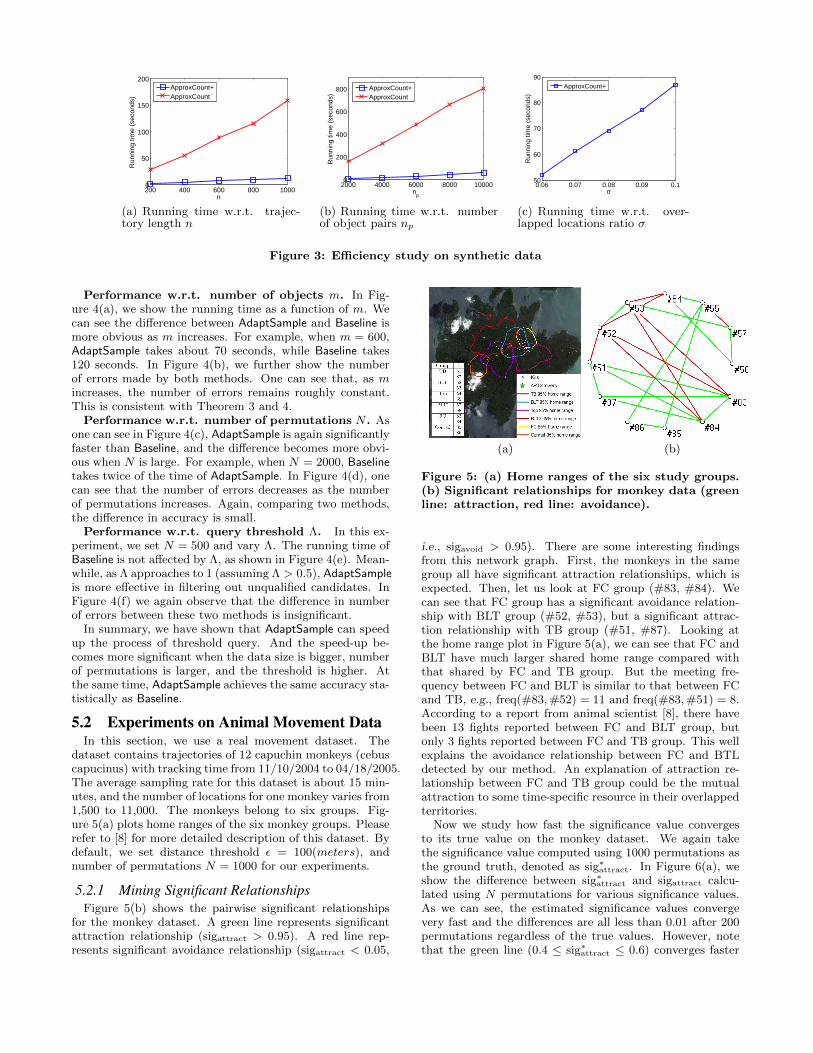
5.2 Experiments on Animal Movement DataIn this section, we use a real movement dataset. The

dataset contains trajectories of 12 capuchin monkeys (cebuscapucinus) with tracking time from 11/10/2004 to 04/18/2005.The average sampling rate for this dataset is about 15 min-utes, and the number of locations for one monkey varies from1,500 to 11,000. The monkeys belong to six groups. Fig-ure 5(a) plots home ranges of the six monkey groups. Pleaserefer to [8] for more detailed description of this dataset. Bydefault, we set distance threshold ε = 100(meters), andnumber of permutations N = 1000 for our experiments.

5.2.1 Mining Significant RelationshipsFigure 5(b) shows the pairwise significant relationships

for the monkey dataset. A green line represents significantattraction relationship (sigattract > 0.95). A red line rep-resents significant avoidance relationship (sigattract < 0.05,

(a) (b)

Figure 5: (a) Home ranges of the six study groups.(b) Significant relationships for monkey data (greenline: attraction, red line: avoidance).

i.e., sigavoid > 0.95). There are some interesting findingsfrom this network graph. First, the monkeys in the samegroup all have significant attraction relationships, which isexpected. Then, let us look at FC group (#83, #84). Wecan see that FC group has a significant avoidance relation-ship with BLT group (#52, #53), but a significant attrac-tion relationship with TB group (#51, #87). Looking atthe home range plot in Figure 5(a), we can see that FC andBLT have much larger shared home range compared withthat shared by FC and TB group. But the meeting fre-quency between FC and BLT is similar to that between FCand TB, e.g., freq(#83,#52) = 11 and freq(#83,#51) = 8.According to a report from animal scientist [8], there havebeen 13 fights reported between FC and BLT group, butonly 3 fights reported between FC and TB group. This wellexplains the avoidance relationship between FC and BTLdetected by our method. An explanation of attraction re-lationship between FC and TB group could be the mutualattraction to some time-specific resource in their overlappedterritories.

Now we study how fast the significance value convergesto its true value on the monkey dataset. We again takethe significance value computed using 1000 permutations asthe ground truth, denoted as sig∗attract. In Figure 6(a), weshow the difference between sig∗attract and sigattract calcu-lated using N permutations for various significance values.As we can see, the estimated significance values convergevery fast and the differences are all less than 0.01 after 200permutations regardless of the true values. However, notethat the green line (0.4 ≤ sig∗attract ≤ 0.6) converges faster

0 200 400 600 800 10000

0.01

0.02

0.03

0.04

0.05

N

|sig

attr

act −

sig

* attr

act|

≥ 0.9

≥ 0.4 and ≤ 0.6≤ 0.1

sig*attract

0 0.1 0.2 0.3 0.4 0.5 0.6 0.7 0.8 0.9 10

10

20

30

Num

ber

of p

airs

Sig*attract

(a) (b)

Figure 6: (a) Convergence rate of significance val-ues. (b) Histogram of significance values.

0 500 1000 1500 2000 2500

0

0.2

0.4

0.6

0.8

1

Average Distance (m)

Sig

attr

act

(a)

0 1 10 100 1000

0

0.2

0.4

0.6

0.8

1

Meeting Frequency

Sig

attr

act

(b)

Figure 7: Comparison with traditional measures

than the blue line (sig∗attract ≤ 0.1). This is in contrast tothe synthetic data case and Lemma 3, which suggest thatwhen sig∗attract approaches to 0 or 1, less number of per-mutations are needed to achieve the ε-approximation. Tounderstand this, we show the histogram of number of objectpairs w.r.t. to different significant values in Figure 6(b). Wefind that among the pairs whose sig∗attract values are in therange of [0.4, 0.6], there are 15 pairs which do not have anyoverlapped location in their trajectories (i.e., |R′| = 0). Forthose pairs, the estimated significance values converge to ex-actly 0.5 in one iteration, which greatly affects the averageconvergence rate for pairs in this group.

5.2.2 Comparing Significance Value with TraditionalMeasures

As we discussed before, previous work [30, 29, 6, 5] of-ten use (1) the Euclidean distance or its variants and (2)the meeting frequency to measure the relationship betweenmoving objects. Their assumption is that smaller Euclideandistance or larger meeting frequency indicates stronger at-traction relationship. We now demonstrate why this as-sumption is not necessarily true.

In Figure 7(a), we plot the significance value and the av-erage Euclidean distance for each pair of monkeys. We cansee that, if the average distance between two monkeys islarger than 1km, they usually have independent relation-ship (sigattract close to 0.5). This often occurs when twomonkeys have their own territories and their trajectories donot overlap. Meanwhile, when the average distance is lessthan 0.5km, the pair is very likely to have attraction re-lationship. However, when the average distance is in themiddle range of 0.5km-1km, the relationship can either beattraction, independent or avoidance. As a result, by us-ing the average distance, one cannot correctly identify therelationship in these cases.

Similarly, in Figure 7(b), we show that meeting frequencyis also not a good measure for attraction and avoidance re-

1002003004005000

500

1000

1500

2000

2500

3000

Distance threshold (meters)

Run

ning

tim

e(m

s)

ApproxCount+ApproxCount

(a)

1002003004005000

0.1

0.2

0.3

0.4

0.5

Distance threshold (meters)

Rat

io o

f ove

rlapp

ed lo

catio

ns

(b)

Figure 8: Efficiency study on synthetic data

lationships. As one can see, if the meeting frequency is high(> 20), two monkeys are very likely to have attraction re-lationship. However, when the frequency is in the middlerange from 1 to 20, the relationships can either be attrac-tion, independent or avoidance. Further, if two monkeyshave zero meeting frequency, they could either be indepen-dent or having an avoidance relationship.

5.2.3 Efficiency of Computing Significance ValueNext, we verify the effectiveness of the pruning rules we

developed in Section 3.3 on the monkey dataset. Figure 8(a)plots the running time of our methods ApproxCount andApproxCount+. We can see that ApproxCount+ is muchfaster than ApproxCount. For example, when the distancethreshold d = 100(meters), ApproxCount spends about 2200milliseconds to compute the significance value. On the otherhand, ApproxCount+ only takes 700 milliseconds to finish.To understand why this is the case, in Figure 8(b) we plotthe average ratio of overlapped locations between monkeypairs as a function of the distance threshold d. As one cansee, the ratio is typically very small. For example, whend = 100, that number of overlapped locations (i.e., |R′|) isonly 20% of the total number of points in R (i.e., n). Inaddition, as the distance threshold decreases, |R′| becomessmaller, and therefore Pruning I is more effective.

5.2.4 Efficiency of Threshold QueryLastly, we demonstrate that AdaptSample method can speed

up the threshold query processing without sacrificing the ac-curacy on the monkey dataset. In this experiment, we useone monkey as the query object and retrieve all the othermonkeys having significant values sigattract above thresholdΛ. We repeat the process for every monkey in the datasetand record the total time in Figure 9 w.r.t. the threshold Λ.

0.1 0.2 0.3 0.4 0.5 0.6 0.7 0.8 0.90

2

4

6

8

Λ

Run

ning

tim

e (s

econ

ds)

AdaptSampleBaseline

Figure 9: Threshold query on monkey data set

We can see that AdaptSample is significantly faster thanBaseline. For example, with Λ < 0.7, AdaptSample takes lessthan 1 second to process the threshold query, while Baseline

takes about 5.5 seconds. Note that, however, as Λ increasesfrom 0.5 to 0.9, the computation time for AdaptSample alsoincreases, which contradicts the result on synthetic dataset.The reason is that for the monkey dataset, the true signifi-cance values are not uniformly distributed in [0, 1], as shownin Figure 6(b). In particular, there is a large number of pairswith significance values in [0.9, 1], compared to the numberof pairs with significance values in [0.5, 0.9]. So AdaptSampletakes more iterations to process these pairs for bigger Λ.

In terms of accuracy, both methods retrieve identical ob-jects for all threshold queries, except when Λ = 0.1 and0.3,AdaptSample has 2 and 1 false positives, respectively.

5.3 Experiment on Human Movement DataIn this section, we use Reality Mining dataset (http://

reality.media.mit.edu) to evaluate the effectiveness andefficiency of our method on human movements. The datasetcontains movement data of 95 persons. A person’s move-ment data includes a sequence of timestamps and the corre-sponding cell tower IDs.

We use friendship survey, affiliation and group informa-tion as the ground truth in this experiment. Pairs havingcertain relationship (i.e., being friends, having the same af-filiation, or being in the same group) are denoted as 1 (apositive pair), and 0 otherwise (a negative pair). Out ofthe 4465 pairs in total, there are 68 friend pairs, 74 pairswho are in the same group, and 670 pairs that have sameaffiliation.

Group Affiliation FriendSignificance Value 0.6221 0.6538 0.7001Meeting Frequency 0.3104 0.3371 0.5053

Dynamic Time Warping 0.1967 0.2627 0.5576

Table 1: Cosine similarity score with ground truth

We use cosine similarity to compute the correlation be-tween ground truth and different measures including the sig-nificance value, meeting frequency, and dynamic time warp-ing distance. The number of permutations N is set to 1000for our method. Since the number of negative pairs is muchmore than that of positive ones, we sample the negativepairs to make the number balanced and report the aver-age cosine similarity over 1000 sampling trials in Table 1.As one can see, the cosine similarity scores between signifi-cance value and ground truth are always above 0.62, and areconsistently higher than the scores for meeting frequency ordynamic time warping.

The time complexities for calculating the meeting fre-quency, dynamic time warping and significance value for onepair are O(n), O(n2), and O(N · n), respectively. To com-pute the values for all pairs, it takes 1 second for meetingfrequency and 153 seconds for dynamic time warping. Therunning time for computing the significance values is 118seconds with pruning, and 233 seconds without pruning. Itworths noting that persons tracked in this dataset are allfaculties, staffs, and students at MIT. So they share signif-icant amount of overlapped locations in their movements.But our pruning techniques are still effective in this case.

6. RELATED WORKIn data mining literature, the problem of mining moving

object clusters, which aims to detect attraction relationships

among moving objects, has been extensively studied. Gener-ally speaking, a moving object cluster is “a set of objets thatmove together”. In particular, several measures have beenproposed to measure the similarity between trajectories, in-cluding the Euclidean Distance, Dynamic Time Warping(DTW) [30], Longest Common Subsequences (LCSS) [29],Edit Distance on Real sequence (EDR) [6], and Edit dis-tance with Real Penalty (ERP) [5]. The intuition behindthese measures is that, the more similar two trajectories are,the closer their relationship is. An alternative approach isto count the number of timestamps at which a set of objectsare located together. If the objects are frequently co-located,they form a cluster. Representative methods include movingcluster [17], flock [20, 12, 11, 1], convoy [16], swarm [21], andgathering pattern [31]. However, all the methods above donot consider the background model of the moving objects.Instead, they measure the degree of relationship based onthe similarity of trajectories or co-location frequencies. Aswe have previously shown, such measures are not necessarilyvalid for mining significant relationships.

Methods have also been proposed to characterize the tem-poral patterns in order to detect semantic relationships.Miklas et al. [24] find that “friends meet more regularlyand for longer duration whereas the strangers meet sporad-ically” and Eagle et al. [10] shows that friend demonstratesdistinctive temporal and spatial patterns. Then, temporaland spatial features are extracted to build the semantic re-lationship classifier in a supervised framework [7, 23]. Butin this paper we only focus on unsupervised methods.

In this paper, we use permutation test to calculate thesignificance values. The permutation test, also known asrandomization test or shuffle test, is a standard statisticalapproach, and has been applied to measure the significantcorrelation on social network [2, 3, 19], graph [13], and timeseries [4, 18]. The significance values of avoidance and at-traction relationships we define in this paper have rigorousstatistical semantics. However, computing the exact signifi-cance values is proved to be #P-hard. So we employ MonteCarlo sampling methods to compute the significance valuesand process the threshold queries approximately. Similarideas can be found in other areas of uncertain databases,such as the works on query evaluation in uncertain databases[27, 14, 15]. In particular, [27] evaluate the top-k querieswhich output tuples satisfying a query and with the top-khighest probabilities. A Monte Carlo sampling algorithmis used to compute the probabilities approximately and alower-higher bound shrinking scheme is developed to processtop-k queries efficiently. Although sharing some similarities,techniques in our work and the works on query evaluation inuncertain database cannot be applied interchangeably. Themajor reason is that uncertainty in our work arises from thestatistic model for defining significance, while uncertainty inthose works arises from data itself, not to mention the dif-ferences on the formulations of “probabilities” and “queries”for addressing different application interests.

7. DISCUSSIONIn this section, we discuss two interesting extensions of

our work. First, our current permutation method may gen-erate “impossible” trajectories. For example, two consecu-tive points in a randomized trajectory might be too far awayfor the object to travel within a time unit. It is thereforedesirable for our method to preserve certain spatiotemporal

properties in the trajectories while conducting the permuta-tion test. Such property could be the distance constraint onany two consecutive points, or some landscape constraintsinduced by a river, a mountain, or the road network. Theproperty can also come from certain known trajectory pat-terns of the moving objects, such as daily periodic patternsor seasonal migration patterns [22].

Second, in our current framework, we simply count themeeting frequency without considering the semantics in themeeting events. For example, meeting for 10 consecutivehours and meeting for 1 hour each day for 10 days obvi-ously carry different semantic meanings and therefore couldindicate different types of relationships. Also, some placesare visited more frequently in general, such as a public parkin down town, whereas locations like a private property arevisited much less frequently. Meeting events at differentlocations also carry different semantics. In the future, weplan to use the weighted meeting frequency to incorporatethe semantics into the relationship detection framework.

8. CONCLUSIONIn this paper, we propose a unified framework to detect

significant attraction and avoidance relationships in move-ment data. The idea of our method is that, in order to minesignificant relationships, one needs to look into the back-ground model of the movement data. Based on this idea,we propose to use permutation test to evaluate the signif-icance value of the relationships. Two pruning techniquesare proposed to speed up the permutation test. In addition,we discuss how to answer threshold queries for movementdatabase and retrieve all the objects having significant rela-tionships with the querying object. An early-stop strategyis employed for efficient query processing.

9. REFERENCES[1] G. Al-Naymat, S. Chawla, and J. Gudmundsson.

Dimensionality reduction for long duration andcomplex spatio-temporal queries. In SAC’07.

[2] A. Anagnostopoulos, R. Kumar, and M. Mahdian.Influence and correlation in social networks. InKDD’08.

[3] S. Aral, L. Muchnik, and A. Sundararajan.Distinguishing influence-based contagion fromhomophily-driven diffusion in dynamic networks.PNAS’09.

[4] N. Castro and P. J. Azevedo. Time series motifsstatistical significance. In ICDM’11.

[5] L. Chen and R. T. Ng. On the marriage of lp-normsand edit distance. In VLDB’04.

[6] L. Chen, M. T. Ozsu, and V. Oria. Robust and fastsimilarity search for moving object trajectories. InSIGMOD’05.

[7] J. Cranshaw, E. Toch, J. I. Hong, A. Kittur, andN. Sadeh. Bridging the gap between physical locationand online social networks. In Ubicomp’10.

[8] M. Crofoot, I. Gilby, M. Wikelski, and R. Kays.Interaction location outweighs the competitiveadvantage of numerical superiority in cebus capucinusintergroup contests. PNAS’08.

[9] C. P. Doncaster. Non-parametric estimates ofinteraction from radio-tracking data. Journal ofTheoretical Biology’90.

[10] N. Eagle, A. Pentland, and D. Lazer. Inferringfriendship network structure by using mobile phonedata. In PNAS’09.

[11] J. Gudmundsson and M. van Kreveld. Computinglongest duration flocks in spatio-temporal data. InGIS’06.

[12] J. Gudmundsson, M. J. van Kreveld, andB. Speckmann. Efficient detection of motion patternsin spatio-temporal data sets. In GIS’04.

[13] S. Hanhijarvi, G. C. Garriga, and K. Puolamaki.Randomization techniques for graphs. In SDM’09.

[14] M. Hua, J. Pei, W. Zhang, and X. Lin. Rankingqueries on uncertain data: a probabilistic thresholdapproach. In SIGMOD’08.

[15] R. Jampani, F. Xu, M. Wu, L. L. Perez, C. M.Jermaine, and P. J. Haas. Mcdb: a monte carloapproach to managing uncertain data. In SIGMOD’08.

[16] H. Jeung, M. L. Yiu, X. Zhou, C. S. Jensen, and H. T.Shen. Discovery of convoys in trajectory databases. InVLDB’08.

[17] P. Kalnis, N. Mamoulis, and S. Bakiras. Ondiscovering moving clusters in spatio-temporal data.In SSTD’05.

[18] J. Kawale, S. Chatterjee, D. Ormsby, K. Steinhaeuser,S. Liess, and V. Kumar. Testing the significance ofspatio-temporal teleconnection patterns. In KDD’12.

[19] T. La Fond and J. Neville. Randomization tests fordistinguishing social influence and homophily effects.In WWW’10.

[20] P. Laube and S. Imfeld. Analyzing relative motionwithin groups of trackable moving point objects. InGIS’02.

[21] Z. Li, B. Ding, J. Han, and R. Kays. Swarm: Miningrelaxed temporal moving object clusters. In VLDB’10.

[22] Z. Li, B. Ding, J. Han, R. Kays, and P. Nye. Miningperiodic behaviors for moving objects. In KDD’10.

[23] Z. Li, C. X. Lin, B. Ding, and J. Han. Miningsignificant time intervals for relationship detection. InSSTD’11.

[24] A. G. Miklas, K. K. Gollu, K. K. W. Chan, S. Saroiu,P. K. Gummadi, and E. de Lara. Exploiting socialinteractions in mobile systems. In Ubicomp’07.

[25] R. Motwani and P. Raghavan. RandomizedAlgorithms. Cambridge University Press, 1995.

[26] E. W. Noreen. Computer intensive methods for testinghypotheses. Journal of Theoretical Biology, 1989.

[27] C. Re, N. N. Dalvi, and D. Suciu. Efficient top-kquery evaluation on probabilistic data. In ICDE’07.

[28] L. G. Valiant. The complexity of computing thepermanent. Theor. Comput. Sci., 8, 1979.

[29] M. Vlachos, D. Gunopulos, and G. Kollios.Discovering similar multidimensional trajectories. InICDE’02.

[30] B.-K. Yi, H. V. Jagadish, and C. Faloutsos. Efficientretrieval of similar time sequences under time warping.In ICDE’98.

[31] K. Zheng, Y. Zheng, N. J. Yuan, and S. Shang. Ondiscovery of gathering patterns from trajectories. InICDE’13.