Louisiana State UniversityLSU Digital Commons

LSU Historical Dissertations and Theses Graduate School

1971

Atomic Systems With a Closed Core Plus TwoElectrons.Albert Ai-chun FungLouisiana State University and Agricultural & Mechanical College

Follow this and additional works at: https://digitalcommons.lsu.edu/gradschool_disstheses

This Dissertation is brought to you for free and open access by the Graduate School at LSU Digital Commons. It has been accepted for inclusion inLSU Historical Dissertations and Theses by an authorized administrator of LSU Digital Commons. For more information, please contactgradetd@lsu.edu.

Recommended CitationFung, Albert Ai-chun, "Atomic Systems With a Closed Core Plus Two Electrons." (1971). LSU Historical Dissertations and Theses.2051.https://digitalcommons.lsu.edu/gradschool_disstheses/2051

72-31187FUNG , Albert Ai-Chun, 1917-

ATOMIC SYSTEMS WITH A CLOSED CORE PLUS TWO ELECTRONS.

The Louisiana State University and Agricultural and Mechanical College, Ph.D., 1971 Physics, atomic

University Microfilms, A XEROX Company, Ann Arbor, Michigan

THIS DISSERTATION HAS BEEN MICROFILMED EXACTLY AS RECEIVED

ATOMIC SYSTEMS WITH A CLOSED CORE PLUS TWO ELECTRONS

A Dissertation

Submitted to the Graduate Faculty of the Louisiana State University and

Agricultural and Mechanical College in partial fulfillment of the requirements for the degree of

Doctor of Philosophyin

The Department of Physics and Astronomy

byAlbert Ai-Chun Fung

M. S., Saint Louis University, 1959 August 1971

PLEASE NOTE:

Some Pages have i n d i s t i n c t p r i n t . Fi lmed as rece ived.

U N I V E R S I T Y M I C R O F I L M S

FEFE AND OUR CHILDREN

ACKNOWLEDGEMENTS

The author wishes to express his gratitude to Professor John J. Matese for his very patient guidance throughout the course of this work.

Thanks are due to Drs. R. W. LaBahn and R. J. W.Henry for helpful discussions and comments. The author is indebted to the LSU Computer Research Center for making available the needed computational facilities.

Thanks are also due to Martha Prather for careful typing of the manuscript.

Financial assistance received from the "Dr. Charles E. Coates Memorial Fund of the LSU Foundation” for the publication of this work is also acknowledged.

ii

TABLE OF CONTENTSPage

Acknowledgements iiList of Tables vList of Figures viAbstract viiPart I Multiconfiguration Hartree-Fock

Description of Systems with a Closed Core Plus Two Electrons

1-1 Introduction 11-2 Multiconfiguration Hartree-Fock

Calculation of Energy 6A. Single Particle Orbitals 6B. The N-l Electron System 8C. The N Electron System 10

1-3 Detachment Potentials of Be, Li and Na 22A. The Ionization Potential of Be 22B. The Electron Affinity of Li 24C. The Electron Affinity of Na 29

1-4 Autoionization States of the e -Li ande -Na Systems 3 8

A. Theory of the Autoionization States 38B. Autoionization States of e -Li and

e~-Na Systems 441-5 Conclusions 47

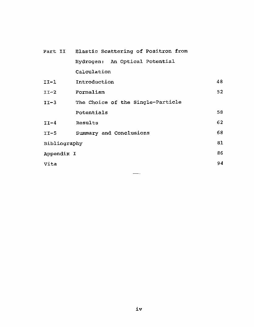
Part II Elastic Scattering of Positron fromHydrogen: An Optical PotentialCalculation

II-l Introduction 48II-2 Formalism 52II-3 The Choice of the Single-Particle

Potentials 58II-4 Results 62II-5 Summary and Conclusions 68Bibliography 81Appendix I 86Vita 94

iv

LIST OP TABLES

Table PageI. Glockler's Extrapolation Formula 2

II. Parameters of Basis Functions for Be+ 2 5III. Single Particle Eigenvalues in the V

Approximation for Be+, Li and Na 27IV. Parameters of Basis Functions for Li 30V. Convergence of the Electron Affinity

of Li 32VI. Polarizability of Li 33VII. Parameters of Basis Functions for Na 35VIII. Polarizability of Na 38

IX. Contributions to the second-order S-wavephase shift for Positron-HydrogenScattering 71

X. Third-order Ratios for K =.3 72oXI. Coefficients of Enhancement, Ce 73

XII. Positron-Hydrogen Phase Shifts 74

v

LIST OF FIGURES

Figures1

2

3

4

PagePoles and branch cuts in the singlechannel and coupled channel S-matrix 76Hartree-Fock energy levels for Li andthe multiconfiguration Hartree-Fockground state and metastable excited statesof Li 77Hartree-Fock energy levels for Na andthe multiconfiguration Hartree-Fockground state and metastable excited statesof Na~ 78Contributing diagrams to <KC|V |Ko>through third order 79S-wave positron-hydrogen phase shifts inradians. <Ss=Schwartz results, 6t=zero-

f 2)order results, '=second-order results. H=Hartree single-particle potential,H+B=Hartree plus Bethe single-particle potential 80

vi

ABSTRACT

This dissertation is divided into two parts. Part I consists of the formulation of a simplified method of superposition of configurations of Weiss for the calcula­tion of detachment potentials for systems with two electrons outside a closed core. The simplification does not impair the accuracy of the results. For the detach­ment of potentials of Be, Li- and Na~ all agree with Weiss to within 0.01 eV. It has the further advantage of the ease of constructing projection operators used in deter­mining autoionization states for e”-alkali atom systems, similar to the method proposed by Hahn, O'Malley andSpruch. For Li three autoionization states have been

2 2 found below the Is 3s level and four below the Is 3plevel. Only one autoionization state is found for Na.

Part II deals with an optical potential method for the calculation of the elastic scattering of positron from hydrogen atom. The single-particle states of the electron are chosen to be the hydrogenic solutions while the positron states are obtained by using a model polari­zation potential. Various models are investigated and a choice is made which effectively maximizes the calculated phase shifts through second-order in the perturbation expansion of the optical potential. Phase shifts thus obtained yield approximately 67%-80% of the difference between the static Hartree results and the variational

vii

results of Schwartz.

VJLZ1

PART I

MULTICONFIGURATION HARTREE-FOCK DESCRIPTION SYSTEMS WITH A CLOSED CORE PLUS TWO ELECTRONS

1-1. INTRODUCTION

The electron affinity (EA) of atoms is of interestto both physicists and chemists. For the case of alkaliatoms the EA can generally be computed more accuratelythan can be determined experimentally. Nonetheless suchcalculations are difficult because the EA is the smalldifference between two comparatively large numbers, theatom energy Eq and the ion energy E_. An accurate directcalculation of the EA can only be obtained if Eq and E_are computed with a high degree of precision or if Eq andE_ are known to be computed with the same absolute error.

Because of the computational difficulty involved inobtaining accurate values for the total energy of systemsof more than two electrons, extrapolation procedures havebeen developed which utilize precise experimental valuesfor the total energy of atoms and positive ions in theisoelectronic sequence. The first class of approximationsfits the experimentally determined ionization potentialsof the isoelectronic sequence to an analytic function ofZ, the nuclear charge, and extrapolates to find the detach-

2-5ment potential of the lowest member of the sequence.2Glockler was the first to use an extrapolation

formula to calculate the ionization potential (IP). Hesuggested, in 1934, the simple parabolic relation of

2 2 IP(Z) = (aZ - bz + c)/n , in which a, b, c, and n areparameters to be obtained from experimental values of

2

TABLE I: GLOCKLER’S EXTRAPOLATION FORMULA

2Shell Number of a b c a/nElectrons

K 1 13.,54 — — 13. 542 13., 54 16.87 4.06

L 3 3.,43 11.25 8.25 3.394 3.,43 15.10 14.77

IP(Z) = 2(aZ - bZ + c) /n2 (eV)

Sample calculations:

EA(H) = (13.54 x l2 - 16.87 x 1 + 4.06)/l = 0.73 eV.

IP(He) = (13.54 x 22 - 16.87 x 2 + 4.06)/l = 24.48 eV.

EA(Li) = (3.43 x 32 - 15.10 x 3 + 14.77)x 3.39/3.43 = 0.34 eV.

IP(Be) = (3.43 x 42 - 15.10 x 4 + 14.77)x 3.39/3.43 = 9.25 eV.

3

members of the iso-electronic sequence. Table I gives the values of the parameters obtained from experimental data available to him at that time and some calculated values of EA and IP.

gJohnson and Rohrlich proposed another formula which used five or more parameters. Although much newer (1959) experimental data were available, their success with different elements was very widely varied, because the parameters were very sensitive to small errors in the experimental IP's of the positive ions.

Typically the estimates of the EA obtained by theseextrapolation methods differ substantially depending uponthe extrapolation formula used and the experimental dataavailable. For Li, values ranging from 0.34 eV to 0.82 eV

1-3have been found.7 8A second class of approximations ' uses a consistent

computational scheme to calculate the total energy of the members of the iso-electronic sequence for N and N-l electron atoms and positive ions. A sequence of errors is then obtained by comparison with experiment and extra­polation of these errors is then used to estimate the EA. Because of the uncertainty in the extrapolation this approach is reliable only if the sequence of errors is sufficiently small and sufficiently smooth.

9Weiss has used a method of superposition of config­urations (SOC) to calculate the detachment potentials for

4

alkali ions and other elements. The method consists of writing a trial function for the N electron system as a linear superposition of terms which include the ground state Hartree-Fock function and a number of elaborately obtained virtual excited orbitals. The calculation of the energies is carried out in a manner which produces approximately the same error in both systems. His results agree very well with experimental values.

In the present work we calculate the energies of the N electron and the N-l electron systems in a similar

Qmanner as Weiss, but differing in the way of obtaining the virtual orbitals. The N-l electron system is described by a single configuration of orbitals contained from an analytic Hartree-Fock description using a self-consistent V ~ potential. The N electron system is described by a fixed core multiconfiguration Hartree-Fock wave function which uses the same orbitals obtained for the N-l electron system. Details of this formalism are contained in Sec. 1-2. Sec. 1-3 discusses an application of this formalism to obtain the electron detachment potential of Li and Na and the ionization potential of Be.

The existence of states of compound nuclei made up of an excited target nucleus and an incident nucleon has long been known to give rise to the strong resonances found in nucleon-nucleus elastic scattering. Similar phenomena existing in atoms such as the sharp maxima in optical

5

absorption and the resonant peaks of cross section in electron scattering can equally well be explained by the compound or autoionization states in atoms. In Sec. 1-4 we summarize the theory of the autoionization states of atoms then apply a projection formalism to compute these states for the e~-Li and e”-Na systems. Conclusions and a brief discussion are given in Sec. 1-5.

1-2. MULTICONFIGURATION HARTREE-FOCK CALCULATION OF ENERGY

The present formalism follows closely the analysis12 . . . of Salmona and Seaton which was applied originally to

scattering states of the electron-alkali atom system.Before discussing how configurations of the N-l and Nelectron systems are constructed we detail the methodused to obtain the analytic single particle statesutilized in the mixing.

A. Single-Particle OrbitalsThe single particle states used here are determined

by diagonalizing (self-consistently) the N-2 electronclosed shell Hartree-Fock Hamiltonian in the manner of

13Clementi.

<uj(d.)ih=°re(i)iuj:(i)> = e y6oo. « . , (i)

where E^ are single-particle energies and

uj(i) = uT (i) xCT(i)/

where y are the spin functions, the u^ are spin orbitals "-0 crwith spatial functions expanded in a set of Slater orbitals and spherical harmonics

6

7

uY(i) " \ m Y(i> £ byk V 1' * <3>

The lowest orbitals of the appropriate species are identi­fied as core orbitals and are determined in a self-con­sistent fashion. We label the core spin-orbitals bya^r i=l*,#N-2. The Hartree-Fock Hamiltonian is then given. 14by

hHFr0 = -V2 - + V-W , (4)

where

N-2V u^(i) = Z v(a. ,a.) vJ(i) , (5)

<* j=! 3 D

N-2W u^(i) = Z v(a.,u^)a.(i) , (6)

0 j=l J o J

and

v(aj,ak) = 2 |dr at(r) a}c(r)/|r-ri| . (7)

The choice of the vN-2 approximation for the single particle states is made for two reasons. First we desire a reasonable single configuration representation of the ground and excited states of the N-l electron system and these are best represented by the V11 approximation.

8

12Further, as shown by Salmona and Seaton, the formalism for describing the N electron system is materially sim­plified if the single particle orbitals diagonalize the core Hartree-Fock Hamiltonian.

The procedure used for choosing the Slater orbitals to be coupled in Eq. (3) is as follows. Although we self-consistently diagonalize in the approximationthe set of Slater orbitals which we use is that set ob­tained by dementi"^ in the approximation, augmentedwith additional Slater orbitals to better represent the lowest lying excited states of the valence electron. For those angular momentum species not included in the Clementi calculation we have simply chosen a reasonable basis set and in some cases have optimized parameters to obtain low lying excited valence states of these angular momentum species. In the present calculation only states with symmetry £=0,1,2 have been included.

B. The N-l Electron SystemThe ground state and lowest lying excited states of

the N-l electron system are represented by the single configuration

¥Y (N-1) = a1a2 * * ,aN_2 > <8>

where Dl_ , is the determinantal function N-l

9

D.N- l (ala 2 " -ai,_2 u^> =

/(N-l)! al ^ a2 ^ ^ - 2 ^ ua ^

ax(2)

a1 (N-l)------------- uJJ(N-l) (9)

Here the a. are the core spin-orbitals and u’Va. is the i o xsingle-particle valence spin-orbital (eg. for Li we have a1=ls+, a2 =ls+, and u^_+=2s+, 2p + , 3s+,-**) obtained as described above. The assumption that the excited states of the N-l electron system can be represented by single­particle excitations of the valence electron restricts the application to the lowest lying excited states. The wave function Eq. (8) is an eigenstate of orbital angularmomentum L=& , M=m , spin angular momentum S=^, M =cfT Y sand parity tt= (-1)L .

To simplify later calculations, the following ortho­normal conditions are imposed-.

10

ifj ” 1,2,■••N-2<a± 1 U(T = ° ' and all y,y't^ra*

<u^ * IuY> = 6 .6 . ,a* 1 (? yy era' *

Since adding a multiple of one column to another in a determinant does not change the value of the determinant, the above conditions do not change the wave functions.

C. The N Electron SystemMe describe the N electron system by a fixed closed

core of N-2 electrons with the multiconfiguration mixing of states of the valence and binding electrons

Y r (N ) = N Z E C t V s S f a - a O ) C (& - & - L ;m itu M )YCT x z j. z

x u l O * (10)

Here N is the normalization constant and y is the valencerstate. The states chosen to be coupled are such that V

is an eigenstate of L, S, M, M =0, and tt=(-1)L . We im- pose <a |<|> >=*0 to simplify computation. No other con­ditions are imposed on u0 or <t>0 , thus, in general, <uJ|*J >^0. For singlet states, this allows the valence and binding electrons to have the same space orbital.

11

The non-relativistic Hamiltonian is given by

N NH(N) = E f (i) + E g(if j) (11)

i=l i>j=l

where

f (i) = -V2 (i) - — ri

and

(12)

g(irj) = 2/rij , (13)

V T*The functional <y |H-E|4f > is then constructed and is simplified in the following manner.

We first consider the matrix elements of < d " ^ ° J F J i y ° > where the D's have the form of Eq. (10) and F is single­particle, two-particle, or constant multiplier operators.

15Condon and Shortley have discussed a method of evaluating integrals involving products of two determinantal functions in each of which all elements are mutually orthonormal. Because of the fact that, in general <u^ | , somemodifications of the method are necessary (see Appendix I). With this modified method, the following results are obtained. In order to express the results in a more general form, the orthonormality relation, <u^,|u^>=5 ,6 , , is not utilized at this stage.yy aa

12

(1) F = 1.

<DY,a’|F|DYa> = <Dy '°' jDY0>

= <uY !iuY ><4>Y , I j(|)Y >-<u y ! u y ><*Y , ,iuY > a ' 1 ct cr,|y-cr ^-a' 1 a •

(14)

N(2) F = E f (i) .

i=l

<DY 'a |FjDYa>

= E <a± |f |ai>{<<))Y^( |<j)Ya><uY! iuY> i=l

“ ^I'a* lu^><uji\*la>} + lf l11

+ < * 1 ^ lf U l a><uj!|uj> - < ^ , |uy><uy; |f |(f)Ya>

- <4>^, |f |uY ><uY ! |<{)Y a > . (15)

N ,. . v(3) F = E

i> j=l

<DY,°'|F|DYa>

N-2E {<a±a.|g|a.a.> - <a.a.|g|a.a±>}

i>j=l j j j j

13

+ <uYV | g | u V > - <uY:<tY',|gUY uY> a ,Y- a iy i V - o a ' Y- a ' 1 y 1 Y- a a

+ { < 3 ^ , I g l a ^ x u ^ ! |uj>

+ O i u j l l g l a i ^ x ^ o ' ^ V

- <ai<J,Io> lglaiua><ua* i(Io>

- <aiu^lglai'l’I(,><'t'Io.No>

- <ai<l'Io1l9 l+-aai><uo ' |u^

- <aiuY!|g|uYai><l|’-o'l','-a>

+ <ai4'Io. lgl“Jai><u^ !♦!(,»

+ <a iuY ! I g U l ^ i X ^ I o ’ • (16>

Note that in performing the spin sums, restrictions must be imposed on the spins in order that the exchange terms do not vanish. For example, in Eg. (16), the last four terms yield, respectively,

14

a ' = a - - a . ,i '

o ' = a = a± r

a' = -a = - a ± ,

a 1 = -a = .

Therefore, only (N-2)/2 terms contribute in the sum over i (for example, if lsf contributes, then ls-f does not, etc.). To remind ourselves of this fact we shall denote such a sum by S'.

The relations

C (hhS; cr-crO) = ( - 1 ) S + ^ C (h%S; -crcrO)

and

2 C 2 (HhSja-aO) = 1 a

are used to perform the spin sums. We obtain the following equation in which the a^'s stand for spinless core orbitals.

2 C 0 - c f O ) C t ^ J s S r a ’ - a ' O ) < D Y ' a ' | H - E | D YCT>a a '

= <dy *|H-E|Dy >

15

= [<UY' j u ^ x ^ ’ |4jY> + (-l)s<uY' |*Y><0Y'|UY>3

N-2 N-2x [-E + Z <a.a.|g|a.a.> - Z'<a.a.|g|a•a±>

i>j J J i>j J JN-2 , ,

+ Z <a^[f[a^>] + <*Y j(|)T>{<uY |f|uY>

N-2 , N-2+ Z <a.uY |g|a.uY> -ZT <a. uY |gjuYa.>}J i <L ' __T J* *

+ <uY'|uY> {<<j>Y* |f |<j)Y> + Z <ai4>Y lg|ai(fiY>i

- Z> <a±(>Y ’ |g|(f,Ya;L>} + (-1) S{<<)>Y' | uY><uY' | f | <J>Y>

+ <uY |{j)Yx<|)Y |f|uY> + <uY (jjY jgj(J)YuY>

+ <uY | cf>Y> C Z < a ^ T I g I a±uY>

Z' <a.(j>Y |g|uYa.>] + <tf>Y |uY> i

N-2 , N-2 ,[ Z <a±uY |gja±4>Y> - Z,<aiuY [g|(|)Yai>]}

+ <uY (|>Y |gjuY<f>> • (17)

We now observe that the Hartree-Fock Hamiltonian defined by Eq. (4) and the energy for the alkali core are given by

16

N-2hjjp e (j)<Kj) = + S <ai (k) |g (k, j) | a± (k) >

N-2|iMj)> - 2 1 Jai (j) x a ^ k ) jg(k, j) | if> (j ) > / (4')

and

N-2E H F = ? < a i ( k ) l f ( k )

1

N-2+ 2 <a.(l)a.(2)|g(l,2)|a.(l)a (2)>

i> j -1 -*N-2

- 2r <a.(l)a.(2)|g(l,2)|a (l)ai (2)> . (18)i> j 3 3

Recalling Eq. (1),

<uY' ihSlreiuY> = v v.Y . (1'>

We have:

<dV'|H-E|dY> = - ( E - E ^ e-EY)|^>

+ <uY <}>T |g|uY<f>Y> + (—1)S {<u^ (j)Y |h^°re(l)

+ h ^ re(2) - (E-E^re) | ^ uY> + <uY ' ' | g | <f)Yu^>}J

(19)

17

In performing the sum over m, we define:

uY (r) = uY (r) Y« m (r) , (20)

<j>Y(r) = <(>Y(r) Ya (r) , (21)2 2

* V n1 2 > - 37TT I yxu‘; 2 > > <22>

sxa,2) = r*/r*+1 , (23)

_ Z c ^ l 12L 'Inlm 2M *Y X1m 1 r l* Y H-m_*r 2 ' •1 2 m, m 0 l i 2 2

(24)T “ 2

Then;

g(l,2) = 2 Z Sx(1,2) Px(«12) , (25)

<YL££JlJ<ni2 ) l1CLJ&1 £2 tfi1 2 )> = 6jl!£i 5 j t 2 A 2 *

£ <<ieLJLjfcJ*nl2 * lXL£1 a2 tfi2 1 ,> = (_1) 6 *1 * 2 6 jl2 £l '

(27)

<YLJl££j<ni2) lPx!YLA1Jl2 (fl12,> = fX f£i£2Al£2?L) > (28)

18

M 1UI A J + A ' - L<YLJl|A^fi1 2 ) lPllYL£1 Jl2 (n2 1 ) 51 = C“1>

x t (29)

where the angular factor f is given by Percival and X 6Seaton. We have:

- (E-E°°re-EY) + e2 s f U ^ S L ^ J - L )X X

. , S+JIt+JL-j-Lx <u^ <f> |S |u (j) > + (-1 )

V 1 Y ' i ^ 2 ^ 1^|Y aY Vi * M -V Vi Xx ^ A ^ . 6 A J A X < u * lh H F (1) + h H F {2)

x <uY 4>Y ! t 4>YuY>] } f (30)

where

-2W

Y Y* . {V V i V i <tT' l*T><uT' luY>S + A n+ A , - L

+ (-1) 1 6 a V 6sl V <(t>y , | u Y > < u Y 14>Y > > , 1 2 x'2x'i

(31)

h W = - + AL*!1L - + (V-W)core . (3dr r

If we choose arbitrary Slater orbitals as bases for an expansion of the radial wave functions, <f>Y, the ortho gonalization process to make <a^ | <f>Y > = 0 may be quite tedious. This process can be made unnecessary, however, if we simply express <f>v in terms of uY, Eq. (3) ,

4)V = Z C uY . (33)Y Yv

Thus we see one of the advantages of using the same single­particle states for both the N-l and N electron systems.It also eliminated the extra work of generating the virtual

9 vexcited orbitals as done by Weiss. Further, <}> can also be easily made orthogonal to Hartree-Fock representation of any of the lowest lying excited states of the N-l electron system obtained above by simply restricting the summations over y to exclude the state desired.

Using Eq. (33) and the orthonormality relation <uY |uY > = 6 , , (also note that +&--L=even), Eq. (30)can further be simplified:

20

x {Cbhf +V e v-e] S v 'v y'1

+ 2 E £ x ^ S' Y ' !!' \ i , *'Yllv i:L* <uY l s ^ l uYuV>X

+ 2(-l)S Z £x(Zy,J>v,J>v£,y;L) < u Y * UV ' | Sx | uVuY> } f X

(34)

and

W" 2 = z Z C C , , [ 6 , 6 . + (-l) S 6 , 6yv y ,v. YV y'v’ YY* vv* yv‘ vy’ *

(35)

We note that Eq. (34) takes this particularly simple form only if the single-particle states are obtained from Eq. (1). Eq. (34) can be written in the matrix form:

Z C [H -E S _] C_ = 0 , (36)ag a L a6 a6 0

where H and S are the Hamiltonian and overlap matrix elements on the basis of functions uY (l)f uv(2) of Eq. (3), and a-(y,v), 3=(y ,#v i). The variational principle gives:

I tHccfTE s a S 3 c 6 = 0 • (37)

21

Standard techniques are used to solve this matrix eigen­value problem.

We conclude this section by noting that the single configuration approximation for the (N-l) electron state has an energy

1-3. DETACHMENT POTENTIALS OF Be, Li AND Na

A. The Ionization Potential of BeAs a test of the present formalism we have considered

the ionization potential of Be, a quantity which has beendetermined quite accurately both experimentally andtheoretically. The single-particle states generated from

_| |_Eq. (1) diagonalize the Be Hartree-Fock Hamiltonian.The Slater basis functions of Eq. (3) take the form

nk " 1 _*kr f . (r) = N . r eyk yk

nk+ 0 , 5 kV = (2 Xk} /C(2nk)!r (38)

where N^k is a normalization factor and the parametersnk' ^k ^or a 9 -*-ven angular momentum species are listed inTable II. (Also included in Table II are coefficientsb^k of Eq. (3) for the two lowest states of each momentumspecies and the total energy obtained in this work as well

13as those of Clementi. ) We have used 10(8,5) orbitals for s(p,d) species. The energy eigenvalues, E^ of Eq. (1) are given in Table III. The eigenvector associated with the lowest energy s state is identified with the Is orbital and is treated self-consistently. We label theeigenstates of Eq. (1) by Is, 2s,..... 10s; 2p, 3p,***9p;3d, 4d,***7d in order of increasing energies. However we

22

23

note that only those states nil with n£4 can be consideredto be reasonable Hartree-Fock approximations to thehydrogen-like excited states of the valence electron.Although all eigenstates are localized some have energiesin the continuum. This is desirable because it is knownthat the mixing of continuum-like states is important to

17obtain good energies.2 2The Hartree-Fock energy for the Is 2s S configuration

of Be is found to be -28.55472 Ry. This is to be com-7pared with the essentially exact value of -28.64958 Ry.

Approximately 90% of this difference is due to the corre­lation energy between the Is electrons with the remainder

18due to the correlation between the 2 s and Is electrons.The essential feature of the present calculation is that one expects essentially the same error in the core corre­lation energy and the valence electron-core correlation energy when the "binding" electron is added to give an N electron system if the same single particle states are used for both the N-l and N electron systems.

The energy of the ground state of Be was computed using Eq. (34) with a mixing of 34 configurations for the outer two electrons which included

2 2 2 yv(S) = 2s r2s3s,••*2s8s;3s ;*«»3s8s;4s ;

2p^,•*•2p8p;3p^,••*3p8p;4p^;3d^,•••3d7d;4d^(39)

24

The energy computed in this manner was found to be-29.23665 Ry. Taking the difference between this value

+and the Hartree-Fock energy of Be computed here we obtainan ionization potential for Be of 0.68193 Ry. This is ingood agreement with the essentially exact value of 0.68524Ry. which is obtained by adding to the precise two-electron

19ion energy results of Pekeris the experimental ionization energiesrelativistically corrected. This suggests that our basic assumption of cancelling errors in the energies computed in the manner described above is well founded for systems with two electrons outside a closed core.

B. The Electron Affinity of LiThe procedure followed for computing the energies

of Li and Li” is precisely the same as above. Table IV gives the parameters of the Slater basis functions, eigen­values and eigenvectors of the two lowest lying states foreach momentum species as obtained by this work as well as

13those obtained by dementi. Eigenvalues for higherstates are given in Table III. The Hartree-Fock energy

2 2for the Is 2s S configuration of Li was found to be-14.86544 Ry. in good agreement with previous calcula-

13 20tions. ' The configurations listed in Eq. (39) were mixed and an energy of -14.91049 Ry. was obtained for Li . This corresponds to an electron affinity of 0.04505 Ry.

TABLE II; PARAMETERS OF BASIS FUNCTIONS FOR Be+

(A) &=0

nk xk

This-28,

Is-11.33418#

Work55472*

2 s-1.33213$

dementi ^-3

-28.55466*Is 2 s

-10.27718# -1.33228$

1 6.96969 0.05214 -0.00842 0.06476 -0.011891 4.80000 0.05085 -0.01315 - -1 3.49627 0.89650 -0.19691 0.94315 -0.211232 2.50092 0.01826 -0.15573 -0.00058 -0.151982 1.29671 -0.02095 0.51691 0.01560 0.530542 1.11089 0.01736 0.62066 0.01070 0.601182 0.60000 -0.00182 -0.00685 - -2 0.25000 0.00028 0.00068 - _

2 0.05000 -0.00003 -0.00006 - -2 0 . 0 0 1 0 0 0 . 0 0 0 0 0 0 . 0 0 0 0 0 — —

* Total energy, shown only in table for £=0.# Is single-particle energy.$ 2 s single-particle energy.

Note: The same format is used for the p- and d-states andfor Tables IV and VII.

25

TABLE IX: (CONTINUATION)

(B)

nk *k

2 p-1.03881

3p-0.45650

2 3.50000 0.02870 -0.070932 2.50000 -0.01573 0.347282 1.80000 0.00653 -0.969782 1 . 2 0 0 0 0 0.45272 2.800672 0.90000 0.62362 -6.124182 0.67000 -0.07981 4.388922 0 . 2 0 0 0 0 0.00154 0.038382 0 . 0 0 1 0 0 -0 . 0 0 0 0 0 -0 . 0 0 0 0 0

(C) 1=2

3d 4d

nk *k -0.44286 -0.22450

3 2.50000 0.02948 -0.096723 1.50000 -0.15729 0.523503 0.90000 0.65370 -1.763303 0.50000 0.51722 1.381913 0.15000 -0.02980 0.27624

26

TABLE III: SINGLE PARTICLE EIGENVALUES EYIN THE APPROXIMATION FOR Be+, Li AND Na

Be Ll. Na

Is -11.33418 -5.58472 -81.519442 s -1.33213 -0.39261 -6.147363s -0.53294 -0.14693 -0.363624s -0.27541 -0.07167 -0.140115s -0.08887 -0.03250 -0.057316 s -0 . 0 0 2 0 0 -0 . 0 0 1 0 0 0.088207s 0.12485 0.16567 1.66161Bs 3.37051 1.86378 8.937129s 19.87050 10.01469 36.20718

1 0 s 132.69202 62.97964 161.38448

2 p -1.03881 -0.25727 -3.594373p -0.45650 -0.11302 -0.218354p -0.24094 -0.06002 -0.100455p -0.03496 -0 . 0 0 1 0 0 0.003036p -0 . 0 0 2 0 0 0.03700 1.113347p 1.16730 0.60414 5.907558 p 5.57627 2.99675 21.209269P 25.47377 16.21537 79.89123

3d -0.44286 -0 . 1 1 1 1 2 -0.111334d -0.22450 -0.05175 -0.051455d -0.14269 0.01757 0.064376 d 0.74269 0.84610 1.288197d 6.20990 6.21842 7.20673

27

28

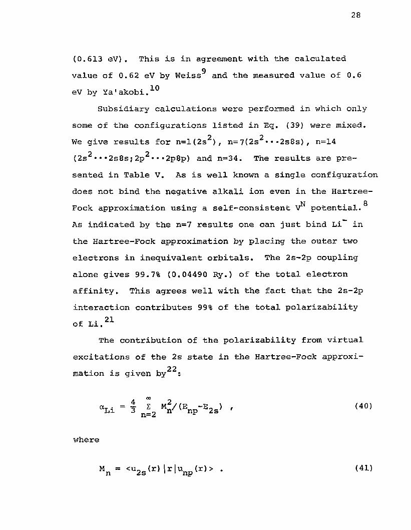
(0.613 eV). This is in agreement with the calculatedgvalue of 0.62 eV by Weiss and the measured value of 0.6

eV by Ya'akobi.^Subsidiary calculations were performed in which only

some of the configurations listed in Eq. (39) were mixed.2 2We give results for n=l(2s ), n=7(2s •■•2s8s)/ n=14

2 2(2s ***2s8s;2p ••■2p8p) and n=34. The results are pre­sented in Table V. As is well known a single configuration does not bind the negative alkali ion even in the Hartree- Fock approximation using a self-consistent V1 potential.®As indicated by the n=7 results one can just bind Li in the Hartree-Fock approximation by placing the outer two electrons in inequivalent orbitals. The 2s-2p coupling alone gives 99.7% (0.04490 Ry.) of the total electron affinity. This agrees well with the fact that the 2s-2p interaction contributes 99% of the total polarizability of Li . 2 1

The contribution of the polarizability from virtualexcitations of the 2s state in the Hartree-Fock approxi-

22mation xs gxven by :

a = i 2 M 2/ (E -E „ ) , (40)Lx 3 n_2 n np 2s

where

Mn = <u2s(rl M unp(r)> • (41)

29

The total polarizability of Li and the contributions from different states np are given in Table VI.

We have also investigated the Li system in the 3 S, 1 3 1 3' P, ' D states and find, as anticipated, that it does not bind. The configurations included 31 terms for P and 33 terms for D and are given below

yv (P) 2s2p,2s3p,••*2s8p;3s2p*•*3s8p;4s2p••• 4s4p;2p5s••*2p8s;3d2p*•*3d4p;4d2p»•-4d4p • (42)

yv(D) 2s3d,2s4d-•*2s6d;3s3d,••*3s6d;4s3d*•*4s6d;2p2p*•*2p8p;3p3p»••3p8p;4p4p;3d3d,••-3d6d;4d4d» * *4d6d . (43)

Upon request from A. K. Rajagopal, we investigated the possibility of the existence of bound states of a positron in a Li atom. The result was negative as we anticipated.

C. The Electron Affinity of NaFor Na we have proceeded in a manner similar to the

Be calculation. However we must now self-consistently solve for the Is, 2s and 2p orbitals in the core. We haveaugmented the Clementi Slater orbitals with only twoadditional orbitals of the s species and three additional

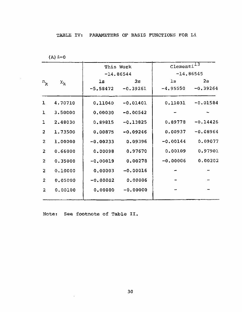
TABLE IV: PARAMETERS OF BASIS FUNCTIONS FOR Li

(A)H=Q

nk *k

This-14.

Is-5.58472

Work86544

2 s-0.39261

Clementi^ -14.86545

Is 2 s -4.95550 -0.39264

1 4.70710 0.11040 -0.01401 0.11031 -0.015841 3.50000 0.00030 -0.00542 - -

1 2.48030 0.89815 -0.13825 0.89778 -0.144262 1.73500 0.00875 -0.09246 0.00937 -0.089642 1 . 0 0 0 0 0 -0.00233 0.09396 -0.00144 0.090772 0.66000 0.00098 0.97670 0.00109 0.979012 0.35000 -0.00019 0.00278 -0.00006 0 . 0 0 2 0 2

2 0 . 1 0 0 0 0 0.00003 -0.00016 - -

2 0.05000 -0 . 0 0 0 0 2 0.00006 - -

2 0 . 0 0 1 0 0 0 . 0 0 0 0 0 -0 . 0 0 0 0 0 - —

Note: See footnote of Table II.

30

nk

22222222

nk

33333

TABLE IV: (CONTINUATION)

(B) S=1

2 pv, -0.25727

3.50000 0.004271.80000 0.018481 . 0 0 0 0 0 -0.010460.71109 0.106830.49782 0.915430.33300 -0.017190 . 1 0 0 0 0 0.000520 . 0 0 1 0 0 -0 . 0 0 0 0 0

(C) S=2

Xk

2.500001.200000.600000.333000.10000

3d■0.11112

0.00026-0.000210.001740.99885-0.00034

31

TABLE V: CONVERGENCE OF THE ELECTRON AFFINITY OF Li

n Electron Affinity (Ry.)

1 -.075357 .0065714 .0449034 .04505

32

TABLE VI: POLARIZABILITY OF Li

Coupling Polarizability Total

2 s-2 p 167.29693 167.296932s-3p 0.18928 167.486212s-4p 0.08811 167.574322s-5p 0 . 0 0 0 0 0 167.574322 s-6 p 0.91391 168.488232s-7p 0.47267 168.960892 s-8 p 0.01921 168.980102s-9p 0.00019 168.98029

Experimental value of the total polarizability is 148.5+13.5.21

33

34

orbitals of the p species. Therefore the low lying ex­cited valence states are not as well represented as they

+are for Be or Li. The Slater parameters and singleparticle energies are given in Tables VII and III. The

2 2 6 2Hartree-Fock energy for the Is 2s 2p 3s S configurationof Na was found to be -323.71749 Ry. which is to becompared with the value -323.71778 Ry. obtained bydementi^ using single particle orbitals of the V15 ^approximation. The mixing of 34 configurations (Eq. (39)with ns+(n+l)s, np-»-(n+l)p) yielded an energy of -323.75690Ry. for Na” from which we compute an electron affinity of0.03941 Ry. (0.536 eV). This is to be compared with the

gvalue of 0.54 eV of Weiss.The total poarizability of Na and the contributions

from different p-states are also calculated and are pre­sented in Table VIII.

TABLE VII: PARAMETERS OF BASIS FUNCTIONS FOR Na

(A) Jt=0

"k Xk Is-81.51944

This Work -323.71749

2 s-6.14736

3s-0.36362

Is-80.95698

dementi"*''*-323.71778

2 s-5.59404

3s-0.36422

1 1 1 . 0 0 0 0 0 0.96305 -0.23503 0.03505 0.96305 -0.23508 0.035323 12.36850 0.04218 -0.00375 0.00085 0.04219 -0.00373 0.000873 8.02540 0.01596 0.13140 -0,02214 0.01590 0.13129 -0.022373 5.70590 -0.00286 0.40151 -0.06238 -0.00281 0.40213 -0.062773 3.63100 0.00163 0.52747 -0.09330 0.00159 0.52699 -0.094213 2.15370 -0.00036 0.04775 0.00162 -0.00033 0.04726 0.002543 1.10810 0.00016 -0.00738 0.41288 0.00013 -0.00585 0.414863 0.70830 -0.00008 0.00323 0.63771 -0.00005 0.00217 0.636073 0.35000 0 . 0 0 0 0 2 -0.00066 0.00107 - - -3 0 . 1 0 0 0 0 -0 . 0 0 0 0 0 0.00009 0.00007 - - -

Note: See footnote of Table II.

TABLE VII: (CONTINUATION)

<B) S.=l

nk Xk

This2p

-3 .59437

Work3p

-0.21835

Clementi'*'3

2p 3p -3.03626 -

2 5.50000 0.47426 -0.04708 0.47360 -4 8.39370 0.03581 -0.00333 0.03555 -4 5.42060 0.27777 -0.02593 0.27825 -4 3.56460 0.32520 -0.02911 0.32310 -4 2.28330 0.06976 0.03483 0.07308 -4 1 . 0 0 0 0 0 -0.00253 0.56319 _ -

4 0.50000 0.00153 0.65161 -4 0.33300 -0.00078 -0.15675 - -

(C) 1=2

nk Xk3d

-0.111334d

-0.05145

3 3.20000 -0.00175 -0.003243 1.50000 -0.00236 0.013363 0.70000 -0.00512 -0.066813 0.33300 -0.99667 -0.272373 0 . 1 0 0 0 0 0.00103 1.03886

36

TABLE VXII: POLARIZABILITY OF Na

Coupling Polarizability Total

3s-3p 186.93607 186.936073s-4p 0.74289 187.678963s-5p 0.15197 187.830923s-6p 0.08467 187.915593s-7p 0.00015 187.915763s-8p 0.00028 187.916023s-9p 0 . 0 0 0 0 0 187.91602

Experimental value of the total polarizability is 145.1+13.5.21

37

1-4. AUTOIONIZATION STATES OF THE e -Li AND e -Na SYSTEMS

A. Theory of the Autoionization StatesIn this section we summarize the theory of the com­

pound atom or autoionization states, using the approach23developed by Feshbach, and applied to atomic systems by

several other authors. 4-26Consider an elastic scattering problem. Let q

represent the coordinates of the incident particle relative to the heavy nucleus of the target atom and let r represent the coordinates of the atomic electrons. The total

-AHamiltonian and total energy of the system, target atom plus incident particle, are denoted by H and E, respec­tively. The ground state of the target has a wave function

(r) and an energy E . e '-E-E is then the incident To o oparticle energy. The excited state wave functions and energies of the target are denoted by ^ (r) , ifj?(r)*»*, and E1, E2,**», respectively. By assumption, E lies below E^, or equivalently E' is smaller than E^-Eq, so that excitation is not energetically possible.

The regular solution of yT (r,q) ofJj

(H-E) ¥L (r,q) = 0 (44)

which satisfies the boundary condition that as

38

39

determines the phase shift nT to within a multiple of tt.§

0 is the angle between q and some fixed axis.23 24Following Feshbach and Hahn, O'Malley and Spruch,

we now introduce a pair of projection operators, P and Q, which operate in the space of the target particle co­ordinates. P is defined by

p = i v ^ o l ' <46>

that is, P projects onto the ground state of the target, while Q projects onto all of the excited states of the target, including the continuum states. Therefore, we have

P + Q = 1 . (47)

We can rewrite Eq. (44) as

(P+Q) (H-E) (p+Q)YL = 0. (48)

Since P and Q operate in orthogonal space, Eq. (48) can be rewritten into a pair of equations

P(H-E) (P+Q)fL = 0 , (49)

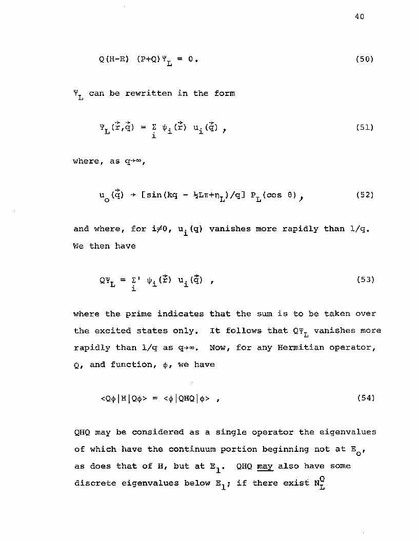
40

Q(H-E) (P+Q)¥l = 0, (50)

V can be rewritten in the form-L

yL (r,q) = 2 TjJiCr) u±(q) , (51)

where, as q**00,

u (q) -+• [sin(kq - JsLiT+nT)/q] PT (cos 6 ) . (52)O Jj J-i 7

and where, for i/0 , u^(q) vanishes more rapidly than 1 /q. We then have

QYt = 2' i|>. (r) u. (q) , (53)1

where the prime indicates that the sum is to be taken over the excited states only. It follows that Q1? vanishes more rapidly than 1/q as q-»“». Now, for any Hermitian operator,Q, and function, <J>, we have

<Q4» |H|Q<(» = <<f> |QHQ| <f>> , (54)

QHQ may be considered as a single operator the eigenvalues of which have the continuum portion beginning not at Eq, as does that of H, but at E^. QHQ may also have somediscrete eigenvalues below E^; if there exist N^

orthonormal states of total angular momentum L which satisfy

Q(H-E^n) Q$ £n= 0 , n=l,2,..-N° , (55)

with E^ <E^, the spectrum of Q(H-E)Q in the space of totalangular momentum L will include the discrete eigen-L»values, E^n~E, and the continuum bounded from below by the positive value of E^-E. The discrete states are the autoionization states below the level E^. If, for example, Eg<E<Eg, we redefine

2P = 2 | iK > <iK | , (56)

i= 0 1 1

and the autoionization states obtained will be those below the level of Eg. These states will appear just like ordinary bound states in the calculation.

To explain why the autoionization states are reso­nance states, it is convenient to use the properties of

27the coupled channel S-matrix. We consider a finite number of channels with two particles in each. The c oupled equations describing the radial motion of the scattering particles are:

42

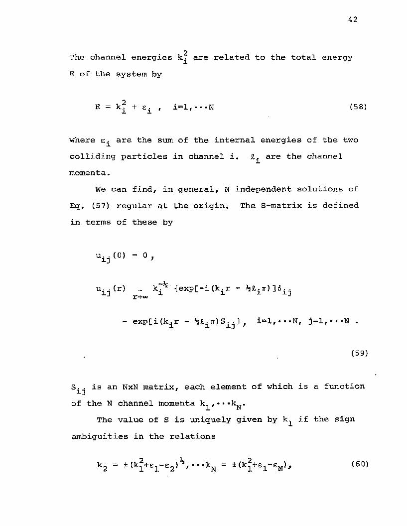
2The channel energies k^ are related to the total energy E of the system by

(58)

where are the sum of the internal energies of the two colliding particles in channel i. SL are the channel momenta.

We can find, in general, N independent solutions of Eq. (57) regular at the origin. The S-matrix is defined in terms of these by

S.. is an NxN matrix, each element of which is a function of the N channel momenta

The value of S is uniquely given by k^ if the sign ambiguities in the relations

u..(0 ) = 0 13

u . . (r) ~ kT3* {expOitK^r -

- exp[i(k.jr - } ; i=l, • • *N, j=l, • • *N

(59)

(60)

43

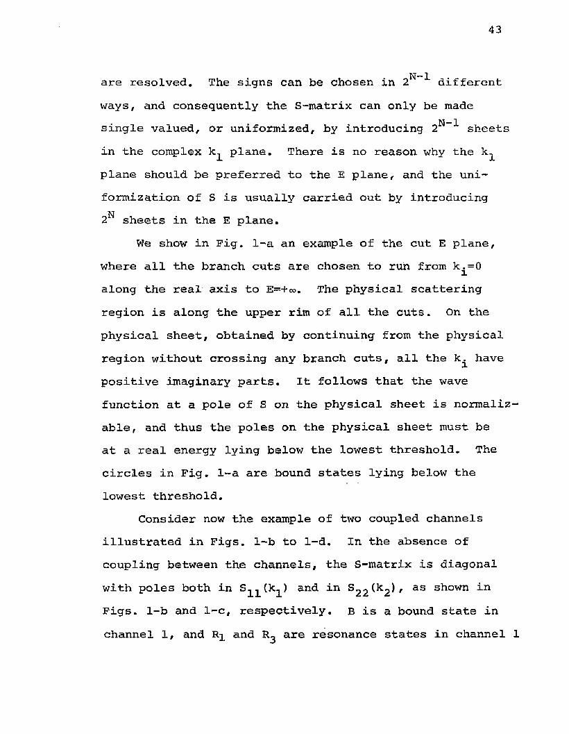
are resolved. The signs can be chosen in 2 differentways, and consequently the S-matrix can only be madesingle valued, or uniformized, by introducing 2 N ~ 1 sheetsin the complex k^ plane. There is no reason why the k^plane should be preferred to the E plane, and the uni-formization of S is usually carried out by introducing N2 sheets in the E plane.

We show in Fig. 1-a an example of the cut E plane, where all the branch cuts are chosen to run from k . = 0ialong the real axis to E=+ro. The physical scattering region is along the upper rim of all the cuts. On the physical sheet, obtained by continuing from the physical region without crossing any branch cuts, all the k^ have positive imaginary parts. It follows that the wave function at a pole of S on the physical sheet is normaliz­able, and thus the poles on the physical sheet must be at a real energy lying below the lowest threshold. The circles in Fig. 1-a are bound states lying below the lowest threshold.

Consider now the example of two coupled channels illustrated in Figs. 1-b to 1-d. In the absence of coupling between the channels, the S-matrix is diagonal with poles both in S-^(k^) and in 8 2 2 ( 2 ' as shown in Figs. 1-b and 1-c, respectively. B is a bound state in channel 1 , and and R^ are resonance states in channel 1

44

and 2 , respectively, with or without the coupling potential V^* **2 ' an aPParent hound state in channel2 without the coupling potential, is "forced off" the real axis when switched on and becomes a closedchannel resonance state.

B. The Autoionization States of e -Li and e -Na SystemsIn Sec. 1-2, we expressed the orbitals of the

"binding" electron in terms of the single particle or­bitals obtained for the N-l electron system, Eg. (33).It not only reduced the work of generating the virtual

Qorbitals as needed by Weiss, but made the construction of the projection operator particularly convenient. By excluding any lowest excited state from the sum, <£v is made automatically orthogonal to that state.

Approximations to autoionization states of the e - alkali atom systems can be readily obtained in the for­malism used here. The accuracy of the binding energy (relative to the energy of the excited valence state to which the additional electron binds) will be comparable to that obtained for the electron affinity. As described in Sec. I-2B, single configuration Hartree-Fock wave functions can be obtained for the low lying excited states of Li and Na. Eg. (10) can be used for the wave function of the autoionization state if the summation over y and v excludes the ground state orbitals and other excited valence orbitals of energy lower than that of interest.

45

In Figure 2 we show the Hartree-Fock spectrum of the2low-lying states of Li with configurations Is n£. Auto-

2ionization states below the Is 3s state, for example,can be obtained by excluding the orbitals Is, 2 s, 2 pfrom the summation in Eq. (10). In this manner we haveobtained several shallow autoionization states below the

2 2Is 3s and Is 3p levels. Elastic scattering calculations28by Karule and Peterkop in the strong coupling (2s-2p)

approximation have detected no resonances below the 2 p excitation threshold, in agreement with the present results. However, since they have not coupled higher excited states the resonances associated with the auto­ionization states obtained here were not included. Burke

29and Taylor claim to have found resonance states belowthe Is 2 p level, but we are quite satisfied that ourresult is correct and that no closed channel resonances

2exist below the Is 2p threshold. The experimental results. 30for the elastic scattering of electrons from Li are

2suggestive of the resonances near the Is 3p threshold but the data are insufficient to be conclusive.

The same method has been used to search for auto­ionization states of the e -Na system. We show in Figure 3 the only state found for this case but it is difficult to say whether this is due to weaker interactions, compared to the e”-Li case, or due to the smaller number of single particle states with large spatial extent that are

included in the mixing.

V. CONCLUSIONS

We have formulated an analytic multiconfigurationHartree-Fock method of determining accurate values forthe electron affinity of alkali atoms. The essentialdifference between this method and the superposition of

gconfigurations method of Weiss is that we use the lowest lying excited states obtained for the N-l electron system in place of Weiss' virtual excited states thus saving the extra work in generating these states. The accuracy of this simplified method is practically the same as the SOC method. Due to this modification the projection techniques used for the determination of the autoioniza­tion states for the e -alkali system become also simplified and the location of these states, relative to the atomic excited states, can be found with essentially the same degree of accuracy as the electron affinity calculations. The detection of these autoionization states depends on the widths of the levels and we have not attempted to deter­mine values of these widths in this work.

47

PART II

ELASTIC SCATTERING OF POSITRON FROM HYDROGEN: AN OPTICAL POTENTIAL CALCULATION

II-l. INTRODUCTION

In the theoretical calculation of positron-atom scattering at low energies, the difficulty is well known to be one of complexity. That is, the problem one faces is to make suitable approximations to the solution of the complicated, but known, many-body Schroedinger equa­tion so that good results may be obtained with reasonable effort. One important effect the approximation scheme must take into account is the distortion effect, or polar­ization effect which arises from the distortion experienced by the atomic electrons in the presence of the Coulomb field of the incident positron. The distortion or polar­ization of the target atom in turn produces a potential on the incident positron. Various attempts have been made to take account of this polarization phenomenon. The case of S-wave positron-hydrogen scattering provides agood test of these approaches since accurate results have

31been obtained by Schwartz in an extensive many-parameter variational calculation.

One class of approximations is non-variational innature. This includes the adiabatic polarized orbital

32 .method and the non-adiabatic extended polarization33 32potential method of Callaway et al. The former method

tends to overestimate the S-wave phase shifts while the 33latter method tends to underestimate them. Because

48

49

these non-variational approaches do not yield a stationary property of the phase shifts, attention has recentlyshifted to variational methods, some of which yield, , 31,34,35bounds. ' '

The many-parameter variational approaches of3 X 36 35Schwartz, Hahn and Spruch, and Burke and Taylor,

are capable of yielding reliable results. However, ex­tension to more complicated atoms is very difficult. The

X6 37 38close-coupling formalism, ' ' in which the first fewlowest lying states of hydrogen are included, yields poor results, mainly because of the neglect of excitation to the electron continuum which is of great importance in the hydrogen case.

This undesirable feature is partially eliminated by a modification of the close-coupling formalism which intro­duces localized pseudo states of the atom that effectively

39—42represent the continuum. In considering the posxtron-41hydrogen problem, Perkins has coupled pseudo p and d

states to the Is state of hydrogen. Two adjustableparameters are used to maximize the lower-bound phase

42shifts. Burke et al have close-coupled pseudo p and d states along with the Is, 2 s, and 2 p states of hydrogen in a calculation of electron-hydrogen scattering. The pseudo states used yield the exact values of the polar- izabilities a (ls-*-p->-ls) , a (ls-’-d-J-ls) and contain no

50

adjustable parameters.One of the most fruitful approaches to the low-

energy scattering of positron from hydrogen has been43formulated by Drachman using the lower-bound principle

. . 44of Gailitis. The Hilbert space of the atom is de­composed into the ground state and the first order per­turbed atomic state which implicitly includes all atomic states. This method has been extended to the electron-hydrogen elastic scattering problem by Oberoi and Calla-

45way.Another general approach is the optical potential

method, where the effect of the target atom on thescattering particle is represented by an equivalent one-body potential. The optical potential was first applied

46to atomic scattering problems by Mittleman and Watson.A formal expansion for the optical potential was derived

47by Bell and Squires. They have showed that the opticalpotential may be expressed as a many-body perturbation

48 49expansion developed by Brueckner and Goldstone andindividual terms in the expansion can be represented bydiagrams. The advantage of using many-body perturbationtheory over the more conventional approaches mentionedabove is that many-body perturbation theory starts fromfirst principles and gives a well defined procedure forimproving upon a given approximate calculation. The

50method has been applied by Pu and Chang to the problem

51

51of electron-helium scattering and by Kelly to the problem of triplet scattering of S-wave electrons from hydrogen. The main difficulty of this approach is that the numerical work, involved in the calculation is lengthy. However, extension to more complicated systems is straight­forward. First order and second order diagrams can be readily and accurately evaluated, but higher order diagrams can only be approximated in practice. For this reason it is desirable to formulate the problem in such a manner as to minimize these higher order effects.

The objectives of the present calculation include the extension of the many-body formalism to the problem of the elastic scattering of positrons from atoms and the consideration of various possible choices of the single particle potential. In Sec. II-2 we give the extension of the formalism to the problem of positron-atom scat­tering. Sec. II-3 contains a discussion of the choices of the single particle potential of the positron and in Sec. II-4 we present the results. Conclusions are con­tained in Sec. II-5.

II-2. FORMALISM

The application of the formal optical potential of 47Bell and Squires to the scattering of electrons from

atoms has been made by Pu and Chang‘d and Kelly.^ We briefly discuss the extension of this formalism to the scattering of positrons from atoms.

The total Hamiltonian describing an incident positron and an atom of Z electrons is given by

ZH(A,x) = H (A) + T (x) - S v (ix) . (61)

A + i=l

where is the atom Hamiltonian

z zHa (A) = s T(i) + z z V(ij). (62)

i=l i>j

T(i) is the sum of the kinetic energy and the nuclearJ.L.potential energy of the i electron, T+ is the corre­

sponding quantity for the positron, and the two-body interactions are given by

vUj) = e2/^-?.. | ^

v(ix) = e2 /|r^-x| t (63)

The scattering equation of interest is

52

53

H(A,x) ¥(A,X) = (EA+e) Y (A,x) f (64)

where E is the total energy of the ground state of the atom and e is the energy of the incident positron. The optical potential formalism, described below, replaces this many-particle Schroedinger equation with a single­particle equation.

the solution of which yields the exact scattering phase shifts. Here h is a zero-order positron Hamiltonian and

follows.The interaction between the particles can be approxi­

mated by single-particle electron and positron potentials, V and V, respectively. We then define the zero-order

T

Hamiltonians

(h(x) + VQp)iMx) = eiMx), (65)

VQp is the optical potential which are obtained as

h(x) = T+ (x) + V+ (x), (6 6 a)

ZZ <T(i) + V(i)),

i=l(6 6 b)

H t0) (A,x) = h(x) + H^0) (A)} (66c)

from which one obtains the many-body perturbation

54

H '(A,x) = H(A,x) - H t0 *(A,x),

£ S v(ij)i> j

£ v(ix) i=l

z2 V(i)

i=l- V^x).

( 6 7 )

The only restriction placed on the single-particle poten­tials is that they be Hermitian so that the single-particle wave functions

(T(i)+V(i)) <J>n (i) = en 4>n (i>, (6 8 a)

(T+ (x)+V+ (x) ) (j)K (x) = eK <t>K (x), (6 8 b)

14 52form an orthonormal set. '

The zero-order atomic wave function,(A), is chosen to be a Slater determinant formed from Z single­particle states <fn representing the ground state of the atom. We refer to these states as the unexcited states.

Continuum solutions of the single-particle equations, Eqs. (6 8 ), are normalized as follows

+ = 1-1 R ( r ) Y Wn ( e ' ' ! ’ ) Xm ,s

R(r) cos (kr + 6 0 - i-U+Uir) . (69)r-j-oo

55

With this normalization the summation over continuumf 18 2 2states is replaced by (2/n) elk. ' In this calcu-0lation bound states are summed up to principal quantum

number N=10. Higher states are included using the22 53estimation formula of Kelly. '

The optical potential as obtained by Bell ando 47 .Squires is

v ° p = ^ 0 , < i o H ’ 1 < « >

LP O

This sum can be represented by a series of diagrams. Thenotation, LP, refers to the fact that only those termswhich are linked and proper (as specified by Bell and

47Squires ) are to be retained. The rules for evaluatingdiagrams need only minor modifications from those used

22 53when all the particles are identical. ' One must distinguish positron lines from electron lines. We use a double bar to indicate a positron. The single-particle interactions are different depending upon whether they are attached to a positron line (V+) or an electron line (V). Finally, each two-body electron-positron interaction introduces an additional minus sign to the overall sign of the diagram.

Rather than attempt to solve the scattering equation, Eq. (65), with the complicated non-local potential, Eq.

56

(70) , or the equivalent radial equation

<l -£k )ek - + +o o dr r

+ V+ + Vop - eK )RK = (71)o o

54we use the variational principle of Hulthen which yields a stationary property for the phase shift although it does not give a bound. Constructing a trial potential, V , and its scattering solution

<Lt-sK >4 = <- 7 7 + ¥■ *o o ar r

+ Vt - eK )RK = 0 ' (72)o o

we obtain the variational estimate of the phase shift

6 < r k lL ~ e K lR K > / K coo o o

= St - < 4 |L-Lt l 4 >/K0o o

= «t - < 4 |V++V -vt l 4 >/K0 . (73)-O °P - -o

The normalization, Eq. (69) , is assumed. One can use different forms for the potentials V+ and Vt, but since the motivation for choosing each of these potentials is

57

the same we identify with V+. The result is then

5 = 6 , - <k l v Ik >/k . t o 1 op 1 o ' o

In the following section we discuss various possible choices for the single-particle potential, V .

II-3. THE CHOICE OF THE SINGLE PARTICLE POTENTIALS

The positron-atom problem has a computational advan­tage over the associated electron-atom problem in that exchange diagrams involving the scattered particle do not occur because the Pauli principle does not enter. A serious disadvantage is that correlation effects are generally larger for the positron than for the electron. Therefore one must judiciously choose the positron single­particle potential to include as much as possible of the correlation effects and minimize the higher-order cor­relations. In particular, it is desirable to choose v+ such that it includes the screening effect of all the atomic electrons and also includes a model potential which approximates the polarization effects. The electron single-particle potential, V, should be chosen to represent the screening of Z-l electrons (generally the lowest lyingelectrons). Such a choice gives rise to both bound and

50continuum excxted electron states. Pu and Chang and 51Kelly chose a single-particle electron potential whxch

51did not give rxse to bound excited states. Kelly then found that second-order effects accounted for about 70% of the full correlation effect in triplet S-wave electron- hydrogen scattering and about 60% of the dipole polar- izability. By estimating higher-order effects he was able to obtain good agreement with the exact results.

58

59

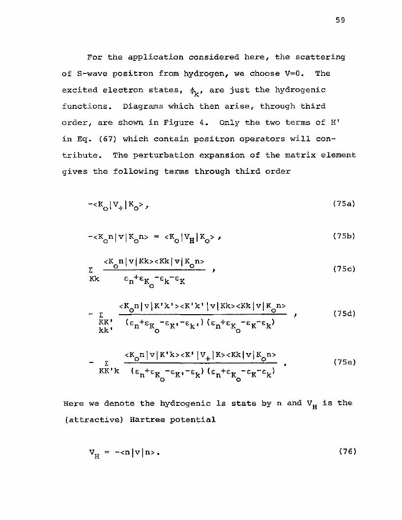
For the application considered here, the scattering of S-wave positron from hydrogen, we choose V=0. The excited electron states, are just the hydrogenicfunctions. Diagrams which then arise, through third order, are shown in Figure 4. Only the two terms of H 1

in Eq. (67) which contain positron operators will con­tribute. The perturbation expansion of the matrix element gives the following terms through third order

(75a)

— <K nlvIK n> = <K IV„|K >, o l i o o 1 H i o (75b)

<K n v KkxKk v K n> o 1 1 1 1 o£ f

Kk en+eK -ek~eKo(75c)

- £<KQn| vjK'k' xK'k' | v| KkxKk |v| KQn>

KK* <En+EK _eK.-ev ,) (en+ev kk' o n K K k' o(75d)

- Z<KQnjvjK'kxK' |V+ |KxKkjv|KQn>

KK k (En+eK ”eK* o(75e)

Here we denote the hydrogenic Is state by n and VH is the (attractive) Hartree potential

Vjj = -<n|v|n>. (76)

60

The standard choice of V, is such as to make the*rfirst-order corrections, Eq. (75a) plus Eq. (75b), vanish. However, the second-order correlation effect, Eq. (75c), is large in this case and we choose V+ in such a manner as to partially compensate for this polarization effect. Pre­liminary calculations including first- and second-order diagrams with intermediate states restricted to the multi­poles &<_3 were performed using four choices of V+: (i)V,=V„ , (ii) V =V„+V(Bethe) where V(Bethe) is the adiabatic+ H + ii

5 5dipole polarization potential, (iii) V+=VH+V(Bethe)+V(Reeh) where V(Reeh) is the adiabatic quadrupole polar-

56ization potential, (iv) V =V„+V(Buckingham) where+ ti

V(Buckingham) = -4.5/(r2 +A2 ) 2 (77)

57and A is used as an adjustable parameter. A value of A-1.85 was found to maximize the second-order results.

Choices (ii), (iii), and (iv) (with A=1.85) were found to give essentially the same second-order phase shifts, with V =V„+V(Bethe) giving slightly larger values.*r ilHowever, choosing V+=Vjj gives decidedly inferior resultsat low energies. This is illustrated in Figure 5 wherewe plot 6 t (Hartree), 6 ^ (Hartree+Bethe), 6 (Hartree),

316 (Hartree+Bethe) and Schwartz's values for 6 . The agree­ment of the second-order phase shifts for all model potentials at the high energy portion of the spectrum

61

infers that the variational method of computing the phase shifts should be quite good away from threshold. The results discussed in the following section were computed using the choice V^V^+VCBethe). However, we shall refert iito the difference between the Schwartz result and the Hartree result as the full correlation correction to the phase shift. The zero energy scattering solution to Eq. ( 6 8b) was found to have no zeros other than at the origin and therefore there exists no bound states of the zero- order positron Hamiltonian, h.

II-4. RESULTS

With the choice V .=V_.+V(Bethe) the first-order con-+ XI

tribution becomes

^ o ^ o p V o - -<K0 |V(Bethe)|K0>, (78)

which is the sum of Eg. (75a) and Eq. (75b). This partially cancels the second-order matrix element Eq.(75e). In Table IX we list the various contributions to 6 through second order. These results are subdivided into the multipole of the intermediate states, and further sub­divided into contributions from bound excited states k(b) and from continuum excited states k(c). Bound f states are not included since their contribution is small. We estimate that an error of about 1 % of the difference between the static results and the exact results is made when one neglects multipoles £>4 in second order. The second-order phase shifts are also plotted in Figure 4.One observes that approximately 67%-80% of the totalcorrelation effect is accounted for in second order. This

3 6is to be compared with the results of Hahn and Spruch who obtain 85%-89% of the full correlation effect using multipoles £<3 and including all orders of interactions.

The radial integrals were performed using Rmax=45.The trial phase shift, 6 t, and the first-order matrix

62

63

element, Eq. (78), were extended to infinity using the

accuracy of the second-order p and d multipole contribu­tions was made by simultaneously computing the adiabatic matrix elements which are obtained by setting equalto £„ in the denominator of Eq. (75c). The results were

ocompared to the matrix elements of the Bethe potential and the Reeh potential and were found to agree to approxi­mately .5%. The latter figure then serves as our esti­mate of the numerical accuracy of the second-order results.

Higher order correlations involving multipoles £.£3are estimated using the third-order diagrams according

51 53to the techniques devised by Kelly. * The most impor­tant intermediate electron states of the second-order matrix element are 2s, 2p, ks~.5s, kpl.Sp, kd~.75d and kfll.Of. Similarly we find that the most important inter­mediate positron states are given by Ks~.75s, Kpl (. 25+.8KQ)p,Kd~(.75+.6 K )d and Kf^(1.25+.6K )f.o o

For a particular I value of the excited states K, k in Fig. 4c, with K, k chosen to be the typical excitations of importance just given, the ratios

<K n|v|K1k'><K'k'|v|Kk>

technique of Levy and Keller. 58 A check on the numerical

t(K,k) = - EK'k'

/<K n 1v|Kk> / o

(79)

64

< K n| v | K ' k x K ' | V . | K >a(K,k) = -2 — --------------±--- /<K n|v|Kk> (80)

K' e +e_,n K K' k o

are constructed. The motivation for forming these ratiosbecomes clear when one compares the third-order matrixelements, Eq. (75d) and Eq. (75e), with the second-ordermatrix element, Eq. (75c). The ratio t has been found by

51 53Kelly ' to be reasonably accurate approximation for the ratio of the ladder diagram, Fig. 4d to the second-order diagram, Fig. 4c. Similarly, a approximates the ratio of Fig. 4e to Fig. 4c.

In order to facilitate the discussion we subdivide the contributions to the ladder approximation, t(K,k), into its diagonal part and its non-diagonal parts. For a given k the diagonal parts considered, tQ (k) are as follows:

k = 2 s ->■ k 1 = 2 s ,k = ks ■+ k * = continuum s /k = 2 p k 1 = 2 p fk = kp -*■ k 1 = continuum p rk = kd -* k' = continuum d, (81)

while the non-diagonal parts considered, tND(k -k')r are

65

k = 2 s ■+ k' = all s ( 2 s),k = ks ■* k' = bound s ,k = 2 p -»■ k* = all s, all p (T p) , all d, all £,k = kp •+ k' = all s, bound p, all d, all £ f

k = kd ■+ k' = bound d. (82)- -j

We have not considered diagonal third-order corrections for intermediate f and bound d states since their contri­bution is small. Similarly, some (presumably small) non­diagonal third-order effects have not been included.

In evaluating Eq. (80) the intermediate matrixelement, <K'| v , |K>, diverges for K'=K if we let R

1 + 1 ' 3 max53approach infinity. However, the integration over K'

removes this infinity. A similar phenomenon occurs for tD(k). Further, there is substantial cancellation between tD (k) and a(k). The third-order ratios have been computed for the energies of interest. In Table X we list the results for the single case Kq=.3.

Higher-order corrections are estimated in the fol­lowing manner. Diagonal ladder diagrams can be summed toall orders since the ratio of the (n+1 )st-order diagram

thto the n -order diagram is approximately given by tD(k)+a(k). The net effect is to modify the second-order diagram associated with the state k by the factor

(l-tD (k)-a(k)) 1 (83)

66

Non-diagonal third-order diagrams contribute a factor

(l~tD (k) -a (k)) _1 ^(k-.k*) {l-tD (k’)“a(k'))-1 . (84)

The transitions considered are given in Eg. (82), A factor of 2 should be included for the a changing third- order non-diagonal diagrams to account for both k-+-k' and k'->-k. We also estimate some small fourth-order diagrams of the type k-*-k'-j-k which give rise to a factor

(l-tD (k)-a (k)) _1 t^D (k-*k') (l-tD (k)-a (k))-1 . (85)

Using these estimates we compute a "coefficient of enhancement", Ce, for each of the second-order contribu­tions listed in Table IX. We have set Ce=l for bound d and continuum f contributions. The Ce value for s and d states includes only the £ non-changing transitions as indicated in Eq. (82). The jl changing corrections have been included in the p state Ce value. These results are listed in Table XI.

The final value of the phase shift is then obtainedfrom

(86)

67

where the summation runs over those contributions to the second-order optical potential listed in Table IX. Table XII contains the results of our calculation and compares them with the variational calculation of Hahn and Spruch?^ The Hahn and Spruch results include multipoles JlO and constitute an accurate estimate of the best results one can obtain with just these multipoles.

The present calculation, which includes only inter­mediate s, p, d and f states contains about 8% less of the full correlation effect than the corresponding calculation of Hahn and Spruch. Subsidiary calculations were performed in which only s, p, d and only s, p states were-included. The difference with the corresponding calculations of Hahn and Spruch were 4% and 1% respectively. The good agree­ment of the results when only s, p states are includedsuggests that the variational approximation used here,Eq. (73), is sufficient if the single-particle potential is properly chosen. We believe the growing discrepancywith increasing multipoles is partly due to the techniques used for estimating the higher-order effects and partly due to the total neglect of fourth-order diagrams of the type s-*-p-*“d, p-*d*+-f, and p*>p'-»-s,d where the first transition i s non-diagonal.

II-5, SUMMARY AND CONCLUSIONS

We have calculated phase shifts for the S-wave scattering of positrons from hydrogen using a many-body optical potential. A single-particle positron potential has been chosen which effectively minimizes third- and higher-order correlations. These higher-order effects are still large and present techniques seriously under­estimate their contribution. In the model problem where only s, pr d intermediate states are allowed to enter, thepresent formulation agrees to within 5% of the ’'exact"

36answer. This is consistent with the results of thetriplet S-wave electron-hydrogen scattering calculation

51of Kelly where only these multipoles are important.The contribution from multipoles £>_3 is known to

36be large. Second-order contributions from these multi­poles have been found to be small in this calculation. Attempts to estimate their contribution in third- andhigher-orders give substantially smaller corrections than

36can be inferred from the calculation of Hahn and Spruch.For this reason we have not attempted to include multi­poles £_>4.

43The optical potential calculation of Drachman in which all multipoles are included in a non-adiabatic manner gives excellent results for the positron-hydrogen problem. However, extension of this formalism to the positron- helium problem necessitated an approximation and the results

68

69

are somewhat poorer. We expected that an application of the present many-body formalism to the positron-helium problem would give better results than those obtained here for the positron-hydrogen case, because the substantially smaller polarizability of helium should give smaller higher-order correlations and smaller errors in estimating them. However, after making a few calculations to the second-order for the positron-helium case, we found that the improvement over the positron-hydrogen case was negli­gible, and the work on the positron-helium problem was discontinued.

TABLE IX: CONTRIBUTIONS TO THE SECOND-ORDER S-WAVE PHASESHIFT (IN RADIANS) FOR POSITRON-HYDROGEN SCATTERING USING THE SINGLE-PARTICLE POSITRON POTENTIAL v+=vHartree+vBethe• THE A VALUE IS THE MULTIPOLE OF THE BOUND (b) OR CONTINUUM (c) EXCITED ELECTRON STATES.

K o 0.0a) 0.1 0.2 0.36 t -1.4587 .0982 .1139 . 0870

v u>op 2.7803 -.2094 -.2836 -.2964

v (2)op (ka, =c0) - .0544 . 0048 .0080 .0104

v <2)op (k£=b0) - .0950 .0083 .0139 .0179

v (2)op (k£=cl) - .6956 . 0545 . 0785 .0871

v (2)op (kS, =bl) -1.4705 .1038 . 1283 .1230

v (2)op (k£=c2) - .1877 .0158 . 0233 . 0255

v (2)op (kJL=b2) - .0250 .0020 .0025 .0022

v (2)op (k&=c3) - .0494 .0042 .0062 .0068

s (2) -1.2561 .0822 .0910 . 0635

a) The K =0 entries are contributions to the scattering length.

70

71

TABLE IX: (CONTINUED)

KO 0.4 0.5 0.6 0.7

6t .0415 -.0102 -.0622 -.1115

<H ft 0

> -.2868 -.2697 -.2509 -.2327

v (2>op (k£=cO) . 0125 .0147 .0171 .0198

v (2)op (k£=bO) .0214 . 0250 . 0291 . 0345

V (2) op (k£=cl) .0890 . 0883 .0860 . 0826

v (2)op (k£=bl) .1106 .0953 .0814 . 0705

v (2) op (k&=c2) .0251 .0235 . 0214 .0191

v (2)op (k£=b2) .0018 . 0013 .0010 . 0007

v <2)op (k£=c3) . 0066 .0060 .0053 .0046

(2)6 .0218 -.0258 -.0719 -.1123

TABLE X: THIRD-ORDER RATIOS FOR K =.3o

tQ(2s)+a(2s) -.5487

tD (ks)+a(ks) -.2808

tD(2p)+a(2p) -.0478

tD (kp)+a(kp) -.0017

tD (kd)+a(kd) . 0627

tBD(2s'*S) ,1188

^ ^ 8 - 6 ) .1461

W 2***1 -.0398

t^up-p) . 0818

.0660

tND(2p-vf) .0184

t^lkp-s) .0053

tND(kp*p) .0742

tND(kp"a> .0343

tj,D (kp-f) .0054

tND(ka-a) .0139

72

TABLE XI: Ce VALUES

Ce(bO) Ce(cO) Ce(bl) Ce(cl) Ce(c2)

.7262 .8735 1.1260 .9956 1.0646

7265 .8733 1.1521 1.0646 1.0754

7216 .8713 1.1649 1.1181 1.0811

7115 .8675 1.1644 1.1561 1.0817

6968 .8620 1.1475 1.1755 1.0755

.6758 .8544 1.1237 1.1859 1.0679

.6425 .8442 1.1031 1.1963 1.0627

.5989 .8316 1.0822 1.2036 1.0585

TABLE

K o

XII: POSITRON-HYDROGEN

Hartree ThisCalculation*5

PHASE SHIFTS IN

Hahn and Spruch*5}

RADIANS

Schwartz

o .oa) .5822 -1.4091 OH•c\]1

.1 -.0580 . 0996 .151

.2 -.1145 .1187 .142 .188

.3 -.1682 .0938 .168

.4 -.2181 . 0488 .076 .120

.5 -.2635 - .0043 .062

.6 -.3042 - .0540 -.029 .007

.7 -.3400 - .1038 -.054

a) The Ko=0 entries are scattering lengths

b) Including multipoles JL<3

74

FIGURE CAPTIONS

Figure 1

Figure 2

Figure 3

Figure 4

Figure 5

Poles and branch cuts in the single channel and coupled channel S-matrix.Hartree-Fock energy levels for Li and the multiconfiguration Hartree-Fock ground state and metastable excited states of Li . Hartree-Fock energy levels for Na and the multiconfiguration Hartree-Fock ground state and metastable excited states of Na . Contributing diagrams to <K0 lv0plK0> through third order.S-wave positron-hydrogen phase shifts inradians. 6 =Schwartz results, 6.=zero-order

(21results, 6 =second-order results. H=Hartreesingle-particle potential, H+B=Hartree plus Bethe single-particle potential.

75

76

E plane

(a) °— o-Ej E2 E3

(b)B

E plane

E.

oRi

E plane

(c)

(d) B

E2r2

R 3E plane

E, E; a—o R 2

Ri or 3

Fig. 1

' / L i * lsz (' S ) 0 .3 9 2 6 %

Li lsg3d (gD) 0.2815 Li ls23p (g P) 0.2796

Li ls23s (gS) 0.2457

Li" (>P) 0.2776. Li” <3P) 0.2761 Li" CS) 0.2727\ Li" CD) 0.2718v Li" (3S) 0.2456\ Li“ (3P) 0.2398\ Li“ CS) 0 .22 8 6

Li ls22 p (2P) 0.1353

Li ls22s(2S) 0 .0

L i ' fS ) -0.0451

78

/* / .' /N o * Is22s22p6 CS) 0.3636z

No Is2 2sa2p64p(2P) 0.2632 No ls22s22p63d (2D) 0.2523

No ls22s22 p6 4s (2S)0.2235No ( i

No ls22s22p63p (2P) 0.1453

No lsg2sz2p63s(2S) 0.0

No* CS

) 0.2125

) -0.0394

Fig. 3

79

A , f OI 1 1 JCI I I v— I..*"- |

)

llll! 2 ■■J*<£-

*v . i ;O o 1 ■xl ^ S i

^---N ----VCQ XL XL XL

1 5---i---*-=- C

■ VO

XL

*• * iC ^j 1 JC J

I i i * ! i ! i !! o B ! ,-a3 -l,J,v ------ N ----a*'ro 0 - 0 —^ -----0----- ^ ^ V V V

o o XL XL

Fig. 4

80

0.2

0.1

S (2)(h+b )0.08 <2>(H)

- 0.1

- 0.2

- 0.3

- 0.40.2 0.3 0.4 0.5 06 0.70 0.1

K 0 ( a 2 )

Fig. 5

REFERENCES

1. B. L. Moiseiwitsch, Advances in Atomic and Molecular Physics, Vol. I, edited by D. R. Bates and I. Ester- mann (Academic Press, Inc., New York, 1965), p. 61.

2. G. Glockler, Phys. Rev. 46, 111 (1934).3. B. Edlen, J. Chem. Phys. J3, 98 (1960).4. M. Kaufman, Astrophysics J. 137, 1296 (1963).5. R. J. S. Crossley, Proc. Phys. Soc. (London) 83 375

(1964).6. H. R. Johnson and F. Rohrlich, J. Chem. PHys. 30,

1608 (1959).7. A. W. Weiss, Phys. Rev. 122, 1826 (1961).8. E. Clementi and A. D. McLean, Phys, Rev. 133, 419

(1964).9. A. W. Weiss, Phys. Rev. 166, 70 (1968).10. B. Ya'akobi, Phys. Letters 2j3, 655 (1966).11. Atomic Energy Levels, edited by C. E. Moore, National

Bureau of Standards Circular No. 467 (U.S. Government Printing Office, Washington, D. C. 1949) .

12. A. Salmons and M. J. Seaton, Proc. Phys. Soc. (London)77, 617 (1961).

13. E. Clementi, Tables of Atomic Functions, (IBM Corp., San Jose, 1965).

214. We use the set of units J4=2m=e /2=1.

15. E. U. Condon and G. H. Shortley, The Theory of Atomic

81

82

Spectra, (Cambridge, 1953).16. I. C. Percival and M. J. Seaton, Proc. Camb. Phil.

Soc. S3, 654 (1957).17. J. J. Matese and R. S. Oberoi, Phys. Rev. (to be

published).18. H. P. Kelly, Phys. Rev. 131, 684 (1963).19. C. L. Pekeris, Phys. Rev. 112, 1649 (1958); 115, 1216

(1959).20. C. C. J. Roothaan, L. M. Sachs and A. W. Weiss, Rev.

Mod. Phys. 3£, 186 (1960).21. E. M. Karule and R. K. Peterkop, Opt. i Spektroskopiya

16, 958 (1964) (Eng. Transl.: Opt. Spectry. (USSR)16, 519 (1964)); G. E. Chamberlain and J. C. Zorn, Phys. Rev. 129, 677 (1963).

22. H. P. Kelly, Phys. Rev. 136, 896 (1964).23. H. Feshbach, Ann. Phys. (N.Y.) 5_, 357 (1958); 19,

287 (1962).24. Y. Hahn, T. F. O'Malley and L. Spruch, Phys. Rev. 128,

932 (1962).25. T. F. O'Malley and S. Geltman, Phys. Rev. 137, A1344

(1965).26. L. Lipsky and A. Russek, Phys, Rev. 142, 59 (1966).27. P. G. Burke, Advances in Atomic and Molecular Physics,

Vol. IV, edited by D. R. Bates and I. Estermann (Academic Press, Inc., New York, 1968), p. 189.

83

28. E. M. Karule and R. K. Peterkop, JILA Information Center Report No. 3, University of Colorado, Boulder, Colorado (1966) (unpublished).

29. P. G. Burke and A. J. Taylor, Theoretical Physics Division, A.E.R.E., Harwell, Didcot, Berks. (1969) (unpublished).

30. J. Perel, P. Englander and B. Bederson, Phys. Rev.128, 1148 (1962).

31. C. Schwartz, Phys. Rev. 124, 1468 (1961).32. R. J. Drachman, Phys. Rev. 138, A1582 (1965).33. J. Callaway, R. W. LaBahn, R. T. Pu, and W. M. Duxler,

Phys. Rev. 168, 12 (1968).34. Y. Hahn, T. F. O'Malley, and L. Spruch, Phys. Rev.

130, 381 (1963).35. P. G. Burke and A. J. Taylor, Proc. Phys. Soc.

(London) 88, 549 (1966).36. Y. Hahn and L. Spruch, Phys. Rev. 140, A18 (1965).37. P. G. Burke and H. M. Schey, Phys. Rev. 126, 147

(1962).38. P. G. Burke and K. Smith, Rev. Mod, Phys. 21/ 458

(1962).39. R. J. Damburg and E. Karule, Proc. Phys. Soc. (London)

90., 637 (1967) .40. R. J. Damburg and S. Geltman, Phys. Rev. Letters 20,

485 (1968).41. J. F. Perkins, Phys. Rev. 173, 164 (1968).

84

42. P. G. Burke, D. P. GalXaher and S. Geltman, J. Phys.B. 2, 1142 (1969) .

43. R. J. Drachman, Phys. Rev. 173, 190 (1968).44. M. Gailitis, Zh. Eksperim i Teo. Fiz. 47^ 160 (1964)

(English transl.: Soviet Phys. ~JETP 2j0, 107 (1965)).45. R. S. Oberoi and J. Callaway, Phys. Letters 3QA, 419

(1969).46. M. H. Mittleman and K. M. Watson, Phys. Rev. 113, 198

(1959).47. J. S. Bell and E. J. Squires, Phys. Rev. Letters 3

961 (1959).48. K. A. Brueckner, The Many-Body Problem (John Wiley &

Sons, Inc., New York, 1959).49. J. Goldstone, Proc. Roy, Soc. (London) A239, 267

(1957) .50. R. T. Pu and E. S. Chang, Phys. Rev. 151, 31 (1966).51. H. P. Kelly, Phys, Rev. 160, 44 (1967).52. Upper case letters denote positron quantities and

lower case letters denote electron quantities.53. H. P. Kelly, Phys. Rev. 144, 39 (1966); 152, 62 (1966).54. T. Y. Wu and T. Ohmura, Quantum Theory of Scattering

(Prentice-Hall, Inc., Englewood Cliffs, New Jersey, 1962), p. 59.

55. H. A. Bethe, Handbuch der Physik (Edwards Brothers, Inc., Ann Arbor, Michigan, 1943), Vol. 24, Part 1, pp. 339 ff.

85

56. H. Reeh, Z. Naturforsch. 150, 377 (1960).57. R. A. Buckingham, Proc. Roy. Soc. (London) A16 0,

94 (1937).58. B. R. Levy and J. B. Keller, J. Math. Phys. 4_, 54

(1963).

APPENDIX I

This appendix demonstrates the method used to evalu­ate integrals which involve products of two determinantal wave functions.

Let

A = DN (a1a2...aN)7 (AI-1)

and

B = DN Cb1b2...bN), CAI-2)

where D's are determinants of the form of Eq, (9) of the main text, and a , b belong to an orthonormal set of functions. In order that A and B are not identically zero, we must have

<ai|aj> = 6 ij, (AI-3)

and

<b. lb.> = 6. . . (AI-4)r 1 3 1 3 •

Let us also assume that A and B are permuted so that most elements are identical in pairs, a^=b^,••«a^=b^,•••,

86

87

except, maybe, and at^bt-We wish to evaluate

<A|P j B> (AI-5)

in which F are one- or two-particle operators. Let us expand A and B in a manner so that similar terms appear at corresponding locations in the expansion,

a = ------ { a , a „ » » * a _ ± • • » + a , a, # • 'a, • • • a , • • * i a . 3. •1“lei2 T5 i j k t i i/ N ! J J

1B = --- {b.,b_••-b„±•••±b.b.***b1 •**b, •••±b.b .,/gr 1 2 N 1 3 k t x ]

b _ * • • b^ ,

(1) F = 1.

It is easy to see that <A|B>=0 unless A=B, since the general term of (AI-5) is

ca.lb.xa. |a„>***<a lb > (AI-6)N ! 3L* D k 1 H, y' z

and is 0 unless the two elements in each pair are equal, or A=B. (We do not consider the case A=-B, since it is

88

trivial.)For each term in A, the only non-vanishing product

comes from a term in B which occupies the corresponding location as the term in A. There are a total of N! terms in the product, therefore,

<A|A> = 1 . (AI-7)

N(2) F = s f(i)/ and B differs from A only in a.^b, .

i

The non-vanishing terms in the product must containXthe factor <at |f|bt>, and each xs equal to <at|f|bt>.

Again, each term in A contributes one such term in the product, therefore.

<A|F|B> = <at |f|bt> . (AI-8)

If A=B, then we may treat each a^ as a ., thus

N<A|F|A> = S <a^|f)ai> , (AI-9)

N(3) F = Z g(i#j)r and B differs from A only in a^b , a ^ b f

In this case, for each term in A, not only the corre­sponding term in B contributes, but also the term with k

89

and t exchanged, except that the latter product takes a (-) sign. Therefore,

<a |f |b > = <akatJgibkbt>-<akat lglbtbk> • (Al-10)

If ak=bk/ but at^b / we may treat each a^, except at, as ak,

N<a |F1B> = ^ [<aiat lglaibt>-<aiat |glbtai>] . (AI-11)

If A=B,

N N<a |f |a > = E £ [<a.a.IgI a.a .>-<a.a.|gI a .a.>], (AI-12)i>j i j 13 1 n i

These results were obtained by Condon and Shortley, but the above presentation is quite different from theirs. To apply this method to our problem, we consider the following cases.

{4) F = 1, and B differs from A only in aN^bN and they satisfy the conditions

<aN lbi> = <bNIai> = 0 ' i=l,2,-*-N-l ,

but

<aN l bN> *

90

The general term of <A1B>, similar to Eq. (AI-6), is 0 unless a^ pairs with b^, i=l,2,*»»N, and its value is —y- <aN |bN>. There are N! terms, therefore,

<A]B> = <aN |bN> . (AI-13)

(5) F = 1, and B differs from A in aN_^bN_1, ' an<they satisfy the conditions

but

<a.]b.> = <a.|b.> = 0 , j=N-l,N; i=l,2,***N-2 ; 3 1 j* 3

There are two groups of non-vanishing terms in <a |b >now. One group contains terms similar to those of (4),that is, a^ pairs with b^, i=l,2,••*N, and each term is *1NT <aN-l!bN-l><aNlbN>' The other ?rouP contains terms similar to the above but with b^ and bN_- exchanged. Since there is one more exchange in one determinant than in the other, we need a (-) sign. Each term in the second group is - iy <aN_ilfaN><aN lbN_1>- Each group has N! terms, therefore,

<A|B> <aNlbN><aN-ll£,N-l>“<aNlI:)N-l><aN-l^bN>*

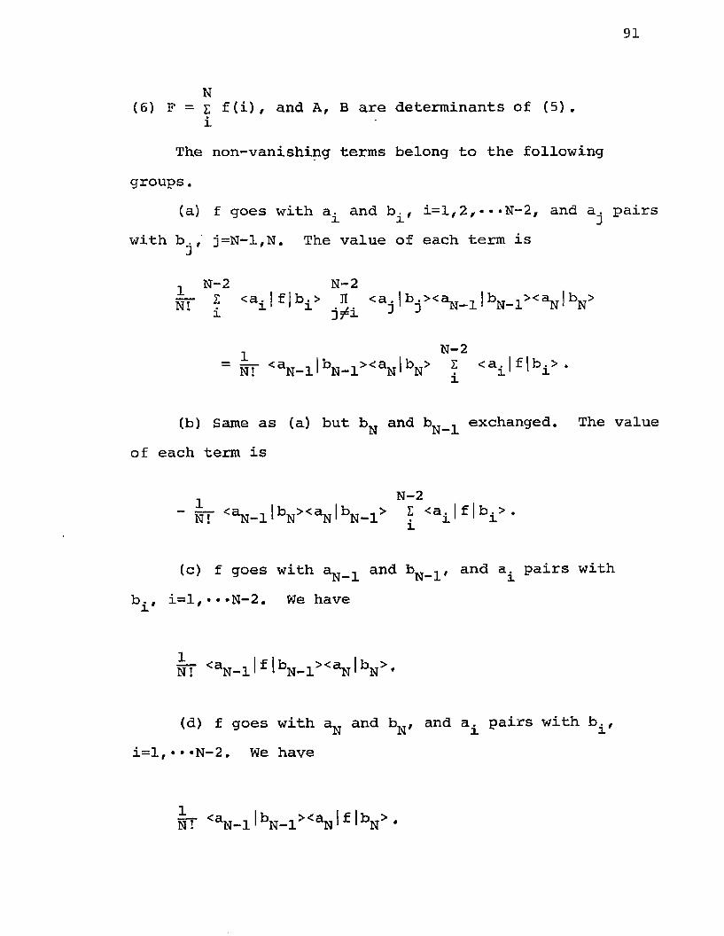
91

N(6) F = £ f(i), and A, B are determinants of (5).

iThe non-vanishing terms belong to the following

groups.(a) f goes with a^ and b^, i=l,2,••*N-2, and a pairs

with b^, j=N-l,N. The value of each term is

N-2 N-2‘j1 j > 1 ' N-l w 1 N

, N-2= NT <aN - l l bN - l ><aN l V I < a l l f I V -

(b) Same as (a) but bN and t>N_1 exchanged. The value of each term is

N-2N! <aN-llbN><aNlbN-l> ? <aiIfIbi> *

(c) f goes with a ^ ^ and and aj_ pairs withb., i=l,»*»N-2. We have r' '

N! <aN—llflbN—l><aNlbN>*

(d) f goes with aN and b^, and a^ pairs with b , i=lr***N-2. We have

N! <aN-llbN“l><aN^f lbN> *

92

<e) Similar terms as in (c) and (d) but withand bN_^ exchanged. Again we need a (-*) sign, therefore,

NT *<aN-llf bN><aNlbN-l> + <aN-l^bN><aN^f

The number of terms in each group is N !, therefore,<a |f |b > is the sum of the above multiplied by N !. Theresult is given in Eg. (15) of the main text.

N(7) F = E g(ifj)r and A, B are determinants of (5).

i> jThe non-vanishing terms belong to the following

groups.

(a) g goes with a^, a and b^, b^, i,j=l,* ■ *N-2, anda^ pairs with b^,k=N-l,N. Each term is

1 N-2BT Z <aiaj|9|bibj><aN-llbN-l><an l V *X ]

(b) Same as (a) but b^ and b^ exchanged. The term value is

1 N~2NT <aiajlg lbjbi><aN-llbN-l><aNlbN> *

(c) g goes with a^, a^_^ and b_ , i=l,***N-2, and a pairs with b , j=l,..-N, but jj i and j^N-1. The term value is

93

1 N-2iff I <aiaN-ll9lbib8-l><aHl1V -

(d) Same as (c) but and b^^ exchanged. The termis

x N-2" in | <aiaN-il9lbN-ibi><aN l V -

(e) Same as (c) and (d) but exchange aN-1r bN-i witJla^, bN» Since there are two more exchanges, the (-) signis not needed. The sum of the two terms is

± N-2ST I {<aiaNl9lbi V <aH-llbN-l>

<aiaN 1 lbNbi><aN-lIbN-l> •

(f) g goes with aN_1# and b^, and a^ pairswith b^, i=l,*»»N-2. The term value is

FIT <aN-laNlg lbN-lbN> *

(g) All of the above groups from (a) to (f) but with fc>N-l and bN exchanged. We, of course, need an extra (-) sign again.

The sum of all terms in the groups, (a) to (g), multi­plied by N! gives the result of Eq. (16) of the main text.

VITA

Albert Ai-Chun Fung, son of Yu-Chin and Shih (Chang) Fung, was born in Tunghsien, Hopei, China, on September 16, 1917. He attended Yu-Ying Primary School and Peiping Practiced Middle School. He graduated in June 1935, and entered Peiping Normal University as a physics major.When the Sino-Japanese War broke in 19 37, he transferred to Chiaotung University, Kweichow, China, and changed his major to Mining and Metallurgical Engineering. He re­ceived his Bachelor of Engineering degree in June 1941.He married Fefe, daughter of Jen-Jung and Wang Huang, on May 27, 1943. They have three daughters and a son. He was a Petroleum Engineer with Chinese Petroleum Corpora­tion until January 1957, when he entered the Graduate School of Saint Louis University in physics, and received his Master of Science degree in January 1959, and became a member of The Society of The Sigma xi in the same year. He was an Instructor in Physics at Whittier College, Whittier, California, from 1959 to 1967. In September 1967, he entered Louisiana State University on a teaching assistantship and is presently a candidate for the degree of Doctor of Philosophy in the Department of Physics and Astronomy.

94

EXAMINATION AND THESIS REPORT

Candidate: Albert Al-Chun Fung

Major Field: Physics

Title of Thesis: Atomic Systems with a Closed Core Plus Two Electrons

Approved:

ajor Professor and Chairman

Dean of ihe Graduate School

E X A M IN IN G COM M ITTEE:

_______ ' F 1 U<. C __________

Date of Exam ination:

July 15, 1971