Atlantic Forest - Appendix

Collection 4

Version 1

General coordinator

Marcos Reis Rosa

Team

Fernando Frizeira Paternost

Jacqueline Freitas

Viviane Cristina Mazin

Eduardo Reis Rosa

1. Overview of classification method

The production of the Collection 4, with land cover and land use annual maps for the

period of 1985-2018, followed a sequence of steps in the Atlantic Forest biome, similar to

those used in the previous Collection 3.1 (Figure 1). However, some improvements were

added up, particularly in the geographical units for classification, balance of samples and in

the post classification filters.

Figure 1. Classification process of Collection 4 in the Atlantic Forest biome.

2. Landsat image mosaics

2.1. Definition of the temporal period

The image selection period for the Atlantic Forest biome was defined aiming to maximize the coverage of Landsat images after cloud removing/masking.

Despite the diversity of ecosystems and the great extent of the biome (Figure 2), both in latitudinal amplitude and in coast extension, the Atlantic Forest has a well-defined dry period between the months of April to September (Figure 3).

Figure 2. Native vegetation types in the Atlantic Forest biome (IBGE, 2017).

Figure 3. Monthly precipitation values of the period from November 20, 1997 to November 20, 1998, in Cunha-SP (ARCOVA et al., 2003).

2.2. Image selection

For the selection of Landsat scenes to build the mosaics of each chart for each year, within the acceptable period, a threshold of 50% of cloud cover was applied (i.e., any available scene with up to 50% of cloud cover was accepted). This limit was established based on a visual analysis, after many trials observing the results of the could removing/masking algorithm. When needed, due to excessive cloud cover and/or lack of data, the acceptable period was extended to encompass a larger number of scenes in order to allow the generation of a mosaic without holes. Whenever possible, this was made by including months in the beginning of the period, in the winter season.

In most cases the period from April 1st to August 30th was good to get a mosaic with none or few missing information caused by clouds and shades. In some specific cases it was needed to extend significantly the temporal period to include images from September and October.

In the Northeast states the period was February 1st to 30 of October to maximize the visible areas and avoid missing areas caused by clouds.

For each year we used images from the best Landsat available:

● 1985 to 1999 – Landsat 5

● 2000 to 2002 – Landsat 7

● 2003 to 2011 – Landsat 5

● 2012 – Landsat 7

● 2013 to 2017 – Landsat 8

2.3. Final quality

As a result of the selection criteria, most of mosaics presented satisfactory quality. Northeast of Brazil and some regions in Santa Catarina and São Paulo offer more challenge to build clean mosaics and the information still has some noise or missing data.

3. Definition of regions for classification The classification was done in homogenous regions to reduce confusion of samples and classes, as well as to allow a better balance of samples and results. The Atlantic Forest biome was divided in 30 regions based in (Figure 4):

Figure 4. Regions used in the classification of Atlantic Forest biome.

4. Classification

4.1. Classification scheme

The digital classification of the Landsat mosaics for the Atlantic Forest biome aimed to individualize a subset of eight land cover and land use classes from the complete legend of MapBiomas Collection 4 (Table 1), which were integrated with the cross-cutting themes in a further step.

Table 1. Land cover and land use categories considered for digital classification of Landsat mosaics for the Atlantic Forest biome in the MapBiomas Collection 4.

Legend class of Collection 4 Numeric ID C

Color

1.1.1. Forest Formation 3

1.1.2. Savanna Formation 4

2.2. Grassland Formation 12

2.2. Wetlands Formation 13

3.3 Mosaic of Agriculture or Pasture 21

4.4. Rocky Outcrop 29

4.5. Other non vegetated area 25

5. Water 26

6. Non Observed 27

Exceptionally, in regions 01, 10, 19, 21, 27 and 30 we also included the class 3.2.1

Annual and Perennial Crop (id: 19) and in regions 01, 03, 08, 10, 13, 15, 23, 24, 28 and 30 we

also included the class 1.2 Forest Plantations (id: 9).

4.2 Feature space

The feature space for digital classification of the categories of interest for the Atlantic Forest biome comprised a subset of 31 variables (Table 2), taken from the complete feature space of MapBiomas Collection 4. They include the original Landsat reflectance bands, as well as vegetation indexes, spectral mixture modeling-derived variables, terrain morphometry (slope), and a spatial texture measure. The definition of the subset was made based on the expected usefulness of each variable to discriminate the targets of concern, considering local knowledge about their spectral, spatial and temporal dynamics.

Table 2. Feature space subset considered in the classification of the Atlantic Forest biome Landsat image mosaics in the MapBiomas Collection 4 (1985-2018).

'median_gcvi_wet',

'median_gcvi',

'median_gcvi_dry',

'slope',

'textG',

"median_blue",

"median_evi2",

"median_green",

"median_red",

"median_nir",

"median_swir1",

"median_swir2",

"median_gv",

"median_gvs",

"median_npv",

"median_soil",

"median_shade",

"median_ndfi",

"median_ndfi_wet",

"median_ndvi",

"median_ndvi_dry",

"median_ndvi_wet",

"median_ndwi",

"median_ndwi_wet",

"median_savi",

"median_sefi",

"stdDev_ndfi",

"stdDev_sefi",

"stdDev_soil",

"stdDev_npv",

"amp_ndwi"

4.3. Classification algorithm, training samples and parameters

Digital classification was performed region by region, year by year, using a Random Forest algorithm (Breiman, 2001) available in Google Earth Engine, running 60 iterations (random forest trees). Training samples for each region were defined following a strategy of using pixels for which the land cover and land use remained the same along the 33 years of Collection 3.1, so named “stable samples”. An ensemble taken from three main sources was made: extracted from Collection 3.1; manually drawn polygons; and complementary samples.

4.3.1. Stable samples from collection 3.1 The extraction of stable samples from the previous Collection 3.1 followed several

steps aiming to ensure their confidence for use as training areas.First, based on a visual analysis, a threshold was established for each class, specifying a minimum number of years in which a pixel should remained with that class to be eligible as a stable sample. A layer of pixels with a stable classification along the 33 years of Collection 3.1 was then generated by applying such thresholds. From the resulting layer of stable samples, a subset 7,000 samples were randomly generated and balanced for each class based on the class cover percentage. A Minimum of 700 samples used to rare classe that does not cover at least 10% of the region area.

4.3.2. Complementary samples

The need for complementary samples was evaluated by visual inspection and by comparing the output of the preliminary classification with 5.000 validation points used in collection 3.1. Complementary sample collection was also done drawing polygons using Google Earth Engine Code Editor. The same concept of stable samples was applied, checking the false-color composites of the Landsat mosaics for all the 34 years during the polygon drawing. Based in the knowledge of each region, polygon samples from each class were collected and the number of random points in these polygons were defined to balance the samples.

4.3.3. Final classification Final classification was performed for all regions and years with stable and

complementary samples. All years used the same subset of samples and it was trained in the same mosaic of the year that was classified.

5. Post-classification

Due to the pixel-based classification method and the long temporal series, a list of

post-classification spatial and temporal filters was applied. The post-classification process includes the application of gap-fill, temporal, spatial and frequency filters.The temporal filter rules were adapted for the land cover and land use classes used in the Atlantic Forest biome and were complemented by specific rules to adjust for cases where a pixel appeared.

5.1. Gap Fill filter

In this filter, no-data values (“gaps”) are theoretically not allowed and are replaced

by the temporally nearest valid classification. In this procedure, if no “future” valid position

is available, then the no-data value is replaced by its previous valid class. Therefore, gaps

should only exist if a given pixel has been permanently classified as no-data throughout the

entire temporal domain.

5.2. Spatial filter

The spatial filter avoid unwanted modifications to the edges of the pixel groups

(blobs), a spatial filter was built based on the "connectedPixelCount" function. Native to the

GEE platform, this function locates connected components (neighbours) that share the same

pixel value. Thus, only pixels that do not share connections to a predefined number of

identical neighbours are considered isolated. In this filter, at least six connected pixels are

needed to reach the minimum connection value. Consequently, the minimum mapping unit

is directly affected by the spatial filter applied, and it was defined as 6pixels (~0,5 ha).

5.3. Temporal filter

The temporal filter uses the subsequent years to replace pixels that has invalid

transitions.

In the first process the filter looks any native vegetation class (3, 4, 12, 13) that is not

this class in 85 and is equal in 86 and 87 and then corrects 85 value to avoid any

regeneration in the first year.

In the second process the filter looks pixel value in 2018 that is not 21 (Mosaic of

Agriculture and Pasture) and is equal 21 in 2016 and 2017. The value in 2018 is then

converted to 21 to avoid any regeneration in the last year.

The third process looks in a 3-year moving window to correct any value that is

changed in the middle year and return to the same class next year. This process is applied in

this order: [33, 13, 4, 29, 21, 3, 12].

The last process is similar to the third process but it is a 4- and 5-years moving

window that corrects all middle years.

5.4. Frequency filter

Frequency filters were applied only in pixels that were considered “stable native

vegetation” (at least 33 years as [3, 4, 12, 13]). If a “stable native vegetation” pixel is at least

80% of years of the same class, all years are changed to this class. The result of these

frequency filters is a classification with more stable classification between native classes

(e.g. Forest and Savanna). Another important result is the removal of noises in the first and

last year in the classification.

5.5. Incident filter

An incident filter were applied to remove pixels that change too much times in the

34 years. All pixels that changes more than eight times and is connected to less than 6 pixels

that also changes more than eight times is replaced by the MODE value. This avoids changes

in the border of the classes.

All forest pixels that change more than ten times and are connected to less than 66

pixels that also changes more than ten times is replaced to 21 (Mosaic of Pasture and

Agriculture). Forests are stable and these areas that changes this much are not forest.

All forest pixels that changes more than eight times and is connected to more than

66 pixels that also changes more than eight times is replaced to 21 (Mosaic of Pasture and

Agriculture). These areas are also some type of anthropogenic use.

6. Validation strategies

A new set of 14.487 independent validation points provided by Lapig (Laboratório de

Processamento de Imagens e Geoprocessamento - UFG) was used to perform accuracy analysis (Figure 5).

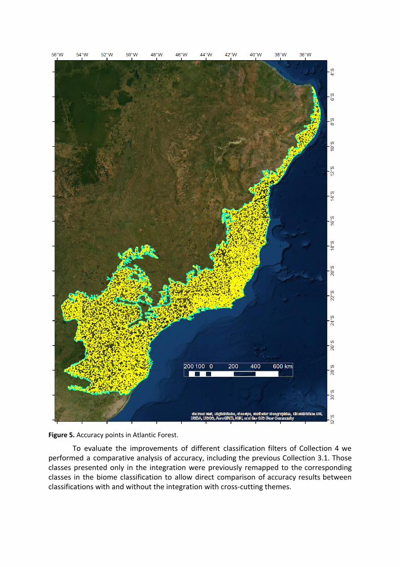
Figure 5. Accuracy points in Atlantic Forest.

To evaluate the improvements of different classification filters of Collection 4 we performed a comparative analysis of accuracy, including the previous Collection 3.1. Those classes presented only in the integration were previously remapped to the corresponding classes in the biome classification to allow direct comparison of accuracy results between classifications with and without the integration with cross-cutting themes.

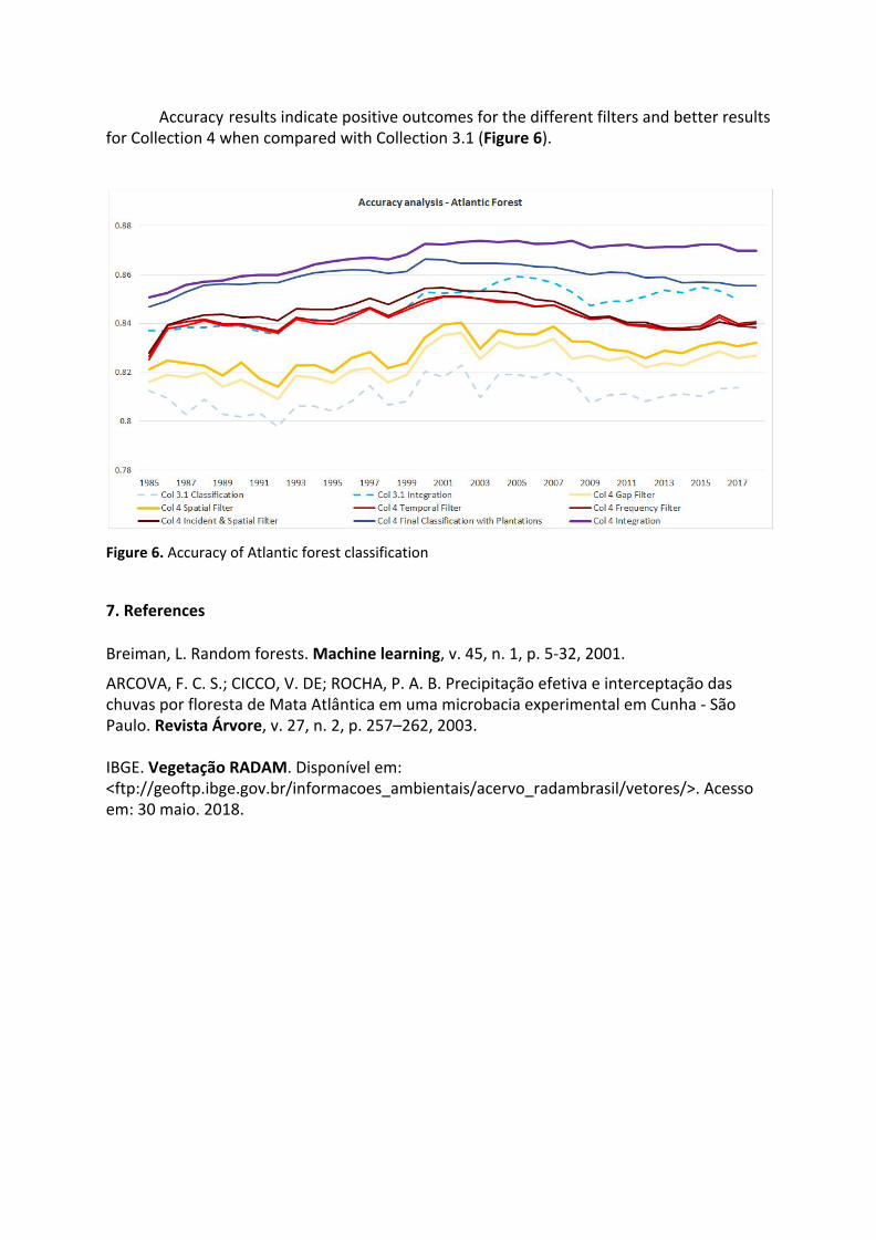
Accuracy results indicate positive outcomes for the different filters and better results for Collection 4 when compared with Collection 3.1 (Figure 6).

Figure 6. Accuracy of Atlantic forest classification

7. References Breiman, L. Random forests. Machine learning, v. 45, n. 1, p. 5-32, 2001.

ARCOVA, F. C. S.; CICCO, V. DE; ROCHA, P. A. B. Precipitação efetiva e interceptação das chuvas por floresta de Mata Atlântica em uma microbacia experimental em Cunha - São Paulo. Revista Árvore, v. 27, n. 2, p. 257–262, 2003. IBGE. Vegetação RADAM. Disponível em: <ftp://geoftp.ibge.gov.br/informacoes_ambientais/acervo_radambrasil/vetores/>. Acesso em: 30 maio. 2018.