JOURNAL OF MATHEMATICAL ANALYSIS AND APPLICATIONS 168, 147-162 (1992)

Asymptotic Theory for a Class of Nonautonomous Delay Differential Equations

J. R. HADDOCK

Department of Mathematical Sciences, Memphis State University, Memphis, Tennessee 38152

AND

Y. KUANC

Department of Mathematics, Arizona State University, Tempe, Arizona 85287-1804

Submitted by V. Lakshmikantham

Received June 18, 1990

This paper deals with asymptotic behavior of solutions of the nonlinear nonautonomous delay differential equation

x’(t) = - I’ .f(t> x(s)) 44t, 31, l-r,,) (*)

where xf( t, X) > 0, f( t, 0) = 0, t - r(f) nondecreasing, p( I, S) is nondecreasing and of bounded variation. General sufficient conditions, which are easy to verify, are obtained for the solutions to be bounded and asymptotically stable (locally and globally). These results improve many existing ones principally by allowing: (i) r(t) to be unbounded, (ii) both discrete and distributed delays, and (iii) the equation to be strongly nonlinear and nonautonomous. Various examples are given in the form of corollaries with a highly flexible integrand. 0 1992 Academic Press, Inc.

1. INTRODUCTION

In 1965, R. Bellman [3] raised the question of the behavior of solutions of the functional differential equation

u’(t)+au(t-r(t))=0 (1.1)

when the delay function r(r) is nearly constant for large t, and also asked for conditions on the function r(l), under which all solutions tend to zero

147 0022-247X/92 $5.00

Copynght c’ 1992 by Academic Press, Inc. All rights of repraductmn I” any form reserved.

148 HADDOCK AND KUANG

as t -+ +co. In response to these questions, K. L. Cooke [bS] investigated the following state dependent delay equation

u’(t)+au(t-r(u(t)))=O, a>0 (1.2)

as well as general linear equations. Under the conditions that either the delay is asymptotically zero (see [bS] for precise statements), and/or its mean value for t b 0 is zero, Cooke obtained various sharp results regarding the asymptotical behavior of solutions of (1.1) and (1.2).

Partly motivated by Cooke’s work, many authors have since contributed to the study of asymptotic behavior of scalar differential equations. (See [l-2, 4, 5, 12-14, 16-221 and the references cited therein.) In particular, the sharp and fundamental work of Yorke [22] influenced several recent papers along this direction. A main assumption of Yorke’s work is that the delay be bounded and the right-hand side of the equation satisfies the so-called Yorke condition (cf. [22, 201 for the precise definition). A modified version of Razumikhin’s theorem (see [8, 221) was applied.

In this paper, we study the following general nonlinear nonautonomous delay differential equation

which includes

x’(t)= - i q(t)f(t,x(t-rri(t))) i=l

(1.4)

and

x’(t)= -[’ f(t, x(s)) 4~ s) ds f--r(t)

(1.5)

as special cases. Here we assume r(t), r,(t), a,(t), f(t, x), k(t, s) are continuous with respect to their arguments. ~(t, s) is of bounded variation. In particular, r(t) may be unbounded, and f( t, x) is any function satisfying xf(t, x) 2 0, f(t, 0) = 0. Thus x(t) E 0 is a solution of (1.3).

We are able to establish sufficient conditions for the solutions of (1.3) to be bounded and for locally or globally asymptotically stable of the zero solution. In all these cases, we give estimates on the supreme bound of solutions and the size of the region -of attraction. These conditions are general, easy to verify, and improve several of the existing ones. In order to illustrate their applications, various examples are given (in the form of corollaries).

ASYMPTOTIC THEORY 149

Our approach, to some extent, is related to the essence of Razumikhin’s theorem. Under proper assumptions, we can easily prove that solutions either tend to zero, or are oscillatory. In the latter case, roughly speaking, we can show, under some conditions, that the local maximum of x(t) over a certain length interval is decreasing.

In the next section, we describe our equation in detail, and present a simple, but important, lemma. Section 3 deals with linear equations and we give the particular equation

x’(t)= -a(t)x(t)-b(t)x(t-r(t)), (1.6)

a special treatment. Nonlinear equations are studied in the last section, where various situations are discussed. Comparisons with existing results are presented throughout.

2. PRELIMINARIES

In this paper, we consider the following general first order real scalar delay differential equation

x’(t) = - 1’ f(c x(s)) 446 s), r-r(r) (2-l 1

where f(t, X) and r(t) are continuous with respect to their arguments, ~(t, s) is continuous with respect to t, nondecreasing with respect to s, and is defined for all (t, s) E R2. In addition, we always assume:

(Hl) xf(t,x)>O, andf(t,x)=O if and only if x=0, (H2) r(t)>O, t-r(t) is nondecreasing, and lim,, .+,(t-r(t))=

+a, W3) 146 t) > At, t - r(t)).

Let r = r(O), then initial value problem for (2.1) takes the form

XC@ = 4(0 BE C-r,Ol, (2.2)

where #(0) E C = C( [ -r, 01, R), where C denotes the space of continuous functions that map the interval C-r, 0] into R. For 4 E C, the norm of 4 is defined by 11411 =max-.G,G, /d(e)/. By [15, Theorem 2.2.11, we know there is at least one solution for the initial value problem (2.1)-(2.2).

Clearly, assumption (i) implies that x(t) - 0, t > 0, is a solution of (2.1) with zero initial function. We say a function x(t) defined on C-r, cc) is oscillatory about x*, if there exists a sequence (t,} -+ +cc, as n + +co, for which x(tn)=x*, n= 1, 2, . . . . If x* = 0, we simply say x(t) is oscillatory.

150 HADDOCKANDKUANG

Otherwise, we say x(t) is nonoscillatory about x*, or simply nonoscillatory in case of x* =O.

The following lemma will be very useful in the subsequent sections. A solution x(t) of (2.1) is called gZoba1 if it is defined for all t > 0. In this

paper, we restrict our attention to global solutions.

LEMMA 2.1. Assume x(t) is a global solution for (2.1 t(2.2). Then either x(t) is bounded or it is oscillatory.

Proof: Suppose x(t) is nonoscillatory, then there is a T> 0 such that, for t > T, x(t) does not change sign. Without loss of generality, we may assume that x(t) > 0 for t > T. Then Eq. (2.1), together with assumptions (H2) and (H3), implies that x(t) is strictly decreasing. Thus x(t) must be bounded. 1

If p(t, s) is defined as

s 2 t-z(t), t-r(t)<s<t-z(t), (2.3)

where z(t) < r(t), then (2.1) reduces to

x’(t)= -a(t)f(t,x(t-r(t))). (2.4)

For a proper choice of p( t, s), (2.1) can be reduced to

x’(f)= - i a,(t)f(t,x(t-ri(t))). i=l

(2.5)

Clearly, Eq. (2.1) includes many equations appearing in the literature [ 3, 4, 6, 7, 9, 1 l-13, 18-221 as special cases.

3. LINEAR EQUATIONS

In this section, we assume the right-hand side of (2.1) is linear with respect to x(s). Without loss of generality, we may assume f (t, x(s)) = x(s). Thus, Eq. (2.1) reduces to

x’(r)= -j’ x(s) d/.dt, $1, (3.1) t-r(r)

and we have the following boundedness and global stability result.

ASYMPTOTIC THEORY 151

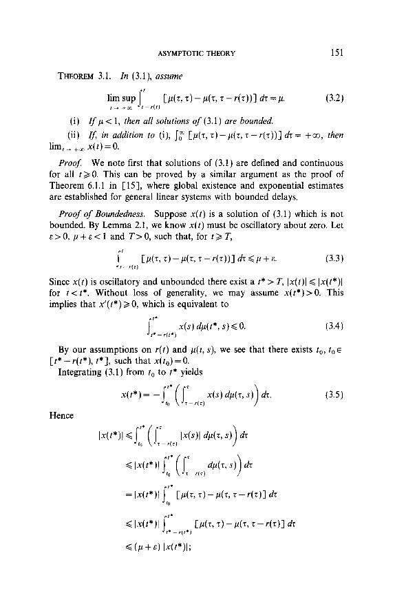
THEOREM 3.1. In (3.1), assume

lim sup 1’ CP(Z, r)- ~(7, r - r(~))l dz = P. (3.2) t- fat I ~ r(t)

(i) If,u< 1, th en all solutions of (3.1) are bounded.

(ii) If, in addition to (i), Jr [~(t, z) -p(r, r--r(z))] dz = +oo, then lim t4 +cc x(t)=O.

Proof: We note first that solutions of (3.1) are defined and continuous for all t > 0. This can be proved by a similar argument as the proof of Theorem 6.1.1 in [ 151, where global existence and exponential estimates are established for general linear systems with bounded delays.

Proof of Boundedness. Suppose x(t) is a solution of (3.1) which is not bounded. By Lemma 2.1, we know x(t) must be oscillatory about zero. Let E>O, p+s<l and T>O, such that, for tbT,

s I bL(r, ~1 -AT, r - r(r))] dz Q ,u + E. f-r(t)

(3.3)

Since x(t) is oscillatory and unbounded there exist a t* > T, Ix(t)1 d Ix(t*)l for t< t*. Without loss of generality, we may assume x(t*) > 0. This implies that x’( t*) > 0, which is equivalent to

I t*

x(s) dp(t*, s) < 0. I*--r(t*)

(3.4)

By our assumptions on r(t) and ,u(t, s), we see that there exists t,, to E [t*-r(t*), t*], such that x(t,)=O.

Integrating (3.1) from t, to t* yields

Hence

= Ix(t*)l 1,: CP(G z)- ,4~, 7 - r(r)1 dr

< lx(t*)l I” [At, r)- P(G 7 - r(t)1 dr t* - r(t*)

(3.5)

G b+ 6) Idt*)l;

152 HADDOCKANDKUANG

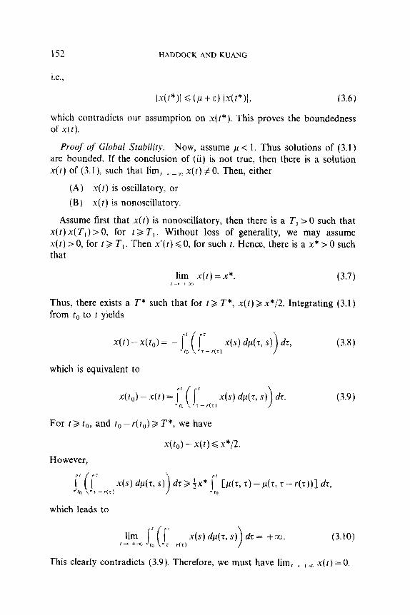
i.e..

Idf*)l < (PL+ F) I-4t*)/, (3.6)

which contradicts our assumption on x(t*). This proves the boundedness of x(r).

Proof qf Global Stability. Now, assume p < 1. Thus solutions of (3.1) are bounded, If the conclusion of (ii) is not true, then there is a solution x(t) of (3.1) such that lim,, +X x(t) f-0. Then, either

(A) x(t) is oscillatory, or (B) x(t) is nonoscillatory.

Assume first that x(t) is nonoscillatory, then there is a T, > 0 such that x(t) x(T,) > 0, for t b T,. Without loss of generality, we may assume x(t) > 0, for t > T, . Then x’(t) < 0, for such t. Hence, there is a x* > 0 such that

lim x(t) =x*. (3.7) ,- +m

Thus, there exists a T* such that for t b T*, x(t) > x*/2. Integrating (3.1) from t, to t yields

x(t) - x(tcJ = -jr ( j;-,,,, 4s) dl*(r,s)) & 10 which is equivalent to

x(b) -x(t) = j’ ( j;p,,r, 4s) d/47,4) d7. 10

(3.8)

(3.9)

For rB to, and to--(to)8 T*, we have

x(to) - x(t) d x*/2,

However,

x(s)dp(r,s))dr>jx* jt; C/47> 7) - c~(c7 - r(7))l d7,

which leads to

, 7 lim

J (J x(s) dp(7, s) d7 = +a. (3.10)

t-+5 to T--r(?) >

This clearly contradicts (3.9). Therefore, we must have lim,, +r* x(t) = 0.

ASYMPTOTIC THEORY 153

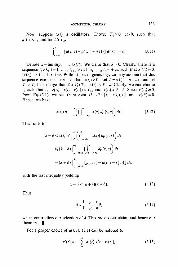
Now, suppose x(t) is oscillatory. Choose T2 > 0, E > 0, such that P+E< 1, and for t> T2,

s I [P(T, 7)-/d? T-r(T))] d-P++. (3.11) f-l(f)

Denote X = lim sup, _ +ao Ix(t)l. We claim that X=0. Clearly, there is a sequence ti > 0, i = 1,2, . . . . ti+ I > ti, lim,, +m ti = + co, such that x’(ti) = 0, Ix(ti)J -+X as i-+ +co. Without loss of generality, we may assume that this sequence can be chosen so that x(t;) > 0. Let 6 = 4x( 1 -p - E), and let T, > T2 be so large that, for t 3 T3, Ix(t)/ < X + 6. Clearly, we can choose t, such that ti - r( ti) - r( ti - r( ti)) > T3, and x( t,) > X - 6. Since x’( ti) = 0, from Eq. (3.1), we see there exist t*, t*E [ti-r(t,), ti] and x(t*)=O. Hence, we have

This leads to

=(X+8) f, s b(T, T) - P(G T-r(T))] & f, - e&l with the last inequality yielding

Thus,

6> l-p-E2 l+p+E ’

(3.12)

(3.13)

(3.14)

which contradicts our selection of 6. This proves our claim, and hence our theorem. 1

For a proper choice of ,u(t, s), (3.1) can be reduced to

x’(t)= - i a,(t)x(t-r,(t)), i=O

(3.15)

154 HADDOCKANDKUANG

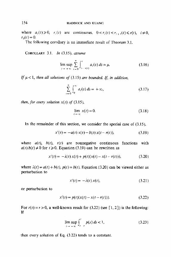
where a,(t) 2 0, r,(t) are continuous, O<r,(t)<ri+l(t)~r(‘t), if0, r,(t) = 0.

The following corollary is an immediate result of Theorem 3.1.

COROLLARY 3.1. 1~ (3.15), a~ume

lim sup i 1’ a,(s) ds = p. 1- +cc ;=(I r-r(r)

Zf p < 1, then all solutions of (3.15) are bounded. If, in addition,

(3.16)

(3.17)

then, for every solution x(t) of (3.15),

lim x(t) = 0. (3.18) I-Z

In the remainder of this section, we consider the special case of (3.15),

x’(t)= -a(t)x(t)-b(t)x(t-r(t)), (3.19)

where u(t), b(t), r(t) are nonnegative continuous functions with a(t) b(t) # 0 for t > 0. Equation (3.19) can be rewritten as

x’(t)= -Il(t)x(t)+p(t)(x(t)-x(t-r(t))), (3.20)

where A(t) = a(t) + b(t), p(t) = b(t). Equation (3.20) can be viewed either as perturbation to

x’(t) = -A(t) x(t), (3.21)

or perturbation to

x’(t)=p(t)(x(t)-x(t-r(t))). (3.22)

For r(t) = r > 0, a well-known result for (3.22) (see [ 1, 21) is the following: If

5 I

lim sup P(S) ds < 1, (3.23) f- +m I--r

then every solution of Eq. (3.22) tends to a constant.

ASYMPTOTIC THEORY 155

For any t,, > 0, (3.19) is equivalent to

x(r)=exp(ji--a(s)ds) cl

X(l(i”)-~~:exp(~~ii)d*)h(B)X(S--I(SJ)L). (3.24)

If either j; a(s) ds = +oo or j: b(s) ds = +oo, then we see solutions of (3.19) either are oscillatory or tend to zero as t + +co. In the following, we assume x(t) is an oscillatory solution of Eq. (3.19). Let x(t*) be any local maximum of x(t), where t* - r(t*) > 0, then Y(t*)=O. Clearly, Eq. (3.19) implies that x(t* - r(t*)) Q 0. Thus, there is a lo E [t* - r(t*), t*], such that x( to) = 0. For this t,, (3.24) reduces to

x(t) = - 5’ exp (- j’ a(z) dr) b(s) x(s - r(s)) ds, 10 s

(3.25)

which leads to

Ix(t*)l <jr* exp(-~S’*o(r)di)b(s)/x(s-r(s))~ds. (3.25’) 10

By a similar argument as the proof of Theorem 3.1, one can easily show:

THEOREM 3.2. In (3.19), assume a(t), b(t), r(t) are nonnegative con-

tinuous functions with a(t) b(t) # 0 for t > 0. Further, assume

(i) either 12 a(s) ds = +a, or f: b(s) ds = +oo, and

6) lim SUP,, +m jiL(,) exp( --ii a(~) dz) b(s) ds = p < 1.

Then, all solutions of (3.19) tend to zero as t + +CCI.

Proof: We omit the proof to avoid repetition. 1

For Eq. (3.20), Theorem 3.2 implies that if A(t) > P(Z) b 0, (A(t) - p(t)) p(f) Z 0, so” (n(s) - p(s)) ds = +a, and

then all solutions of (3.20) tend to zero as t + +co. This is in contrast to a result obtained in [ 11, where it asserts that SO” A(s) ds < + co, together with (3.23), implies each solution of (3.20) tends to a constant as t + +c.c. Our result indicates that in the following sense the conclusion in [ 1 ] is sharp: If s: p(s) ds< +cc, and f; A.(s) ds< +oo, then each solution of

156 HADDOCKANDKUANG

(3.20) tends to a constant as t -+ +co, while if 1; p(s) ds < +as and jc 1.(s) ds = +x, then all solutions of (3.20) tend to zero, as t + +a.

If all the functions J.(t), p(t), and r(t) appearing in Eq. (3.20) are real constants, then sufficient and necessary conditions can be derived from those general results obtained in [lo] for linear scalar neutral delay equations, which include Eq. (3.20) as a special case.

4. NONLINEAR EQUATIONS

In this section, we return to Eq. (2.1); that is,

(4.1)

The following generalizes Theorem 3.1.

THEOREM 4.1. In (4.1), for c #O, assume jf(z, c)l is nondecreasing with respect to c, and

lim sup s ,l-rl,, cplf(~, ~)CP(L ~1 -AT, 7 - r(~))l dr G p < 1, (4.2) I- tm

then all global solutions of (4.1) are bounded. If, in addition, for c # 0,

s om M-c, c)l IM, 7) - ACT - r(T))1 dz = +a, (4.3)

then all global solutions of (4.1) tend to zero as t -+ +so.

Outline of the Proof: By Lemma 2.1, if a global solution x(t) of (4.1) is not bounded, then it must be oscillatory. By a similar argument as the proof of Theorem 3.1, one can show x(t) must be bounded. The condition (4.3) together with the monotonicity of If(r, c)l (with respect to c) ensures that x(t) cannot tend to a nonzero constant. Thus, x(t) either tends to zero, or is oscillatory. In the latter case, the assumption (4.2) leads to lim r- ix, x(t)=O. 1

Remark 4.1. The above theorem is in contrast to the recent result in [21, Theorem 3.11 where r(t) is assumed to be bounded andf(t, x) satisfies a Yorke Condition (see [20]). Under these two conditions, Theorem 3.1 in [21] is sharper.

Denote t, = min{ t : t = r(t)}. We have the following local result.

ASYMPTOTIC THEORY 157

THEOREM 4.2. Assume, for (4.1), If(r, c)l is nondecreasing with respect to c, and there is an M > 0, such that for )c) < M, we have

(i) s:- r(t) c-‘f(z,c)C~(Z,~)--11(T,~-r(~))]dZ~~<l,

for t>,t,, (4.4)

(ii) jam lf(5 c)l CA r,T)--p(t,r--r(z))]dz= +oo,c#O, (4.5)

(iii) IfIr, c)l G a(z) I4 where a(z) is continuous

and nonnegative for z > 0. (4.6)

Then, for any 0 <E 6 M, there is a B(E) > 0, such that, for 4 E C, 1lq511 < B(E), Ix(t)1 GE and lim,, += x(t) = 0, where x(t) is the solution of (4.1) with initial function 4.

Proof. First, we claim that, for small enough 6 > 0, if \I~$11 < 6, then x(t), the solution of (4.1) with initial function 4, satisfies Ix(t)1 CM, for tE co, &)I.

Integrating (4.1) from 0 to t, leads to

x(t) = 40) - j’ ( j’ (4.7) 0 7 - r(r)

f(T, x(s)) &(c 4) d?.

Assume Ix(s)1 6 M, for s E C-r, to], where r = r(0). By assumption (iii), we have

Ill G I.@)l + 1: (j:- I(T) a(z) Ill &Cc $1) dz.

Let Z(t)=max{Ix(s)l;s~[-r, t]}, then (4.8) leads to

(4.8)

T(t) <Z(O) + \i Z(z) a(z)[p(z, o) - p(z, ~-r(s))] dt.

Thus, by Gronwall’s inequality, we have

-f(t) <-f(O) exp 1: a(z)Cp(z, T)- ~(7, T - r(z))1 dt (4.9)

Hence, if we choose Z(O) < 6, where

6=Mexp - {J

lo Alma, T)- 4~ 7 - 4~))l dz , (4.10) 0

then 1x( t)l < Xj t) < M, for t E [0, to], proving the claim.

409/168/l-11

158 HADDOCK AND KUANG

In the following, we prove that for any 0 <F d M, we can choose

C?(E) = t: exp d~)bL(c 7) -A? T -r(z))] dz , i

(4.11)

such that for I/#11 <6(e), /.~(t)l <E, and lim,, +X x(t) = 0. Clearly, by the proof of the above claim, we have Ix(t)1 < E for t E [0, t,].

Assume there is a t* 2 t,, such that for s 6 t*, Ix(s)l GE, x(t*) = E, and x’(t*)>O (the case of x(t*)= -a, x’(t*)<O can be dealt with similarly). Then, Eq. (4.1) indicates there is a t’c [t*-r(t*), t*] such that x(t’)=O. Clearly, t* - r( t*) 2 t, - Y( to) = 0. We have

& = Ix(r*)l 6 lf(r, x(s))1 447, s) (4.12)

By the monotonicity of jf(z, x)1, we have

(4.13)

which leads to

i

1* E~~~(~,E)[~~(~,z)--(z,z--Y(~))I dT>l, (4.14)

f’ -r(P)

a contradiction to assumption (i). The rest of the proof is similar to the proof of Theorem 4.1; we omit the

details here. 1

In particular, for equation

x’(t)= -cr(t)xyt-r(t)), (4.15)

where y > 0 is the quotient of odd integers, we have the following result. For stability definitions, see [ 151.

COROLLRY 4.1. In (4.15), assume y> 1, cc(t) and r(t) are positive continuous, and t - r(t) is nondecreasing. Then, the following statements are true:

(i) ?f

5 t

lim sup a(s) ds < +CO, r-r(r)

(4.16)

then the zero solution is uniformly stable.

ASYMPTOTIC THEORY 159

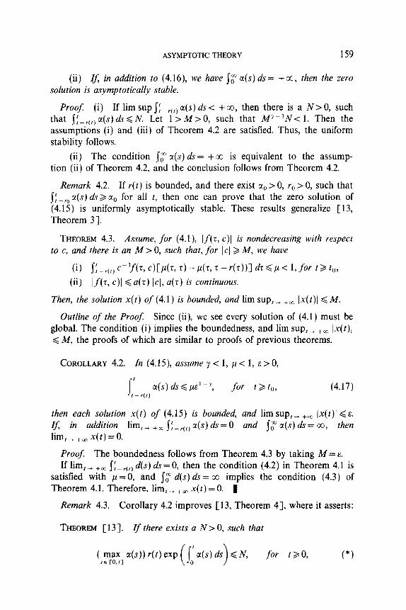
(ii) If, in addition to (4.16), we have 1: a(s) ds= +CC, then the zero solution is asymptotically stable.

Proof (i) If lim sup J:Pr(tJ a(s) ds < + co, then there is a N> 0, such that j:-r(,J U(S) ds< N. Let 1 >M>O, such that MY-IN< 1. Then the assumptions (i) and (iii) of Theorem 4.2 are satisfied. Thus, the uniform stability follows.

(ii) The condition JO” LX(S) ds = +co is equivalent to the assump- tion (ii) of Theorem 4.2, and the conclusion follows from Theorem 4.2.

Remark 4.2. If r(t) is bounded, and there exist CI~ > 0, r0 > 0, such that J:-, M(S) ds 2 ~1~ for all t, then one can prove that the zero solution of (4.15) is uniformly asymptotically stable. These results generalize [ 13, Theorem 31.

THEOREM 4.3. Assume, for (4.1), If(z, c)l is nondecreasing with respect to c, and there is an M > 0, such that, for IcJ > M, we have

(i) I:-r(,) c-‘f(~ ~)CP(G z1-A~ z-r(z))1 dT,<p< L&r tBto, (ii) If(r, c)l Q a(z) /cl, a(z) is continuous.

Then, the solution x(t) of (4.1) is bounded, and lim supr- +m Ix(t)1 GM.

Outline of the Proof: Since (ii), we see every solution of (4.1) must be global. The condition (i) implies the boundedness, and lim sup,, +lo Ix(t)/ < M, the proofs of which are similar to proofs of previous theorems.

COROLLARY 4.2. In (4.15), assume y < 1, p < 1, E > 0,

I I

cc(s)ds+~-~, for tat,, I-r(t)

(4.17)

then each solution x(t) of (4.15) is bounded, and lim sup,+ +m (x(t)1 <E. If, in addition lim,, +aj j:-,([, c~(s)ds=O and jr a(s) ds= co, then lim t--t +m x(t)=@

Proof The boundedness follows from Theorem 4.3 by taking M = E. If lim I--r +ao j:-lc,, d(s) ds= 0, then the condition (4.2) in Theorem 4.1 is

satisfied with ~1 =O, and j; d(s) ds = cc implies the condition (4.3) of Theorem 4.1. Therefore, lim, j + a3 x(t) = 0. 1

Remark 4.3. Corollary 4.2 improves [13, Theorem 41, where it asserts:

THEOREM [ 131. Zf there exists a N> 0, such that

(sz;, a(s)) r(t) exp (1: a(s) ds) <N, for t > 0, (*)

160 HADDOCKANDKUANG

then all solutions of (4.15) are bounded. If, in addition, s; a(t) dt = 00, then all solutions tend to zero as t -+ + xj.

Clearly, if (*) is satisfied, then

s I a(s)ds<( max C((s))r(t)<N. r-r(r) J E co, r1

Hence (4.17) is satisfied with E’-? = N/p, and thus all solutions of (4.15) are bounded. If, in addition, j; a(t) dt = co, then (*) implies jiPr(,) M(S) ds -+ 0, as t + +co. Therefore, by Corollary 4.2, we conclude that all solutions of (4.15) tend to zero as t -+ + a.

In the rest of this section, we consider

,y’ = - i ai(t)(ex(‘-“(‘)) - I), i= I

(4.18)

where a;(t), ri( t) are nonnegative and continuous, r(t) = max{ ri( t) : i = 1, . . . . n} > 0. It is equivalent to

Y’= - i ai( 1) At-r,(t)),

i=l

(4.19)

and can be further reduced to the general delay logistic equation of the form

z’(t)=R(t)z(t) [

l-Ccli(t)z(t-r,(t)) , 1

(4.20)

where Cr= i q(t) = 1, and R(t) 3 0. By applying Theorem 4.2 to (4.18), we can obtain the following

asymptotical stability result.

COROLLARY 4.3. In (4.18), assume there is a M>O, such that

(ii) jgl Jr a,(s) ds= +a.

Then, for any 0 <E < M, there is a 8(c) > 0, such that, for 4 E C, 11411 < 6(~), we have Ix(t)1 GE and lim,, +lo x(t) = 0. Here x(t) is the solution of (4.18) with initial function 4.

ASYMPTOTIC THEORY 161

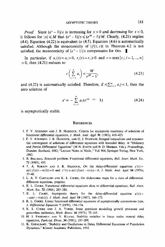
Pro05 Since (ex - 1 )/x is increasing for x > 0 and decreasing for x < 0, it follows for 1x1 <M that (ex- 1)/x< (e”- 1)/M. Clearly, (4.21) implies (4.4). Equation (4.22) is equivalent to (4.5). Equation (4.6) is automatically satisfied. Although the monotonicity of If(z, c)l in Theorem 4.2 is not satisfied, the monotonicity of (e-’ - 1 )/x compensates for this. 1

In particular, if a,(t)=ai>O, r,(t) = ri>O and r=max(ri; i= 1, . . . . H} > 0, then (4.21) reduces to

(4.23)

and (4.22) is automatically satisfied. Therefore, if r(C?=, ai) < 1, then the zero solution of

x’= - i ai(ex(rp”‘- 1) (4.24) i=l

is asymptotically stable.

REFERENCES

1. F. V. ATKINSON AND J. R. HADDOCK, Criteria for asymptotic constancy of solutions of functional differential equations, J. Math. Anal. Appl. 91 (1983), 410-423.

2. F. V. ATKINSON, J. R. HADDOCK, AND 0. J. STAFFANS, Integral inequalities and exponen- tial convergence of solutions of differential equations with bounded delay, in “Ordinary and Partial Differential Equations” (W.N. Everitt and B. D. Sleeman, Eds.), Proceedings, Dundee, Scotland, 1982; “Lecture Notes in Math.,” Vol. 964, Springer-Verlag, New York, 1982.

3. R. BELLMAN, Research problem: Functional differential equations, Bull. Amer. Math. Sot. 71 (1965), 495.

4. T. A. BURTON AND J. R. HADDOCK, On the delay-dilTerentia1 equations x’(r) + a(f)f(x(t-r(f)))=0 and x”(t)+a(f)f(x(r-r(t)))=O, J. Math. Anal. Appl. 54 (1976), 3748.

5. L. A. V. CARVALHO AND K. L. COOKE, On dichotomic maps for a class of differential- difference equations, preprint.

6. K. L. COOKE, Functional differential equations close to differential equations, Bull. Amer. Math. Sot. 72 (1966), 285-288.

7. K. L. COOKE, Asymptotic theory for the delay-differential equation u’(t) = -au(r-r(u(r))), J. Mafh. Anal. Appl. 19 (1967), l&173.

8. K. L. COOKE, Linear functional differential equations of asymptotically autonomous type, J. Dif,ferential Equations 7 (1970), 154174.

9. K. I,. COOKE AND J. A. YORKE, Some questions modelling growth processes and gonorrhea epidemics, Math. Biosci. 16 (1973), 75-101.

10. H. I. FREEDMAN AND Y. KUANG, Stability switches in linear scalar neutral delay equations, Funkcial. Ekuac. 34 (1991), 187-209.

11. K. GOPALSAMY, “Stability and Oscillations in Delay Differential Equations of Population Dynamics,” Kluwer Academic Publishers, 1992.

162 HADDOCKANDKUANG

12. S. E. GROSSMAN AND J. A. YOKKE. Asmptotic behavior and exponential stability criteria for differential delay equations, J. D$firen/ial Equations 12 (1972), 236-255.

13. J. R. HADDOCK, On the asymptotic behavior of solutions of .x’(l) = -u(r)f(x(~ - r(t))), SIAM J. Math. Anal. 5 (1974), 569-573.

14. J. R. HADDOCK AND J. TERJBKI, Liapunov-Razumikhin functions and an invariance principle for functional differential equations, J Dijjferenfial Equations 48 (1983), 95-122.

15. J. K. HALE, “Theory of Functional Differential Equations,” Springer-Verlag, New York, 1977.

16. J. KAPLAN, M. SORG, AND J. YORKE, Solutions of .x’(t)=,[(x(t), ~(t-L)) have limits when f is an order relation, Nonlinear Anal. 3 (1979), 53-58.

17. G. L. SLATER, The differential-difference equation W’(S) = g(s)[w(s- 1) -M.(S)], Proc. Roy. Sot. Edinburgh Seer. A 18 (1977), 41-55.

18. T. YONEYAMA, On the 3/2 stability theorem for one-dimensional delay-differential equations, J. Math. Anal. Appl. 125 (1987), 161-173.

19. T. YONEYAMA, Exponentially asymptotically stable dynamical systems, Appl. Anal. 27 (1988), 235-242.

20. T. YONEYAMA AND J. SUGIE, On the stability region of differential equations with two delays, Funkciul. Ekunc. 31 (1988), 233-240.

21. T. YONEYAMA AND J. SUGIE, Perturbing uniformly stable nonlinear scalar delay-differential equations, Nonlinear Anal. 12 (1988), 303-311.

22. J. A. YORKE, Asymptotic stability for one dimensional differential-delay equations, J. Differential Equations 7 (1970), 189-202.