Lyapunov’s Second Method for

Nonautonomous Differential Equations∗

September 26, 2006

Lars Grune

Mathematisches InstitutUniversitat Bayreuth

95440 Bayreuth, Germany

Peter E. Kloeden and Stefan Siegmund

Institut fur Computerorientierte MathematikJ.W. Goethe Universitat

60054 Frankfurt, Germany

Fabian R. Wirth

The Hamilton InstituteNational University of Ireland Maynooth

Maynooth, Co. Kildare, Ireland

(Communicated by Aim Sciences)

Abstract

Converse Lyapunov theorems are presented for nonautonomous sy-

stems modelled as skew product flows. These characterize various types

of stability of invariant sets and pullback, forward and uniform attractors

in such nonautonomous systems.

MSC subject classification: 37B25, 37B55, 93D30

Keywords: Lyapunov function, Lyapunov’s second method, nonautonomousdynamical system, nonautonomous differential equation, stability, nonautono-mous attractor.

∗Peter Kloeden was partially supported by the Ministerio de Educacion y Ciencia in Spainunder the Programa de Movilidad del Profesorado universitario espanol y extranjero, grantSAB2004-0146. Stefan Siegmund was supported by the Emmy Noether program of the DFG.Fabian Wirth acknowledges support by the Science Foundation Ireland grants 04-IN3-I460and 00/PI.1/C067.

1

1 Introduction

Asymptotic stability is one of the corner stones of the qualitative theory ofdynamical systems and is of fundamental importance in many applications of thetheory in virtually all fields where dynamical effects play a role. In the analysisof stability properties of invariant objects it is very often useful to employ whatis now called Lyapunov’s second method [4] (see [2] for a random version). Thismethod relies on the observation that asymptotic stability is intimately linkedto the existence of a Lyapunov function, that is, a proper, nonnegative function,vanishing only on an invariant set and decreasing along those trajectories of thesystem not evolving in the invariant set. Lyapunov proved that the existenceof a Lyapunov function guarantees asymptotic stability and for linear time-invariant systems also showed the converse statement that asymptotic stabilityimplies the existence of a Lyapunov function. Converse theorems usually arethe harder part of the theory and the first general results for nonlinear systemswere obtained by Massera [22, 23] and Kurzweil [18, 19]. Converse theorems areinteresting because they show the universality of Lyapunov’s second method.If an invariant object is asymptotically stable then there exists a Lyapunovfunction. Thus there is always the possibility that we may actually find it,though this may be hard.

A typical direct and converse result is the following found in Bhatia andSzego [4, Theorem V.2.12].

Theorem 1. Let ϕ be a topological dynamical system on a locally compactspace X, and let A be a nonvoid compact set which is invariant under ϕ.

Then A is asymptotically stable if and only if there exists a Lyapunov func-tion for A, i.e. a function V : X → R

+ such that

(i) V is continuous,

(ii) V is uniformly unbounded, i.e. for all C > 0 there exists a compact setK ⊂ X such that V (x) ≥ C for all x 6∈ K,

(iii) V is positive-definite, i.e. V (x) = 0 if x ∈ A, and V (x) > 0 if x 6∈ A,

(iv) V is strictly decreasing along orbits of ϕ, i.e. V (ϕ(t, x)) < V (x) for x 6∈ Aand t > 0.

Furthermore, V can be chosen to satisfy

V (ϕ(t, x)) = e−tV (x) for all x ∈ X, t ∈ R.

Despite the considerable time and effort that has been spent on developingstability theory, important progress has still been made with respect to thetheory of Lyapunov functions in recent times. Probably the most far-reachingextension is Conley’s work on global Lyapunov functions with respect to Morsesets of a dynamical system that allows a precise characterization of the system’sglobal behavior [9, 7, 8]. Secondly, for systems in R

d several results have beenobtained that show the existence of smooth Lyapunov functions under minimal

2

assumptions on the regularity of the differential equation [29, 24, 21]. Con-structive methods to find Lyapunov functions numerically for arbitrary systems(methods that are usually feasible in low dimensions) have been presented in[32, 6, 13].

Finally, the question of whether the rate of attraction can be recovered by anappropriate choice of a Lyapunov function has been shown for different systemclasses in [11, 30]. The latter fact has been known for linear time invariantsystems since the work of Massera, [22, 23]. One approach to describe attractionrates for general nonlinear systems relies on so-called comparison functions. Thisapproach goes back at least to Hahn [14] and has been popularized again in thepast decade by influential works as [26, 15].

In this paper we study the problem of converse Lyapunov theorems for non-autonomous dynamical systems. The asymptotically stable objects are given na-turally by pullback, forward and uniform attractors. We prove converse Lyapu-nov theorems for these attractor types. The focus of the paper lies on obtainingLyapunov functions that recover certain attraction rates given in terms of com-parison functions, that is functions of class K and class KL. To this end weshow how the different notions of stability and attractivity that play a role wi-thin the nonautonomous framework can be characterized in terms of attractionrates given by comparison functions. We then show that the existence of anattraction rate in terms of comparison functions is equivalent to the existenceof a Lyapunov function guaranteeing this attraction rate. We note that forhyperbolic skew product flows some Lyapunov theory is available in [5].

The paper is organized as follows: In the following Section 2 we introducethe formalism of skew product flows and nonautonomous sets. Invariant objectswill be found in this class. In Section 3 we define several notions of stabilityand attractivity of invariant nonautonomous sets. In particular, the notions ofpullback, forward and uniform attractors are defined. For the proofs to come itturns out to be vital that the notions of attractor is defined with respect to theattraction of arbitrary compact sets. We comment on this and show that thisimplies stability properties as well. In Section 4 Lyapunov functions are definedand it is shown that if the base space of the skew product flow is compact,then only maximal invariant sets can possess Lyapunov functions. In Section 5we first show that a skew product flow satisfies a decay condition expressed interms of comparison functions if and only if there exists a Lyapunov functioncharacterizing this decaying behavior. The next step is obtained in Section 6,where it is shown how the different notions of stability and attractivity maybe equivalently expressed in terms of nonautonomous comparison functions.The section starts with a case study to highlight the various phenomena thatcan occur within this theory. The main result of the section is obtained inSubsection 6.2. The final result in Subsection 6.3 then provides Lyapunov andconverse Lyapunov theorems for the various stability notions of interest for skewproduct flows.

Notation: The open ball in Rd of radius ε centered at x is denoted by Bε(x)

and its closure is denoted Bε(x). For x ∈ Rd and a closed nonempty set A we

3

define the distance of x to A by

‖x‖A := min{ ‖x − y‖ | y ∈ A} .

For non-empty closed sets A and B the Hausdorff semi-metric d(A|B) is definedby

d(A|B) := sup{ ‖x‖B | x ∈ A} .

So d(A|B) measures how far A is from B (d(A|B) = 0 only implies that A ⊆ B),while

dH(A,B) := d(A|B) + d(B|A)

denotes the Hausdorff metric.

2 Skew Product Flows and Nonautonomous Sets

The concept of skew product flows arose from topological dynamics during the1960s as a description of dynamical systems with “nonautonomy”, i.e. showingan explicit dependence on the actual time rather than just on the elapsed timeas in autonomous systems. Since then, skew product flows have extensively beenstudied, [5, 3, 12, 17, 28]. They are tailor-made to nonautonomous systems suchas nonautonomous differential equations

x = f(t, x) .

We do not obtain a dynamical system directly from solving the respective dif-ferential equation. Instead, the solution gives rise to a so-called cocycle over adynamical system which models the nonautonomy of the equation.

Here is a formal definition, where for the sake of not overburdening thepresentation we restrict ourselves to the case of a state space R

d and continuoustwo-sided time R.

Definition 2 (Skew Product Flow (SPF)). A skew product flow , shortly deno-ted by ϕ, consists of two ingredients:

(i) A model of the nonautonomy, namely a continuous dynamical systemθ : R × P → P , where P is a complete metric space.

(ii) A model of the system perturbed or forced by nonautonomy, namely acocycle ϕ over θ, i.e. a continuous mapping ϕ : R × P × R

d → Rd, (t, p, x) 7→

ϕ(t, p, x), such that the family ϕ(t, p, ·) = ϕ(t, p) : Rd → R

d of self-mappings ofR

d satisfies the cocycle property

ϕ(0, p) = idX , ϕ(t + s, p) = ϕ(t, θ(s)p) ◦ ϕ(s, p) , (1)

for all t, s ∈ R and p ∈ P .

4

The pair of mappings

(θ, ϕ) : R × P × Rd → P × R

d , (t, p, x) 7→ (θ(t, p), ϕ(t, p, x)) ,

is called the corresponding skew product. If P = {p} consists of a single point,then the cocycle ϕ is a dynamical system on R

d. We often use the less clumsynotation θt instead of θ(t). The well-known trick of making a nonautonomousdifferential equation

x = f(t, x) (2)

autonomous by introducing a new variable for the time suggests to investigate acorresponding skew product flow with base P := R and driving system (t, s) 7→θts := t+s. However, as P does not depend on f , we should not expect a specifickind of nonautonomy (e.g. periodicity in t) to be captured by this base dynamics.Moreover, P is not compact which may cause additional difficulties. For a fairlygeneral class of right hand sides f the Bebutov flow (t, p) 7→ θtp := p(·+ t, ·) onthe hull P := H(f) = cl{f(· + t, ·) : t ∈ R} of f can serve as a model for thenonautonomy (Sell [25]). Here the closure is taken with respect to an adequatetopology. The evaluation mapping

f : P × Rd → R

d, (p, x) 7→ p(0, x)

satisfies f(θtp, x) = p(t, x) and, since f ∈ H(f) and therefore f(θtf, x) = f(t, x),it is a natural “extension” of f to P × R

d. As a slight abuse of notation wewill sometimes omit the bar. Instead of looking at the single equation (2) weconsider the associated family of equations

x = f(θtp, x), p ∈ P = H(f). (3)

By using standard results about linearly bounded equations as in Amann [1]and Arzela-Ascoli’s theorem the following may be shown, [3].

Theorem 3 (SPF from Nonautonomous Differential Equation). Let f : R ×R

d → Rd be a continuous function, and consider the nonautonomous differential

equation (2). If (t, x) 7→ f(t, x) is locally Lipschitz in x and

‖f(t, x)‖ ≤ α(t)‖x‖ + β(t) ,

where t 7→ α(t) and t 7→ β(t) are locally integrable, then the hull P := H(f) isa metric space (where the closure is taken in C(R × R

d, Rd) with the compact-open topology), the Bebutov flow (t, p) 7→ θtp = p(·+ t, ·) is continuous, and (2)uniquely generates an SPF ϕ over θ through the solution

ϕ(t, p, x) = x +

∫ t

0

f(θsp, ϕ(s, p, x)) ds (4)

of the associated family of equations (3). Moreover, H(f) is compact if andonly if (t, x) 7→ f(t, x) is bounded and uniformly continuous on every set of theform R × K where K ⊂ R

d is compact.

5

We now turn to the concepts we need in order to be able to define attractorsfor nonautonomous systems. In general, there is no reason to assume thatthese should be autonomous objects themselves. The following notion of setsdepending on the parameter p is standard.

Definition 4 (Nonautonomous Set). A function M : p 7→ M(p) taking valuesin the non-empty closed/compact/bounded subsets of R

d is called a nonauto-nomous closed/compact/bounded set.

For convenience we will often suppress the p argument of M . The set M(p)is called the p fibre of the nonautonomous set M . In general the term p fibre ofan expression will be used in discussing the expression for the specific parametervalue p.

Definition 5 (Invariance of Nonautonomous Set). A nonautonomous set Mis called forward invariant under the SPF ϕ if ϕ(t, p,M(p)) ⊂ M(θtp) for allt ≥ 0. It is called invariant if ϕ(t, p,M(p)) = M(θtp) for all t ∈ R.

3 Asymptotic Stability of Nonautonomous Sets

Asymptotic stability is usually defined through the properties of stability andattractivity. For nonautonomous attractors, there are various ways to definestability, as well as attraction. We present some of the standard definitionshere.

The following notion of stability is taken from [20, Definition 2.3].

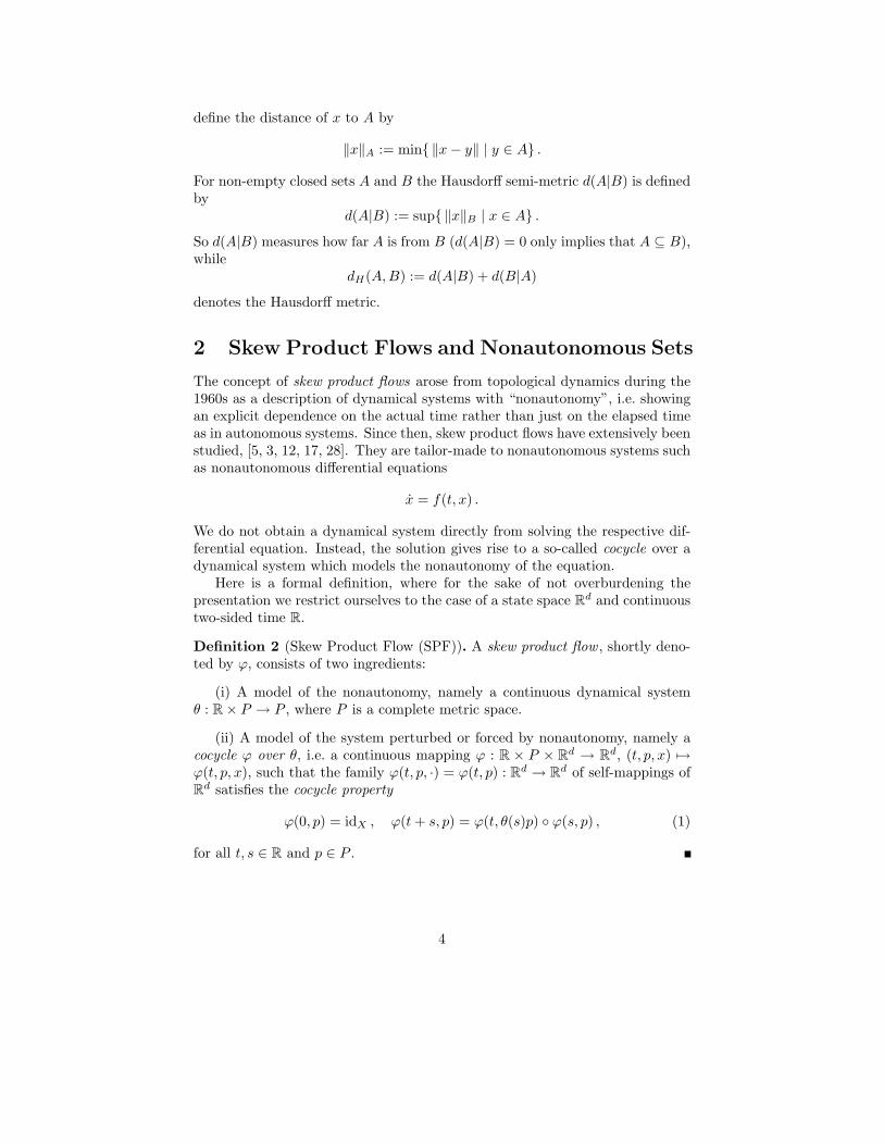
Definition 6 (Pullback Stability). Let ϕ be an SPF and A be a nonautonomouscompact set invariant under ϕ. Then A is called (pullback) stable under ϕ if forany ε > 0 there exists a function p 7→ δε(p) > 0 such that for any x ∈ R

d, p ∈ Pthe relation d(x,A(θ−tp)) ≤ δε(p) implies that d(ϕ(t, θ−tp, x), A(p)) ≤ ε for anyt ≥ 0.

If, in addition, δε may be chosen so that for each p ∈ P we have δε(p) → ∞as ε → ∞, then A is called globally (pullback) stable.

The next definition is inspired by [2, Definition 4.1]. We recall that a compactset C ⊂ R

d is called a neighborhood of A ⊂ Rd if A ⊂ int C. Similarly, a

nonautonomous compact set C is a neighborhood of A, if C(p) is a neighborhoodof A(p) for all p ∈ P .

Definition 7 (Forward Stability). Let ϕ be an SPF and A be a nonautonomouscompact set invariant under ϕ. Then A is called (forward) stable under ϕ if forany ε > 0 there exists a nonautonomous compact set C which is a neighborhoodof A such that

(i) dH(C(p), A(p)) ≤ ε for each p ∈ P , i.e. C is ε-close to A,

(ii) ϕ(t, p, C(p)) ⊂ C(θtp) for all t ≥ 0, p ∈ P , i.e. C is forward invariant.

We note the following property implied by Definition 6 for further reference.

6

pθ−tp p

A

δε(p)

δε(p)

ε

εϕ(·, θ−tp, x)

x

x

Figure 1: A is pullback stable, i.e. if x (in the θ−tp-fibre) is δε(p)-close to Athen ϕ(t, θ−tp, x) (in the p-fibre) is ε-close to A.

Lemma 8. Let ϕ be an SPF and A be a nonautonomous compact set whichis invariant under ϕ and pullback stable. Then there exists a bounded forwardinvariant, nonautonomous set C, such that for every p ∈ P there exists η(p) > 0with Bη(p)(A(θ−tp)) ⊂ C(θ−tp) for all t ≥ 0.

Proof. It is sufficient to prove the result along a fixed orbit Γ of θ. Fix ε >0, p ∈ Γ. By definition, there exists a constant δ = δ(p) > 0 such that

ϕ(t, θ−tp,Bδ(A(θ−tp))) ⊂ Bε(A(p)) , for all t ≥ 0 . (5)

If p is a fixed point of θ, i.e. Γ = {p}, the result is standard in the theory ofnonautonomous differential equations. If t 7→ θtp is periodic with period T > 0,define

C(p) :=∞⋃

k=0

ϕ(kT, p,Bδ(A(p))) =∞⋃

k=0

ϕ(kT, θ−kT p,Bδ(A(θ−kT p))) .

Then ϕ(T, p, C(p)) ⊂ C(p), Bδ(A(p)) ⊂ C(p) and by (5) C(p) ⊂ Bε(A(p)), be-cause every point in C(p) is contained in a set of the form ϕ(kT, θ−kT p,Bδ(A(θ−kT p))).For t ∈ [0, T ) we now define

C(θtp) := ϕ(t, p, C(p)) ,

and it follows that C has all the desired properties on Γ. Note that we maydefine η on Γ uniformly as

η :=1

2sup{γ > 0 | Bγ(A(q)) ⊂ C(q) for all q ∈ Γ} .

7

pp θtp

AC

ε

ε

ϕ(·, p, x)

x

x

Figure 2: A is forward stable, i.e. there exists an ε-close forward invariantneighborhood C of A.

Assume now that t 7→ θtp is not periodic. Then we define for t ≥ 0

C(θ−tp) :=⋃

τ≥0

ϕ(τ, θ−t−τ , Bδ(A(θ−t−τp))) .

Then for 0 ≤ s ≤ t we have ϕ(s, θ−tp,C(θ−tp)) ⊂ C(θ−t+sp), Bδ(A(θ−tp)) ⊂C(θ−tp) and using (5) we have C(p) ⊂ Bε(A(p)). By continuity of ϕ this impliesthat all of the sets C(θ−tp), t ≥ 0 are bounded. Finally, we define for t > 0 theset C(θtp) := ϕ(t, p, C(p)). This obviously defines a bounded, forward invariantnonautonomous set C on Γ. For t ≥ 0 we may set η(θ−tp) := δ. To chooseη(θtp) for t ≥ 0 note that for t ≥ 0 we have

0 < µ := sup{γ > 0 | ∀s ∈ [0, t] : Bγ(A(θsp)) ⊂ C(θsp)} < ∞

by the continuity of ϕ, A(p) ⊂ intC(p) and as t is finite. We may thus setη(θtp) := min{δ, µ} . This choice satisfies the assertion by construction.

We now define our notion of attraction, which is based on attraction ofcompact sets.

Definition 9 (Attractor). Let ϕ be an SPF and A a nonautonomous compactset which is invariant under ϕ.

(i) A is called a pullback attractor of ϕ if for every p ∈ P and every compactset D ⊂ R

d

limt→∞

dH(ϕ(t, θ−tp,D), A(p)) = 0

8

(ii) A is called a forward attractor of ϕ if for every p ∈ P and every compactset D ⊂ R

d

limt→∞

dH(ϕ(t, p,D), A(θtp)) = 0

(iii) A is called a uniform attractor of ϕ if for every compact set D ⊂ Rd

limt→∞

dH(ϕ(t, p,D), A(θtp)) = 0 uniformly in p ∈ P.

For introduction and application of pullback attractors, see e.g. [12, 17].

Remark 10. (i) It is easy to see that a uniform attractor is a pullback and aforward attractor. The converse is false in general. An example to this effectcan be given as follows. Let P = [0, 1] and assume that all points in P arefixed points under θ, i.e. θtp ≡ p. We are thus not really dealing with a non-autonomous system, but with a parameterized family of autonomous systems.Consider the differential equation in R given by

x = −px − exp

(−

1

x2

)(px + x(x + 1)2(x − 1)2

).

It is easy to see that the global attractor of the system is given by A(p) = {0},p ∈ (0, 1] and A(0) = [−1, 1]. For p > 0, the set A(p) = {0} is exponentiallyattacting with rate of attraction −p. Hence, the attractor A is not uniform,but of course a pullback and a forward attractor, since there is essentially nodynamics on P .

(ii) Note that in Definition 9 we require attraction of all compact sets as op-posed to attraction of points only. This issue has been discussed for stochasticsystems in [10], from which we cite the following illuminating example. Thetime-invariant system x = x − x3 has the invariant set A := {−1, 0, 1}, whichis a set that attracts all points, but which is not an attractor in the sense ofDefinition 9. The fixed point x∗ = 0 is unstable and so the set A is neitherpullback nor forward stable. Indeed we will show that our definition of attracti-vity has some implications on stability as well. Proposition 11 shows that if theattractor is always contained in a given compact set, then pullback attractionimplies pullback stability. Without any further assumptions forward attractionalways implies forward stability. Example 23 on the other hand shows that itis possible for pullback attractors not to be forward stable and by Example 24forward attractors need not be pullback stable.

(iii) For autonomous and periodic systems (i.e., θT p = p for some T > 0)the definitions of pullback, forward and uniform attractor coincide.

(iv) For some problems it is useful to consider unbounded attracting sets,e.g. for problems in reference tracking. We are forced to assume compact-ness of the attractor for technical reasons in some of the later proofs. Also wenote that our definition of attraction relates this property to the ”‘universe”’ ofbounded sets. It appears reasonable that attractors should also belong to this

9

set. When studying attraction properties of an invariant set A we will thereforeoften assume the existence of a compact set K ⊂ R

d with the property

⋃

p∈P

A(p) ⊂ K . (6)

Otherwise, we would have to consider examples of the following kind:

x = t(x − t) + 1 ,

where the base space is P = R. Clearly, the diagonal {x = t} is an invariantset for the corresponding SPF. It is easy to see that it is a pullback attractor(in fact, the equation is obtained under the transformation x := x + t fromExample 23.)

Note that in the above examples all trajectories below the diagonal are notimportant for attractivity. It appears strange that on ”‘half”’ of the state spacethe system can be altered arbitrarily without any impact on the global attracti-vity properties of the invariant set.

(iv) We note that some care has to be taken, when performing basic ope-rations on the objects we have defined. Clearly, any good stability concept isinvariant under changes of variables. In a time-dependent setting it is natural toallow for time-dependent transformation, but without further conditions, thesemay destroy stability. This is shown by an example in Section 6.1.

Proposition 11. Let ϕ be an SPF and A be a nonautonomous compact setinvariant under ϕ.

(i) If A is a pullback attractor and⋃

p∈P A(p) is bounded, then A is pull-back stable.

(ii) If A is a forward attractor, then it is forward stable.

Proof. (i) Assume that A is a pullback attractor that is not pullback stable.Then there exist an ε > 0 and a p ∈ P such that for all n ≥ 1 there existxn ∈ R

d and tn ≥ 0 with

d(xn, A(θ−tnp)) ≤

1

n, and d(ϕ(tn, θ−tn

p, xn), A(p)) ≥ ε . (7)

By boundedness of⋃

p∈P A(p), the sequence {xn}n∈N is bounded and we may

assume that limn→∞ xn =: x∗ ∈ Rd exists. Furthermore, we may choose η > 0

such that ‖xn‖ ≤ η holds for all n ∈ N. Then by assumption there exists aT > 0 such that for all t ≥ T we have

dH(ϕ(t, θ−tp,Bη(0)), A(p)) ≤ε

2.

This implies for all n ≥ 1 that tn ≤ T and so t∗ := limn→∞ tn may be assumedto exist. Now the invariance of A(θtp) and the continuity of ϕ(t, θtp, x) in timplies that A(θtp) is continuous in t (although A(p) might not be continuous

10

in p). Thus from the first inequality in (7) we obtain x∗ ∈ A(θ−t∗p) while thesecond inequality in (7) implies ϕ(t∗, θ−t∗p, x∗) /∈ A(p). This contradicts theinvariance of the attractor.

(ii) Fix ε > 0 and p ∈ P . We assume that A is a forward attractor. To proveforward stability it is sufficient to prove the existence of the sets C(p) satisfying(i) and (ii) of Definition 7 for a single orbit {θtp | t ∈ R}, as the requirementsfor the overall compact set C only relate to particular orbits. So pick p ∈ P anddefine

C(p) := Bε(A(p)) .

By forward attraction there exists a T ≥ 0 such that for all t ≥ T we have

dH(ϕ(t, p, C(p)), A(θtp)) ≤ε

2.

Define

C(p) := C(p) \ {x ∈ Rd | ∃s ∈ [0, T ] : d(ϕ(s, p, x), A(θsp)) > ε} ,

and C(θtp) := ϕ(t, p, C(p)) for t ≥ 0 (or for t ∈ [0, Tp) if θtp is periodic withperiod Tp).

Then it is easy to see that C(p) is compact and A(p) ⊂ C(p). Indeed, A(p) ⊂int C(p) because otherwise we easily obtain a contradiction to the continuity ofϕ. It follows that for all t ≥ 0 we have A(θtp) ⊂ int C(θtp) and conditions (i)and (ii) of Definition 7 are satisfied. If θtp is not periodic, it remains to extendthe construction to negative t. This can be done inductively. Assume we havedefined C(θtp) for all t ∈ [−n,∞). Then we set

C(θ−(n+1)p) := ϕ(−1, θ−np,C(θ−np)) ,

and

C(θ−(n+1)p) := C(θ−(n+1)p)\{x ∈ Rd | ∃s ∈ [−(n+1),−n] : d(ϕ(s, p, x), A(θsp)) > ε} .

We now set C(θ−(n+1)+sp) := ϕ(s, θ−(n+1)p,C(θ−(n+1)p)) for s ∈ (0, 1), so thatC(θtp) is now defined on [−(n + 1),∞). By the same arguments as before,it follows that the sets C(θtp) satisfy all necessary conditions on the interval[−(n + 1),∞). This shows the assertion.

Definition 12 (Asymptotic Stability). Let ϕ be an SPF and A a nonautono-mous compact set which is invariant under ϕ. Then A is called asymptoticallystable if it is stable and an attractor.

We note that the above definition is a bit loose, as we have to distinguishbetween the six notions of asymptotic stability that can be obtained by com-bining the two notions of stability with the three notions of attractivity. Wewill use the appropriate wording to distinguish between these notions wherenecessary.

11

4 Lyapunov Functions for Skew Product Flows

We now introduce Lyapunov functions with respect to stability and global at-tractivity of a compact invariant set. It is also shown that for compact P aLyapunov function determines a maximal invariant set.

Definition 13 (Lyapunov function). Let ϕ be an SPF in Rd and A be a non-

autonomous compact set which is invariant under ϕ. A family of functions{Vp : R

d → Rd}p∈P is called a Lyapunov function for A (with respect to ϕ) if

it has the following properties:

(i) V is uniformly unbounded, i.e. lim‖x‖→∞ Vp(x) = ∞ for all p ∈ P ;

(ii) V is positive-definite, i.e. Vp(x) = 0 for x ∈ A(p), and Vp(x) > 0 forx 6∈ A(p);

(iii) V is strictly decreasing along orbits of ϕ, i.e.

Vθtp(ϕ(t, p, x)) < Vp(x) for all t > 0 and x 6∈ A(p).

Remark 14. We note that in the previous definition item (i) can be weakenedwithout any harm to the requirement that V be proper, i.e., for all p ∈ Ppreimages of compact sets under Vp(·) should be compact if they are containedin the range of Vp(·). Both approaches to the definition of Lyapunov functionscan be found in the literature.

First we show that Lyapunov functions ensure the uniqueness of invariantnonautonomous compact sets in the following sense.

Proposition 15. Let ϕ be an SPF in Rd and A be a nonautonomous compact

set which is invariant under ϕ. Suppose there exists a Lyapunov function forA. If P is compact, any other invariant nonautonomous compact set A′ satisfiesA′(p) ⊂ A(p) for each p ∈ P .

Proof. Assume the assertion is false, so that there are an invariant nonautono-mous compact set A′, p ∈ P and x ∈ A′(p) \ A(p). By assumption this impliesthat V (p, x) > 0. By compactness of A′ and P and by the unboundedness ofV there is a constant C such that V (q, y) < C for all q ∈ P, y ∈ A′(q). Nowbackwards in time V (θ−tp, ϕ(−t, p, x)) is monotonically increasing and boundedby C due to the invariance of A′. Thus η := limt→∞ V (θ−tp, ϕ(−t, p, x)) exists,and the α-limit set

α(p, x) := {(q, y) ∈ P × Rd | ∃tk → ∞ : (θ−tk

p, ϕ(−tk, p, x)) → (q, y)}

is contained in the compact set V −1(η). (Note that for this compactness ar-gument we need that P is compact.) Now the set α(p, x) is nonempty andinvariant under ϕ. This implies that V is constant along trajectories evolvingin α(p, x) in contradiction to the decrease property of Lyapunov functions.

12

The following example shows that the assertion of Proposition 15 is false ifthe assumption of compactness of P is omitted.

Example 16. Suppose P = X = R1 and let θ be the shift on P . To define the

cocycle mapping we introduce the auxiliary function

h(t) :=

{2 − et if t ≤ 0e−t if t ≥ 0

.

The cocycle is then given through the family of single valued complete orbits

xγ : R1 → R

1 with xγ(t) = γh(t) .

Then for each fixed γ ≥ 0 the family of sets

Aγ(t) = [−xγ(t), xγ(t)]

is forward attractive and pullback as well as forward stable. A Lyapunov func-tion for Aγ is given by

Vγ(t0, x) := d(x,Aγ(t0)) .

Indeed, if x > xγ(t0) then there is a γ′ > γ such that x = γ′h(t0) and for t ≥ 0we have by the monotone decrease of h that

Vγ(t + t0, ϕ(t, t0, x)) = Vγ(t + t0, γ′h(t + t0)) = d(γ′h(t + t0), Aγ(t + t0))

= (γ′ − γ)h(t + t0) < (γ′ − γ)h(t0) = Vγ(t0, x) .(8)

The case x < −xγ(t0) follows using symmetry. However, the sets Aγ increaseas we increase γ, so that the statement of Proposition 15 does not hold in thisexample.

5 Rate preserving Lyapunov functions

In this section we introduce a finer notion of Lyapunov functions that have theproperty of characterizing the rate of decay of solutions. To this end we need thefollowing function classes: a continuous function γ : R+ → R+ is called of classK, if γ(0) = 0 and γ is strictly increasing. If in addition, it is a homeomorphismof R+, then it is called of class K∞. A continuous function β : R

2+ → R+ is called

of class KL, if it is of class K in the first argument and decreases monotonicallyto 0 in the second argument, [14, 15].

5.1 The autonomous case

In order to motivate our approach we first sketch some known results for theautonomous case. We consider an SPF with a singleton base space P = {p}.Suppose for this SPF we are given a global attractor A, i.e., a compact invariantset with the property

dH(ϕ(t,D), A) → 0

13

for any compact set D ⊂ Rd. This is equivalent to the existence of an attraction

rate β ∈ KL, such that‖ϕ(t, x)‖A ≤ β(‖x‖A, t)

holds for all x ∈ Rd and all t ≥ 0, see [11, Remark B.1.5] or [21]. By Sontag’s

KL–Lemma [27], for any KL function β there are functions ρ, σ ∈ K∞ such that

β(r, t) ≤ ρ(σ(r)e−t) .

It is of interest to obtain Lyapunov functions that reflect the growth ratesmodelled by the functions ρ and σ. Such Lyapunov functions are called ratepreserving. This is always possible by setting

V (x) := supt≥0

ρ−1(‖ϕ(t, x)‖A)et. (9)

It is straightforward to verify that this function satisfies

ρ−1(‖x‖A) ≤ V (x) ≤ σ(‖x‖A) (10)

andV (ϕ(t, x)) ≤ e−tV (x) .

Thus V is a Lyapunov function which exactly represents the functions ρ and σ,in the sense that if (9),(10) hold, then ‖ϕ(t, x)‖A ≤ ρ(σ(‖x‖A)e−t).

This construction, which generalizes a definition from Yoshizawa [31], ingeneral yields a discontinuous Lyapunov function. A slight modification of thisconstruction along with appropriate smoothing techniques result in continuousand even smooth V , even for perturbed dynamical systems [11, Section 3.5],however, at the cost of only approximately representing ρ and σ.

5.2 The nonautonomous case

In our following constructions we assume that the base flow θ does not haveperiodic or stationary solutions, i.e., that

θt1p 6= θt2p for all t1 6= t2 and all p ∈ P.

If this is not the case then — denoting the original parameter space by P andthe original skew product flow by (θ, ϕ) — we can augment our parameter spaceby setting

P := P × R, θt(p, s) := (θtp, s + t), ϕ(t, (p, s), x) = ϕ(t, p, x). (11)

In Remark 32 we show how to interpret our results in case of periodic base flows.A natural idea of generalizing the concept of attraction rates to the nonau-

tonomous setting is to allow β to depend on p. That is, we are interested in“nonautonomous” KL functions βp such that we have

‖ϕ(t, θ−tp, x)‖A(p) ≤ βp(‖x‖A(θ−tp), t). (12)

In order to capture both local and global stability effects we use the followingdefinition.

14

Definition 17. We say that (12) is satisfied locally if there exists an open andforward invariant nonautonomous set C(p) ⊃ A(p), p ∈ P , such that (12) holdsfor all t ≥ 0, p ∈ P and x ∈ R

d with x ∈ C(θ−tp).We say that (12) is satisfied globally if C(p) = R

d for all p ∈ P .

In fact, the Lyapunov function construction for pullback attractors of Kloe-den [16] yields a global estimate of the form (12) with

βp(r, t) = a−1p (e−tr) .

As in the autonomous case a suitable class of attraction rates βp has to beidentified for which a similar construction as sketched in Section 5.1 is possible.The main conceptional question is, which structure of βp is (i) general enoughto represent a wide range of different attraction speeds while (ii) still allowingto be “encoded” into a Lyapunov function. To this end the following class offunction turns out to be suitable.

Definition 18. A family of functions βp : R+0 × R

+0 → R

+0 , p ∈ P , is called

a nonautonomous KL–function, if there exists families of K∞ functions ρp, σp,p ∈ P , such that the inequality

βp(r, t) ≤ ρp(σθ−tp(r)e−t) (13)

holds for all r, t ≥ 0 and all p ∈ P .

In the following we restrict our attention to nonautonomous KL–functionswhich are given in the form

βp(r, t) = ρp(σθ−tp(r)e−t) (14)

for suitable families of K∞ functions ρp, σp, p ∈ P .Note that in this definition ρ and σ depend on different parameters p and

θ−tp, respectively. This is natural if we combine (12) and (14), because theargument r of σ measures the distance in the fibre θ−tp while the value of ρgives an estimate for the distance in the fibre p.

The following theorem shows that one can indeed encode the informationabout ρp and σp from (14) in suitable Lyapunov functions.

Theorem 19. Let βp be a nonautonomous KL function satisfying (14) forfunctions ρp, σp ∈ K∞. An SPF ϕ satisfies (12) locally on an open, forwardinvariant, nonautonomous set C for βp if and only if there exists a family offunctions Vp : C(p) → R with the properties

ρ−1p (‖x‖A(p)) ≤ Vp(x) ≤ σp(‖x‖A(p)) (15)

for all x ∈ C(p) and

Vθtp(ϕ(t, p, x)) ≤ e−tVp(x) , for all x ∈ C(p). (16)

15

If these equivalent conditions hold then the functions Vp may be chosen tobe equal to one of the alternative formulas

Vp(x) := supt≥0

ρ−1θtp

(‖ϕ(t, p, x)‖A(θtp))et, (17)

orVp(x) := inf

t≥0:ϕ(−t,p,x)∈C(θ−tp)σθ−tp(‖ϕ(−t, p, x)‖A(θ−tp))e

−t. (18)

Proof. The existence of Vp with (15) and (16) immediately implies (12), (14).Conversely, we show that if (12), (14) holds, then both formulas (17) and

(18) yield a function satisfying (15) and (16). We start with (17).The lower inequality in (15) is immediate setting t = 0 in (17). For the

upper inequality, from (12) and (14) for t ≥ 0 and x ∈ C(θ−tp) we obtain

‖ϕ(t, θ−tp, x)‖A(p) ≤ βp(‖x‖A(θ−tp), t)

which, using the transformation p → θ−tp, implies

‖ϕ(t, p, x)‖A(θtp) ≤ βθtp(‖x‖A(p), t) = ρθtp(σp(‖x‖A(p))e−t).

for t ≥ 0 with x ∈ C(p). This yields

ρ−1θtp

(‖ϕ(t, p, x)‖A(θtp))et ≤ σp(‖x‖A(p))

for all t ≥ 0 with x ∈ C(p), hence (17) satisfies the upper inequality in (15).Finally, we pick x ∈ C(p) and τ ≥ 0. Due to the forward invariance of the

C(p) the value Vθτ p(ϕ(τ, p, x)) is defined and we can estimate

Vθτ p(ϕ(τ, p, x)) = supt≥0

ρ−1θt+τ p(‖ϕ(t, θτp, ϕ(τ, p, x))‖A(θt+τ p))e

t

= supt≥τ

ρ−1θtp

(‖ϕ(t, p, x)‖A(θtp))et−τ

= e−τ supt≥τ

ρ−1θtp

(‖ϕ(t, p, x)‖A(θtp))et

≤ e−τ supt≥0

ρ−1θtp

(‖ϕ(t, p, x)‖A(θtp))et

= e−τVp(x)

holds, we also obtain (16).In order to show that the formula (18) also yields a suitable Lyapunov func-

tion we proceed similarly. Here the upper inequality follows from (18) for t = 0.For the lower inequality, from (12) and (14) with y = ϕ(t, θ−tp, x) ∈ C(p) weobtain

‖y‖A(p) ≤ βp(‖ϕ(−t, p, y)‖A(θ−tp), t)

implyingρ−1

p (‖y‖A(p)) ≤ σθ−tp(‖ϕ(−t, p, y)‖A(θ−tp))et

16

for all t ≥ 0 with ϕ(t, θ−tp, x) ∈ C(p), hence Vp satisfies the lower inequality in(15).

In order to show (16) for any τ > 0 with x ∈ C(p) we obtain

Vθτ p(ϕ(τ, p, x)) =

= inft≥0:ϕ(−t,θτ p,ϕ(τ,p,x))∈C(θ−tθτ p)

σθ−tθτ p(‖ϕ(−t, θτp, ϕ(τ, p, x))‖A(θ−tθτ p))e−t

= inft≥0:ϕ(−t+τ,p,x)∈C(θ−t+τ p)

σθ−t+τ p(‖ϕ(−t + τ, p, x))‖A(θ−t+τ p))e−t

≤ inft≥τ :ϕ(−t+τ,p,x)∈C(θ−t+τ p)

σθ−t+τ p(‖ϕ(−t + τ, p, x))‖A(θ−t+τ p))e−t

= e−τ inft−τ≥0:ϕ(−t+τ,p,x)∈C(θ−t+τ p)

σθ−t+τ p(‖ϕ(−t + τ, p, x)‖A(θ−t+τ p))e−t+τ

= e−τ inft≥0:ϕ(−t,p,x)∈C(θ−tp,t)

σθ−tp(‖ϕ(−t, p, x)‖A(θ−tp))e−t

= e−τVp(x).

This proves (16).

Remark 20. Note that (17) and (18) do not coincide in general. The differencebetween these two constructions is that in the first formula only the functionρp enters the construction explicitly, while in the second only the function σp isused.

Note that the Lyapunov function obtained from either (17) or (18) may bediscontinuous. The following theorem gives a modified construction which yieldsa Lyapunov function which is continuous in t and Lipschitz in x.

Theorem 21. Let βp be a nonautonomous KL function satisfying (14) forfunctions ρp, σp ∈ K∞ and consider an SPF ϕ. Assume that for each p ∈ P themap

(t, x) 7→ ‖ϕ(t, p, x)‖A(θtp)

is continuous and Lipschitz in x with uniform Lipschitz constant Lϕ(p,R, T )for all t ∈ [−T, T ], all x ∈ R

d with ‖x‖A(p) ≤ R and all R, T > 0. Assumefurthermore that the maps

(t, r) 7→ ρ−1θtp

(r) or (t, r) 7→ σθtp(r)

are continuous and Lipschitz in r with uniform Lipschitz constant L(p,R, T ) forall t ∈ [−T, T ], all r ∈ [0, R] and all R, T > 0.

Then ϕ satisfies (12) locally on an open, forward invariant, nonautonomousset C for βp if and only if for each ε ∈ (0, 1) there exists a family of functionsV ε

p : C(p) → R such that for each p ∈ P the map

(t, x) 7→ V εθtp

(x)

is continuous and Lipschitz in x, and which satisfies the properties

ρ−1p (‖x‖A(p)) ≤ V ε

p (x) ≤ σp(‖x‖A(p)) (19)

17

for all x ∈ C(p) and

V εθtp

(ϕ(t, p, x)) ≤ e−(1−ε)tV εp (x) , for all x ∈ C(p). (20)

If these equivalent conditions hold then the functions V εp may be chosen to

be equal to one of the alternative formulas

V εp (x) := sup

t≥0ρ−1

θtp(‖ϕ(t, p, x)‖A(θtp))e

(1−ε)t, (21)

or

V εp (x) := inf

t≥0:ϕ(−t,p,x)∈C(θ−tp)σθ−tp(‖ϕ(−t, p, x)‖A(θ−tp))e

−(1−ε)t. (22)

Proof. The existence of V εp satisfying (19) and (20) for each ε > 0 immediately

implies (12), (14).Conversely, the proof of (19) and (20) for V ε

p defined by the formulas (21)or (22) is completely analogous to the proof of Theorem 19.

It thus remains to show the asserted continuity property. We will do this forformula (21); similar arguments work for (22).

From our continuity assumptions it follows that the map

(t, x) 7→ w(t, w) := ρ−1θtp

(‖ϕ(t, p, x)‖A(θtp))e(1−ε)t

from (21) is continuous and Lipschitz in x with uniform Lipschitz constantLw(p, T,R) for t ∈ [−T, T ] and ‖x‖A(p) ≤ R. From (14) it follows that for eachp ∈ P , R > 0 and ε ∈ (0, 1) the supremum over w(t, x) is a maximum which isattained for

t ∈ [0, T ] for T = T (p,R, ε) = −ln

(ρ−1

p (R)/σp(R))

ε

for all x ∈ C(p) with ‖x‖A(p) ≤ R. Thus for x, y ∈ C(p) with ‖x‖A(p), ‖y‖A(p) ≤R we obtain

|V εp (x) − V ε

p (y)| =

∣∣∣∣ maxt∈[0,T ]

w(t, x) − maxt∈[0,T ]

w(t, y)

∣∣∣∣≤ max

t∈[0,T ]|w(t, x) − w(t, y)| ≤ Lw(p, T,R)‖x − y‖

which shows the Lipschitz continuity of V εp in x. Continuity of (t, x) 7→ V ε

θtp(x)

follows similarly from the continuity of w(t, x) in (t, x).

Remark 22. (i) Note that the continuity property comes at the cost of a slowerdecay of V ε

p , because while (15) remains true for V εp , (16) changes to

V εθtp

(ϕ(t, p, x)) ≤ e−(1−ε)tV εp (x) (23)

for all x ∈ C(p), i.e, the decay is slightly slower.(ii) The continuity assumptions on ρ−1

p and σp are rather mild, cf. Remark28, below.

18

6 Necessary and sufficient conditions

In this section we prove that the stability and attraction properties for non-autonomous systems are equivalent to the existence of attraction rates which(i) satisfy (12) and (ii) have a suitable limiting behavior. In order to motivateour approach we first illustrate possible limiting behaviors in a case study withseveral simple examples in Section 6.1. Afterwards, in Section 6.2 we providethe general statements.

6.1 A case study

With our choice of βp in (14) neither the limiting behavior of βp(r, t) as t → ∞nor the limiting behavior of βθ−tp(r, t) as t → ∞ is determined. What may seemas a disadvantage is in fact an advantage, because for this reason the estimate(12) can be interpreted as a very flexible device which can characterize severaltypes of long time behavior.

Before we turn to a rigorous classification of the different possible behaviors,we illustrate this fact by explicitly computing rates βb of the type (14) for anumber of simple 1d examples. They fit into the SPF setting by defining

P := R, θtt0 = t + t0.

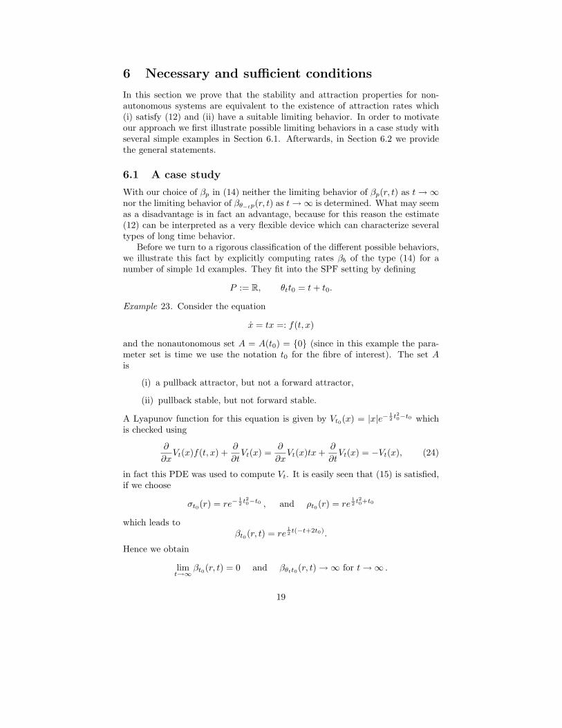
Example 23. Consider the equation

x = tx =: f(t, x)

and the nonautonomous set A = A(t0) = {0} (since in this example the para-meter set is time we use the notation t0 for the fibre of interest). The set Ais

(i) a pullback attractor, but not a forward attractor,

(ii) pullback stable, but not forward stable.

A Lyapunov function for this equation is given by Vt0(x) = |x|e−12 t20−t0 which

is checked using

∂

∂xVt(x)f(t, x) +

∂

∂tVt(x) =

∂

∂xVt(x)tx +

∂

∂tVt(x) = −Vt(x), (24)

in fact this PDE was used to compute Vt. It is easily seen that (15) is satisfied,if we choose

σt0(r) = re−12 t20−t0 , and ρt0(r) = re

12 t20+t0

which leads toβt0(r, t) = re

12 t(−t+2t0).

Hence we obtain

limt→∞

βt0(r, t) = 0 and βθtt0(r, t) → ∞ for t → ∞ .

19

The first convergence reflects the pullback attraction while the divergence re-flects the non–forward convergence and the instability.

We also use this example to show that state transformations depending onthe base space can lead to a change of the notion of stability. Consider thetransformation

Ψ(t0, x) = e−12 t20x ,

then the transformed trajectory Ψ(t + t0, ϕ(t, t0, x)) satisfies the differentialequation

d

dtΨ(t + t0, ϕ(t, t0, x)) =

d

dt

(e−

12 (t+t0)

2

ϕ(t, t0, x))

= −(t + t0)e− 1

2 (t+t0)2

ϕ(t, t0, x) + e12 (t+t0)

2

(t + t0)ϕ(t, t0, x) = 0 .

And the differential equation x = 0 clearly does not have attractive sets.

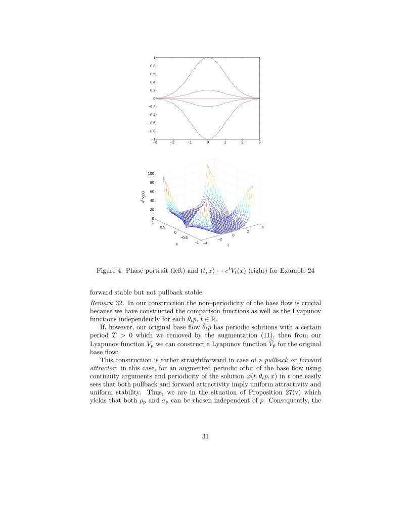
Example 24. Consider the equation

x = −tx

and the nonautonomous set A = A(t0) = {0}. The set A is

(i) not a pullback attractor, but a forward attractor,

(ii) not pullback stable, but forward stable.

Here a Lyapunov function is given by Vt0(x) = |x|e12 t20−t0 , which again can be

checked and was obtained using (24). It follows that (15) is satisfied, if wechoose

σt0(r) = re12 t20−t0 , and ρt0(r) = re−

12 t20+t0

which leads toβt0(r, t) = re

12 t(t−2t0).

Hence we obtain

βt0(r, t) → ∞ for t → ∞ and t0 fixed

βθtt0(r, t) → 0 for t → ∞

βθtt0(r, t) ≤ remax{0,−t0}2

for t ≥ 0

In this example the divergence reflects the non–pullback attraction while theconvergence shows the forward convergence and the boundedness indicates sta-bility.

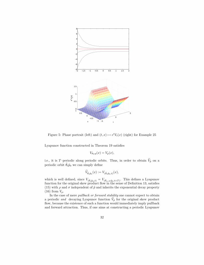
Example 25. Consider the equation

x =

{tx, t < 00, t ≥ 0

and the nonautonomous set A = A(t0) = {0}. In this case the set A is

20

(i) a pullback attractor, but not a forward attractor,

(ii) pullback and forward stable.

A Lyapunov function is obtained by appropriately modifying the V from Ex-ample 23 for t ≥ 0 which leads to

Vt0(x) =

{|x|e−

12 t20−t0 , t0 < 0

|x|e−t0 , t0 ≥ 0

which again can be checked by (24). In this example we obtain

σt0(r) =

{re−

12 t20−t0 , t0 < 0

re−t0 , t0 ≥ 0, and ρt0(r) =

{re

12 t20+t0 , t0 < 0

ret0 , t0 ≥ 0

which leads to

βt0(r, t) =

re12 t(−t+2t0), t0 < 0

r, t0 ≥ 0 and t0 − t ≥ 0β0(r, t − t0), else

.

Thus

βt0(r, t) → 0 for t → ∞ and t0 fixed

βθtt0(r, t) 6→ 0 for t → ∞

βθtt0(r, t) ≤ β0(r,max{t0, 0}) for t ≥ 0

.

The first convergence again reflects the pullback attraction while the non conver-gence to 0 indicates the non–forward convergence. However, the boundednessof β indicates the stability of A.

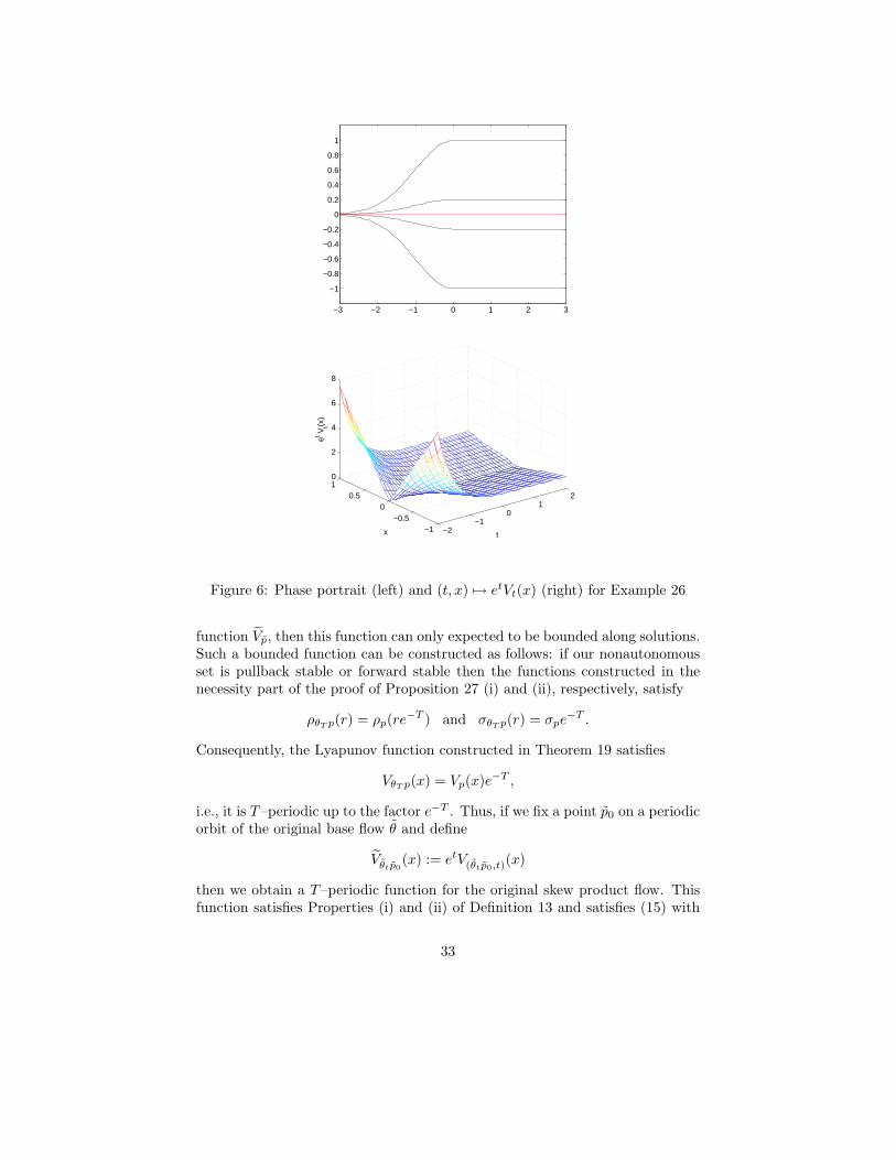
Example 26. Consider the equation

x =

{−tx, t < 00, t ≥ 0

and the nonautonomous set A = A(t0) = {0}. In this case the set A is

(i) neither a pullback attractor nor a forward attractor,

(ii) not pullback stable, but forward stable.

We obtain a Lyapunov function by appropriately modifying the V fromExample 24 for t ≥ 0 which leads to

Vt0(x) =

{|x|e

12 t20−t0 , t0 < 0

|x|e−t0 , t0 ≥ 0

which again can be checked using (24). This yields

σt0(r) =

{re

12 t20−t0 , t0 < 0

re−t0 , t0 ≥ 0and ρt0(r) =

{re−

12 t20+t0 , t0 < 0

ret0 , t0 ≥ 0

21

which leads to

βt0(r, t) =

re12 t(t−2t0), t0 < 0

r, t0 ≥ 0 and t0 − t ≥ 0β0(r, t − t0), else

.

Thus

βt0(r, t) → ∞ for t → ∞ and t0 fixed ,

βθtt0(r, t) 6→ 0 for t → ∞ ,

βθtt0(r, t) ≤ β0(r,max{t0, 0}) for t ≥ 0 .

Neither of the limits is 0 which shows that neither pullback nor forward attrac-tion holds. However, the boundedness of β indicates that A is stable.

6.2 Necessary and sufficient KL conditions

The following proposition gives necessary and sufficient conditions for our diffe-rent types of stability and attraction in terms of nonautonomous KL functions.

Proposition 27 (Necessary and Sufficient KL Conditions for Stability andAttraction). Let ϕ be an SPF in R

d and A be a nonautonomous compact setwhich is invariant under ϕ. Then

(i) A is pullback stable if and only if there exists a nonautonomous KL func-tion βp satisfying (12) locally with

limr→0

supt≥0

βp(r, t) = 0 ∀p ∈ P

on a nonautonomous set C such that for each p ∈ P there exists η(p) > 0with Bη(p)(A(θ−tp)) ⊂ C(θ−tp) for all t ≥ 0. A is globally pullback stable,if and only if in addition

supt≥0

βp(r, t) < ∞

holds for each r ≥ 0 and (12) is satisfied globally.

(ii) A is forward stable if and only if there exists a nonautonomous KL functionβp satisfying (12) locally with

limr→0

supt≥0

βθtp(r, t) = 0.

(iii) A is pullback attracting if and only if there exists a nonautonomous KLfunction βp satisfying (12) globally such that for each r > 0

limt→∞

βp(r, t) = 0, ∀p ∈ P.

22

(iv) A is forward attracting and forward stable if and only if there exists anonautonomous KL function βp satisfying (12) such that for each r > 0,p ∈ P ,

limt→∞

βθtp(r, t) = 0, ∀p ∈ P.

(v) A is uniformly attracting and pullback stable with δε independent of p, ifand only if there exists an autonomous KL function β such that (12) issatisfied with βp ≡ β.

In all these cases the nonautonomous KL–functions with the stated propertiescan be chosen such that equality holds in (14).

Proof. Sufficiency: We first show that the existence of the nonautonomousKL functions with the stated properties is sufficient for the respective stabilityproperties.

(i) Let ε > 0. Then for each p ∈ P there exists a δε(p) > 0 such that

βp(r, t) ≤ ε for all t ≥ 0 and r ≤ δε(p) .

Without loss of generality we can choose δε(p) ≤ η(p). Then, using the decayinequality (12) we get that

‖x‖A(θ−tp) ≤ δε(p) implies ‖ϕ(t, θ−tp, x)‖A(p) ≤ ε for all t ≥ 0,

proving that A is pullback stable. If the additional requirement holds then foreach r > 0, p ∈ P we find br ∈ R with

βp(r, t) ≤ br(p) for all t ≥ 0

which implies that for ε ≥ br we can choose δε(p) = r. Thus, δε(p) → ∞ asε → ∞.

(ii) Let ε > 0. Then for each p ∈ P there exists a δ = δ(p) > 0 such that

βθtp(r, t) ≤ ε for t ≥ 0 and r ≤ δ(p).

As in (i) without loss of generality we can choose δε(p) ≤ η(p). With inequality(12) we get that

‖x‖A(p) ≤ δ(p) implies ‖ϕ(t, p, x)‖A(θtp) ≤ ε for t ≥ 0. (25)

We define the nonautonomous set

C(p) :=⋃

t≥0

ϕ(t, θ−tp,Bδ(θ−tp)(A))

and show that it is contained in the ε-neighborhood of A and is forward invariantunder ϕ.

Let x ∈ C(p), then there exists a t0 ≥ 0 with x ∈ ϕ(t0, θ−t0p,Bδ(θ−t0p)(A)),

i.e. x = ϕ(t0, θ−t0p, y) for a y with ‖y‖A(θ−t0p) ≤ δ(θ−t0p). Using (25) with

x = y, t = t0 and θ−t0p instead of p we get ‖x‖A(p) ≤ ε.

23

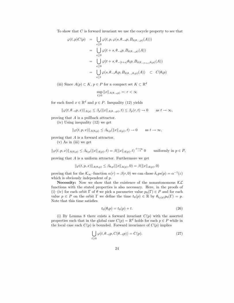
To show that C is forward invariant we use the cocycle property to see that

ϕ(t, p)C(p) =⋃

s≥0

ϕ(t, p, ϕ(s, θ−sp,Bδ(θ−sp)(A)))

=⋃

s≥0

ϕ(t + s, θ−sp,Bδ(θ−sp)(A))

=⋃

s≥0

ϕ(t + s, θ−(t+s)θtp,Bδ(θ−(t+s)θtp)(A))

=⋃

s≥t

ϕ(s, θ−sθtp,Bδ(θ−sθtp)(A)) ⊂ C(θtp)

(iii) Since A(p) ⊂ K, p ∈ P for a compact set K ⊂ Rd

supt≥0

‖x‖A(θ−tp) =: r < ∞

for each fixed x ∈ Rd and p ∈ P . Inequality (12) yields

‖ϕ(t, θ−tp, x)‖A(p) ≤ βp(‖x‖A(θ−tp), t) ≤ βp(r, t) → 0 as t → ∞,

proving that A is a pullback attractor.(iv) Using inequality (12) we get

‖ϕ(t, p, x)‖A(θtp) ≤ βθtp(‖x‖A(p), t) → 0 as t → ∞,

proving that A is a forward attractor.(v) As in (iii) we get

‖ϕ(t, p, x)‖A(θtp) ≤ βθtp(‖x‖A(p), t) = β(‖x‖A(p), t)t→∞→ 0 uniformly in p ∈ P,

proving that A is a uniform attractor. Furthermore we get

‖ϕ(t, p, x)‖A(θtp) ≤ βθtp(‖x‖A(p), 0) = β(‖x‖A(p), 0)

proving that for the K∞–function α(r) = β(r, 0) we can chose δeps(p) = α−1(ε)which is obviously independent of p.

Necessity: Now we show that the existence of the nonautonomous KLfunctions with the stated properties is also necessary. Here, in the proofs of(i)–(iv) for each orbit Γ of θ we pick a parameter value p0(Γ) ∈ P and for eachvalue p ∈ P on the orbit Γ we define the time t0(p) ∈ R by θt0(p)p0(Γ) = p.Note that this time satisfies

t0(θtp) = t0(p) + t. (26)

(i) By Lemma 8 there exists a forward invariant C(p) with the assertedproperties such that in the global case C(p) = R

d holds for each p ∈ P while inthe local case each C(p) is bounded. Forward invariance of C(p) implies

⋃

t≥0

ϕ(t, θ−tp,C(θ−tp)) = C(p). (27)

24

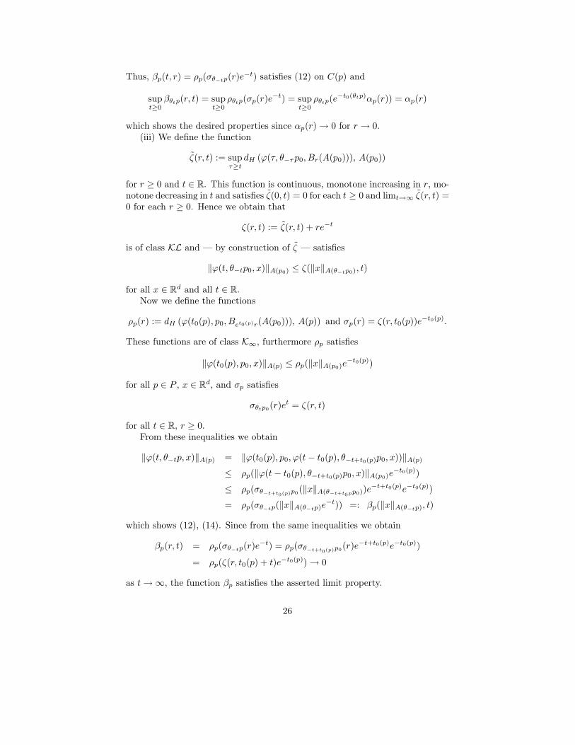
We now define functions αp by

αp(r) := dH

⋃

t≥0

ϕ(t, θ−tp,C(θ−tp) ∩ Br(A(θ−tp))), A(p)

.

From the stability property we obtain that r ≤ δε(p) implies αp(r) ≤ ε whichin particular implies αp(r) → 0 as r → 0. In the global case this also ensuresfiniteness of αp while in the non–global case (27) and the boundedness of theC(p) does so. Thus we can find class K∞ functions αp with αp ≤ αp.

Now we define

ρp(r) := αp(et0(p)r) and σp(r) := e−t0(p)r.

From the construction it immediately follows that ρp and σp are of class K∞.This definition of σp implies the inequality

σθ−tp(r)e−t = e−t0(θ−tp)re−t = e−t0(p)+te−tr = e−t0(p)r.

For x ∈ C(θ−tp) this yields

‖ϕ(t, θ−tp, x)‖A(p)

≤ αp(‖x‖A(θ−tp)) = ρp(e−t0(p)‖x‖A(θ−tp)) = ρp(σθ−tp(‖x‖A(θ−tp))e

−t).

Thus, βp(t, r) = ρp(σθ−tp(r)e−t) from (14) satisfies (12) on C(p) and

supt≥0

βp(r, t) = supt≥0

ρp(σθ−tp(r)e−t) = sup

t≥0ρp(e

−t0(p)r) = αp(r)

which shows the desired properties since αp(r) → 0 for r → 0 and αp(r) < ∞for all r ≥ 0.

(ii) We fix an arbitrary ε0 > 0 and use the nonautonomous set C(p) fromthe stability property for ε = ε0. Now we define

αp(r) := dH

⋃

t≥0

ϕ(t, p, C(p) ∩ Br(A(p))), A(θtp)

.

From the choice of C(p) we obtain that αp is bounded and from the stabilityassumption we have that αp(r) → 0 as r → 0. Thus we can find a K∞ functionαp with αp ≤ αp.

Now we proceed similar to (i), above: we define

ρp(r) := et0(p)r and σp(r) := e−t0(p)αp(r)

which yields K∞ functions satisfying

‖ϕ(t, p, x)‖A(θtp) ≤ αp(‖x‖A(p)) = et0(p)σp(‖x‖A(p)) = et0(θtp)σp(‖x‖A(p))e−t

= ρθtp(σp(‖x‖A(p))e−t).

25

Thus, βp(t, r) = ρp(σθ−tp(r)e−t) satisfies (12) on C(p) and

supt≥0

βθtp(r, t) = supt≥0

ρθtp(σp(r)e−t) = sup

t≥0ρθtp(e

−t0(θtp)αp(r)) = αp(r)

which shows the desired properties since αp(r) → 0 for r → 0.(iii) We define the function

ζ(r, t) := supτ≥t

dH (ϕ(τ, θ−τp0, Br(A(p0))), A(p0))

for r ≥ 0 and t ∈ R. This function is continuous, monotone increasing in r, mo-notone decreasing in t and satisfies ζ(0, t) = 0 for each t ≥ 0 and limt→∞ ζ(r, t) =0 for each r ≥ 0. Hence we obtain that

ζ(r, t) := ζ(r, t) + re−t

is of class KL and — by construction of ζ — satisfies

‖ϕ(t, θ−tp0, x)‖A(p0) ≤ ζ(‖x‖A(θ−tp0), t)

for all x ∈ Rd and all t ∈ R.

Now we define the functions

ρp(r) := dH (ϕ(t0(p), p0, Bet0(p)r(A(p0))), A(p)) and σp(r) = ζ(r, t0(p))e−t0(p).

These functions are of class K∞, furthermore ρp satisfies

‖ϕ(t0(p), p0, x)‖A(p) ≤ ρp(‖x‖A(p0)e−t0(p))

for all p ∈ P , x ∈ Rd, and σp satisfies

σθtp0(r)et = ζ(r, t)

for all t ∈ R, r ≥ 0.From these inequalities we obtain

‖ϕ(t, θ−tp, x)‖A(p) = ‖ϕ(t0(p), p0, ϕ(t − t0(p), θ−t+t0(p)p0, x))‖A(p)

≤ ρp(‖ϕ(t − t0(p), θ−t+t0(p)p0, x)‖A(p0)e−t0(p))

≤ ρp(σθ−t+t0(p)p0

(‖x‖A(θ−t+t0pp0))e−t+t0(p)e−t0(p))

= ρp(σθ−tp(‖x‖A(θ−tp)e−t)) =: βp(‖x‖A(θ−tp), t)

which shows (12), (14). Since from the same inequalities we obtain

βp(r, t) = ρp(σθ−tp(r)e−t) = ρp(σθ

−t+t0(p)p0(r)e−t+t0(p)e−t0(p))

= ρp(ζ(r, t0(p) + t)e−t0(p)) → 0

as t → ∞, the function βp satisfies the asserted limit property.

26

(iv) We define the function

ζ(r, t) := supτ≥t

dH (ϕ(τ, p0, Br(A(p0))), A(θtp0))

for r ≥ 0 and t ∈ R. This function is continuous, monotone increasing in r, mo-notone decreasing in t and satisfies ζ(0, t) = 0 for each t ≥ 0 and limt→∞ ζ(r, t) =0 for each r ≥ 0. Hence we obtain that

ζ(r, t) := ζ(r, t) + re−t

is of class KL and — by construction of ζ — satisfies

‖ϕ(t, p0, x)‖A(θtp0) ≤ ζ(‖x‖A(p0), t)

for all x ∈ Rd and all t ∈ R.

Now we define the functions

ρp(s) := ζ(t0(p), et0(p)s) and σp(r) := dH (ϕ(−t0(p), p, Br(A(p))), A(p0)) e−t0(p).

These functions are of class K∞, furthermore ρp satisfies

ρθt0(p)p0(re−t0(p)) = ζ(r, t0(p))

for all p ∈ P , r ≥ 0, and for y = ϕ(−t0(p), p, x) the function σp satisfies

‖y‖A(p0) ≤ σp(‖x‖A(p)et0(p))

for all p ∈ P , x ∈ Rd.

From these inequalities we obtain

‖ϕ(t, p, x)‖A(θtp) = ‖ϕ(t + t0(p), p0, ϕ(−t0(p), p, x)︸ ︷︷ ︸=y

)‖A(θtp)

≤ ζ(‖y‖A(p0), t + t0(p))

= ρθt0(p)+tp0(‖y‖A(p0)e

−t0(p)−t)

= ρθtp(‖y‖A(p0)e−t0(p)e−t)

≤ ρθtp(σp(‖x‖A(p))e−t) =: βθtp(‖x‖A(p), t)

which shows (12), (14). Since by the same computation we obtain

βθtp(r, t) = ρθtp(σp(r)e−t) = ρθt0(p)+tp0

(σp(r)et0(p)e−t0(p)−t)

= ζ(σp(r)et0(p), t0(p) + t) → 0

as t → ∞, the function βp satisfies the asserted limit property.(v) From the uniformity of the attraction we obtain that for all ε > 0 and

all R ≥ 0 there exists T > 0 such that for all p ∈ P the inequality ‖x‖A(p) ≤ Rimplies ‖Φ(s, p, x)‖A(θtp) ≤ ε for all t ≥ T .

27

The stability assumption yields that for each ε > 0 there exists δε > 0 suchthat for all p ∈ P the inequality ‖x‖A(θ−tp) ≤ δε implies ‖Φ(t, θ−tp, x)‖A(p) ≤ εfor all t ≥ 0. By substituting θ−tp → p this yields the implication

‖x‖A(p) ≤ δ ⇒ ‖Φ(t, p, x)‖A(θtp) ≤ ε.

Thus, [11, Remark B.1.5] or [21] imply the existence of β ∈ KL with

‖Φ(t, p, x)‖A(θtp) ≤ β(‖x‖A(p), t)

for all t ≥ 0, p ∈ P and x ∈ Rd. By Sontag’s KL–Lemma [27] each KL–function

is also a nonautonomous KL–function with σ and ρ independent of p, and theassertion follows.

Remark 28. Note that the functions ρp and σp constructed in (i)–(iv) satisfythe continuity assumptions in Theorem 21 if the respective functions αp andζ used in the construction satisfy this property. In (i) and (ii) we can use theregularization techniques from [11, Appendix B] in order to obtain this propertywhile in (iii) and (iv) this property is inherited from the continuity assumptionon (t, x) 7→ ‖ϕ(t, p, x)‖A(θtp) in Theorem 21.

In (v), again the regularization techniques from [11, Appendix B] can beapplied in order to obtain Lipschitz continuity of ρ−1 and σ.

6.3 Necessary and sufficient Lyapunov function conditions

The following main theorem of our paper combines Theorem 19 and Proposition27.

Theorem 29. For a nonautonomous system and a nonautonomous compactand invariant set A the following properties hold.

(i) A is pullback stable if and only if there exists a local Lyapunov functionsatisfying (15) and (16) with

limr→0

supt≥0

σθ−tp(r)e−t = 0.

on a nonautonomous set C(p) such that for each p ∈ P there exists η(p) >0 with Bη(p)(A(θ−tp)) ⊂ C(θ−tp) for all t ≥ 0. A is globally pullbackstable if and only if, in addition, the Lyapunov function is global and

supt≥0

σθ−tp(r)e−t < ∞

holds for each r ≥ 0.

(ii) A is forward stable if and only if there exists a local Lyapunov functionsatisfying (15) and (16) with

limr→0

supt≥0

ρθtp(re−t) = 0.

28

(iii) A is a pullback attractor if and only if there exists a global Lyapunovfunction satisfying (15) and (16) with

limt→∞

σθ−tp(r)e−t = 0

for each r ≥ 0.

(iv) A is a forward attractor if and only if there exists a global Lyapunovfunction satisfying (15) and (16) with

limt→∞

ρθtp(re−t) = 0.

for each r ≥ 0.

(iv) A is a uniform attractor and pullback stable with δε independent of p ifand only if there exists a local Lyapunov function satisfying (15) and (16)with σp and ρp which are independent of p.

Proof. The existence of the Lyapunov functions with the stated bounds fol-lows from Proposition 27 followed by applying Theorem 19, using the fact thatthe nonautonomous KL functions in Proposition 27 are of the form βp(r, t) =ρp(σθ−tp(r)e

−t).The converse implications follow from applying Theorem 19 followed by Pro-

position 27, observing that in case (v) the independence of δε of p is immediatefrom the independence of the bounds on V of p.

Remark 30. Expressed in terms of the Lyapunov function Vp, the conditionsfrom Theorem 29 imply

(i) limr→0 sup‖x‖A(θtp)≤r supt≤0 Vθtp(x)et = 0 (pullback stability)

(etVθtp does not blow up locally for t → −∞)

sup‖x‖A(θtp)≤r supt≤0 Vθtp(x)et < ∞ for each r > 0 (global pullback

stability)(etVθtp does not blow up globally for t → −∞)

(ii) sup‖x‖A(θtp)≤r inft≥0 Vθtp(x)et > 0 for each r > 0 (forward stability)

(etVθtp does not vanish for t → ∞)

(iii) limt→−∞ Vθtp(x)et = 0 for each r > 0 (pullback attractor)(etVθtp vanishes for t → −∞)

(iv) sup‖x‖A(θtp)≤r limt→∞ Vθtp(x)et = ∞ for each r > 0 (forward attractor)

(etVθtp blows up for t → ∞)

If the bounds in (15) are tight (i.e., when σp and ρp are the smallest possiblebounds in (15), which is always the case when the Lyapunov functions aregenerated by Theorem 19), then the conditions in Theorem 29 are, in turn,implied by these Lyapunov function conditions.

29

−2 −1.5 −1 −0.5 0 0.5 1 1.5 2−8

−6

−4

−2

0

2

4

6

8

−5

0

5

−1−0.5

00.5

10

0.2

0.4

0.6

0.8

1

tx

et Vt(x

)

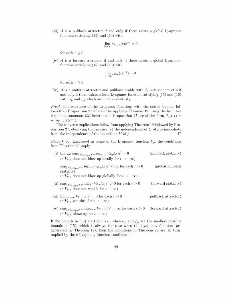
Figure 3: Phase portrait (left) and (t, x) 7→ etVt(x) (right) for Example 23

Example 31. We illustrate Theorem 29 and Remark 30 by the examples fromSection 6.1 plotting the respective phase portraits functions (t, x) 7→ etVt(x) inFigures 3.

Figure 3 shows that the Lyapunov function from example 23 vanishes bothfor t → +∞ and for t → −∞. This implies that A = {0} is a pullback attractorand pullback stable but no forward attractor and not forward stable.

Figure 4 shows that the Lyapunov function from example 24 blows up bothfor t → +∞ and for t → −∞. This implies that A = {0} is no pullback attractorand not pullback stable but it is a forward attractor and it is forward stable.

Figure 5 shows that the Lyapunov function from example 25 does neitherblow up nor vanish for t → +∞ but it vanishes for t → −∞. This implies thatA = {0} is a pullback attractor and pullback and forward stable, but is is noforward attractor.

Finally, Figure 6 shows that the Lyapunov function from example 26 doesneither blow up nor vanish for t → +∞ and blows up for t → −∞. This impliesthat A = {0} neither a pullback nor a forward attractor and that the system is

30

−3 −2 −1 0 1 2 3−1

−0.8

−0.6

−0.4

−0.2

0

0.2

0.4

0.6

0.8

1

−4−2

02

4

−1−0.5

00.5

10

20

40

60

80

100

tx

et Vt(x

)

Figure 4: Phase portrait (left) and (t, x) 7→ etVt(x) (right) for Example 24

forward stable but not pullback stable.

Remark 32. In our construction the non–periodicity of the base flow is crucialbecause we have constructed the comparison functions as well as the Lyapunovfunctions independently for each θtp, t ∈ R.

If, however, our original base flow θtp has periodic solutions with a certainperiod T > 0 which we removed by the augmentation (11), then from our

Lyapunov function Vp we can construct a Lyapunov function Vp for the originalbase flow:

This construction is rather straightforward in case of a pullback or forwardattractor: in this case, for an augmented periodic orbit of the base flow usingcontinuity arguments and periodicity of the solution ϕ(t, θtp, x) in t one easilysees that both pullback and forward attractivity imply uniform attractivity anduniform stability. Thus, we are in the situation of Proposition 27(v) whichyields that both ρp and σp can be chosen independent of p. Consequently, the

31

−2 −1.5 −1 −0.5 0 0.5 1 1.5 2−8

−6

−4

−2

0

2

4

6

8

−5

0

5

−1−0.5

00.5

10

0.5

1

1.5

tx

et Vt(x

)

Figure 5: Phase portrait (left) and (t, x) 7→ etVt(x) (right) for Example 25

Lyapunov function constructed in Theorem 19 satisfies

VθT p(x) = Vp(x),

i.e., it is T–periodic along periodic orbits. Thus, in order to obtain Vp on a

periodic orbit θtp0 we can simply define

Vθtp0(x) := V(θtp0,t)(x),

which is well defined, since V(θtp0,t) = V(θt+T p0,t+T ). This defines a Lyapunovfunction for the original skew product flow in the sense of Definition 13, satisfies(15) with ρ and σ independent of p and inherits the exponential decay property(16) from Vp.

In the case of mere pullback or forward stability one cannot expect to obtaina periodic and decaying Lyapunov function Vp for the original skew productflow, because the existence of such a function would immediately imply pullbackand forward attraction. Thus, if one aims at constructing a periodic Lyapunov

32

−3 −2 −1 0 1 2 3

−1

−0.8

−0.6

−0.4

−0.2

0

0.2

0.4

0.6

0.8

1

−2−1

01

2

−1−0.5

00.5

10

2

4

6

8

tx

et Vt(x

)

Figure 6: Phase portrait (left) and (t, x) 7→ etVt(x) (right) for Example 26

function Vp, then this function can only expected to be bounded along solutions.Such a bounded function can be constructed as follows: if our nonautonomousset is pullback stable or forward stable then the functions constructed in thenecessity part of the proof of Proposition 27 (i) and (ii), respectively, satisfy

ρθT p(r) = ρp(re−T ) and σθT p(r) = σpe

−T .

Consequently, the Lyapunov function constructed in Theorem 19 satisfies

VθT p(x) = Vp(x)e−T ,

i.e., it is T–periodic up to the factor e−T . Thus, if we fix a point p0 on a periodicorbit of the original base flow θ and define

Vθtp0(x) := etV(θtp0,t)(x)

then we obtain a T–periodic function for the original skew product flow. Thisfunction satisfies Properties (i) and (ii) of Definition 13 and satisfies (15) with

33

T–periodic bounds ρp and σp. However, it only satisfies Properties (iii) ofDefinition 13 with “≤” instead of “<” implying that it remains bounded but isnot necessarily strictly decaying along solutions (in fact, it is strictly decayingif and only if the set A is attracting).

References

[1] H. Amann. Ordinary differential equations, volume 13 of de Gruyter Studiesin Mathematics. Walter de Gruyter & Co., Berlin, 1990.

[2] L. Arnold and B. Schmalfuss. Lyapunov’s second method for random dy-namical systems. J. Differential Equations, 177(1):235–265, 2001.

[3] A. Berger and S. Siegmund. On the gap between random dynamical systemsand continuous skew products. J. Dynam. Differential Equations, 15(2-3):237–279, 2003. Special issue dedicated to Victor A. Pliss on the occasionof his 70th birthday.

[4] N. P. Bhatia and G. P. Szego. Stability theory of dynamical systems. Classicsin Mathematics. Springer-Verlag, Berlin, 2002.

[5] I. U. Bronstein and A. Y. Kopanskii. Smooth Invariant Manifolds andNormal Forms. World Scientific Publishing Co., River Edge, NJ, 1994.

[6] F. Camilli, L. Grune, and F. Wirth. A generalization of Zubov’s method toperturbed systems. SIAM J. Control Optim., 40(2):496–515 (electronic),2001.

[7] C. Conley. Isolated invariant sets and the Morse index, volume 38 of CBMSRegional Conference Series in Mathematics. American Mathematical So-ciety, Providence, R.I., 1978.

[8] C. Conley. The gradient structure of a flow. I. Ergodic Theory Dynam.Systems, 8∗(Charles Conley Memorial Issue):11–26, 9, 1988.

[9] C. Conley and R. Easton. Isolated invariant sets and isolating blocks. InAdvances in differential and integral equations (Conf. Qualitative Theory ofNonlinear Differential and Integral Equations, Univ. Wisconsin, Madison,Wis., 1968; in memoriam Rudolph E. Langer (1894–1968)), pages 97–104.Studies in Appl. Math., No. 5. Soc. Indust. Appl. Math., Philadelphia, Pa.,1969.

[10] H. Crauel. Random point attractors versus random set attractors. J.London Math. Soc. (2), 63(2):413–427, 2001.

[11] L. Grune. Asymptotic behavior of dynamical and control systems under per-turbation and discretization, volume 1783 of Lecture Notes in Mathematics.Springer-Verlag, Berlin, 2002.

34

[12] L. Grune and P. E. Kloeden. Discretization, inflation and perturbation ofattractors. In Ergodic theory, analysis, and efficient simulation of dynami-cal systems, pages 399–416. Springer, Berlin, 2001.

[13] S. F. Hafstein. A constructive converse Lyapunov theorem on exponentialstability. Discrete Contin. Dyn. Syst., 10(3):657–678, 2004.

[14] W. Hahn. Stability of motion. Translated from the German manuscriptby Arne P. Baartz. Die Grundlehren der mathematischen Wissenschaften,Band 138. Springer-Verlag New York, Inc., New York, 1967.

[15] H. K. Khalil. Nonlinear systems. Macmillan Publishing Company, NewYork, 1992.

[16] P. E. Kloeden. A Lyapunov function for pullback attractors of nonautono-mous differential equations. In Proceedings of the Conference on NonlinearDifferential Equations (Coral Gables, FL, 1999), volume 5 of Electron.J. Differ. Equ. Conf., pages 91–102 (electronic), San Marcos, TX, 2000.Southwest Texas State Univ.

[17] P. E. Kloeden and S. Siegmund. Bifurcations and continuous transitions ofattractors in autonomous and nonautonomous systems. Internat. J. Bifur.Chaos Appl. Sci. Engrg., 15(3):743–762, 2005.

[18] J. Kurzweil. On the reversibility of the first theorem of Lyapunov concer-ning the stability of motion. Czechoslovak Math. J., 5(80):382–398, 1955.

[19] J. Kurzweil and I. Vrkoc. On the converses of Ljapunov’s theorem onstability and Persidskiı’s theorem on uniform stability. Amer. Math. Soc.Transl. (2), 29:271–288, 1963.

[20] J. A. Langa, J. C. Robinson, and A. Suarez. Stability, instability, and bifur-cation phenomena in non-autonomous differential equations. Nonlinearity,15(3):887–903, 2002.

[21] Y. Lin, E. D. Sontag, and Y. Wang. A smooth converse Lyapunov theoremfor robust stability. SIAM J. Control Optim., 34(1):124–160, 1996.

[22] J. L. Massera. On Liapounoff’s conditions of stability. Ann. of Math. (2),50:705–721, 1949.

[23] J. L. Massera. Contributions to stability theory. Ann. of Math. (2), 64:182–206, 1956.

[24] T. Nadzieja. Construction of a smooth Lyapunov function for an asympto-tically stable set. Czechoslovak Math. J., 40(115)(2):195–199, 1990.

[25] G. R. Sell. Topological dynamics and ordinary differential equations. VanNostrand Reinhold Co., London, 1971.

35

[26] E. D. Sontag. Smooth stabilization implies coprime factorization. IEEETrans. Automat. Control, 34(4):435–443, 1989.

[27] E. D. Sontag. Comments on integral variants of ISS. Systems Control Lett.,34(1-2):93–100, 1998.

[28] S. Wiggins. Introduction to applied nonlinear dynamical systems and chaos,volume 2 of Texts in Applied Mathematics. Springer-Verlag, New York, NY,2nd edition, 2003.

[29] F. W. Wilson, Jr. Smoothing derivatives of functions and applications.Trans. Amer. Math. Soc., 139:413–428, 1969.

[30] F. Wirth. A converse Lyapunov theorem for linear parameter-varying andlinear switching systems. SIAM J. Control Optim., 44(1):210–239 (electro-nic), 2005.

[31] T. Yoshizawa. Stability theory by Liapunov’s second method. Publicationsof the Mathematical Society of Japan, No. 9. The Mathematical Society ofJapan, Tokyo, 1966.

[32] V. I. Zubov. Methods of A. M. Lyapunov and their application. Trans-lation prepared under the auspices of the United States Atomic EnergyCommission; edited by Leo F. Boron. P. Noordhoff Ltd, Groningen, 1964.

36