Asymptotic normalitythrough

factorial cumulants and partitions identities∗

Konstancja Bobecka†, Paweł Hitczenko‡, Fernando Lopez-Blazquez§, Grzegorz Rempała¶, Jacek Wesołowski‖

June 23, 2011

Abstract

In the paper we develop an approach to asymptotic normality through factorial cumulants. Facto-rial cumulants arise in the same manner from factorial moments, as (ordinary) cumulants from (ordinary)moments. Another tool we exploit is a new identity for ”moments” of partitions of numbers. The generallimiting result is then used to (re)derive asymptotic normality for several models including classical dis-crete distributions, occupancy problems in some generalized allocation schemes and two models relatedto negative multinomial distribution.

1 Introduction

Convergence to normal law is one of the most important phenomena of probability. As a consequence, anumber of general methods, often based on transforms of the underlying sequence have been developed astechniques for establishing such convergence. One of these methods, called the method of moments, restson the fact that the standard normal random variable is uniquely determined by its moments and that for suchrandom variable X if (Xn) is a sequence of random variables having all moments and EXk

n → EXk for

∗KB, FLB and JW were partially supported by Spanish Ministry of Education and Science Grant MTM2007-65909. Part ofwork of KB and JW was carried while they were visiting University of Seville in March/April 2009. PH was partially supportedby NSA Grant #H98230-09-1-0062. Part of work of PH was carried out while he was at the Institute of Mathematics of the PolishAcademy of Sciences and the Technical University of Warsaw in the Fall of 2010. GR and JW were partially supported by NSFGrant DMS0840695 and NIH Grant R01CA152158. Part of work of GR was carried when he was visiting Warsaw University ofTechnology in July 2009. Part of work of JW was carried out while he was visiting Medical College of Georgia in January/February2009.

†Wydział Matematyki i Nauk Informacyjnych, Politechnika Warszawska, Warszawa, Poland e-mail: bobecka@mini.pw.edu.pl‡Department of Mathematics, Drexel University, Philadelphia, USA, e-mail: phitczenko@math.drexel.edu§Facultad de Matematicas Universidad de Sevilla, Sevilla, Spain, e-mail: lopez@us.es¶Department of Biostatistics, Medical College of Georgia, Augusta, USA, e-mail: grempala@mcg.edu‖Wydział Matematyki i Nauk Informacyjnych, Politechnika Warszawska, Warszawa, Poland, e-mail: wesolo@mini.pw.edu.pl

1

all k = 1, 2, . . ., then Xnd→ X - see, e.g. [22, Theorem 2.22] or [2, Theorem 30.2]. Here and throughout

the paper we use “ d→” to denote the convergence in distribution.

Since moments are not always convenient to work with, one can often use some other characteristicsof random variables to establish the convergence to normal law. For example in one classical situation weconsider a sequence of cumulants (we recall the definition in the next section) rather than moments. On theone hand, since the kth cumulant is a continuous function of the first k moments, to prove that Xn

d→ Xinstead of convergence of moments one can use convergence of cumulants. On the other hand, all cumulantsof the standard normal distribution are zero except of the cumulant of order 2 which equals 1. This oftenmakes establishing the convergence of cumulants of (Xn) to the cumulants of the standard normal randomvariable much easier. We refer the reader to e.g. [8, Section 6.1] for more detailed discussion.

In this paper we develop an approach to asymptotic normality that is based on factorial cumulants. Theywill be discussed in the forthcoming section, here we just indicate that factorial cumulants arise in the samemanner from factorial moments, as (ordinary) cumulants from (ordinary) moments. The motivation forour work is the fact that quite often one encounters situations in which properties of random variables arenaturally expressed through factorial (rather than ordinary) moments. As we will see below, this is the case,for instance, when random variables under consideration are sums of indicator variables.

In developing our approach we first provide a simple and yet quite general sufficient condition for thecentral limit theorem in terms of factorial cumulants (see Proposition 1 in the next section). Further, as wewill see in Theorem 3 below, we show that the validity of this condition can be verified by controlling theasymptotic behavior of factorial moments. This limiting result will be then used in Section 5 to (re)deriveasymptotic normality for several models including classical discrete distributions, occupancy problems insome generalized allocation schemes (gas), and two models related to a negative multinomial distribution;they are examples of what may be called generalized inverse allocation schemes (gias). Gas was introducedin [13] and we refer the reader to chapters in books [14, 15] by the same author for more details, properties,and further references. The term “generalized inverse allocation schems” does not seem to be commonlyused in the literature; in our terminology the word “inverse” refers to inverse sampling, a sampling methodproposed in [6]. A number of distributions with “inverse” in their names reflecting the inverse sampling arediscussed in the first ([10]) and the fourth ([9]) volume on probability distributions

We believe that our approach may turn out to be useful in other situations when the factorial momentsare natural and convenient quantities to work with. We wish to mention, however, that although severalof our summation schemes are, in fact, gas or gias we do not have a general statement that would give areasonably general sufficient conditions under which a gas or a gias exhibits the asymptotic normality. It isperhaps, and interesting question, worth further investigation.

Aside from utilizing factorial cumulants, another technical tool we exploit is an identity for “moments”of partitions of natural numbers (see Proposition 2 in Section 3). As far as we know this identity is newand may be of independent interest to combinatorics community. As of now, however, we do not have anycombinatorial interpretation, neither for its validity nor for its proof.

2

2 Factorial cumulants

Let X be a random variable with the Laplace transform

φX(t) = E etX =∞∑

k=0

µktk

k!

and the cumulant transform

ψX(t) = log(φX(t)) =∞∑

k=0

κktk

k!.

Then µk = EXk and κk are, respectively, the kth moment and the kth cumulant of X , k = 0, 1, . . .. TheLaplace transform can be also expanded as

φX(t) =∞∑

k=0

νk

(et − 1

)kk!

, (2.1)

where νk is the kth factorial moment of X , that is ν0 = 1 and νk = E (X)k = EX(X − 1) . . . (X −k+1),k = 1, . . .. Here and below we use the Pochhammer symbol (x)k for the falling factorial x(x− 1) . . . (x−(k − 1)).

The sequences (µk) and (κk) satisfy µk = κk for k = 0, 1 and

κk = µk −k−1∑j=1

(k − 1j − 1

)κjµk−j , for k ≥ 2 . (2.2)

The sequences (µk) and (νk) satisfy µ0 = ν0 = 1 and

µk =k∑

j=1

S2(k, j)νj , for k ≥ 1 ,

where S2(k, j) are the Stirling numbers of the second kind defined by the identity xk =∑k

j=1 S2(k, j)(x)j

holding for any x ∈ R (see e.g. [5, (6.10) in Section 6.1]). The validity of (2.2) follows from the relation

φ(t) = exp(ψ(t)).

Following this probabilistic terminology for any sequence of real numbers (ak) one can define its cumulantsequence (bk) by ∑

aktk

k!= exp

{∑bktk

k!

}. (2.3)

This relation is known in combinatorics under the name exponential formula and its combinatorial interpre-tation when both (an) and (bn) are non–negative integers may be found, for example, in [20, Section 5.1].Properties of sequences related by (2.2) are usually proved in the combinatorial or probabilistic context,but since the proofs typically involve operating on either side of (2.2) and equating coefficients, they hold

3

universally. Thus, for example, if (an) and (bn) satisfy (2.3) then (see e.g. [20, Proposition 5.1.7] for aproof)

bk = ak −k−1∑j=1

(k − 1j − 1

)bjak−j , k ≥ 1 ,

where we adopt the usual convention that a sum over an empty range is zero. Note that the sequence b = (bk)is obtained as a transformation f = (fk) of the sequence a = (ak), that is b = f(a), where fk’s are definedrecursively by f1(x) = x1 and

fk(x) = xk −k−1∑j=1

(k − 1j − 1

)fj(x)xk−j , k > 1 . (2.4)

For a future use we record here that if b = (bn) is a cumulant sequence for a sequence of numbersa = (an), that is, b = f(a) then for any J ≥ 1

bJ =∑π⊂J

Dπ

J∏i=1

amii , where Dπ =

(−1)

JPi=1

mi−1J !

J∏i=1

(i!)mi

J∑i=1

mi

( J∑i=1

mi

m1, . . . ,mJ

), (2.5)

and where the sum is over all partitions π of a positive integer J , i.e. over all vectors π = (m1, . . . ,mJ)with nonnegative integer components which satisfy

∑Ji=1 imi = J (for a proof, see e.g. [12, Section 3.14]).

Returning for a moment to the probabilistic notions introduced at the beginning of this section we con-clude that κ = f(µ) with f defined by (2.4).

Similarly for any sequence of real numbers (ak) one can define recursively the factorial sequence (ck)by

ak =k∑

j=1

S2(k, j)cj , for k ≥ 1 .

Consequently,

bk =k∑

j=1

S2(k, j)fj(c) , k = 1, 2, . . . (2.6)

This observation is useful for proving convergence in law to the standard normal variable.

Proposition 1. Let (Sn) be a sequence of random variables having all moments. Assume that

VarSnn→∞−→ ∞ (2.7)

andESn

Var32Sn

n→∞−→ 0 . (2.8)

4

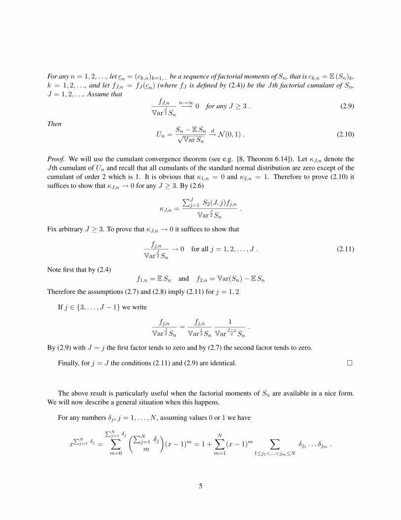
For any n = 1, 2, . . ., let cn = (ck,n)k=1,... be a sequence of factorial moments of Sn, that is ck,n = E (Sn)k,k = 1, 2, . . ., and let fJ,n = fJ(cn) (where fJ is defined by (2.4)) be the J th factorial cumulant of Sn,J = 1, 2, . . .. Assume that

fJ,n

VarJ2 Sn

n→∞−→ 0 for any J ≥ 3 . (2.9)

ThenUn =

Sn − ESn√VarSn

d→ N (0, 1) . (2.10)

Proof. We will use the cumulant convergence theorem (see e.g. [8, Theorem 6.14]). Let κJ,n denote theJ th cumulant of Un and recall that all cumulants of the standard normal distribution are zero except of thecumulant of order 2 which is 1. It is obvious that κ1,n = 0 and κ2,n = 1. Therefore to prove (2.10) itsuffices to show that κJ,n → 0 for any J ≥ 3. By (2.6)

κJ,n =

∑Jj=1 S2(J, j)fj,n

VarJ2 Sn

.

Fix arbitrary J ≥ 3. To prove that κJ,n → 0 it suffices to show that

fj,n

VarJ2 Sn

→ 0 for all j = 1, 2, . . . , J . (2.11)

Note first that by (2.4)f1,n = ESn and f2,n = Var(Sn)− ESn

Therefore the assumptions (2.7) and (2.8) imply (2.11) for j = 1, 2.

If j ∈ {3, . . . , J − 1} we write

fj,n

VarJ2 Sn

=fj,n

Varj2Sn

1

VarJ−j

2 Sn

.

By (2.9) with J = j the first factor tends to zero and by (2.7) the second factor tends to zero.

Finally, for j = J the conditions (2.11) and (2.9) are identical. �

The above result is particularly useful when the factorial moments of Sn are available in a nice form.We will now describe a general situation when this happens.

For any numbers δj , j = 1, . . . , N , assuming values 0 or 1 we have

xPN

j=1 δj =

PNj=1 δj∑m=0

(∑Nj=1 δjm

)(x− 1)m = 1 +

N∑m=1

(x− 1)m∑

1≤j1<...<jm≤N

δj1 . . . δjm .

5

Therefore if (ε1, . . . , εN ) is a random vector valued in {0, 1}N and S =∑N

i=1 εi then

E etS = 1 +∞∑

m=1

(et − 1

)m ∑1≤j1<...<jm≤N

P(εj1 = εj2 = . . . = εjm = 1) .

Comparing this formula with (2.1) we conclude that factorial moments of S have the form

E(S)k = k!∑

1≤j1<...<jk≤N

P(εj1 = εj2 = . . . = εjk= 1) =: ck , k = 1, 2, . . . . (2.12)

If, in addition, the random variables (ε1, . . . , εN ) are exchangeable then the above formula simplifies to

E(S)k = (N)k P(ε1 = . . . = εk = 1) =: ck , k = 1, 2, . . . . (2.13)

As we will see in Section 5 our sufficient condition for asymptotic normality will work well for severalsetups falling in such a scheme. This will be preceded by a derivation of new identities for integer partitionswhich will give a major enhancement of the tools we will use to prove limit theorems.

3 Partitions identities

Recall that a partition π of a positive integer J is any vector π = (m1, . . . ,mJ) with nonnegative integercomponents which satisfy

∑Ji=1 imi = J . As we discussed earlier (see (2.5)) if b = (bn) = f(a) is a

cumulant sequence of a = (an) with f defined by (2.4) then

bJ =∑π⊂J

Dπ

J∏i=1

amii ,

with (Dπ) as in (2.5). Note that for J ≥ 2 ∑π⊂J

Dπ = 0 . (3.14)

This follows from the fact that all the cumulants of the constant random variable X = 1 a.s. are zero exceptof the first one.

For π = (m1, . . . ,mJ) we denote Hπ(s) =∑J

i=1 ismi, s = 0, 1, 2 . . .. The main result of this section

is the identity which extends considerably (3.14).

Proposition 2. Assume J ≥ 2. Let I ≥ 1 and si ≥ 1, i = 1, . . . , I be such that

I∑i=1

si ≤ J + I − 2 .

Then ∑π⊂J

Dπ

I∏i=1

Hπ(si) = 0 . (3.15)

6

Proof. We use induction with respect to J . Note that if J = 2 than I may be arbitrary but si = 1 for alli = 1, . . . , I . Thus the identity (3.15) follows from (3.14) since Hπ(1) = J for any J and any π ⊂ J .

Now assume that the result holds true for J = 2, . . . ,K − 1, and consider the case of J = K. That is,we want to study ∑

π⊂K

Dπ

I∏i=1

Hπ(si)

under the condition∑I

i=1 si ≤ K + I − 2.

Let us introduce functions gi, i = 1, . . . ,K, by letting

gi(m1, . . . ,mK) = (m1, . . . , mK−1) =

(m1, . . . ,mi−1 + 1,mi − 1, . . . ,mK−1) if i 6= 1,K,(m1 − 1,m2, . . . ,mK−1) if i = 1,(m1, . . . ,mK−2,mK−1 + 1) if i = K .

Note that gi : {π ⊂ K : mi ≥ 1} → {π ⊂ (K − 1) : mi−1 ≥ 1}, i = 1, . . . ,K, are bijections. Here forconsistency we assume m0 = 1.

Observe that for any s, any π ⊂ K such that mi ≥ 1, and for π = gi(π) ⊂ (K − 1) we have

Hπ(s) = Hπ(s)− is + (i− 1)s = Hπ(s)− 1−As(i− 1) ,

where As(i− 1) =∑s−1

k=1

(sk

)(i− 1)k is a polynomial of the degree s− 1 in the variable i− 1 with constant

term equal to zero. In particular, for i = 1 we have Hπ(s) = Hπ(s)− 1. Therefore, expanding Hπ(s1) weobtain ∑

π⊂K

Dπ

I∏i=1

Hπ(si) =K∑

i=1

is1∑π⊂Kmi≥1

miDπ

I∏j=2

[Hπ(sj) + 1 +Asj (i− 1)

].

Note that if mi ≥ 1 then

1K!

imiDπ =

(−1)Mπ−1Mπ !

Mπ(m1−1)!K−1Qk=2

mk!(k!)mk

= − 1(K−1)!

∑K−1j=1 Dπmj if i = 1,

(−1)Mπ−1Mπ !

Mπ(mi−1)!(i−1)!(i!)mi−1KQ

k=2k 6=i

mk!(k!)mk

= 1(K−1)!Dπmi−1 if i = 2, . . . ,K,

where π = (m1, . . . , mK−1) = gi(π), respectively. Therefore,

1K

∑π⊂K

Dπ

I∏i=1

Hπ(si) = −K−1∑i=1

∑π⊂(K−1)

Dπmi

I∏j=2

[Hπ(sj) + 1] (3.16)

+K∑

i=2

∑π⊂(K−1)mi−1≥1

Dπmi−1is1−1

I∏j=2

[Hπ(sj) + 1 +Asj (i− 1)

].

7

The second term in the above expression can be written as

K−1∑i=1

∑π⊂(K−1)

Dπmi(i+ 1)s1−1I∏

j=2

[Hπ(sj) + 1 +Asj (i)

]. (3.17)

Note that

(i+ 1)s1−1I∏

j=2

[Hπ(sj) + 1 +Asj (i)

]=

s1−1∑r=0

(s1 − 1r

) I−1∑M=0

∑2≤u1<...<uM≤I

irM∏

h=1

(Hπ(suh) + 1)

∏2≤j≤I

j 6∈{u1,...,uM}

Asj (i) .

The term with r = 0 and M = I − 1 in the above expression is∏I

j=2 [Hπ(sj) + 1], thus this term of thesum (3.17) cancels with the first term of (3.16).

Hence, we need only to show that for any r ∈ {1, . . . , s1 − 1}, any M ∈ {0, . . . , I − 1}, and any2 ≤ u1 < . . . < uM ≤ I∑

π⊂(K−1)

Dπ

M∏h=1

(Hπ(suh) + 1)

K−1∑i=1

miir

∏2≤j≤I

j 6∈{u1,...,uM}

Asj (i) = 0. (3.18)

Observe that the expressionK−1∑i=1

miir

∏2≤j≤I

j 6∈{u1,...,uM}

Asj (i)

is a linear combination of Hπ functions with the largest value of an argument equal to∑2≤j≤I

j 6∈{u1,...,uM}

(sj − 1) + r .

Therefore the left-hand side of (3.18) is a respective linear combination of terms of the form

∑π⊂(K−1)

Dπ

W∏w=1

Hπ(tw) (3.19)

whereW∑

w=1

tw ≤M∑

j=1

suj−(M−W+1)+∑

2≤j≤Ij 6∈{u1,...,uM}

(sj−1)+s1−1 ≤I∑

i=1

si−(M−W+1)−(I−1−M)−1 .

But we assumed that∑I

i=1 si ≤ K + I − 2. Therefore

W∑w=1

tw ≤ K + I − 2− (M −W + 1)− (I − 1−M)− 1 = (K − 1) +W − 2 .

8

Now, by the inductive assumption it follows that any term of the form (3.19) is zero, thus proving (3.18). �

Note that in a similar way one can prove that (3.15) is no longer true when

I∑i=1

si = J + I − 1 .

Remark Richard Stanley [21] provided the following combinatorial description of the left hand side of(3.15): put

Fn(x) =∑

k

S2(n, k)xk,

and let (si) be a sequence of positive integers. Then the left hand side of (3.15) is a coefficient of xJ/J ! in∑P

(−1)|P|−1(|P| − 1)!∏B∈P

FσB(x),

where the sum ranges over all partitions P of a set {1, ..., I} into |P| nonempty pairwise disjoint subsets,and where for any such subset B ∈ P

σB =∑i∈B

si.

In the simplest case when I = 1 for any postive integer s1, the left-hand side of equation (3.15) is equal toJ !S2(s1, J). Since this is the number of surjective maps from an s1-element set to a J-element set, it mustbe 0 for s1 < J which is exactly what Proposition 2 asserts. It is not clear to us how easy it would be toshow that (3.15) holds for the larger values of I .

4 CLT - general setup

To illustrate and motivate how our approach is intended to work, consider a sequence (Sn) of Poissonrandom variables, where Sn ∼ Poisson(λn). As is well–known if λn →∞ then Un = Sn−E Sn√

VarSnconverges

in distribution to N (0, 1). To see how it follows from our approach, note that ESn = VarSn = λn andtherefore the assumptions (2.7) and (2.8) of Proposition 1 are trivially satisfied. Moreover the factorialmoments of Sn are ci,n = λi

n. Consequently,∏J

i=1 cmii,n = λJ

n for any partition π = (m1, . . . ,mJ) of J ∈ Nand thus

fJ,n = fJ(cn) =∑π⊂J

Dπ

J∏i=1

cmii,n = λJ

n

∑π⊂J

Dπ .

It now follows from the simplest case (3.14) of our partition identity that fJ,n = 0 as long as J ≥ 2. Hencethe assumption (2.9) of Proposition 1 is also trivially satisfied and we conclude the asymptotic normality of(Un).

The key in the above argument was, of course, a very simple form of the factorial moments ci,n of Sn

which resulted in factorization of the products of cmii,n in the expression for fJ,n. It is not unreasonable,

9

however, to expect that if the expression for moments does not depart too much from the form it took forPoisson variable, then with the full strength of Proposition 2 one might be able to prove the clt. This is theessence of condition (4.20) in the next result. This condition when combined with the extension of (3.14)given in Proposition 2, allows to refine considerably Proposition 1 towards a possible use in schemes ofsummation of indicators, as was suggested in the final part of Section 2.

Theorem 3. Let (Sn) be a sequence of random variables with factorial moments ci,n, i, n = 1, 2, . . ..Assume that (2.7) and (2.8) are satisfied and suppose that ci,n can be decomposed as

ci,n = Lin exp

∑j≥1

Q(n)j+1(i)jnj

, i, n = 1, 2, . . . , (4.20)

where (Ln) is a sequence of real numbers and Q(n)j is a polynomial of degree at most j such that

|Q(n)j (i)| ≤ (Ci)j ∀ i ∈ N (4.21)

with C > 0 a constant not depending on n or j. Assume further that for all J ≥ 3

LJn

nJ−1VarJ2 Sn

n→∞−→ 0. (4.22)

ThenUn =

Sn − E Sn√VarSn

d→ N (0, 1) as n→∞. (4.23)

Proof. Due to Proposition 1 we need only to show that (2.9) holds. The representation (4.20) implies

fJ,n =∑π⊂J

Dπ

J∏i=1

cmii,n = LJ

n

∑π⊂J

Dπezπ(J,n),

where

zπ(J, n) =∑j≥1

A(n)π (j)jnj

with A(n)π (j) =

J∑i=1

miQ(n)j+1(i).

Fix arbitrary J ≥ 3. To prove (2.9), in view of (4.22) it suffices to show that∑

π⊂J Dπezπ(J,n) is of order

n−(J−1). To do that, we expand ezπ(J,n) into power series to obtain

∑π⊂J

Dπezπ(J,n) =

∑π⊂J

DπeP

j≥11

jnj A(n)π (j) =

∑π⊂J

Dπ

∞∑s=0

1s!

∑j≥1

1jnj

A(n)π (j)

s

=∑s≥1

1s!

∑l≥s

1nl

∑j1,...,js≥1Ps

k=1 jk=l

1∏sk=1 jk

∑π⊂J

Dπ

s∏k=1

A(n)π (jk) .

10

We claim that whenever∑s

k=1 jk ≤ J − 2 then∑π⊂J

Dπ

s∏k=1

A(n)π (jk) = 0. (4.24)

To see this, note that by changing the order of summation in the expression for A(n)π (j) we can write it as

A(n)π (j) =

j+1∑k=0

α(n)k,j+1Hπ(k),

where (α(n)k,j ) are the coefficients of the polynomial Q(n)

j , that is Q(n)j (x) =

∑jk=0 α

(n)k,j x

k. Consequently,(4.24) follows from identity (3.15).

To handle the terms for which∑s

k=1 jk > J − 2 note that

|A(n)π (j)| ≤ (CJ)j+1

J∑i=1

mi < K (CJ)j ,

where K > 0 is a constant depending only on J (and not on the partition π). Hence,∣∣∣∣∣∑π⊂J

Dπ

s∏k=1

A(n)π (jk)

∣∣∣∣∣ ≤∑π⊂J

|Dπ|s∏

k=1

K (CJ)jk ≤ CKs(CJ)Ps

k=1 jk , (4.25)

where C =∑

π⊂J |Dπ| is a constant depending only on J . Therefore, restricting the sum according to(4.24) and using (4.25) we get∣∣∣∣∣∑

π⊂J

Dπezπ(J,n)

∣∣∣∣∣ ≤∑s≥1

1s!

∑l≥max{s,J−1}

1nl

∑j1,...,js≥1Ps

k=1 jk=l

1∏sk=1 jk

∣∣∣∣∣∑π⊂J

Dπ

s∏k=1

A(n)π (jk)

∣∣∣∣∣≤ C

∑s≥1

Ks

s!

∑l≥J−1

1nlls(CJ)l .

Here we used the inequality ∑j1,...,js≥1Ps

k=1 jk=l

1∏sk=1 jk

< ls ,

which may be seen by trivially bounding the sum by the number of its terms. Now we change the order ofsummations arriving at∣∣∣∣∣∑π⊂J

Dπezπ(J,n)

∣∣∣∣∣ ≤ C∑

l≥J−1

(CJ

n

)l∑s≥1

(lK)s

s!≤ C

∑l≥J−1

(CJeK

n

)l

= C

(CJeK

n

)J−1∑l≥0

(CJeK

n

)l

.

The result follows since for n sufficiently large (such that CJeK < n) the series in the last expressionconverges. �

Remark 4. A typical way Theorem 3 will be applied is as follows. Assume that ESn and VarSn are of thesame order n. Then obviously, (2.7) and (2.8) are satisfied. Assume also that (4.20) and (4.21) hold andthat Ln is also of order n. Then clearly (4.22) is satisfied and thus (4.23) holds true.

11

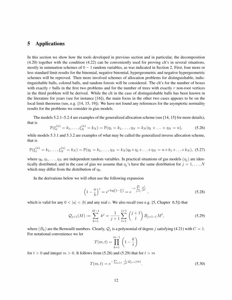
5 Applications

In this section we show how the tools developed in previous section and in particular, the decomposition(4.20) together with the condition (4.22) can be conveniently used for proving clt’s in several situations,mostly in summation schemes of 0− 1 random variables, as was indicated in Section 2. First, four more orless standard limit results for the binomial, negative binomial, hypergeometric and negative hypergeometricschemes will be reproved. Then more involved schemes of allocation problems for distinguishable, indis-tinguishable balls, colored balls, and random forests will be considered. The clt’s for the number of boxeswith exactly r balls in the first two problems and for the number of trees with exactly r non-root verticesin the third problem will be derived. While the clt in the case of distinguishable balls has been known inthe literature for years (see for instance [16]), the main focus in the other two cases appears to be on thelocal limit theorems (see, e.g. [14, 15, 19]). We have not found any references for the asymptotic normalityresults for the problems we consider in gias models.

The models 5.2.1–5.2.4 are examples of the generalized allocation scheme (see [14, 15] for more details),that is

P(ξ(n)1 = k1, . . . , ξ

(n)N = kN ) = P(η1 = k1, . . . , ηN = kN |η1 + . . .+ ηN = n), (5.26)

while models 5.3.1 and 5.3.2 are examples of what may be called the generalized inverse allocation scheme,that is

P(ξ(n)1 = k1, . . . , ξ

(n)N = kN ) = P(η1 = k1, . . . , ηN = kN |η0+η1+. . .+ηN = n+k1+. . .+kN ), (5.27)

where η0, η1, . . . , ηN are independent random variables. In practical situations of gas models (ηj) are iden-tically distributed, and in the case of gias we assume that ηj’s have the same distribution for j = 1, . . . , Nwhich may differ from the distribution of η0.

In the derivations below we will often use the following expansion

(1− a

b

)c= ec log(1−a

b ) = e−c

∞Pj=1

aj

jbj

, (5.28)

which is valid for any 0 < |a| < |b| and any real c. We also recall (see e.g. [5, Chapter 6.5]) that

Qj+1(M) :=M−1∑k=1

kj =1

j + 1

j+1∑l=1

(j + 1l

)Bj+1−lM

l, (5.29)

where (Bk) are the Bernoulli numbers. Clearly,Qj is a polynomial of degree j satisfying (4.21) withC = 1.For notational convenience we let

T (m, t) =m−1∏k=1

(1− k

t

)for t > 0 and integer m > 0. It follows from (5.28) and (5.29) that for t > m

T (m, t) = e−

Pj≥1

1

jtjQj+1(m)

. (5.30)

12

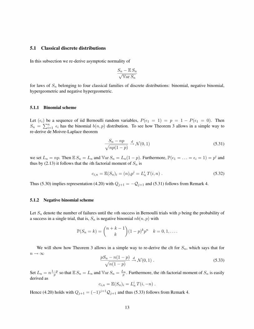
5.1 Classical discrete distributions

In this subsection we re-derive asymptotic normality of

Sn − ESn√VarSn

for laws of Sn belonging to four classical families of discrete distributions: binomial, negative binomial,hypergeometric and negative hypergeometric.

5.1.1 Binomial scheme

Let (εi) be a sequence of iid Bernoulli random variables, P (ε1 = 1) = p = 1 − P (ε1 = 0). ThenSn =

∑ni=1 εi has the binomial b(n, p) distribution. To see how Theorem 3 allows in a simple way to

re-derive de Moivre-Laplace theorem

Sn − np√np(1− p)

d→ N (0, 1) (5.31)

we set Ln = np. Then ESn = Ln and VarSn = Ln(1− p). Furthermore, P(ε1 = . . . = εi = 1) = pi andthus by (2.13) it follows that the ith factorial moment of Sn is

ci,n = E(Sn)i = (n)ipi = Li

n T (i, n) . (5.32)

Thus (5.30) implies representation (4.20) with Qj+1 = −Qj+1 and (5.31) follows from Remark 4.

5.1.2 Negative binomial scheme

Let Sn denote the number of failures until the nth success in Bernoulli trials with p being the probability ofa success in a single trial, that is, Sn is negative binomial nb(n, p) with

P(Sn = k) =(n+ k − 1

k

)(1− p)kpn k = 0, 1, . . . .

We will show how Theorem 3 allows in a simple way to re-derive the clt for Sn, which says that forn→∞

pSn − n(1− p)√n(1− p)

d→ N (0, 1) . (5.33)

Set Ln = n1−pp so that ESn = Ln and VarSn = Ln

p . Furthermore, the ith factorial moment of Sn is easilyderived as

ci,n = E(Sn)i = Lin T (i,−n) .

Hence (4.20) holds with Qj+1 = (−1)j+1Qj+1 and thus (5.33) follows from Remark 4.

13

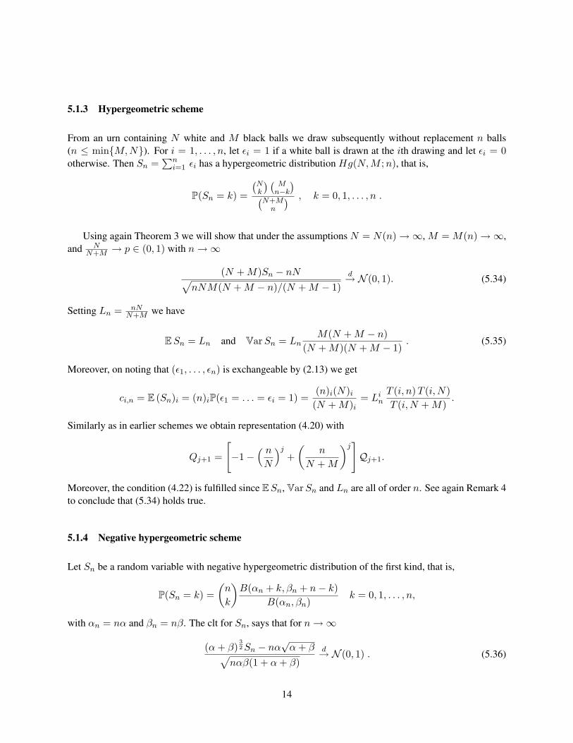
5.1.3 Hypergeometric scheme

From an urn containing N white and M black balls we draw subsequently without replacement n balls(n ≤ min{M,N}). For i = 1, . . . , n, let εi = 1 if a white ball is drawn at the ith drawing and let εi = 0otherwise. Then Sn =

∑ni=1 εi has a hypergeometric distribution Hg(N,M ;n), that is,

P(Sn = k) =

(Nk

) (M

n−k

)(N+M

n

) , k = 0, 1, . . . , n .

Using again Theorem 3 we will show that under the assumptions N = N(n) →∞, M = M(n) →∞,and N

N+M → p ∈ (0, 1) with n→∞

(N +M)Sn − nN√nNM(N +M − n)/(N +M − 1)

d→ N (0, 1). (5.34)

Setting Ln = nNN+M we have

ESn = Ln and VarSn = LnM(N +M − n)

(N +M)(N +M − 1). (5.35)

Moreover, on noting that (ε1, . . . , εn) is exchangeable by (2.13) we get

ci,n = E (Sn)i = (n)iP(ε1 = . . . = εi = 1) =(n)i(N)i

(N +M)i= Li

n

T (i, n)T (i,N)T (i,N +M)

.

Similarly as in earlier schemes we obtain representation (4.20) with

Qj+1 =

[−1−

( nN

)j+(

n

N +M

)j]Qj+1.

Moreover, the condition (4.22) is fulfilled since ESn, VarSn and Ln are all of order n. See again Remark 4to conclude that (5.34) holds true.

5.1.4 Negative hypergeometric scheme

Let Sn be a random variable with negative hypergeometric distribution of the first kind, that is,

P(Sn = k) =(n

k

)B(αn + k, βn + n− k)

B(αn, βn)k = 0, 1, . . . , n,

with αn = nα and βn = nβ. The clt for Sn, says that for n→∞

(α+ β)32Sn − nα

√α+ β√

nαβ(1 + α+ β)d→ N (0, 1) . (5.36)

14

To quickly derive it from Theorem 3 letLn = nαα+β and note that ESn = Ln and VarSn = Ln

nβ(1+α+β)(α+β)2(nα+nβ+1)

.Further, the ith factorial moment of Sn is easily derived as

ci,n = E(Sn)i = Lin

T (i, n)T (i,−αn)T (i,−(α+ β)n)

.

Thus again due to (5.30) we conclude that representation (4.20) holds with

Qj+1 =(−1− (−1)j

αj+

(−1)j

(α+ β)j

)Qj+1(i).

The final result follows by Remark 4.

5.2 Asymptotics of occupancy in generalized allocation schemes (gas)

In this subsection we will derive asymptotics for S(r)n =

∑Ni=1 I(ξ

(n)i = r) in several generalized allocation

schemes as defined at the beginning of Section 5. As we will see when n → ∞ and N/n → λ ∈ (0,∞]the order of ES(r)

n is nr/N r−1 for any r = 0, 1, . . ., and the order of VarS(r)n is the same for r ≥ 2. When

λ = ∞ and r = 0 or 1 the order of VarS(r)n is n2/N . Consequently, we will derive asymptotic normality of

Sn − ES(r)n√

nr/N r−1

when either:

(a) r ≥ 0 and λ <∞ or,

(b) r ≥ 2, λ = ∞ and nr

Nr−1 →∞,

and asymptotic normality of√NS

(r)n − ES(r)

n

n

when λ = ∞, n2

N →∞ and r = 0, 1.

Though in all the cases results read literally the same (with different asymptotic expectations and vari-ances and having different proofs) for the sake of precision we decided to repeat formulations of theoremsin each of subsequent cases.

5.2.1 Indistinguishable balls

Consider a scheme of a random distribution of n indistinguishable balls into N distinguishable boxes, suchthat all distributions are equiprobable. That is, if ξi = ξ

(n)i denotes the number of balls which fall into the

ith box, i = 1, . . . , N , then

P(ξ1 = i1, . . . , ξN = iN ) =(n+N − 1

n

)−1

15

for any ik ≥ 0, k = 1, . . . , N , such that i1 + . . .+ iN = n. Note that this is gas and that (5.26) holds withηi ∼ Geom(p), 0 < p < 1.

Let S(r)n =

∑Ni=1 I(ξi = r) denote the number of boxes with exactly r balls. Note that the distribution

of (ξ1, . . . , ξN ) is exchangeable. Moreover,

P(ξ1 = . . . = ξi = r) =

(n−ri+N−i−1

n−ri

)(n+N−1

n

) .

Therefore by (2.13) we get

ci,n = E(S(r)n )i =

(N)i(N − 1)i(n)ir

(n+N − 1)i(r+1). (5.37)

Consequently,

ES(r)n = c1,n =

N(N − 1)(n)r

(n+N − 1)r+1

and since VarS(r)n = c2,n − c21,n + c1,n we have

VarS(r)n =

N(N − 1)2(N − 2)(n)2r

(n+N − 1)2r+2−(N(N − 1)(n)r

(n+N − 1)r+1

)2

+N(N − 1)(n)r

(n+N − 1)r+1.

In the asymptotics below we consider the situation when n → ∞ and Nn → λ ∈ (0,∞]. Then for any

integer r ≥ 0N r−1

nrES(r)

n →(

λ

1 + λ

)r+1

(= 1 for λ = ∞) . (5.38)

It is also elementary but more laborious to prove that for any r ≥ 2 and λ ∈ (0,∞] or r = 0, 1 andλ ∈ (0,∞)

N r−1

nrVarS(r)

n →(

λ

1 + λ

)r+1(

1−λ(1 + λ+ (λr − 1)2

)(1 + λ)r+2

)=: σ2

r (= 1 for λ = ∞) . (5.39)

Additionally, for λ = ∞

N

n2VarS(0)

n → 1 =: σ20 and

N

n2VarS(1)

n → 4 =: σ21.

Similarly, in this case

N

n2Cov(S(0)

n , S(1)n ) → −2 and

N

n2Cov(S(0)

n , S(2)n ) → 1.

and thus for the correlation coefficient we have

ρ(S(0)n , S(1)

n ) → −1 and ρ(S(0)n , S(2)

n ) → 1. (5.40)

Now we are ready to deal with clt’s.

16

Theorem 5. Let N/n→ λ ∈ (0,∞]. Let either(a) r ≥ 0 and λ <∞or(b) r ≥ 2, λ = ∞ and nr

Nr−1 →∞.

ThenS

(r)n − ES(r)

n√nr/N r−1

d→ N (0, σ2r ) .

Proof. Note that (5.37) can be rewritten as

ci,n = Lin

T (i,N)T (i,N − 1)T (ir, n)T (i(r + 1), n+N − 1)

with Ln =N(N − 1)nr

(n+N − 1)r+1.

Therefore, similarly as in the previous cases, using (5.30) we conclude that representation (4.20) holds with

Qj+1(i) = −

[( nN

)j+(

n

N − 1

)j]Qj+1(i)−Qj+1(ri) +

(n

n+N − 1

)j

Qj+1((r + 1)i).

To conclude the proof we note that ES(r)n , VarS(r)

n and Ln are of the same order nr/N r−1 and use Re-mark 6 stated below. �

Remark 6. If ES(r)n and VarS(r)

n are of the same order and diverge to ∞ then (2.7) and (2.8) hold.Moreover, if Ln and VarS(r)

n are both of order nr/N r−1 then the left hand side of (4.22) is of order

1nJ−1

(nr

N r−1

)J2

=( nN

)J2(r−1) 1

nJ2−1.

That is, when either λ ∈ (0,∞) and r = 0, 1, . . . or λ = ∞ and r = 2, 3 . . . the condition (4.22) is satisfied.

In the remaining cases we use asymptotic correlations

Theorem 7. Let N/n→∞ and n2/N →∞. Then for r = 0, 1

√NS

(r)n − ES(r)

n

n

d→ N(0, σr

2).

Proof. Due to the second equation in (5.40) it follows that

√NS

(0)n − ES(0)

n

σ0n−√NS

(2)n − ES(2)

n

σ2n

L2

→ 0.

Therefore the result for r = 0 holds. Similarly, for r = 1 it suffices to observe that the first equation in(5.40) implies

√NS

(0)n − ES(0)

n

σ0n+√NS

(1)n − ES(1)

n

σ1n

L2

→ 0.

�

17

5.2.2 Distinguishable balls

Consider a scheme of a random distribution of n distinguishable balls into N distinguishable boxes, suchthat any such distribution is equally likely. Then, if ξi = ξ

(n)i denotes the number of balls which fall into the

ith box, i = 1, . . . , N ,

P(ξ1 = i1, . . . , ξN = iN ) =n!

i1! . . . iN !N−n

for any il ≥ 0, l = 1, . . . , N , such that i1 + . . . + iN = n. This is a gas with ηi ∼ Poisson(λ), λ > 0, in(5.26).

For a fixed nonnegative integer r let

S(r)n =

N∑i=1

I(ξi = r)

be the number of boxes with exactly r balls. Obviously, the distribution of (ξ1, . . . , ξN ) is exchangeable and

P(ξ1 = . . . = ξi = r) =n!

(r!)i(n− ir)!N−ir

(1− i

N

)n−ir

.

Therefore by (2.13) we get

ci,n = E (S(r)n )i =

(N)i(n)ir

(r!)iN ri

(1− i

N

)n−ir

. (5.41)

Consequently, for any r = 0, 1, . . .

ES(r)n = c1,n =

(n)r

(1− 1

N

)n−r

r!N r−1

and

VarS(r)n = c2,n − c21,n + c1,n =

(N − 1)(n)2r

(1− 2

N

)n−2r

(r!)2N2r−1−

(n)2r(1− 1

N

)2(n−r)

(r!)2N2(r−1)+

(n)r

(1− 1

N

)n−r

r!N r−1.

In the asymptotics below we consider the situation when n → ∞ and Nn → λ ∈ (0,∞]. Then for any

integer r ≥ 0

limn→∞

N r−1

nrES(r)

n =1r!e−

1λ

(=

1r!

for λ = ∞). (5.42)

It is also elementary but more laborious to check that for any fixed r ≥ 2 and λ ∈ (0,∞] or r = 0, 1 andλ ∈ (0,∞)

limn→∞

N r−1

nrVarS(r)

n =e−

1λ

r!

(1− e−

1λ (λ+ (λr − 1)2)

r!λr+1

):= σ2

r

(=

1r!

for λ = ∞). (5.43)

Additionally, for λ = ∞

N

n2VarS(0)

n → 12

=: σ20 and

N

n2VarS(1)

n → 2 =: σ21.

18

Similarly one can prove thatN

n2Cov(S(0)

n , S(1)n ) → −1.

Therefore for the correlation coefficients we have

ρ(S(0)n , S(1)

n ) → −1. (5.44)

SinceN

n2VarS(2)

n → 12

= σ(2)2 and

N

n2Cov(S(0)

n , S(2)n ) → 1

2we also have

ρ(S(0)n , S(2)

n ) → 1. (5.45)

We consider the cases when r ≥ 2 and λ = ∞ or r ≥ 0 and λ ∈ (0,∞).

Theorem 8. Let N/n→ λ ∈ (0,∞]. Let either(a) r ≥ 0 and λ <∞or(b) r ≥ 2, λ = ∞ and nr

Nr−1 →∞.

ThenS

(r)n − ES(r)

n√nr/N r−1

d→ N(0, σ2

r

).

Proof. Write ci,n as

ci,n = Lin e

i nN

(1− i

N

)n−ir

T (i,N)T (ir, n), where Ln =nre−

nN

r!N r−1.

Then, the representation (4.20) holds with

Qj+1(i) =(r − j

j + 1n

N

)( nN

)jij+1 −

( nN

)jQj+1(i)−Qj+1(ri).

Since ES(r)n , VarS(r)

n and Ln are of order nr/N r−1 the final result follows by Remark 6. �

Similarly as in the case of indistinguishable balls, using (5.45) and (5.44) we get

Theorem 9. Let N/n→∞ and n2/N →∞. Then for r = 0, 1

√NS

(r)n − ES(r)

n

n

d→ N(0, σr

2).

19

5.2.3 Colored balls

An urn contains NM balls, M balls of each of N colors. From the urn a simple random sample of nelements is drawn. We want to study the asymptotics of the number of colors with exactly r balls in thesample. More precisely, let ξi = ξ

(n)i denote the number of balls of color i, i = 1, . . . , N . Then

P(ξ1 = k1, . . . , ξN = kN ) =

∏Ni=1

(Mki

)(NM

n

)for all integers ki ≥ 0, i = 1, . . . , N , such that

∑Ni=1 ki = n. Obviously, the random vector (ξ1, . . . , ξN ) is

exchangeable and the gas equation (5.26) holds with ηi ∼ b(M,p), 0 < p < 1.

For an integer r ≥ 0 we want to study the asymptotics of

S(r)n =

N∑i=1

I(ξi = r).

For the ithe factorial moments we get

ci,n = (N)i P(ξ1 = . . . ξi = r) = (N)i

(Mr

)i((N−i)Mn−ri

)(NM

n

) . (5.46)

Consequently, for any r = 0, 1, . . .

ES(r)n = c1,n = N

(Mr

)((N−1)M

n−r

)(NM

n

)and

VarS(r)n = c2,n − c21,n + c1,n = N(N − 1)

(Mr

)2((N−2)Mn−2r

)(NM

n

) −N2

(Mr

)2((N−1)Mn−r

)2(NM

n

)2 +N

(Mr

)((N−1)M

n−r

)(NM

n

) .

In the asymptotics below we consider the situation when n→∞, Nn → λ ∈ (0,∞], and M = M(n) ≥ n.

Although the computational details are different, asymptotic formulas for ES(r)n , VarS(r)

n , Cov(S(0)n , S

(1)n )

and Cov(S(0)n , S

(2)n ) are literally the same as for their counterparts in the case of occupancy for distinguish-

able balls studied in Subsection 5.2.2.

First we will consider the limit result in the case r ≥ 2, λ = ∞, and r ≥ 0, λ ∈ (0,∞).

Theorem 10. Let N/n→ λ ∈ (0,∞] and M = M(n) ≥ n. Let either(a) r ≥ 0 and λ <∞or(b) r ≥ 2, λ = ∞ and nr

Nr−1 →∞.

ThenS

(r)n − ES(r)

n√nr/N r−1

d→ N(0, σ2

r

).

20

Proof. Rewrite the formula (5.46) as

ci,n = Lin

T ((M − r)i,NM − n)T (i,N)T (ri, n)T (Mi,NM)

with Ln = Nnr

(M

r

)(1− n

NM

)M(NM − n)r

.

Thus the representation (4.20) holds with

Qj+1(i) =( n

NM

)jQj+1(Mi)−

(n

NM − n

)j

Qj+1((M − r)i)−( nN

)jQj+1(i)−Qj+1(ri).

We need to see that the polynomials Qj satisfy bound (4.21). This is clearly true for each of the last twoterms in the above expression for Qj+1. For the first two terms we have∣∣∣∣∣( n

NM

)jQj+1(Mi)−

(n

NM − n

)j

Qj+1((M − r)i)

∣∣∣∣∣=

∣∣∣∣∣∣( n

NM

)jMi−1∑k=1

kj −(

n

NM − n

)j (M−r)i−1∑k=1

kj

∣∣∣∣∣∣≤

∣∣∣∣∣( n

NM

)j−(

n

NM − n

)j∣∣∣∣∣Qj+1(Mi) +

(n

NM − n

)j Mi−1∑k=(M−r)i

kj .

Since ∣∣∣∣∣( n

NM

)j−(

n

NM − n

)j∣∣∣∣∣ ≤

(n

NM − n

)j jn

NM≤(

2nNM − n

)j n

NM,

andMi−1∑

k=(M−r)i

kj ≤ rM jij+1,

and Qj+1(Mi) ≤M j+1 ij+1 we conclude that Qj’s do satisfy (4.21).

Clearly, ES(r)n , VarS(r)

n and Ln are of order nr/N r−1 and again we conclude the proof by referring toRemark 6. �

Asymptotic normality for S(1)n and S(0)

n for λ = ∞ also holds with the exact statement identical toTheorem 9 for distinguishable balls.

5.2.4 Rooted trees in random forests

Let T (N,n) denote a forest with N roots (that is N rooted trees) and n non-root vertices. Consider auniform distribution on the set of such T (N,n) forests. Let ξi = ξ

(n)i , i = 1, . . . , N , denote the number

21

of non-root vertices in the ith tree. Then (see for instance [3], [18] or [19]) for any ki ≥ 0 such that∑Ni=1 ki = n

P(ξ1 = k1, . . . , ξN = kN ) =n!∏N

i=1 ki

∏Ni=1 (ki + 1)ki−1

N(N + n)n−1.

Note that this distribution is exchangeable and that it is a gas with ηi in (5.26) given by

P(ηi = k) =λk(k + 1)k−1

k!e−(k+1)λ, k = 0, 1 . . . ; λ > 0.

We mention in passing that the distribution of ηi may be identified as Abel distribution discussed in [17]with (in their notation) p = 1 and θ = lnλ − λ. We refer to Example D in [17] for more information onAbel distributions, including further references.

For a fixed number r ≥ 0 we are interested in the number S(r)n of trees with exactly r non-root vertices

S(r)n =

N∑i=1

I(ξi = r).

Since the ith factorial moment of S(r)n is of the form

ci,n = (N)i P(ξ1 = . . . = ξi = r)

we have to find the marginal distributions of the random vector (ξ1, . . . , ξN ). From the identity

s

m∑k=0

(m

k

)(k + 1)k−1(m− k + s)m−k−1 = (s+ 1)(m+ 1 + s)m−1

which is valid for any natural m and s we easily obtain that for kj ≥ 0 such that∑i+1

j=1 kj = n

P(ξ1 = k1, . . . , ξi = ki) =n!∏i+1

j=1 kj !

(N − i)(ki+1 +N − i)ki+1−1∏i

j=1 (kj + 1)kj−1

N(N + n)n−1.

Therefore

ci,n =(r + 1)i(r−1)

(r!)i

N − i

N

(N)i(n)ri

(n+N − (r + 1)i)ri

(1− (r + 1)i

n+N

)n−1

. (5.47)

Hence

ES(r)n = c1,n =

(r + 1)r−1

r!(N − 1)(n)r

(n+N − r − 1)r

(1− r + 1

n+N

)n−1

.

Thus if N/n→ λ ∈ (0,∞] we have

N r−1

nrES(r)

n → (r + 1)r−1

r!

(λ

λ+ 1

)r

e−r+1λ+1

(=

(r + 1)r−1

r!for λ = ∞

).

Since VarS(r)n = c2,n − c21,n + c1,n elementary but cumbersome computations lead to

N r−1

nrVarS(r)

n → σ2r

22

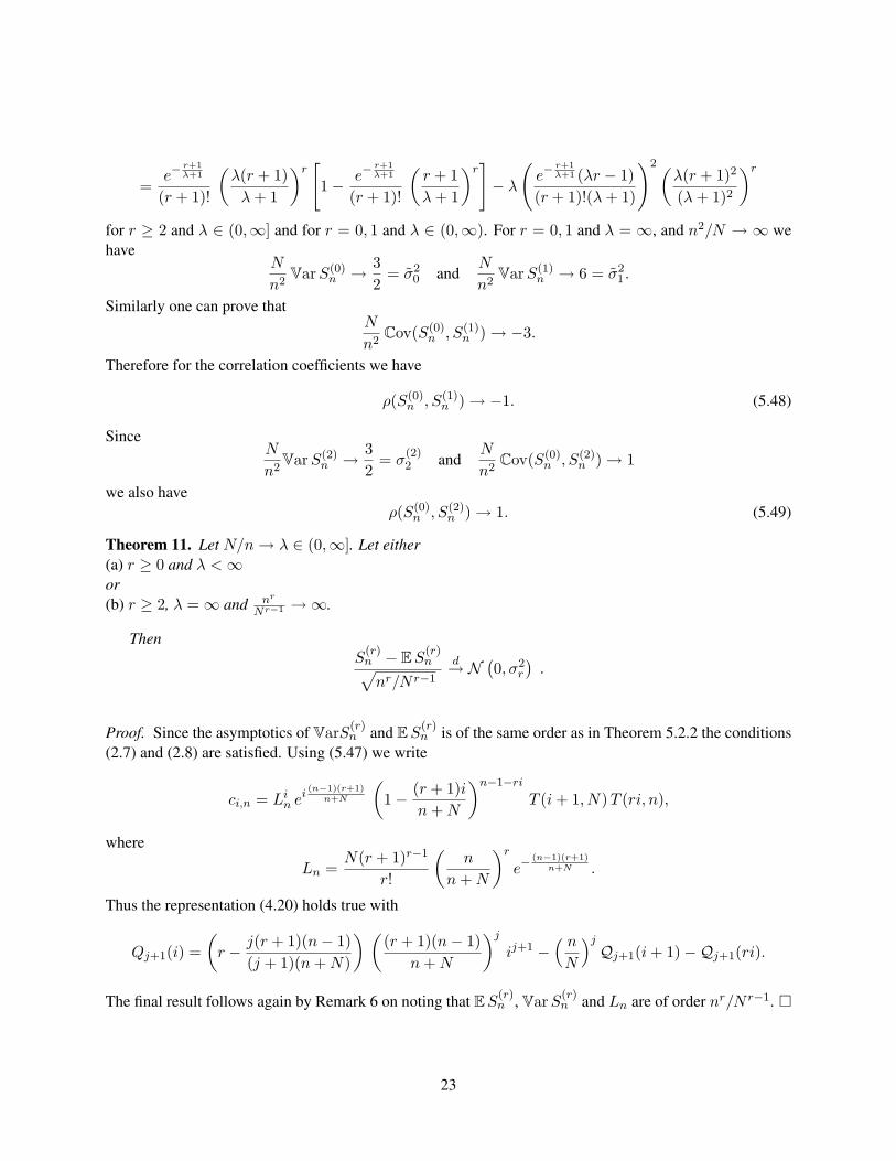
=e−

r+1λ+1

(r + 1)!

(λ(r + 1)λ+ 1

)r[1− e−

r+1λ+1

(r + 1)!

(r + 1λ+ 1

)r]− λ

(e−

r+1λ+1 (λr − 1)

(r + 1)!(λ+ 1)

)2(λ(r + 1)2

(λ+ 1)2

)r

for r ≥ 2 and λ ∈ (0,∞] and for r = 0, 1 and λ ∈ (0,∞). For r = 0, 1 and λ = ∞, and n2/N → ∞ wehave

N

n2VarS(0)

n → 32

= σ20 and

N

n2VarS(1)

n → 6 = σ21.

Similarly one can prove thatN

n2Cov(S(0)

n , S(1)n ) → −3.

Therefore for the correlation coefficients we have

ρ(S(0)n , S(1)

n ) → −1. (5.48)

SinceN

n2VarS(2)

n → 32

= σ(2)2 and

N

n2Cov(S(0)

n , S(2)n ) → 1

we also haveρ(S(0)

n , S(2)n ) → 1. (5.49)

Theorem 11. Let N/n→ λ ∈ (0,∞]. Let either(a) r ≥ 0 and λ <∞or(b) r ≥ 2, λ = ∞ and nr

Nr−1 →∞.

ThenS

(r)n − ES(r)

n√nr/N r−1

d→ N(0, σ2

r

).

Proof. Since the asymptotics of VarS(r)n and ES(r)

n is of the same order as in Theorem 5.2.2 the conditions(2.7) and (2.8) are satisfied. Using (5.47) we write

ci,n = Lin e

i(n−1)(r+1)

n+N

(1− (r + 1)i

n+N

)n−1−ri

T (i+ 1, N)T (ri, n),

where

Ln =N(r + 1)r−1

r!

(n

n+N

)r

e−(n−1)(r+1)

n+N .

Thus the representation (4.20) holds true with

Qj+1(i) =(r − j(r + 1)(n− 1)

(j + 1)(n+N)

) ((r + 1)(n− 1)

n+N

)j

ij+1 −( nN

)jQj+1(i+ 1)−Qj+1(ri).

The final result follows again by Remark 6 on noting that ES(r)n , VarS(r)

n and Ln are of order nr/N r−1. �

23

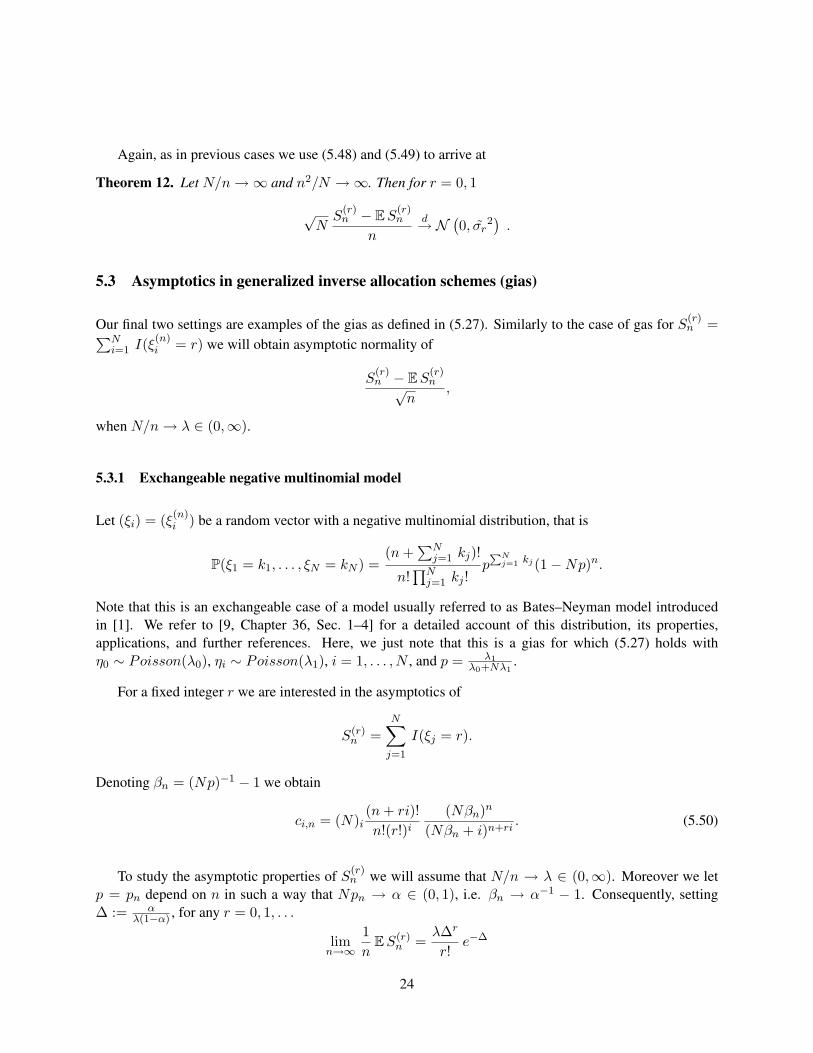
Again, as in previous cases we use (5.48) and (5.49) to arrive at

Theorem 12. Let N/n→∞ and n2/N →∞. Then for r = 0, 1

√NS

(r)n − ES(r)

n

n

d→ N(0, σr

2).

5.3 Asymptotics in generalized inverse allocation schemes (gias)

Our final two settings are examples of the gias as defined in (5.27). Similarly to the case of gas for S(r)n =∑N

i=1 I(ξ(n)i = r) we will obtain asymptotic normality of

S(r)n − ES(r)

n√n

,

when N/n→ λ ∈ (0,∞).

5.3.1 Exchangeable negative multinomial model

Let (ξi) = (ξ(n)i ) be a random vector with a negative multinomial distribution, that is

P(ξ1 = k1, . . . , ξN = kN ) =(n+

∑Nj=1 kj)!

n!∏N

j=1 kj !p

PNj=1 kj (1−Np)n.

Note that this is an exchangeable case of a model usually referred to as Bates–Neyman model introducedin [1]. We refer to [9, Chapter 36, Sec. 1–4] for a detailed account of this distribution, its properties,applications, and further references. Here, we just note that this is a gias for which (5.27) holds withη0 ∼ Poisson(λ0), ηi ∼ Poisson(λ1), i = 1, . . . , N , and p = λ1

λ0+Nλ1.

For a fixed integer r we are interested in the asymptotics of

S(r)n =

N∑j=1

I(ξj = r).

Denoting βn = (Np)−1 − 1 we obtain

ci,n = (N)i(n+ ri)!n!(r!)i

(Nβn)n

(Nβn + i)n+ri. (5.50)

To study the asymptotic properties of S(r)n we will assume that N/n → λ ∈ (0,∞). Moreover we let

p = pn depend on n in such a way that Npn → α ∈ (0, 1), i.e. βn → α−1 − 1. Consequently, setting∆ := α

λ(1−α) , for any r = 0, 1, . . .

limn→∞

1n

ES(r)n =

λ∆r

r!e−∆

24

and

limn→∞

1n

VarS(r)n =

λ∆re−∆

r!

[1− ∆re−∆

r!(1− λ(r −∆)2)

]=: σ2

r . (5.51)

Theorem 13. Let N/n→ λ ∈ (0,∞) and Npn → α ∈ (0, 1). Then for any r = 0, 1, . . .

S(r)n − ES(r)

n√n

d→ N(0, σ2

r

),

with σ2r defined in (5.51).

Proof. Write (5.50) as

ci,n = Lin e

i nNβn

T (ri+ 1,−n)T (i+ 1, N)(1 + i

Nβn

)n+riwith Ln =

nre− n

Nβn

r!N r−1βrn

.

Thus the representation (4.20) holds true with

Qj+1(i) =(r − jn

(j + 1)Nβn

) (− n

Nβn

)j

ij+1 + (−1)j+1Qj+1(ri+ 1)−( nN

)jQj+1(i).

Moreover, ES(r)n , VarS(r)

n andLn are all of order n and thus the final conclusion follows from Remark 4. �

5.3.2 Dirichlet negative multinomial model

Finally we consider exchangeable version of what is known as Dirichlet model of buying behavior intro-duced in a seminal paper by Goodhardt, Ehrenberg and Chatfield [4] and subsequently studied in numerouspapers up to the present days. This distribution is also mentioned in [9] (see Chapter 36, Sec. 6 of that book).Writing, as usually, ξ(n)

i = ξi, the distribution under study has the form

P(ξ1 = k1, . . . , ξN = kN ) =

(n+

∑Ni=1 ki

)!

n!∏N

j=1 kj !

Γ(Na+ b)ΓN (a)Γ(b)

Γ(n+ b)∏N

j=1 Γ(kj + a)

Γ(Na+ b+ n+

∑Nj=1 ki

)for any ki = 0, 1, . . ., i = 1, . . . , N . Here n > 0 is an integer and a, b > 0 are parameters. This is again agias with ηi ∼ nb(a, p), i = 1, . . . , N and η0 ∼ nb(b, p), 0 < p < 1. When a and b are integers we recalla nice interpretation of (ξ1, . . . , ξN ) via the Polya urn scheme: An urn contains b black balls and a balls ineach of N non-black colors. In subsequent steps a ball is drawn at random and returned to the urn togetherwith one ball of the same color. The experiment is continued until the nth black ball is drawn. Then ξi isthe number of balls of the ith color at the end of experiment, i = 1, . . . , N . This distribution can also beviewed as multivariate negative hypergeometric law of the second kind.

From the fact that ci,n = (N)iP(ξ1 = . . . = ξi = r) we get

ci,n = (N)i(n+ ri)!n!(r!)i

Γ(ia+ b)Γi(a)Γ(b)

Γ(n+ b)Γi(r + a)Γ((r + a)i+ n+ b)

. (5.52)

25

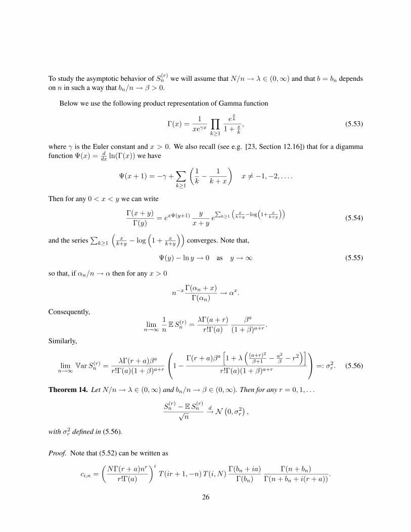
To study the asymptotic behavior of S(r)n we will assume that N/n→ λ ∈ (0,∞) and that b = bn depends

on n in such a way that bn/n→ β > 0.

Below we use the following product representation of Gamma function

Γ(x) =1

xeγx

∏k≥1

exk

1 + xk

, (5.53)

where γ is the Euler constant and x > 0. We also recall (see e.g. [23, Section 12.16]) that for a digammafunction Ψ(x) = d

dx ln(Γ(x)) we have

Ψ(x+ 1) = −γ +∑k≥1

(1k− 1k + x

)x 6= −1,−2, . . . .

Then for any 0 < x < y we can write

Γ(x+ y)Γ(y)

= exΨ(y+1) y

x+ ye

Pk≥1

“x

k+y−log

“1+ x

k+y

””(5.54)

and the series∑

k≥1

(x

k+y − log(1 + x

k+y

))converges. Note that,

Ψ(y)− ln y → 0 as y →∞ (5.55)

so that, if αn/n→ α then for any x > 0

n−x Γ(αn + x)Γ(αn)

→ αx.

Consequently,

limn→∞

1n

ES(r)n =

λΓ(a+ r)r!Γ(a)

βa

(1 + β)a+r.

Similarly,

limn→∞

VarS(r)n =

λΓ(r + a)βa

r!Γ(a)(1 + β)a+r

1−Γ(r + a)βa

[1 + λ

((a+r)2

β+1 − a2

β − r2)]

r!Γ(a)(1 + β)a+r

=: σ2r . (5.56)

Theorem 14. Let N/n→ λ ∈ (0,∞) and bn/n→ β ∈ (0,∞). Then for any r = 0, 1, . . .

S(r)n − ES(r)

n√n

d→ N(0, σ2

r

),

with σ2r defined in (5.56).

Proof. Note that (5.52) can be written as

ci,n =(NΓ(r + a)nr

r!Γ(a)

)i

T (ir + 1,−n)T (i,N)Γ(bn + ia)

Γ(bn)Γ(n+ bn)

Γ(n+ bn + i(r + a)).

26

Moreover, setting

hj(x) =∑k≥1

1(k + x)j+1

, x > 0, j ≥ 2.

we see that (5.54) can be developed into

Γ(x+ y)Γ(y)

= exΨ(y+1) e

Pj≥1

„(−x)j

jyj +(−x)j+1

j+1hj(y)

«.

Therefore, taking (x, y) = (ia, bn) and (x, y) = (i(r + a), n + bn) we decompose ci,n according to (4.20)where

Ln =NΓ(r + a)nr

r!Γ(a)eaΨ(1+bn)−(r+a)Ψ(1+n+bn)

and

Qj+1(i) =

[(n(r + a)bn + n

)j

−(na

bn

)j]

(−1)j+1ij +j(−n)j

j + 1[(r + a)j+1hj(bn + n)− aj+1hj(bn)

]ij+1

+(−1)j+1Qj+1(ir + 1)−( nN

)jQj+1(i).

On noting that αn/n → α implies that njgj(αn) < cj(α) uniformly in n we conclude that polynomialsQj satisfy condition (4.21). Moreover, (5.55) yields that Ln is of order n. Since ES(r)

n and VarS(r)n are of

order n too, the result follows by Remark 4. �

References

[1] BATES, G. E., NEYMAN, J. Contributions to the theory of accident proneness I. An optimistic modelof the correlation between light and severe accidents. Univ. California Publ. Statist. 1 (1952), 215–253.

[2] BILLINGSLEY, P. Probability and Measure. Wiley (3rd edition), New York 1995.

[3] CHUPRUNOV, A., FAZEKAS, I. An inequality for moments and its applications to the generalizedallocation scheme. Publ. Math. Debrecen, 76 (2010), 271–286.

[4] GOODHART, G.J., EHRENBERG, A.S.C., CHATFIELD, C. The Dirichlet: A comprehensive model ofbuying behavior. Journal of the Royal Statistical Society, Section A, 147 (part 5) (1984), 621-655.

[5] GRAHAM, R.L., KNUTH, D.E., PATASHNIK, O. Concrete Mathematics. Addison-Wesley PublishingCompany, Reading 1994.

[6] HALDANE, J. B. S. On a method of estimating frequencies. Biometrika 33 (1945), 222–225.

[7] HWANG, H-K., JANSON, S. Local limit theorems for finite and infinite urn models. Ann. Probab., 36(2008), 992–1022.

27

[8] JANSON, S. ŁUCZAK, T. RUCINSKI, A., Random Graphs. Wiley-Interscience Series in DiscreteMathematics and Optimization. Wiley-Interscience, New York 2000.

[9] JOHNSON, N. L., KOTZ, S., BALAKRISHNAN, N. Multivariate Discrete Distributions. Wiley Seriesin Probability and Statistics, Wiley-Interscience, New York 1997.

[10] JOHNSON, N. L., KOTZ, S., KEMP, A. W. Univariate Discrete Distributions, 2nd ed. Wiley Series inProbability and Statistics, Wiley-Interscience, New York 1992.

[11] KEENER, R. W., WU, W. B., On Dirichlet multinomial distributions. in: Random walk, sequentialanalysis and related topics, pp. 118–130. World Sci. Publ., Hackensack, NJ, 2006.

[12] KENDALL, M.G., STUART, A. The Advanced Theory of Statistics. Vol. 1: Distribution Theory.Addison-Wesley Publ. Comp., Reading 1969.

[13] KOLCHIN, V. F. A certain class of limit theorems for conditional distributions. Litovsk. Mat. Sb. 8(1968), 53–63.

[14] KOLCHIN, V. F. Random Graphs. Encyclopedia of Mathematics and its Applications, vol. 53. Cam-bridge Univ. Press, Cambridge 1999.

[15] KOLCHIN, V. F. Random Mappings. Optimization Software Inc. Publications Division, New York1986.

[16] KOLCHIN, V.F., SEVASTYANOV, B.A., CHISTYAKOV, V.P. Random Allocations. Winston & Sons,Washington 1978.

[17] LETAC, G., MORA, M. Natural real exponential families with cubic variance functions. Ann. Statist.18 (1990), 1 – 37.

[18] PAVLOV, YU. L. Limit theorems for the number of trees of a given size in a random forest. Mat.Sbornik 103 (145) (1977), 335 – 345.

[19] PAVLOV, YU. L. Random forests. VSP Utrecht 2000.

[20] STANLEY, R.P. Enumerative Combinatorics, Vol. 2. Cambridge Univ. Press, Cambridge 1999.

[21] STANLEY, R.P. Personal communication, (2009).

[22] VAN DER VAART, A.W. Asymptotic Statistics. Cambridge University Press, Cambridge 1998.

[23] WHITTAKER, E. T., WATSON, G. N., A Course of Modern Analysis (4th ed. reprinted). CambridgeUniv. Press. Cambridge 1996.

28