asymptotic enumeration in pattern avoidance and in...
TRANSCRIPT
ASYMPTOTIC ENUMERATION IN PATTERN AVOIDANCE AND IN THE THEORYOF SET PARTITIONS AND ASYMPTOTIC UNIFORMITY
By
MICAH SPENCER COLEMAN
A DISSERTATION PRESENTED TO THE GRADUATE SCHOOLOF THE UNIVERSITY OF FLORIDA IN PARTIAL FULFILLMENT
OF THE REQUIREMENTS FOR THE DEGREE OFDOCTOR OF PHILOSOPHY
UNIVERSITY OF FLORIDA
2008
1
c© 2008 Micah Spencer Coleman
2
I dedicate this dissertation with love and pride to the memory of Juliana Cole, whose
curiosity and lifelong devotion to learning have defined my family and instilled in me what
was critical to survive my graduate career. Enjoy the bagpipes, Grandmother.
3

ACKNOWLEDGMENTS
My deepest love and admiration to my wife Hiroko. While studying in a foreign
language in a foreign land, she took up two of the hardest imaginable roles, that of
military spouse and that of mathematician caretaker. Daisuki! I thank my parents Bob
and Bobbi Coleman, my brother Matt, and mi vecino Abby for their patience, humor, and
integrity. Great thanks go to Professors Julie Miller, Tina Carter, and Norm Levin, for
first introducing me to “real math”, to our Graduate Coordinator Paul Robinson, and to
the greatest advisory committee ever assembled, Professors David Drake, Meera Sitharam,
Andrew Vince, and Neil White. I am honored and humbled to be associated with each of
them. Finally, my deepest respect and appreciation are held for my advisor, Bona Miklos.
4

TABLE OF CONTENTS
page
ACKNOWLEDGMENTS . . . . . . . . . . . . . . . . . . . . . . . . . . . . . . . . . 4
LIST OF FIGURES . . . . . . . . . . . . . . . . . . . . . . . . . . . . . . . . . . . . 7
ABSTRACT . . . . . . . . . . . . . . . . . . . . . . . . . . . . . . . . . . . . . . . . 8
CHAPTER
1 INTRODUCTION . . . . . . . . . . . . . . . . . . . . . . . . . . . . . . . . . . 10
1.1 Asymptotic Enumeration . . . . . . . . . . . . . . . . . . . . . . . . . . . . 101.2 Notation for Asymptotic Growth Rates . . . . . . . . . . . . . . . . . . . . 101.3 Generating Functions . . . . . . . . . . . . . . . . . . . . . . . . . . . . . . 11
2 PATTERN AVOIDANCE IN PERMUTATIONS AVOIDING A MONOTONEPATTERN . . . . . . . . . . . . . . . . . . . . . . . . . . . . . . . . . . . . . . 12
2.1 Permutations and Permutation Patterns . . . . . . . . . . . . . . . . . . . 122.2 An Open Problem by M. Atkinson . . . . . . . . . . . . . . . . . . . . . . 242.3 Generating Trees . . . . . . . . . . . . . . . . . . . . . . . . . . . . . . . . 262.4 “Hat” Notation . . . . . . . . . . . . . . . . . . . . . . . . . . . . . . . . . 312.5 Monotone Increasing Patterns q . . . . . . . . . . . . . . . . . . . . . . . . 332.6 The Pattern q = 123 . . . . . . . . . . . . . . . . . . . . . . . . . . . . . . 38
3 PATTERN PACKING . . . . . . . . . . . . . . . . . . . . . . . . . . . . . . . . 53
3.1 General Pattern Packing . . . . . . . . . . . . . . . . . . . . . . . . . . . . 533.2 Pattern Packing in 123-avoiding Permutations . . . . . . . . . . . . . . . . 573.3 Pattern Packing in q-avoiding Permutations . . . . . . . . . . . . . . . . . 593.4 Packing Density and Further Directions . . . . . . . . . . . . . . . . . . . . 61
4 ASYMPTOTIC NORMALITY AND UNIFORMITY . . . . . . . . . . . . . . . 63
4.1 Probability Theory . . . . . . . . . . . . . . . . . . . . . . . . . . . . . . . 634.2 Triangular Arrays . . . . . . . . . . . . . . . . . . . . . . . . . . . . . . . . 644.3 Asymptotic Normality . . . . . . . . . . . . . . . . . . . . . . . . . . . . . 654.4 Asymptotic Uniformity . . . . . . . . . . . . . . . . . . . . . . . . . . . . . 664.5 Generating Polynomials with Real, Non-Positive Roots . . . . . . . . . . . 684.6 Asymptotic Normality Implies Asymptotic Uniformity . . . . . . . . . . . 71
5 ON THE ROOTS OF THE BELL POLYNOMIALS . . . . . . . . . . . . . . . . 74
5.1 Stirling Numbers of the Second Kind . . . . . . . . . . . . . . . . . . . . . 745.2 Bell Polynomials . . . . . . . . . . . . . . . . . . . . . . . . . . . . . . . . 775.3 Bounds on the Roots of the Bell Polynomials . . . . . . . . . . . . . . . . . 805.4 Asymptotics of the Roots of the Bell Polynomials . . . . . . . . . . . . . . 83
5
REFERENCES . . . . . . . . . . . . . . . . . . . . . . . . . . . . . . . . . . . . . . . 88
BIOGRAPHICAL SKETCH . . . . . . . . . . . . . . . . . . . . . . . . . . . . . . . . 91
6

LIST OF FIGURES
Figure page
2-1 The permutation 3142. . . . . . . . . . . . . . . . . . . . . . . . . . . . . . . . . 13
2-2 The permutation 532614. . . . . . . . . . . . . . . . . . . . . . . . . . . . . . . . 25
2-3 The permutation 865321947. . . . . . . . . . . . . . . . . . . . . . . . . . . . . . 27
2-4 A rooted tree. . . . . . . . . . . . . . . . . . . . . . . . . . . . . . . . . . . . . . 28
2-5 The complete binary tree. . . . . . . . . . . . . . . . . . . . . . . . . . . . . . . 29
2-6 The Fibonacci tree. . . . . . . . . . . . . . . . . . . . . . . . . . . . . . . . . . . 30
2-7 T(123,132). . . . . . . . . . . . . . . . . . . . . . . . . . . . . . . . . . . . . . . 32
2-8 Tree in W(123,231) rooted at 42153 . . . . . . . . . . . . . . . . . . . . . . . . . 40
2-9 The layered permutation 213654 with layers 21, 3, and 654 . . . . . . . . . . . . 41
3-1 The permutation W (6) = 342516 . . . . . . . . . . . . . . . . . . . . . . . . . . . 55
7
Abstract of Dissertation Presented to the Graduate Schoolof the University of Florida in Partial Fulfillment of theRequirements for the Degree of Doctor of Philosophy
ASYMPTOTIC ENUMERATION IN PATTERN AVOIDANCE AND IN THE THEORYOF SET PARTITIONS AND ASYMPTOTIC UNIFORMITY
By
Micah Spencer Coleman
May 2008
Chair: Miklos BonaMajor: Mathematics
We demonstrate asymptotic properties of some popular combinatorial objects,
including a partial answer to an open problem posed by Michael Atkinson and a general
result on conditions for the coincidence of asymptotic normality and uniformity.
For a permutation π ∈ Sn written in one line notation as π = π1π2 · · · πn, we say
π contains the pattern σ ∈ Sm if there exists a subsequence πi1 · · · πim such that for all
1 ≤ j, k ≤ m it holds that πij < πik if and only if σj < σk. Denote by sn(τ, σ) the number
of n-permutations which do not contain either of the patterns σ and τ . Letting σ′ denote
the pattern (m + 1)σ, we construct classes of patterns for which the limit supremum of
sn(123 · · · r, σ)1/n agrees with the limit supremum of sn(123 · · · r, σ′)1/n for several classes
of patterns σ. We also construct classes of permutations which avoid 123 · · · r and contain
many patterns.
Many combinatorial sequences are of the form (an,k) where n ranges over the
non-negative integers N and, for each n, there exists m = m(n) such that k ranges
from 1 to m. We call such a sequence a combinatorial distribution. Many combinatorial
distributions, upon rescaling, approach in distribution the normal distribution as n grows
to infinity, a phenomenon we call asymptotic normality. A combinatorial distribution is
said to be asymptotically uniform if, for each positive integer q and each residue class
modulo q, the sum of coefficients an,k with k ≡ r (mod q) approaches 1/q as n grows to
infinity. We call this asymptotic uniformity. We prove that if the generating polynomials
8
for a combinatorial distribution have real, nonnegative zeros, asymptotic normality implies
asymptotic uniformity. We apply this result to several sequences from the literature.
Finally, we present original results on the zeros of the Bell polynomials which were
first attained in proving the asymptotic uniformity of the Stirling numbers of the second
kind Sn,k.
9

CHAPTER 1INTRODUCTION
1.1 Asymptotic Enumeration
Enumerative combinatorics involves counting discrete objects, determining the
cardinalities of sets which are indexed by one or more integers. In many cases exact
formulae are known. However, some formulae are so convoluted as to obscure their most
telling information. In either of these cases asymptotics provide powerful methods for
understanding the classes under question.
With that said, we could define asymptotic combinatorics as the study of the growth
of combinatorial sequences indexed by an integer n as n grows without bound, n → ∞.
For a survey of these techniques, the reader is reffered to the chapter by Odlyzko [26] in
the Handbook of Combinatorics.
Definition 1. We introduce some notation to be used throughout. Let [n] denote the set
1, 2, . . . , n, and [a, b] denotes the set a, a + 1, . . . , b. N denotes the natural numbers
n ≥ 0, while P denotes the positive integers n ≥ 1.
1.2 Notation for Asymptotic Growth Rates
Let f : P → P be a function with some sort of predictable behavior. What does it
mean to understand the asymptotic behavior or growth of f? If it is anything like most
functions we encounter, as n grows arbitrarily large, the growth of f probably follows some
pattern, for example a straight line or logarithmic curve. Perhaps f acts erratically on
every small interval but has a smooth overall growth which we can mimic with some other
function g which is easier to understand.
Example 1. Define the function φ(n) = n2 + (−1)n. This function is easy to write but
not so easy to graph. However, as n grows very large we see that φ(n) is very close to the
polynomial n2.
10
Such a situation motivates Big O notation. Given two functions f and g defined on
the positive integers, we write
f(n) = O(g(n))
if there exists a nonzero constant M such that |f(n)| < |Mg(n)| for all n ≥ 1.
Similarly,
f(n) = Ω(g(n))
if there exists a constant M such that |f(n)| > |Mg(n)| for all n ≥ 1.
Finally,
f(n) ∼ g(n)
if
limn→∞
f(n)
g(n)= 1
holds.
1.3 Generating Functions
A powerful area of combinatorics is Generatingfunctionology. For surveys of the field,
the reader is referred to the texts by Wilf [40], Stanley [33], [34], and Bona [8].
Definition 2. Given a sequence (an)n≥0, the associated ordinary generating function is
the power series
f(x) =∑n≥0
anxn.
Similarly, for a sequence (an,k) defined for all n ≥ 0 and 0 ≤ k ≤ m(n) for some function
m(n), the associated generating polynomial for each n is the polynomial
gn(x) =
m(n)∑
k≥0
an,kxk.
The power is in handling these power series and polynomials to reveal information
about the sequence in question. Generating polynomials will play a fundamental role in
the last two chapters.
11

CHAPTER 2PATTERN AVOIDANCE IN PERMUTATIONS AVOIDING A MONOTONE PATTERN
2.1 Permutations and Permutation Patterns
One aspect of enumerative combinatorics, one of the simple beauties that make
it such an attractive discipline, is the ease with which it can be explained to the
non-specialist or even non-mathematician / non-scientist. We seek to count the objects in
some class of size n. For example, we may estimate the number of objects in some class
which are of size n and have statistics l, k as n grows arbitrarily large. In fact, there are
some combinatorial objects which are more easily explained to a non-mathematician than
to some of our mathematical colleagues. The case in mind is the permutation. In the
field of permutation patterns, one views a permutation in one-line notation; i.e., as an
arrangement of the numbers 1 through n for some n. That is it. While we readily admire
and appreciate the wisdom and complexity of our friends the algebraists and topologists,
there is a certain frustration and loss of momentum when trying to describe the simple
properties of permutations that we are dealing with here to such an audience. There is no
consideration of cycle structure, what set is acted upon, etc. From such a rough definition
we can pose many of the fundamental questions dealt with in this field of research.
In the first three chapters of this dissertation we introduce the concept of a
permutation pattern, survey some of the major results and trends in the field of
permutation patterns, develop a foundation for the work contained herein, and pose
further questions to be explored.
Definition 3 (rough). A permutation of length n or a permutation on [n] or an
n-permutation is an arrangement of the numbers 1 through n.
Definition 4 (rigorous). An n-permutation π is an injective mapping from the set
[n] = 1, 2, . . . , n onto itself. We denote π(i) by πi and write π as the concatenation
π1π2 · · · πn, calling the numbers π1, . . . , πn the entries of π. It should be noted that by
12
convention we allow there to be one permutation on the empty set. Finally, for each n ≥ 0
we denote by Sn the set of n-permutations.
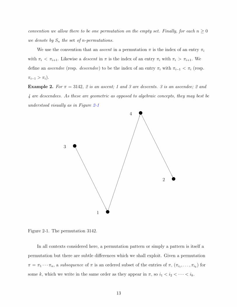
We use the convention that an ascent in a permutation π is the index of an entry πi
with πi < πi+1. Likewise a descent in π is the index of an entry πi with πi > πi+1. We
define an ascendee (resp. descendee) to be the index of an entry πi with πi−1 < πi (resp.
πi−1 > πi).
Example 2. For π = 3142, 2 is an ascent; 1 and 3 are descents. 3 is an ascendee; 2 and
4 are descendees. As these are geometric as opposed to algebraic concepts, they may best be
understood visually as in Figure 2-1
x3
x1
x4
x2
AAAAAAAAAAAAAAAAAA£
£££££££££££££££££££££££££A
AAAAAAAAAAAAAAAAA
Figure 2-1. The permutation 3142.
In all contexts considered here, a permutation pattern or simply a pattern is itself a
permutation but there are subtle differences which we shall exploit. Given a permutation
π = π1 · · · πn, a subsequence of π is an ordered subset of the entries of π, (πi1 , . . . , πik) for
some k, which we write in the same order as they appear in π, so i1 < i2 < · · · < ik.
13
Example 3. Consider the 5-permutation π = 13425. If we want to construct a subse-
quence, we have two choices of what to do with each entry πi, whether to include πi in our
subsequence or not. Therefore, we have 25 = 32 subsequences of π. We list them here in an
obvious but meaningless ordering:
Length 0 : ∅
Length 1 : 1 3 4 2 5
Length 2 : 13 14 12 15 34 32 35 42 45 25
Length 3 : 134 132 135 142 145 125 342 345 325 425
Length 4 : 1342 1345 1325 1425 3425
Length 5 : 13425
Roughly speaking, each such subsequence can be associated with some pattern, and
from this we generate vast fields of research. With such tasking, let us formalize the
concept of the permutation pattern.
Definition 5. We call a finite sequence X of distinct positive integers reduced if the
elements of the sequence form the set [n] for some n, i.e. if X is a permutation of [n].
Let X = X1X2 . . . Xn be a finite sequence of n distinct positive integers. Then,
there exists a unique permutation π ∈ Sn such that for all pairs of indices i and j with
1 ≤ i < j ≤ n,
Xi < Xj if and only if πi < πj.
So, X and π are in the same “order”, or order isomorphic. As we assumed π to be a
permutation in Sn, π is reduced, and we call π the reduction of X.
Definition 6. Let γ ∈ Sn. We say that γ contains the pattern σ ∈ Sm (m ≤ n) if there
exists a subsequence γi1γi2 · · · γim (i1 < i2 < · · · < im) whose reduction is σ. If there is no
such subsequence, we say that γ avoids the pattern σ.
14

One more note is in order on the above definition, which implicitly defines patterns.
A pattern is itself simply a permutation, but we use the two words to describe distinct
sets. We ask questions such as does the permutation π contain the pattern σ, etc. These
meanings will be clear in the context. Please also note that we will use the convention
wherever possible of letting m denote the length of a pattern σ and letting n denote the
length of a permutation π for which we want to determine σ-avoidance, etc. Much of
this dissertation will be devoted to questions surrounding the avoidance of a set of two
patterns, one of which will be monotone increasing. We will conventionally let q denote
the monotone increasing pattern in question and let r denote its length.
Example 4. The permutation 34521 contains the pattern 123, as the first three entries of
34521 are 345, which reduces to 123.
Example 5. We exhaust all patterns contained in the permutation 13425 from Example 3
by reducing all subsequences, in the same ordering as above:
Length 0 : ∅
Length 1 : 1 1 1 1 1
Length 2 : 12 12 12 12 12 21 12 21 12 12
Length 3 : 123 132 123 132 123 123 231 123 213 213
Length 4 : 1342 1234 1324 1324 2314
Length 5 : 13425
Of course, we could continue in this fashion. It is a great exercise for the beginner
in this area to exhaust the subsequences of a permutation to determine what patterns
the permutation contains or avoids and pose some conjectures. This is how one learns
anything in combinatorics, by “getting our hands dirty”, doing enough manual labor on
our combinatorial objects to get a feel for their growth and other properties.
15

Definition 7. Let σ ∈ Sm be a pattern. For each n ≥ 0 we denote by Sn(σ) the set
of all n-permutations which avoid σ, and write sn(σ) = |Sn(σ)|, i.e. the number of
n-permutations which avoid σ.
More generally, let Σ be a set of patterns. For each n ≥ 0 we denote by Sn(Σ)
the set of all n-permutations which avoid all patterns in Σ, enumerated by sn(Σ). If
Σ = σ1, σ2, . . . , σk, we write Sn(Σ) as Sn(σ1, σ2, . . . , σk) and likewise write sn(Σ) as
sn(σ1, σ2, . . . , σk), dropping the brackets.
On a historical note, the Sn and sn above may have been coined in honor of Simion
and Schmidt, whose 1985 paper [31] launched pattern avoidance and contained some
results which are still hallmarks of the field.
As the name would imply, enumerative combinatorialists most enjoy enumerating
sets, that is, determining a precise formula for the cardinality of each set which depends
only on the index or indices of that set. Unfortunately, we often find quite interesting
discrete objects whose nature is complex enough to elude precise formulae. Alas, we will
see that for most patterns σ, the sequence sn(σ) falls into the latter category. However,
all is not lost. As was briefly discussed in the introductory chapter, great information
can still be had by the asymptotics of a sequence, and many of the current results in the
field of permutation patterns involve bounds and limits which are not as strong as precise
formulae, but carry power and beauty of their own.
Let us first see some examples of patterns for which we can give an exact formula. We
will treat all patterns in Sm for 0 ≤ m ≤ 3. We will make use of the Kronecker delta δi,j,
defined by
δi,j =
1 if i = j,
0 if i 6= j.
16
Proposition 6. We have the following exact formulae for σ ∈ Sm, m = 0, 1, 2:
sn(∅) = 0,
sn(1) = δn,0,
sn(12) = 1,
sn(21) = 1.
Proof. As we can take an empty subsequence of any permutation, including the empty
permutation itself, no permutation can avoid the pattern ∅, and sn(∅) = 0.
Similarly, every non-empty permutation has a non-empty subsequence of length
1, and sn(1) = 0 unless n = 0, in which case we have s0(1) = 1, counting the sole
permutation in S0.
Note that a permutation π ∈ Sn avoiding the pattern 12 is equivalent to π having
no ascents, implying π is the unique monotone descending sequence of length n, so
sn(12) = 1. The dual statement is that avoiding the pattern 21 is equivalent to avoiding
descents, thus sn(21) = 1.
The reader may (should) have been amazed by the fact that sn(12) = sn(21) and their
dual proofs. In fact, the duality involved was that 12 and 21 are reverses of each other,
and for each n the unique permutation in Sn(12), the monotone decreasing permutation,
is the reverse of the monotone increasing permutation, the unique element of Sn(21). Of
course, one could also prove the equality with the fact that 12 and 21 are complements of
each other. Perhaps these statements also apply to longer, more interesting patterns?
17
Definition 8. Let π = π1π2 · · · πn be a permutation. We define the reverse, complement,
and algebraic inverse, resp., of π as
πR = πnπn−1 · · · π1,
πC = (n− π1 + 1)(n− π2 + 1) · · · (n− πn + 1),
π−1 = φ1φ2 · · ·φn,
where, for all 1 ≤ i ≤ n, πφi= i.
Example 7. Let π = 24315. Then, we have the eight related permutations
π = 24315,
πR = 51342,
πC = 42351,
π−1 = 41325,
πRC(= πCR) = 15324,
(πR)−1 = 25341,
(πC)−1 = 52314,
(πRC)−1 = 14352.
Of course, the algebraic inverse π−1 is just what the name would imply, the inverse
of π considered as an element of the group Sn. Such a definition as the one above may
seem crude, but we had promised to only consider these permutations as linear orders, not
group elements.
In our example of π = 24315, we made easy use of the obvious fact that R and
C commute as operators. We leave it as an exercise that they each commute with the
algebraic inverse as well.
The definition of reverse should be clear. We note that we can write each entry of πR
as πRi = πn−i+1. We can think of complement as “flipping” the permutation in a vertical
18
sense. Now that we have these definitions, we return to the question of equivalences
among patterns.
Suppose a permutation π = π1 · · · πn contains the pattern σ = σ1 · · · σm. Then, we
have a set of indices 1 ≤ p1 ≤ · · · pm ≤ n such that the reduction of the subsequence
πp1 · · · πpm is precisely σ, i.e. for all i < j,
πpi< πpj
if and only if σi < σj.
By the remarks following Definition 8, this is equivalent to the statement that, for each
pair i < j,
πRn−pi+1 > πR
n−pj+1 if and only if σRn−i+1 > σR
n−i+1.
As we run through all pairs i < j, we see that this collection of statements is equivalent to
πRpi
> πRpj
if and only if σRi > σR
j .
Altogether, π containing σ is equivalent to πR containing σR. Likewise, π containing σ
is equivalent to πC containing σC and π−1 containing σ−1. Of course, we can replace the
word “containing” by the word “avoiding” in each statement.
Critically, as the three maps ·R, ·C , and ·−1 are bijections Sn → Sn, it follows that
the number of n-permutations which avoid σ is the same as the number of n-permutations
avoiding σR, σC , σ−1. We have achieved the following result.
Lemma 1. Let σ be a pattern. Then, for all n ≥ 0,
sn(σ) = sn(σR) = sn(σC) = sn(σ−1).
In fact, we can say that each σ ∈ Sm belongs to an equivalence class of m-patterns
whose sequences sn are equal.
Definition 9. We say the patterns σ and τ are Wilf-equivalent if sn(σ) = sn(τ) holds for
all n ≥ 0. This leads naturally to the definition of the Wilf-equivalence class of a pattern σ
as the set of all patterns which are Wilf-equivalent to σ.
19
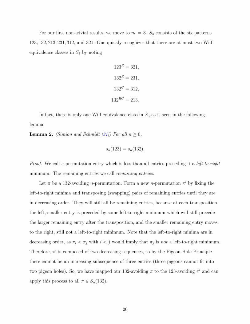
For our first non-trivial results, we move to m = 3. S3 consists of the six patterns
123, 132, 213, 231, 312, and 321. One quickly recognizes that there are at most two Wilf
equivalence classes in S3 by noting
123R = 321,
132R = 231,
132C = 312,
132RC = 213.
In fact, there is only one Wilf equivalence class in S3 as is seen in the following
lemma.
Lemma 2. (Simion and Schmidt [31]) For all n ≥ 0,
sn(123) = sn(132).
Proof. We call a permutation entry which is less than all entries preceding it a left-to-right
minimum. The remaining entries we call remaining entries.
Let π be a 132-avoiding n-permutation. Form a new n-permutation π′ by fixing the
left-to-right minima and transposing (swapping) pairs of remaining entries until they are
in decreasing order. They will still all be remaining entries, because at each transposition
the left, smaller entry is preceded by some left-to-right minimum which will still precede
the larger remaining entry after the transposition, and the smaller remaining entry moves
to the right, still not a left-to-right minimum. Note that the left-to-right minima are in
decreasing order, as πi < πj with i < j would imply that πj is not a left-to-right minimum.
Therefore, π′ is composed of two decreasing sequences, so by the Pigeon-Hole Principle
there cannot be an increasing subsequence of three entries (three pigeons cannot fit into
two pigeon holes). So, we have mapped our 132-avoiding π to the 123-avoiding π′ and can
apply this process to all π ∈ Sn(132).
20

To see that this process is reversible, we fix the left-to-right minima of π′, leaving
blanks at the other indices and placing the remaining entries in a sack. Moving left to
right, we fill each blank with the least entry still in our sack which is larger than the
rightmost left-to-right minimum to the left of said blank. Now we have a permutation π,
which we claim to be 132-avoiding. Indeed, if there were a copy of 132, then there would
be a copy of 132 beginning with a left-to-right minimum, however this is a contradiction as
the entries following and larger than each left-to-right minimum are increasing. Thus, we
have a bijection.
So, in fact we see that for all σ, τ ∈ S3 and n ≥ 0, sn(σ) = sn(τ). One may be
tempted to suspect such a statement holds for patterns of every length m. However, with
a computer check or a few pages of scribbling, one obtains
s6(1342) = 512 6= s6(1234) = 513.
We now turn to asymptotics. In 1980, Richard Stanley and Herb Wilf independently
conjectured that for each pattern σ there exists a constant cσ such that, for all n ≥ 0, we
have
sn(σ) ≤ cnσ.
In [2], Arratia proved that this was equivalent to the following, long known as the
Stanley-Wilf Conjecture.
Theorem 8 (Marcus-Tardos). Let σ be a pattern. Then, the limit
limn→∞
sn(σ)1/n
exists (and is finite).
The validity of the Stanley-Wilf Conjecture was established by the 2003 proof by
Marcus and Tardos [23] of the Furedi-Hajnal Conjecture on permutation matrices. That
the Furedi-Hajnal Conjecture implies the Stanley-Wilf conjecture was proven by Klazar
21
[21]. For a clear and concise treatment of all, see section 4.5 of [5]. The reader is also
encouraged to see Doron Zeilberger’s alternative rendition [41].
There is still hope for a tighter proof of the Stanley-Wilf Conjecture, as the
Furedi-Hajnal Conjecture only proves there exists a constant, but the constants which
we get from the proof are astronomically larger than the observed constants. It does still
give structure to our work to know that for any pattern σ, sn(σ) is at most exponential,
and additionally the limit
limn→∞
sn(σ)1/n
exists. We denote this limit by L(σ) as it is critical to the sequel.
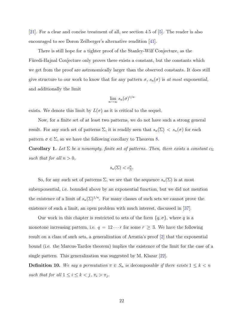
Now, for a finite set of at least two patterns, we do not have such a strong general
result. For any such set of patterns Σ, it is readily seen that sn(Σ) < sn(σ) for each
pattern σ ∈ Σ, so we have the following corollary to Theorem 8.
Corollary 1. Let Σ be a nonempty, finite set of patterns. Then, there exists a constant cΣ
such that for all n > 0,
sn(Σ) < cnΣ.
So, for any such set of patterns Σ, we see that the sequence sn(Σ) is at most
subexponential, i.e. bounded above by an exponential function, but we did not mention
the existence of a limit of sn(Σ)1/n. For many classes of such sets we cannot prove the
existence of such a limit, an open problem with much interest, discussed in [37].
Our work in this chapter is restricted to sets of the form q, σ, where q is a
monotone increasing pattern, i.e. q = 12 · · · r for some r ≥ 3. We have the following
result on a class of such sets, a generalization of Arratia’s proof [2] that the exponential
bound (i.e. the Marcus-Tardos theorem) implies the existence of the limit for the case of a
single pattern. This generalization was suggested by M. Klazar [22].
Definition 10. We say a permutation π ∈ Sn is decomposable if there exists 1 ≤ k < n
such that for all 1 ≤ i ≤ k < j, πi > πj.
22

Lemma 3. Let q = 12 · · · r and σ ∈ Sm for some r ≥ 3 and m ≥ 3. Then, if σ is not
decomposable, the limit [
L(q, σ) = limn→∞
sn(q, σ)1/n
exists.
Proof. Let m, n ≥ 1. For each pair of permutations α ∈ Sm(q, σ) and β ∈ Sn(q, σ),
construct the (m + n)-permutation
π = (α1 + n) (α2 + n) · · · (αm + n) β1 β2 · · · βn.
By our assumptions on α and β, π avoids q and σ in its first m entries and in its last n
entries. Furthermore, as q and σ are not decomposable, there is no copy of q or σ which
contains entries from these two sets. Thus, π is (q, σ)-avoiding and uniquely determined by
α and β, proving the following inequality.
sm+n(q, σ) ≥ sm(q, σ)sn(q, σ).
We have the following lemma by Fekete [17] for superadditive sequences. The analog of
this lemma for subadditive sequences was used in Arratia’s proof for the case of a single
pattern.
Lemma 4 (Fekete). For every sequence ann∈N satisfying
an+m ≥ anam
for all m,n ≥ 0, the limit
limn→∞
an
n
exists.
Applying Fekete’s lemma to the sequence log sn(q, σ), we thus have that the sequence
sn(q, σ)1/n has a limit. As this sequence is bounded above, this limit is finite.
With these facts in mind, we define L on sets of two patterns as follows.
23

Definition 11. Let σ and τ be patterns. Then, define the following quality.
L(q, σ) = lim supn→∞
sn(σ, τ)1/n.
Of course, for pairs of patterns σ and τ for which the limit exists, such as those in
Lemma 3, the limit and lim sup agree, and L is as we want it to be.
2.2 An Open Problem by M. Atkinson
This work was originated in response to a question posed by Michael Atkinson at
the fifth International Conference on Pattern Avoiding Permutations. We answer the
question in the affirmative for all increasing patterns q on some classes of patterns σ and
specifically for q = 123 for larger classes of patterns σ.
For a pattern σ of length m, define σ′ to be the pattern (m + 1)σ. For example, for
σ = 2431, we have σ′ = 52431. Given a monotone ascending pattern q and a pattern σ,
does it hold that L(q, σ′) = L(q, σ)?
In any permutation the entries preceding the first ascendee form a decreasing
sequence. For a permutation π, if the first ascendee of π is the index i, we call πi the
threshold of π and call the decreasing sequence preceding the threshold the front end. The
set of entries following the threshold we call the back end.
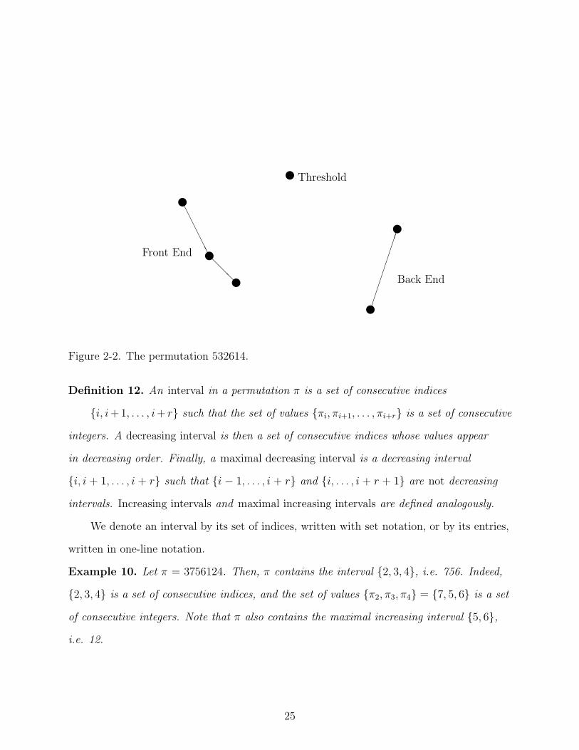
Example 9. For π = 532614, our first ascendee is the index 4, so the threshold of π is the
entry π4 = 6, the front end is 532, and the back end is 14, as shown in Figure 2-2.
Note that in our previous example each entry of the back end is less than the
threshold. Creating our own good luck, we chose 532614 for our example specifically
because it avoids 123. In fact, every 123-avoiding permutation shares this property,
a simple structure of which we shall take great advantage in our handling of these
permutations. To see this property, suppose our threshold is πt and there is an entry
πj in the back end (equivalently j > t) with πj > πt. By definition of ascendee, πt−1 < πt,
and the subsequence πt−1 πt πj forms a 123.
We borrow the next few definitions from the recent paper by Vatter [37].
24
x
x
x
AAAAAA@
@@
Front End
xThreshold
x
x
£££££££££
Back End
Figure 2-2. The permutation 532614.
Definition 12. An interval in a permutation π is a set of consecutive indices
i, i +1, . . . , i+ r such that the set of values πi, πi+1, . . . , πi+r is a set of consecutive
integers. A decreasing interval is then a set of consecutive indices whose values appear
in decreasing order. Finally, a maximal decreasing interval is a decreasing interval
i, i + 1, . . . , i + r such that i − 1, . . . , i + r and i, . . . , i + r + 1 are not decreasing
intervals. Increasing intervals and maximal increasing intervals are defined analogously.
We denote an interval by its set of indices, written with set notation, or by its entries,
written in one-line notation.
Example 10. Let π = 3756124. Then, π contains the interval 2, 3, 4, i.e. 756. Indeed,
2, 3, 4 is a set of consecutive indices, and the set of values π2, π3, π4 = 7, 5, 6 is a set
of consecutive integers. Note that π also contains the maximal increasing interval 5, 6,i.e. 12.
25

Definition 13. Given a permutation π ∈ Sn with interval I = i, i + 1, . . . , i + r, we
define the deflation of π at I to be the reduction of π1 · · · πi−1 πi πi+r+1 · · · πn. Similarly,
the inflation of π at the index i by the permutation σ ∈ Sm is the permutation obtained
from π by increasing by m − 1 each entry greater than πi and replacing the entry πi with
the interval whose reduction is σ.
Example 11. The deflation of the permutation 264513 at the interval 645 is the reduction
is 2413. The inflation of the permutation 3124 at index 3 by the permutation 321 is
514326.
It was remarked above that the front end of a permutation is monotone decreasing.
Thus, the front end has a unique factorization as the concatenation of one or more
maximal decreasing intervals.
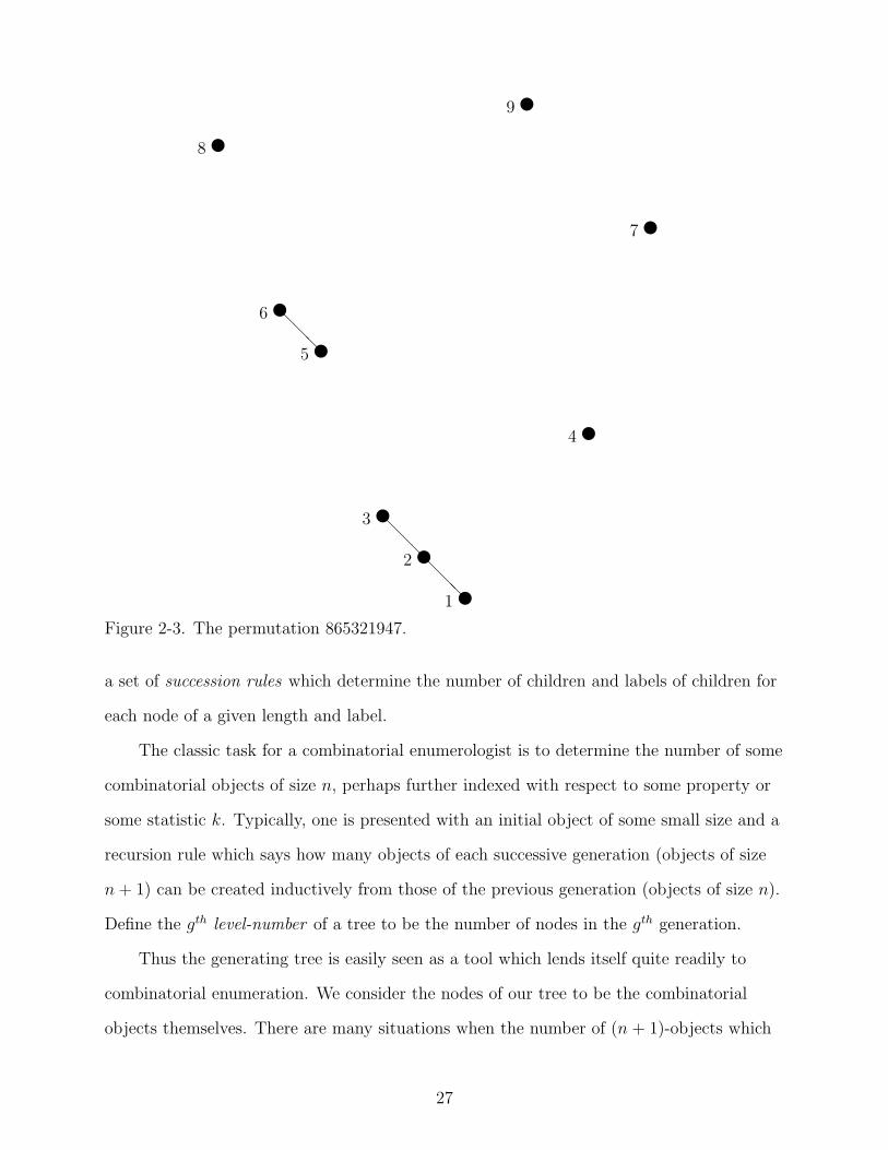
Example 12. Let π = 865321947. Then, the front end of π is 865321, the concatenation
of maximal decreasing intervals 8, 65, and 321.
2.3 Generating Trees
A tree is simply a connected, acyclic simple graph, or equivalently a connected simple
graph on n vertices with n − 1 edges. A forest is a collection of trees. A rooted, labeled
tree is a tree with an assignment of labels (typically non-negative integers) to the nodes
and one node designated the root, giving an orientation to the entire graph. We say that
a node y is a child of the node x if the final edge in the unique path from the root to y
is the edge x, y. Likewise, we call x the parent of y and define the depth of y to be the
number of children. The descendants of y is the set of nodes x such that the unique path
from the root to x passes through y. Finally, we call the set of all nodes whose unique
path to the root contains k edges the kth generation of the tree.
In [39] Julian West defines a generating tree as a rooted, labeled tree having the
property that the labels of the children of each node x can be determined from the label of
x itself. This leads to the characterization of a generating tree by the label of its root and
26
x
x
x
x
x
x
x
x
x
@@
@
@@
@@
@@
8
6
5
3
2
1
9
4
7
Figure 2-3. The permutation 865321947.
a set of succession rules which determine the number of children and labels of children for
each node of a given length and label.
The classic task for a combinatorial enumerologist is to determine the number of some
combinatorial objects of size n, perhaps further indexed with respect to some property or
some statistic k. Typically, one is presented with an initial object of some small size and a
recursion rule which says how many objects of each successive generation (objects of size
n + 1) can be created inductively from those of the previous generation (objects of size n).
Define the gth level-number of a tree to be the number of nodes in the gth generation.
Thus the generating tree is easily seen as a tool which lends itself quite readily to
combinatorial enumeration. We consider the nodes of our tree to be the combinatorial
objects themselves. There are many situations when the number of (n + 1)-objects which
27

x
x
x
x x x
x
´´
´´
´´
´´
QQQ´
´´
´´
´´
´
QQQ
root
parent
children
third generation of tree
Figure 2-4. A rooted tree.
can be generated from any n-object is all we need to know, so we might as well label each
node with its depth.
In [39] West begins with a trivial example, the complete binary tree. We begin with a
root with label (2). Our succession rule is that each node with label (2) has two children
also labeled (2).
Example 13 ([39], Example 1). The complete binary tree is determined by the set of rules
Root : (2)
Rule : (2) → (2)(2)
A long celebrated integer sequence is that of the Fibonacci numbers (Fn)n≥0 =
0, 1, 1, 2, 3, 5, . . ., where we have the initial assumptions F0 = 0 and F1 = F2 = 1, and each
additional number Fn is the sum of the preceding two numbers of the sequence. They will
play a role in our studies of pattern avoidance, so we show their generating tree as a less
trivial example of generating trees and a slow introduction to this sequence.
28

(2)
(2) (2)
(2) (2) (2) (2)
%%
%%
%%
%%
ee
ee
ee
ee
¢¢
¢¢
¢¢
¢¢
AAAAAAAA
¢¢
¢¢
¢¢
¢¢
AAAAAAAA
qqq
qqq
qqq
qqq
Figure 2-5. The complete binary tree.
Example 14 ([39], Example 3). The Fibonacci tree is determined by the set of rules
Root : (1)
Rules : (1) → (2)
(2) → (1)(2)
The observant reader undoubtedly noticed that our succession rules are not the same as the
recursion we gave to define our sequence. We verify that these rules are in fact equivalent
to the statement Fn+1 = Fn + Fn−1. For each n ≥ 1 we have a set of G(2)n objects labeled
(2) and a set of G(1)n objects labeled (1). Each object in either set produces an offspring of
size n + 1 with label (2). So, we have
G(2)n+1 = G(1)
n + G(2)n = Fn.
Furthermore, each object in G(1)n produces an offspring of size n + 1 with label (1), so
G(1)n+1 = G(2)
n = Fn−1.
where the second equality follows from our previous statement. We have thus accounted for
all Fn+1 objects, and we have our recurrence.
29

(1)
(2)
(1) (2)
(2) (1) (2)
%%
%%
%%
%%
ee
ee
ee
ee
¢¢
¢¢
¢¢
¢¢
AAAAAAAA
qqq
qqq
qqq
Figure 2-6. The Fibonacci tree.
For a detailed exposition on the use of generating trees in the study of pattern
avoidance, see [39], [12], [36], [10] and [24].
Here we define the generating trees which will be used throughout. These definitions
depend on the patterns σ and q which are being avoided, so we assume the patterns to
be given. This will be clear from context. First we explain the motivations. Recall our
′ notation. For a pattern σ ∈ Sm, the pattern σ′ ∈ Sm+1 is obtained by prepending σ
with the entry (m + 1). The fundamental question here is whether various limits (or
limit suprema) for the number of permutations which avoid some pattern σ are the same
as those which avoid σ′ (assuming for now that the limits exist). It was noted above
that σ-avoidance implies σ′-avoidance, but there are σ′ avoiders which contain σ. So,
our question boils down to just how many of these there are, in particular what are
the asymptotics of these permutations with respect to the set of σ-avoiders. We would
30
like to make use of generating trees to study the set of σ′-avoiders which contain σ, i.e.
π : π avoids σ′ \ π : π avoids σ.For each n ≥ 0, let Tn = Tn(q, σ) be the set of all (q, σ)-avoiding permutations of
length n, enumerated by tn. We construct the generating tree T = T (q, σ) whose nth level
is Tn. A permutation π ∈ Tn+1 is a child of γ ∈ Tn if and only if π can be obtained by
inserting n + 1 at one of the n + 1 open sites in γ. Similarly, for each n ≥ 0, let Un be
the set of all (q, σ′)-avoiding permutations of length n, enumerated by un, and construct
the generating tree U = U(q, σ) with levels Un and succession defined as for T . Atkinson’s
question is thus answered in the affirmative for some pattern by showing that un does
not grow asymptotically faster than tn. We will focus our attention on the sets Wn of
all (q, σ′)-avoiding permutations of length n which contain at least one copy of σ, i.e.
Wn = Un\Tn, enumerated by wn. This motivates the forest W = U\T . Note that each
tree in W is rooted at a q-avoiding permutation which avoids σ′ and contains σ but whose
parent in U avoids σ. For q = 123 and σ = 132, we have the tree shown in Figure 2-7.
An active site in a permutation is a valid insertion point, that is, a site where we
can insert n + 1 and obtain a child which is still in the current generating tree, so for
our purposes an active site is such that the insertion will not cause an occurence of any
pattern which we seek to avoid. The depth of a permutation π is the number of active
sites in π, equivalent to the notion of depth defined above on generating trees. We note
that the depth depends on both the permutation itself and on the tree, specifically the
pattern being avoided which determines the tree.
2.4 “Hat” Notation
Given a permutation π and a pattern σ, we denote by σ any copy of σ in π. For
each index p, we use the notation σp to refer to an entry which serves the role of σp in
some σ. As there may be more than one copy of the pattern σ in some permutation, σp
generally does not refer to any specific entry. For example, with σ = 132, the permutation
π = 24135 contains one σ, namely 243. In this case σ1 refers to the entry π1 = 2, σ2 refers
31

1 (2)%
%%
%%
%%%
21 (3)¡
¡¡
¡¡
¡¡¡
321 (4)¡
¡¡
¡¡
¡¡¡
4321 (5)
££
££
££
££3421 (1)
BBBBBBBB
3241 (1)
@@
@@
@@
@@3214 (1)
BBBBBBBB231 (1)
4231 (2)
@@
@@
@@
@@213 (1)
4213 (2)
ee
ee
ee
ee12 (2)
BBBBBBBB312 (2)£
££
££
£££
4312 (3)
BBBBBBBB3412 (1)
qqq
qqq
qqq
qqq
qqq
qqq
qqq
qqq
Figure 2-7. T(123,132).
to π2 = 4, and σ3 refers to π4 = 3. On the other hand, the permutation 1432 contains
three σ’s, namely 143, 142, and 132. In this case we can refer to the σ1, the entry 1, but
we have several σ2’s and several σ3’s. It should also be noted that one entry could be both
a σi and a σj for some i 6= j.
Example 15. With σ = 132, in the permutation π = 25431, π3 = 4 is the σ2 = 3 of the
subsequence 254 as well as the σ3 = 2 of the subsequence 243.
Often we will determine the depth of a permutation π by the index of the rightmost
σ1 in π, by which we mean the entry with the greatest index of those entries πk such that
there exists a σ which begins at πk.
Example 16. For σ = 231 and π = 43521, the entries π1 and π2 are both σ1’s, and we call
π2 the rightmost σ1.
32

Any confusion over hat notation should fade upon seeing its motivation in the
following proofs. As long as we use the ˆ notation carefully, the meaning should always be
clear.
2.5 Monotone Increasing Patterns q
For any pattern σ we have by construction that σ′ contains σ, so it follows immediately
from our introductory remarks on pattern avoidance that
sn(σ) ≤ sn(σ′).
for all n, and
L(σ) ≤ L(σ′).
Of course, these bounds also extend to
L(σ, Π) ≤ L(σ′, Π).
for any set of patterns Π, etc.
Let q be the increasing pattern 123 · · · r. We will show that the statement L(q, σ′) =
L(q, σ) holds if a pattern σ begins with its greatest entry. Our proof builds on Bona’s
proof for the case of single patterns, found in [4].
Definition 14. A left-to-right maximum is an entry in a permutation which is greater
than each entry to its left. The remaining entries of a permutation are those which are
not left-to-right maxima . A weak class (weak n-class) is a set of permutations (resp.
n-permutations) whose left-to-right maxima are the same and are in the same respective
positions.
Example 17. The permutations 32415 and 31425 both have left-to-right maxima 3, 4, and
5, at the first, third, and fifth entries, so we say that 32415 and 31425 are in the same
weak class or weak 5-class.
33

Example 18. The permutations 3412 and 2413 both have left-to-right maxima in the first
two positions, but as the maxima themselves are not the same, 3412 and 2413 are not in
the same weak 4-class.
Lemma 5. For each r ≥ 1, there exists a polynomial fr(x) such that for all n ≥ 1 the
number of weak n-classes of permutations with exactly r left-to-right maxima is less than
fr(n).
Proof. Fix n. We can easily count the weak n-classes with one or two left-to-right
maxima. An n-permutation with only one left-to-right maximum must begin with n,
so there is only one such weak n-class. Next we claim that there are(
n2
)weak n-classes
with exactly two left-to-right maxima. Indeed, pick two numbers a, b ∈ [n] with a < b.
Place the entry a in the first position, and place the entry n in the (n + 1 − b)th position.
Given such constraints, we can always place the remaining entries to find at least one
permutation in each weak n-class. For r > 2 we take the same approach but allow
overcounting. There are at most(
nr
)2ways to choose the entries and positions (numerical
and geographical values) for the r left-to-right maxima, as this includes all possible
sequences of left-to-right maxima, as well as some sequences which cannot possibly be the
set of left-to-right maxima of a permutation. As(
nr
)2is a polynomial in n for any fixed r,
the statement holds.
Corollary 2. For each r ≥ 1, the number of weak n-classes with less than r left-to-right
maxima is bounded by a polynomial in n.
Proof. For each 1 ≤ k < r, we have a polynomial upper bound fk(n) on the number of
weak n-classes with exactly k left-to-right maxima. The sum over all such k is clearly an
upper bound for the number of weak n-classes with fewer than r left-to-right maxima. As
a sum of (a fixed number of) polynomials is a polynomial, we are finished.
34

Proposition 19. Let q be the ascending pattern 1 2 · · · r, and let σ be a permutation which
begins with its greatest entry. Then,
L(q, σ′) = L(q, σ).
Proof. We first note that a permutation which avoids q has fewer than r left-to-right
maxima. Now, if a permutation avoids σ′, then its remaining entries avoid σ. Indeed, by
definition each remaining entry is preceded by a left-to-right maximum. If the remaining
entries of a permutation contain σ, then we may prepend this σ with any left-to-right
maximum which is to the left of and greater than σ1 to obtain a σ′, as σ1 is itself greater
than all other entries of σ by the fact that σ begins with its largest entry.
Therefore, we can overcount n-permutations which avoid σ′ by multiplying the
number of weak n-classes which have fewer than r left-to-right maxima by the number of
possible (q, σ)-avoiding permutations of the remaining entries. By Corollary 2 the number
of such weak n-classes is at most a polynomial function f(n). Therefore our overcount of
n-permutations is f(n)sn−1(q, σ). We are now in position to take our limits.
L(q, σ′) = lim supn→∞
sn(q, σ′)1/n
≤ lim supn→∞
(f(n)sn−1(q, σ))1/n
= lim supn→∞
f(n)1/nsn−1(q, σ)1/n
= lim supn→∞
1 · sn−1(q, σ)1/n
= L(q, σ).
Combined with the knowledge that L(q, σ′) ≥ L(q, σ), we are finished.
The following lemma from [4] and [5] provides an upper bound on the number of
permutations of length n which avoid the increasing pattern of length r.
35

Lemma 6. sn(1 2 · · · r) ≤ (r − 1)2n for all r, n ≥ 2.
Proof. We define a rank function on the entries of each permutation π ∈ Sn(12 · · · r) by
setting the rank of an entry πi to be the length of any maximal increasing subsequence
πj1πj2 · · · πi. Note that this generalizes the concept of the left-to-right-maxima, which are
precisely those entries with rank 1.
If an entry πi has rank t, then there exists some increasing subsequence πj1πj2 · · · πjt−1πi
of length t, so for any entry πk > πi with k > i, the rank of πk is at least t + 1, as we have
the increasing subsequence πj1πj2 · · · πjt−1πiπk. Therefore, for each 1 ≤ t ≤ n, we see that
the entries of rank t form a decreasing sequence.
There are at most n such decreasing sequences, and as sets of indices they form a
set partition of [n]. As π is assumed to be 12 · · · r-avoiding, π has no entry of rank r or
greater, and there are at most r − 1 blocks of our set partition. Assigning each entry of π
to one of r − 1 blocks, we may overcount and see that there are at most (r − 1)n possible
assignments of the indices to the blocks and at most (r − 1)n possible assignments of the
values to the blocks.
With this lemma in hand, we subtly alter another proof of Bona to achieve:
Proposition 20. Let q be the ascending pattern 1 2 · · · r, let σ be a pattern, and let c be a
constant such that for all n ≥ 1, sn(q, σ) ≤ cn. Then, for all n ≥ 1,
sn(q, σ′) ≤ (c + (r − 2)2)n−1.
Proof. In order for a permutation to avoid σ′, it is necessary that it avoid σ in the region
to the right of n. So, we may overcount the number of (q, σ′)-avoiding permutations
by choosing where to place n, which entries to place to the left of n such that they are
1 2 · · · (r − 1)-avoiding (because any 1 2 · · · ( ˆr − 1) among them could be postpended
with n to create a q), and how to arrange the entries to the right of n such that they
are (q, σ)-avoiding. We let k be the position of n, so there are(
n−1k−1
)possibilities for the
entries preceding n. By Lemma 6 there are at most (r − 1)2(k−1) possible permutations
36
of these entries. Finally, by our original hypothesis on Sn(q, σ), there are at most cn−k
possible permutations of the n − k entries which follow n. Altogether, these work out to
the binomial expansion
sn(q, σ′) ≤n∑
k=1
(n− 1
k − 1
)(r − 2)2(k−1)cn−k
= (c + (r − 2)2)n−1,
concluding the proof.
In particular, for q = 123, we have (r−2)2 = 1, so with the assumption sn(123, σ) ≤ cn
for all n, we find sn(123, σ′) ≤ (c + 1)n−1 for all n.
The Stanley-Wilf Conjecture (Marcus-Tardos Theorem) tells us that for any pattern
σ or set of patterns Σ there is such a constant c as in the above hypothesis. In the case of
avoiding a single pattern σ, Arratia showed in [2] that the sequence sn(σ)1/n is increasing.
However, there are sets of patterns Σ for which the sequence sn(Σ)1/n is not increasing.
Thus, taking c to be the least constant such that sn(Σ) ≤ cn for all n < N for some N , it
may be that there is a constant d < c such that sn(Σ) ≤ dn for all n > N . In particular,
the constant c may be significantly greater than L(Σ), so the new constant d is closer to
our limit and thus a better indicator of the asymptotic behavior of our sequence sn(Σ).
Such a situation motivates a strengthening of the previous proposition.
Proposition 21. Let q be the ascending pattern 1 2 · · · r, let σ be a pattern, and let d be a
constant such that for some N and all n ≥ N, sn(q, σ) ≤ dn. Then, there exists a constant
D such that, for all n ≥ N ,
sn(q, σ′) ≤ D(d + (r − 2)2)n−1.
Proof. The set sn(q, σ) : 1 ≤ n < N is finite, so it is bounded above, and we can choose
a constant D such that sn(q, σ) < Ddn for all 1 ≤ n < N . We retain all machinery from
the proof of the previous proposition, except instead of counting at most cn−k possible
37
permutations of the n − k entries which follow n, we count them by Ddn−k. Then our
expansion becomes
sn(q, σ′) ≤n∑
k=1
(n− 1
k − 1
)(r − 2)2(k−1)Ddn−k
= D
n∑
k=1
(n− 1
k − 1
)(r − 2)2(k−1)dn−k
= D(d + (r − 2)2)n−1.
2.6 The Pattern q = 123
In this section we restrict our attention to the 123-avoiding environment. Some
statements will be generalized to longer ascending patterns q in the following section.
Consider the active sites of a permutation π ∈ W . As any child of π is 123-avoiding,
there can be no active site to the right of the first ascendee. As any child of π is
σ′-avoiding, there can be no active site to the left of a σ1. However, the consecutive
sites satisfying these two criteria are all active. So, our understanding of depth reduces
to understanding where these two bounds lie. Furthermore, if π has depth d, inserting
n + 1 into one of the d active sites will not increase the depth. Indeed, n + 1 is inserted
to the left of the first ascendee of π and itself becomes the first ascendee in the child.
The rightmost σ1 of π remains in place in the child, so the child will have a rightmost σ1
which is at the same position or to the right of that of π. This demonstrates the following
lemma. Recall our definition of the threshold of a permutation as the leftmost ascendee of
the permutation.
Lemma 7. Let π ∈ W for some pattern σ. Then, the depth of π is the distance from the
righmost σ1 to the threshold, i.e. the difference of the index of the threshold and the index
of the rightmost σ1.
38

We proceed with a lemma which will be used extensively as it provides a polynomial
bound for the level-numbers of each tree in the forest W .
Lemma 8. Let σ be a pattern of length m which does not begin with m. Let π be a
(123, σ′)-avoiding permutation with depth d which contains σ but whose parent avoids σ.
Then, the number of descendants of π at the jth generation, i.e. the jth level-number of the
tree in W rooted at π, is bounded above by
(d + j
d
),
which is a polynomial in j of degree d.
Proof. (We are in fact bounded by the lesser polynomial(
d+j−1d−1
), however we dropped the
−1’s for neatness.) Let n be the length of π. First we note that π does not begin with n.
Indeed, as the parent of π has no σ but π has a σ, n is the m in any σ in π. π contains a
copy of σ, which does not begin with its largest entry, so n appearing to the left of any σ
would complete a σ′, contradicting the assumption that π is σ′-avoiding. In fact, by this
argument we see that n is the threshold and σ must contain entries in the front end of π.
We are trying to show that the number of descendants at each generation is bounded
by our polynomial, so we might as well assume the worst case scenario, that inserting at
the kth active site always produces a child of depth k, i.e. that the rightmost σ1 of a child
is always at the same position as the rightmost σ1 of the parent. Then, for all 1 ≤ k ≤ d,
we in fact have the succession rules
Root : (d)
Rule : (k) → (1)(2) · · · (k)
An example of a tree in such a forest is shown in Figure 2-8.
39

42153 (3)´
´´
´´
´´
´´
´´
462153 (1)
4762153qqq
426153 (2)¢
¢¢
¢¢
¢¢¢
4726153qqq
AAAAAAAA
4276153qqq
QQ421653 (3)
¢¢
¢¢
¢¢
¢¢4721653
qqq
BBBBBBBB
4271653qqq
@@
@@
@@
@@4217653qqq
Figure 2-8. Tree in W(123,231) rooted at 42153
Denoting by aj,k the number of permutations at the jth level with depth k, 0 ≤ j and
1 ≤ k ≤ d, we have the recursive system
a0,d = 1
a0,k = 0 ∀k 6= d
aj,k =d∑
t=k
aj−1,t ∀j ≥ 1, 1 ≤ k ≤ d.
From this recursive system we see that aj,k =(
d−k+1+jd−k+1
). For each d and j we may
sum over all k to attain the level-number(
d+j−1d−1
). However, a combinatorial proof is
preferable. We know that(
d+j−1d−1
)counts j-multisets of [d], and such a multiset written in
nonincreasing order spells out the order of active sites chosen in the lineage from π to a
permutation of length n + j.
40

Definition 15. ([5] Definition 5.33) A permutation π is called layered if it can be written
as the concatenation q1q2 · · · qk where each qi is a decreasing sequence of consecutive
integers and the leading entry of qi is smaller than the leading entry of qi+1 for 1 ≤ i ≤k − 1.
Example 22. An example of a layered permutation is 213654, which has three layers, as
shown in Figure 2-9.
x2
x1
x3
x6
x5
x4
@@
@@
@@¢
¢¢¢¢¢¢¢¢¢¢¢
££££££££££££££££££@
@@
@@
@@
@@
@@
@
Figure 2-9. The layered permutation 213654 with layers 21, 3, and 654
Many results are known concerning pattern avoidance and pattern packing for layered
permutations. One can see Section 5.2.2 of [5], [27], [6], and [20]. Our next result is on
layered patterns with just two layers, equivalently non-monotone layered patterns which
avoid 123.
Proposition 23. Let σ be a pattern of the form
d (d− 1) · · · 1 m (m− 1) · · · (d + 1)
41

for some d ≥ 1. Then,
L(123, σ′) = L(123, σ).
Proof. Note that any permutation which contains σ has depth at most d. In fact, we will
use a stronger property of the roots of the trees in W in which the depth is exactly d.
Indeed, let the N -permutation ρ be such a root. We know that ρ contains at least one
copy of σ, while the parent of ρ in U avoids σ. As the only change between the parent
of ρ and ρ is the insertion of N , N must act as m in any σ in ρ. This implies that there
is a set of d entries preceding N which serve as the d, ˆ(d− 1), . . . , 1 in a σ in ρ. In fact,
as the front ends of both σ and ρ are decreasing (because σ and ρ are 123-avoiding),
and as every front end entry of σ is less than every back end entry of σ, the d entries
immediately preceding N serve these roles. Therefore, the rightmost σ1 cannot be more
than d positions to the left of N . As N is the only m in ρ, the entry which is d positions
to the left of N is clearly the rightmost σ1.
That there is a fixed depth which applies to every root in W makes our job easy.
For each N , the total number of trees in W whose roots have length N is less than
NuN−1, as each such root in W has a parent in U on the (N − 1)st level of U , and an
(N − 1)-permutation can have depth at most N . Each such tree has level-numbers which
are bounded above by the polynomial(
d+n−N−1d−1
). So, the nth level-number of W , wn, is
bounded by
42
wn
n∑N=m
NuN−1
(d + n−N − 1
d− 1
)
≤ un
n∑N=m
N
(d + n−N − 1
d− 1
)
≤ un
n∑N=m
n
(d + n−m− 1
d− 1
)
≤ unn2
(d + n−m− 1
d− 1
),
un times a fixed polynomial f(n), a polynomial which only depends on σ. With the fact
that sn(123, σ) ≤ sn(123, σ′) for all n, we have
u1/nn ≤ w1/n
n ≤ u1/nn (f(n))1/n .
The nth roots of this fixed polynomial approach 1, so we may apply the Squeeze Theorem
to achieve
lim supn→∞
w1/nn = lim sup
n→∞u1/n
n .
We just saw that, if the front end is composed of entries which are all lower than
any entry in the back end, then there is a polynomial function which depends only on the
pattern and dictates the number of descendants for any permutation. Now consider how
the situation changes if there is more than one maximal decreasing interval in the front
end. Our shortest and prototypical example is 3142. The critical difference here is that
our depth is no longer bounded as it was for the patterns considered in Proposition 23.
For example, for any d > 2, we have the (123, 3142)-avoiding permutation (d + 1) (d −1) (d − 2) · · · 1 (d + 2) d, which has depth d. This means we can are not guaranteed a
fixed bound to the degrees of our generating polynomials of the level-numbers of our trees.
All is not lost, however, as we can show that for any of a class of patterns σ and any k
there is an upper bound to the number of trees in W whose root has depth which is k
43

less than its length. For the pattern 3142 it follows easily from the fact that the depth
of a permutation in W is completely determined by the length of the second maximal
decreasing interval in the front end. First, we calculate L(123, 3142).
As was mentioned in our introduction to generating trees, a famous combinatorial
sequence is the Fibonacci numbers Fn defined for all n ≥ 0 by the recursive system
F0 = 0
F1 = 1
Fn+1 = Fn + Fn−1 ∀ n ≥ 1.
Multiplying both sides of the recursive equation Fn+1 = Fn + Fn−1 by xn, summing
over all n ≥ 1, and solving for the ordinary generating function F (x) =∑
n≥0 Fnxn, we
find
F (x) =x
1− x− x2=
∑n≥0
1√5
((1 +
√5
2
)n
−(
1−√5
2
)n),
from which we see that Fn is asymptotically approximated by the nth power of the
dominant term, the golden ratio,
Fn ∼(
1 +√
5
2
)n
.
Furthermore, as the golden ratio enjoys the property of being a solution to the equation
x2 = x + 1, so that(
1+√
52
)2
= 1+√
52
+ 1 = 3+√
52
, we immediately achieve an approximation
for every other Fibonacci number
F2n+1 ∼(
3 +√
5
2
)n
.
44
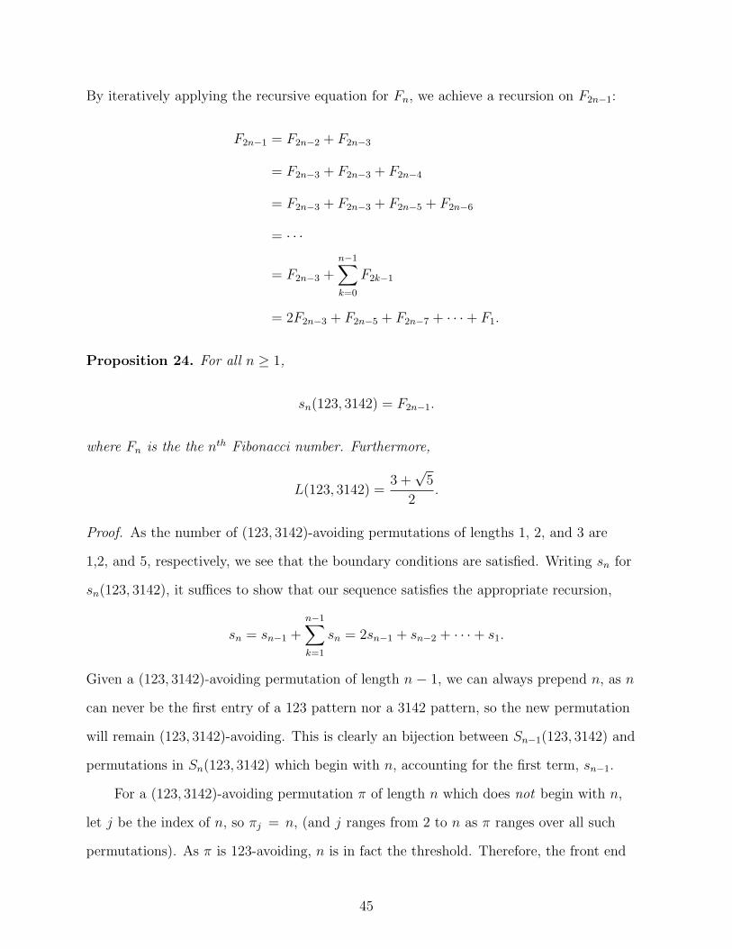
By iteratively applying the recursive equation for Fn, we achieve a recursion on F2n−1:
F2n−1 = F2n−2 + F2n−3
= F2n−3 + F2n−3 + F2n−4
= F2n−3 + F2n−3 + F2n−5 + F2n−6
= · · ·
= F2n−3 +n−1∑
k=0
F2k−1
= 2F2n−3 + F2n−5 + F2n−7 + · · ·+ F1.
Proposition 24. For all n ≥ 1,
sn(123, 3142) = F2n−1.
where Fn is the the nth Fibonacci number. Furthermore,
L(123, 3142) =3 +
√5
2.
Proof. As the number of (123, 3142)-avoiding permutations of lengths 1, 2, and 3 are
1,2, and 5, respectively, we see that the boundary conditions are satisfied. Writing sn for
sn(123, 3142), it suffices to show that our sequence satisfies the appropriate recursion,
sn = sn−1 +n−1∑
k=1
sn = 2sn−1 + sn−2 + · · ·+ s1.
Given a (123, 3142)-avoiding permutation of length n − 1, we can always prepend n, as n
can never be the first entry of a 123 pattern nor a 3142 pattern, so the new permutation
will remain (123, 3142)-avoiding. This is clearly an bijection between Sn−1(123, 3142) and
permutations in Sn(123, 3142) which begin with n, accounting for the first term, sn−1.
For a (123, 3142)-avoiding permutation π of length n which does not begin with n,
let j be the index of n, so πj = n, (and j ranges from 2 to n as π ranges over all such
permutations). As π is 123-avoiding, n is in fact the threshold. Therefore, the front end
45
of π consists of one maximal decreasing interval. Indeed, if the front end contains more
than one maximal decreasing interval, then there exist entries in the front end πi and πi+1,
with the entry (πi+1 − 1) in the back end, and the reduction of πi πi+1 n (πi − 1) is 3142,
contradicting our assumption on π.
As the front end of π is an interval, the deflation of π at the front end is a (123, 3142)-avoiding
permutation π of length n − j + 2. The largest entry of π is of course π2 = (n − j + 2).
Removing this entry, we obtain a (123, 3142)-avoiding permutation of length n − j + 1
(which may or may not begin with its largest entry).
We claim that this is a bijection. Indeed, given a permutation γ ∈ Sn−j+1(123, 3142),
the inflation of γ at the first index by the permutation (j − 1) (j − 2) · · · 1 is a
(123, 3142)-avoiding permutation γ of length n − 1. Inserting n at index j regains a
permutation in Sn(123, 3142), and this is an injection. Such a construction over all j
accounts for the terms sn−1 + · · ·+ s1 in our recursion.
The limit L(123, 3142) = 3+√
52
follows immediately from the above discussion of the
asymptotics of the Fibonacci numbers.
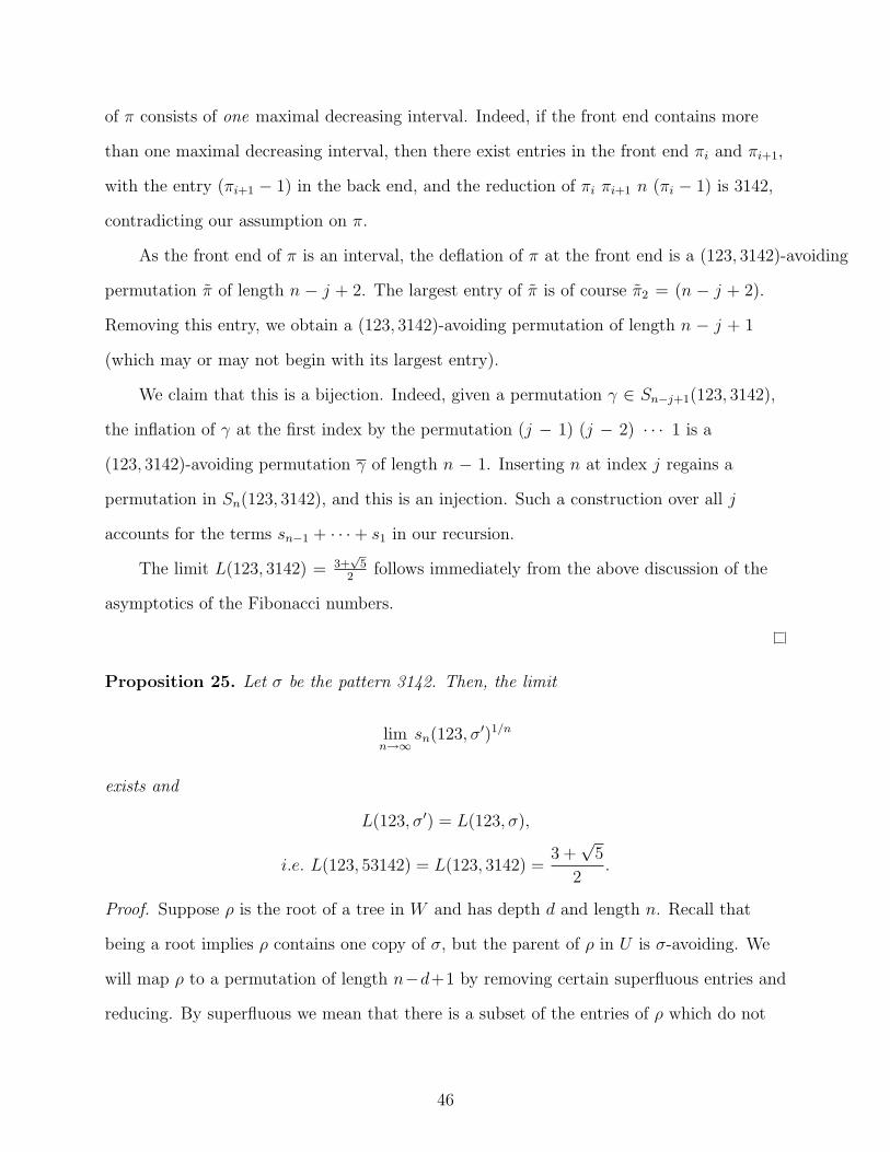
Proposition 25. Let σ be the pattern 3142. Then, the limit
limn→∞
sn(123, σ′)1/n
exists and
L(123, σ′) = L(123, σ),
i.e. L(123, 53142) = L(123, 3142) =3 +
√5
2.
Proof. Suppose ρ is the root of a tree in W and has depth d and length n. Recall that
being a root implies ρ contains one copy of σ, but the parent of ρ in U is σ-avoiding. We
will map ρ to a permutation of length n−d+1 by removing certain superfluous entries and
reducing. By superfluous we mean that there is a subset of the entries of ρ which do not
46
add any information to the identity of ρ in the sense that they are completely determined
by the other entries and the fact that ρ has length n and depth d.
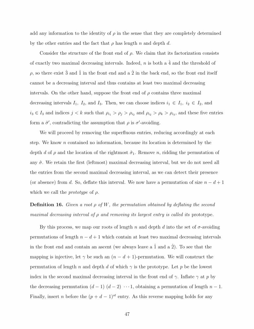
Consider the structure of the front end of ρ. We claim that its factorization consists
of exactly two maximal decreasing intervals. Indeed, n is both a 4 and the threshold of
ρ, so there exist 3 and 1 in the front end and a 2 in the back end, so the front end itself
cannot be a decreasing interval and thus contains at least two maximal decreasing
intervals. On the other hand, suppose the front end of ρ contains three maximal
decreasing intervals I1, I2, and I3. Then, we can choose indices i1 ∈ I1, i2 ∈ I2, and
i3 ∈ I3 and indices j < k such that ρi1 > ρj > ρi2 and ρi2 > ρk > ρi3 , and these five entries
form a σ′, contradicting the assumption that ρ is σ′-avoiding.
We will proceed by removing the superfluous entries, reducing accordingly at each
step. We know n contained no information, because its location is determined by the
depth d of ρ and the location of the rightmost σ1. Remove n, ridding the permutation of
any σ. We retain the first (leftmost) maximal decreasing interval, but we do not need all
the entries from the second maximal decreasing interval, as we can detect their presence
(or absence) from d. So, deflate this interval. We now have a permutation of size n− d + 1
which we call the prototype of ρ.
Definition 16. Given a root ρ of W , the permutation obtained by deflating the second
maximal decreasing interval of ρ and removing its largest entry is called its prototype.
By this process, we map our roots of length n and depth d into the set of σ-avoiding
permutations of length n − d + 1 which contain at least two maximal decreasing intervals
in the front end and contain an ascent (we always leave a 1 and a 2). To see that the
mapping is injective, let γ be such an (n − d + 1)-permutation. We will construct the
permutation of length n and depth d of which γ is the prototype. Let p be the lowest
index in the second maximal decreasing interval in the front end of γ. Inflate γ at p by
the decreasing permutation (d − 1) (d − 2) · · · 1, obtaining a permutation of length n − 1.
Finally, insert n before the (p + d − 1)st entry. As this reverse mapping holds for any
47

σ-avoiding permutation which contains an ascent and at least two maximal decreasing
intervals in its front end, we can overcount them as follows. We know that Sk(123, 3142)
is F2k−1, F2k−1 < βk for all k ≥ 1, and F1/k2k−1 → β, where β = (3 +
√5)/2. So, for any
N , the number of roots in W of length N and depth d is less than F2(N−d+1)−1 and, letting
k = N − d + 1 be the length of the prototype of each root, they each have level-number
polynomial
(d + j − 1
d− 1
)=
(N − k + 1 + j − 1
N − k + 1− 1
)
=
(N − k + j
N − k
)
=
(N − k + (n−N)
N − k
)
=
(n− k
N − k
).
We can now overcount all permutations in W by the roots of their trees and the
prototypes of the roots:
wn <
n−1∑
k=3
F2k−1
n∑
N=k+1
(n− k
N − k
)
<
n−1∑
k=3
F2k−12n−k
<
n−1∑
k=3
βk2n−k
<
n−1∑
k=3
βn
= (n− 3)βn.
In the end, we see that indeed the nth root approaches β = L(123, 3142).
48

As was mentioned prior to this proposition, the pattern 3142 makes our work easier
because the front end of the pattern itself is the concatenation two maximal decreasing
intervals. The above proof provided a warmup for the main result of this section. The
following lemma allows us to work with longer front ends.
Lemma 9. Let σ ∈ Sm be a pattern with a decreasing back end. Let ρ ∈ Sn be a root of
W . Then, the front end of ρ has at most m maximal decreasing intervals.
Proof. We first note that if i, i + 1, . . . , i + r is a maximal decreasing interval in the front
end of ρ, with i ≥ 2, then by maximality and the fact that the front end is decreasing,
ρi + 1 is in the back end of ρ.
Assume the front end of ρ has at least m + 1 maximal decreasing intervals. We show
that this implies the parent of ρ in U contains σ, a contradiction.
Label the rightmost m + 1 maximal decreasing intervals in the front end of ρ by
I1, I2, . . . , Im in order of their greatest entries. So, the front end of ρ is the concatenation
ρ1 · · · Im+1ImIm−1 · · · I1 or Im+1Im · · · I1 if ρ ∈ Im+1.
For each 1 ≤ i ≤ m, if the entry i is in the front end of σ, we choose an entry in Ii
to be our i. If the entry i is in the back end of σ, we choose an entry in the back end of ρ
which is greater than every entry of Ii and less than every entry of Ii+1 (if i < m) to be
our i. Doing so, we achieve our σ.
Example 26. If σ = 231, and ρ = 97642531, then our four labeled maximal decreasing
intervals are I1 = 2, I2 = 4, I3 = 76, and I4 = 9. Thus the front end of ρ is I4I3I2I1.
We construct our σ. As the entry 3 is greater than every entry of I1 and less than every
entry of I2, we choose 3 as our 1. Next we choose 4 as our 2. Finally, as 5 is greater than
every entry of I3 and less than every of I4, we choose 5 as our 3, and 453 indeed reduces
to σ = 231.
We now answer M. Atkinson’s question in the affirmative for patterns σ which avoid
123 and contain the entry 1 in the front end, noting that this restriction implies the back
49
end is decreasing. Any such pattern is not decomposable, so we do know that the limit L
exists and the sequence sn(123, σ)1/n is non-decreasing.
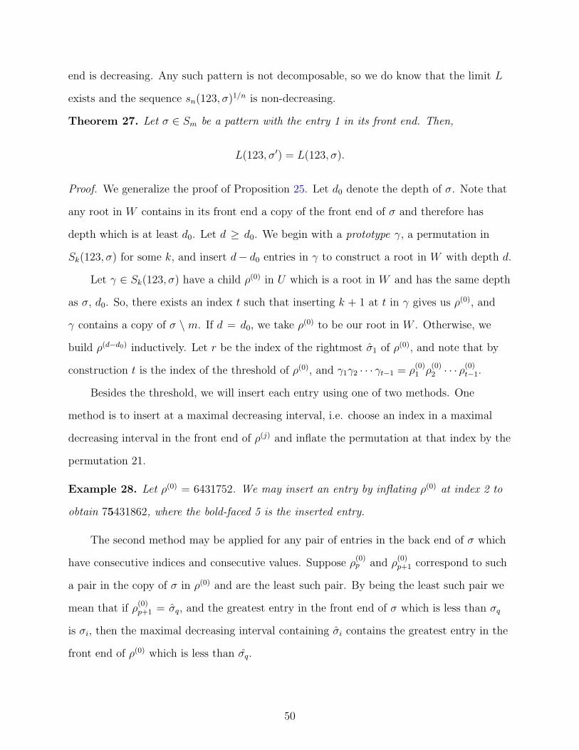
Theorem 27. Let σ ∈ Sm be a pattern with the entry 1 in its front end. Then,
L(123, σ′) = L(123, σ).
Proof. We generalize the proof of Proposition 25. Let d0 denote the depth of σ. Note that
any root in W contains in its front end a copy of the front end of σ and therefore has
depth which is at least d0. Let d ≥ d0. We begin with a prototype γ, a permutation in
Sk(123, σ) for some k, and insert d− d0 entries in γ to construct a root in W with depth d.
Let γ ∈ Sk(123, σ) have a child ρ(0) in U which is a root in W and has the same depth
as σ, d0. So, there exists an index t such that inserting k + 1 at t in γ gives us ρ(0), and
γ contains a copy of σ \ m. If d = d0, we take ρ(0) to be our root in W . Otherwise, we
build ρ(d−d0) inductively. Let r be the index of the rightmost σ1 of ρ(0), and note that by
construction t is the index of the threshold of ρ(0), and γ1γ2 · · · γt−1 = ρ(0)1 ρ
(0)2 · · · ρ(0)
t−1.
Besides the threshold, we will insert each entry using one of two methods. One
method is to insert at a maximal decreasing interval, i.e. choose an index in a maximal
decreasing interval in the front end of ρ(j) and inflate the permutation at that index by the
permutation 21.
Example 28. Let ρ(0) = 6431752. We may insert an entry by inflating ρ(0) at index 2 to
obtain 75431862, where the bold-faced 5 is the inserted entry.
The second method may be applied for any pair of entries in the back end of σ which
have consecutive indices and consecutive values. Suppose ρ(0)p and ρ
(0)p+1 correspond to such
a pair in the copy of σ in ρ(0) and are the least such pair. By being the least such pair we
mean that if ρ(0)p+1 = σq, and the greatest entry in the front end of σ which is less than σq
is σi, then the maximal decreasing interval containing σi contains the greatest entry in the
front end of ρ(0) which is less than σq.
50
As the depth of ρ(0) is the depth of σ, there is no entry in the front end of ρ(0) whose
value is between those of ρ(0)p and ρ
(0)p+1, so we have ρ
(0)p = ρ
(0)p+1 + 1. Let ρ
(0)i be the greatest
entry in the front end of ρ(0) which is less than ρ(0)p+1. Then, our second method of insertion
will be to insert the entry ρ(0)p at the index i and increase by one every entry which is at
least as large as ρ(0).
Example 29. Let σ = 41532 and ρ(0) = 521643. We may insert an entry in the front end
of ρ(0) to obtain 6421753, where the bold-faced 4 is the inserted entry.
Of course, in ρ(0) the pair ρ(0)p and ρ
(0)p+1 have consecutive values, and this may not
be the case in ρ(j) for greater values of j, as we may have already inserted at an index
q using the second method and corresponding to the pair ρ(0)p and ρ
(0)p+1. In this case, we
inflate ρ(j) at the index q by the permutation 21.
By Lemma 9, we know that the front end of ρ(0) has at most m maximal decreasing
intervals. In fact, there are exactly M maximal decreasing intervals in the subsequence
γr+1 · · · γt−1 for some M < m. Suppose there are P pairs of entries for which we may
apply our second method above, so altogether we have M + P choices for each insertion,
and we order them as C1, C2, . . . , CM+P . So, let x1, . . . , xd−d0 be a multiset of [M + P ]
with x1 ≥ x2 ≥ · · · ≥ xd−d0 . For each 1 ≤ j ≤ d − d0, inductively define ρ(j) to be
the insertion into ρ(j−1) determined by the choice Cxj. So, we obtain ρ(d−d0) by inserting
entries into some of the maximal decreasing intervals of ρ(0). As these entries were inserted
between the rightmost σ1 and the threshold, we have that ρ(j) has depth d0 + j for each j,
and each one is a root in W . Altogether, we obtain our root of depth d, ρ = ρ(d−d0).
Now, we have our root and we can overcount the (123, σ′)-avoiding permutations of
length n. We are in the same situation as in the proof of Proposition 25 except that we’ve
made(
M+P+d−d0−1M+P−1
)choices of how to insert the entries into our prototype to obtain our
root. Of course, M + P ≤ m and d− d0 < n, so this is bounded above by(
m+nm
). Note that
since σ contains the pattern 132, L(123, σ) ≥ L(123, 132) = 2. Altogether, we have
51

wn <
(m + n
m
) n−1∑
k=3
sk(123, σ)n∑
N=k+1
(n− k
N − k
)
<
(m + n
m
) n−1∑
k=3
sk(123, σ)2n−k
<
(m + n
m
) n−1∑
k=3
sn(123, σ)
=
(m + n
m
)(n− 3)sn(123, σ).
Taking the limit,
limn→∞
w1/nn ≤ lim
n→∞
(m + n
m
)1/n
(n− 3)1/nsn(123, σ)1/n
= limn→∞
sn(123, σ)1/n
= L(123, σ).
Experimental results support the following conjecture of Atkinson.
Conjecture 30. Let σ be any pattern. Then,
L(123, σ′) = L(123, σ).
52

CHAPTER 3PATTERN PACKING
3.1 General Pattern Packing
In the previous section we posed anew some classic questions in the field of pattern
avoidance with the restriction that all permutations considered are given to avoid some
increasing pattern q. Along the same line, we can consider the question of pattern packing
on the set of permutations which avoid q.
We define the function pat on all permutations by letting pat(π) denote the number
of distinct patterns contained in the permutation π. (Note that we say distinct to avoid
confusion with the number of unique patterns, an entirely distinct (and unique) area of
research.)
Example 31. We have pat(1432) = 7, as 1432 contains the patterns ∅, 1, 12, 21, 132, 321, 1432
and no others.
An easy result on the function pat follows.
Proposition 32. Let q be the monotone increasing permutation 12 · · · r. Then,
pat(q) = r + 1.
Proof. As q is increasing, so is every subsequence, so the only patterns we find in q are the
increasing patterns of length 0, 1, . . . , r.
In the previous chapter we discussed equivalence classes for pattern avoidance. If the
permutation π contains the pattern σ, then π−1 contains σ−1. Similarly for πR and πC .
From this we immediately achieve for all permutations π
pat(π) = pat(π−1) = pat(πR) = pat(πC).
So, π, π−1, πR, and πC are in the same equivalence class with respect to the function pat.
Next, we define the function maxpat over all nonnegative integers by
maxpat(n) = max pat(π)|π ∈ Sn.
53
An obvious upper bound to maxpat(n) is the total number of subsequences of a
permutation, 2n. We are therefore interested in the asymptotics of maxpat(n), or the
growth rate of maxpat(n)1/n as n → ∞. This question was originally posed by Herb Wilf
at the Conference on Permutation Patterns, Dunedin, Otago, New Zealand in 2003. He
presented the following class of permutations which give a lower bound for maxpat(n).
To construct Wilf’s class, begin with the empty permutation, which we label W (0),
and the permutation 1, which we label W (1). Inductively assume that we have constructed
W (n−1). If n is even, we postpend W (n−1) with n, i.e. W (n) = W (n−1)n. If n is odd, we
increase each entry by one and postpend W (n−1) with 1. The first few permutations of our
class are evidently
W (1) = 1,
W (2) = 12,
W (3) = 231,
W (4) = 2314,
W (5) = 34251,
W (6) = 342516.
See Figure 3-1 for an example. The claim is that for all n ≥ 1, pat(W (n)) ≥ Fn,
where Fn is the nth Fibonacci number, as defined in the previous section.
Proposition 33. (Wilf) For all n ≥ 0, we have the lower bound
maxpat(n) ≥ Fn.
Furthermore, we have the bounds
1 +√
5
2≤ lim inf
n→∞maxpat(n)1/n ≤ lim sup
n→∞maxpat(n)1/n ≤ 2.
54
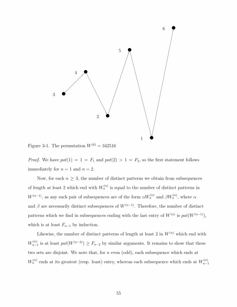
x3
x4
x2
x5
x1
x6
¡¡
¡¡
¡¡A
AAAAAAAAAAA£
£££££££££££££££££CCCCCCCCCCCCCCCCCCCCCCC¥¥¥¥¥¥¥¥¥¥¥¥¥¥¥¥¥¥¥¥¥¥¥¥¥¥¥¥¥
Figure 3-1. The permutation W (6) = 342516
Proof. We have pat(1) = 1 = F1 and pat(2) > 1 = F2, so the first statement follows
immediately for n = 1 and n = 2.
Now, for each n ≥ 3, the number of distinct patterns we obtain from subsequences
of length at least 2 which end with W(n)n is equal to the number of distinct patterns in
W (n−1), as any such pair of subsequences are of the form αW(n)n and βW
(n)n , where α
and β are necessarily distinct subsequences of W (n−1). Therefore, the number of distinct
patterns which we find in subsequences ending with the last entry of W (n) is pat(W (n−1)),
which is at least Fn−1 by induction.
Likewise, the number of distinct patterns of length at least 2 in W (n) which end with
W(n)n−1 is at least pat(W (n−2)) ≥ Fn−2 by similar arguments. It remains to show that these
two sets are disjoint. We note that, for n even (odd), each subsequence which ends at
W(n)n ends at its greatest (resp. least) entry, whereas each subsequence which ends at W
(n)n−1
55
ends at its least (resp. greatest) entry. These are mutually exclusive conditions by our
assumption that each pattern has length at least 2.
We see that indeed we have a lower bound which satisfies the Fibonacci recurrence.
From our previous work, we know that
Fn = Ω
((1 +
√5
2
)n).
The upper bound on the limit supremum is trivial for maxpat, which is necessarily
bounded above by the number of subsequences of an n-permutation, 2n.
Based on empirical evidence, (see sequence A088532 in the On-Line Encyclopedia of
Integer Sequences [32]), it seemed this number may “approach” the trivial upper bound of
2n (the number of all subsets of an n-permutation). In [15] this author constructed a class
of permutations over which it was shown that
limn→∞
maxpat(n)1/n = 2.
However, while confirming our suspicion that the nth root approaches 2, this result
still left open the possibility that maxpat(n)2n → 0 as n → ∞, i.e. the possibility that
maxpat(n) = o(2n). Recently Miller [25] and Albert et al. [14] independently proved with
a refinement of the original class from [15] and more delicate counting techniques that
indeed
limn→∞
maxpat(n)
2n= 1, i.e. maxpat(n) ∼ 2n.
In particular, in [25], Miller showed the wonderfully exact bounds
2n −O(n22n−√2n
)≤ maxpat(n) ≤ 2n −O
(n2n−√2n
).
Definition 17. We generalize the function maxpat by defining, for any pattern σ, the
function
maxpatσ(n) = max pat(π) : π ∈ Sn(σ).
56
Our task is to construct a class of permutations which maximize as much as possible
the function maxpatq(n) for increasing patterns q. First, consider what sort of upper
bounds we can find on maxpatσ(n) for a few simple patterns σ.
Proposition 34. For q = 123, we have the upper bound
maxpatq(n) ≤ t(n) :=n∑
m=0
min
(cm,
(n
m
)),
where cm is the mth Catalan number and counts 123-avoiding permutations of length m.
Furthermore, we have the limit
limn→∞
t(n)1/n = 2.
Proof. For each 0 ≤ m ≤ n, the number of m-patterns in any n-permutation π is at
most the number of subsequences of π of length m, i.e. the number of m-subsets of [n],(
nm
). Similarly, there are at most cm possible 123-avoiding m-patterns. As π itself is
123-avoiding, we know that any pattern contained in π is also 123-avoiding. So, for each
m, the number of m-patterns satisfies both these bounds, and the total number of patterns
is at most the sum of the minima over all m.
The significance of the above limit is that one may hope to pack just as many
patterns into 123-avoiding permutations as in the general case. Furthermore, for any
increasing pattern q = 12 · · · r with r > 3, the same upper bound holds, albeit trivial.
3.2 Pattern Packing in 123-avoiding Permutations
Proposition 34 gives us hope that, even with the 123-avoiding restriction, we
may pack as many patterns as we would like in a permutation of sufficient length.
Experimentation supports such a conjecture. Here we give constructions for q-avoiding
permutations with “many” patterns for increasing patterns q. Our constructions are
modeled on those of [15],[16], [14], and [25] and meet or surpass the original lower bound
57

given for the general case by Wilf,(
1+√
52
)n
. We note that Wilf’s original construction is
132-avoiding, so we already have it established that maxpat132(n) >(
1+√
52
)n
.
We begin with a family of 123-avoiding permutations which show that the limit
infimum of maxpat123(n)1/n is at least 1+√
52
as n →∞.
We define our permutations P (n) inductively. Let P (1) = 1 and P (2) = 12. For each
odd n ≥ 3, let P (n) = nP (n−1), i.e. P (n−1) prepended with n. For each even n ≥ 4, let P (n)
be P (n−1) with n inserted immediately after 1. So, we have
P (1) = 1,
P (2) = 12,
P (3) = 312,
P (4) = 3142,
P (5) = 53142,
P (6) = 531642.
So, each P (n) consists of two decreasing subsequences, and thus avoids 123. The next
proposition gives a lower bound on pat(n) with a proof similar to the proof given for
Proposition 33.
Proposition 35. For all n ≥ 1,
pat(P (n)) ≥ Fn.
Furthermore, we have the bounds
1 +√
5
2≤ lim inf
n→∞maxpat123(n)1/n ≤ lim sup
n→∞maxpat123(n)1/n ≤ 2.
Proof. Our induction hypothesis will be the stronger statement that P (n) contains at least
Fn−1 patterns containing the entry 1. We have that P (1) contains the pattern 1, and P (2)
contains the pattern 12, so the statement of the proposition holds for n = 1 and n = 2.
Assume the statement holds up to and including n ≥ 2. Then, P (n+1) contains a set A
58
of at least pat(P (n)) ≥ Fn−1 patterns which contain the entry (n + 1) and the entry 1.
P (n+1) also contains a set B of at least pat(P (n−1) ≥ Fn−2 patterns which do not contain
the entry (n + 1) but do contain the entries n and 1. We claim that the sets A and B are
disjoint. Indeed, if n + 1 is even (odd), then for each pattern in A the largest entry occurs
after (resp. before) the entry 1, while for each pattern in B the largest entry occurs before
(resp. after) the entry 1. Therefore, we have P (n+1) ≥ Fn−1 + Fn−2 = Fn. The bounds
follow immediately.
3.3 Pattern Packing in q-avoiding Permutations
Next we extend our construction to longer increasing patterns q. Suppose q =
12 · · · (r + 1) is the increasing pattern of length r + 1. We define the permutations Q(n)
inductively. Set Q(1) = 1, Q(2) = 12, . . . , Q(r) = 12 · · · r. For n ≥ r, our permutation
Q(n) consists of r maximal decreasing subsequences. If n + 1 ≡ p (mod r) with 1 ≤ p ≤ r,
we construct Q(n+1) by inserting n + 1 at the beginning of the pth maximal decreasing
subsequence.
Example 36. If q = 12345, i.e. r = 4, we have
Q(5) = 51234,
Q(6) = 516234,
Q(7) = 5162734,
Q(8) = 51627384,
Q(9) = 951627384.
Definition 18. For k ≥ 2, the Fibonacci k-step numbers, denoted F(k)n for n ≥ 0, are
defined by
F (k)n = 0 ∀ n ≤ 0,
F(k)1 = · · · = F
(k)k = 1,
59
and, for all n ≥ k + 1,
F (k)n = F
(k)n−k + F
(k)n−k+1 + · · ·+ F
(k)n−1.
The classical Fibonacci numbers are the special case k = 2.
It is well known that the limit
limn→∞
(F (k)
n
)1/n
is the unique real root greater than 1 of the equation
xk = xk−1 + xk−2 + · · ·+ x + 1.
This root, which we denote by αk, is called the k-anacci constant. We have that αk
increases with k and
limk→∞
αk = 2.
Proposition 37. Let q be the increasing pattern of length r + 1. Then,
pat(Q(n)) ≥ F(r)n−r+2.
Furthermore, we have the bounds
αr ≤ lim infn→∞
maxpatq(n)1/n ≤ lim supn→∞
maxpatq(n)1/n ≤ 2.
Proof. For each 1 ≤ n ≤ r, we only count the pattern Q(n) = 1 · · ·n itself and have
pat(Q(n)) ≥ 1 ≥ F(r)n−r+2.
For n ≥ r + 1, we count the patterns of subsequences which contain the entries 1, 2, . . . , r,
i.e. subsequences which contain the lowest entry of each maximal decreasing subsequence
in Q(n). Fix n ≥ r + 1 and assume by induction that, for all N < n, the number of such
patterns is at least F(r)N−r+2. For 0 ≤ i ≤ r − 1, let Ai be the set of subsequences of Q(n)
which contain the entries 1, 2, . . . , r and whose greatest entry is n− i, and let Bi be the set
of patterns of subsequences in Ai. We claim that the Bi’s are pairwise disjoint. Indeed, for
60

i 6= j, suppose σi ∈ Bi and σj ∈ Bj, where n − i ≡ p (mod r) and n − j ≡ q (mod r),
0 ≤ p, q ≤ r − 1. Then, the greatest entry of σi occurs after p ascents, and the greatest
entry of σj occurs after q ascents.
Also, for each i there is a bijection between the patterns in Bi and the patterns
counted for Q(n−i)−1. So, if we count all patterns in the union of the Bi’s, we have
pat(Q(n)) ≥ pat(Q(n−1)) + · · ·+ pat(Q(n−r)).
As we have the recursion for the Fibonacci r-step numbers, the induction follows.
It may be noted that these classes of permutations resemble the classes used in [15],
[16], [14], and [25], except that whereas in each of these papers the construction consisted
of k rows of k entries each, or a stripped down version of that, the permutations we are
using here have restricted row lengths (number of maximal decreasing subsequences) due
to the q-avoiding restriction.
It was noted that αk → ∞. From this fact we see that as we let r → ∞, our
constructions for increasing patterns of length r + 1 “approach” the constructions for the
general case and the lim infs approach 2.
3.4 Packing Density and Further Directions
Pattern packing is in a weak sense a dual concept to that of pattern avoidance. We
say the duality is only weak as pattern avoidance, when compared to the total number
of permutations, can be understood as the probability that a permutation will have the
property that it avoids the given pattern, whereas the question of pattern packing is
extremal, asking what is the maximum of a certain statistic, the number of patterns
contained in a permutation, over all permutations.
Perhaps the proper dual concept to pattern avoidance question is a question also
posed by Herb Wilf, at the 1992 SIAM Conference on Discrete Mathematics. For a given
pattern σ, how many copies of σ can a permutation contain? The answer depends on the
packing density of the pattern σ.
61
Definition 19. The packing density ρ(σ) of a pattern σ ∈ Sm is defined by
ρ(σ) = limn→∞
g(σ, n)(nm
) ,
where g(σ, n) is the maximum number of copies of σ in any n-permutation.
For more on the work in this area, please see the Ph.D. dissertations of Dan Warren
[38] and Alkes Price [27]. Herb Wilf has recently suggested that the notion of packing
density be examined in the q-avoiding environment.
Why do we raise the issue of these dualities? We saw in the section of pattern
avoidance that in the restricted environments of 123-avoiding permutations, or more
generally q-avoiding permutations, it is more likely that a randomly chosen permutation
avoids some pattern τ , or, critically, the chance of avoiding σ approaches or equals the
chance of avoiding σ′, a statement which is usually false in the general case. So, restricting
to q-avoiding permutations makes our life easier in that work.
However, pattern packing becomes more difficult. Indeed, if we consider all approaches
used to prove pattern packing or superpatterns, they take advantage of a lattice or
checkerboard structure in the class of constructions to bound maxpat. If we restrict the
length of the increasing sequences allowed, we lose this structure. So, the meta-question
is whether we lose our asymptotic limits or simply need more delicate techniques to see
them.
62

CHAPTER 4ASYMPTOTIC NORMALITY AND UNIFORMITY
4.1 Probability Theory
In this paper we only deal with discrete probabilities and their limits. For the sake of
simplicity we avoid the measure theoretic foundations of probability theory and define a
smaller class of random variables, giving associated properties which we will need in this
chapter.
Definition 20. A random variable X is a function from the unit interval [0, 1] to the
real line R. For each r ∈ R, we denote by P (X = r) the Lebesgue measure of the set
ω ∈ [0, 1] : X(ω) = r and call this the probability that X = r. The set of values
X(ω) : ω ∈ [0, 1] we call the range of X. A random variable X is called discrete if its
range is countable or if X has the weaker condition that there is a countable subset B of
the reals with P (X ∈ B) = 1. Finally, a 0-1 random variable or indicator random variable
is a random variable whose range is the set 0, 1.Definition 21. Let X be a random variable with finite range R. The mean or expected
value of X is defined by
E(X) =1
|R|∑r∈R
r.
The variance of X is E((X − E(X))2), which, by the linearity of expectation, is also given
by
Var X = E(X2)− (E(X))2.
The square root of the variance is the standard deviation.
We note that for a 0-1 random variable I, I2 = I, a fact that eases computation
of mean and variance for such variables. Indeed, given a 0-1 random variable I with
P (I = 1) = p, we have E(I) = p and Var I = p− p2.
As we will only be dealing (at least before taking limits) with random variables with
finite range, we will not develop all the measure theory behind these definitions. For this,
the reader is referred to the texts by Halmos [18], Taylor [35], and Chung [13]. For a
63
treatment of discrete probabilities, the reader is referred to the texts by Alon and Spencer
[1] and Charalambides [11].
4.2 Triangular Arrays
Definition 22. Given a random variable Y whose range R is a finite set of integers,
define its probability generating polynomial to be
pY (x) =∑r∈R
P (Y = r)xr.
By a triangular array of nonnegative real numbers (an,k) we mean a sequence of
numbers which are indexed by n = 0, 1, 2, . . ., and k = 0, 1, . . . , m = m(n) for some
function m defined on N, so for each fixed n there is a finite number of terms an,k. The
term triangular array comes to us from the probabilists. When the sequence consists
of non-negative integers, we use the term combinatorial distribution found in [19]. In
combinatorial applications an,k counts objects of size n with some statistic k. For example,
in the next chapter we will study the numbers Sn,k, counting set partitions of an n element
set into k blocks.
Given such a sequence an,k, we set sn = an,1 +an,2 + · · ·+an,m for each n and construct
a new sequence bn,k =an,k
sn, interpreting bn,k as the probability that a randomly selected
n-object has statistic k.
Example 38. A fundamental combinatorial distribution is that of the binomial coefficients(
nk
). It is well known that for each n we have the sum
(n0
)+
(n1
)+ · · · + (
nn
)= 2n. The
generating polynomial
(x + 1)n
2n=
n∑
k=0
(nk
)
2nxk
can be interpreted as the probability generating polynomial for a random variable Xn which
is the sum of n coin flips, i.e. Xn is the sum of n independent 0-1 random variables Yn,k,
k = 1, 2, . . . , n, with
P (Yn,k = 1) =1
2
64
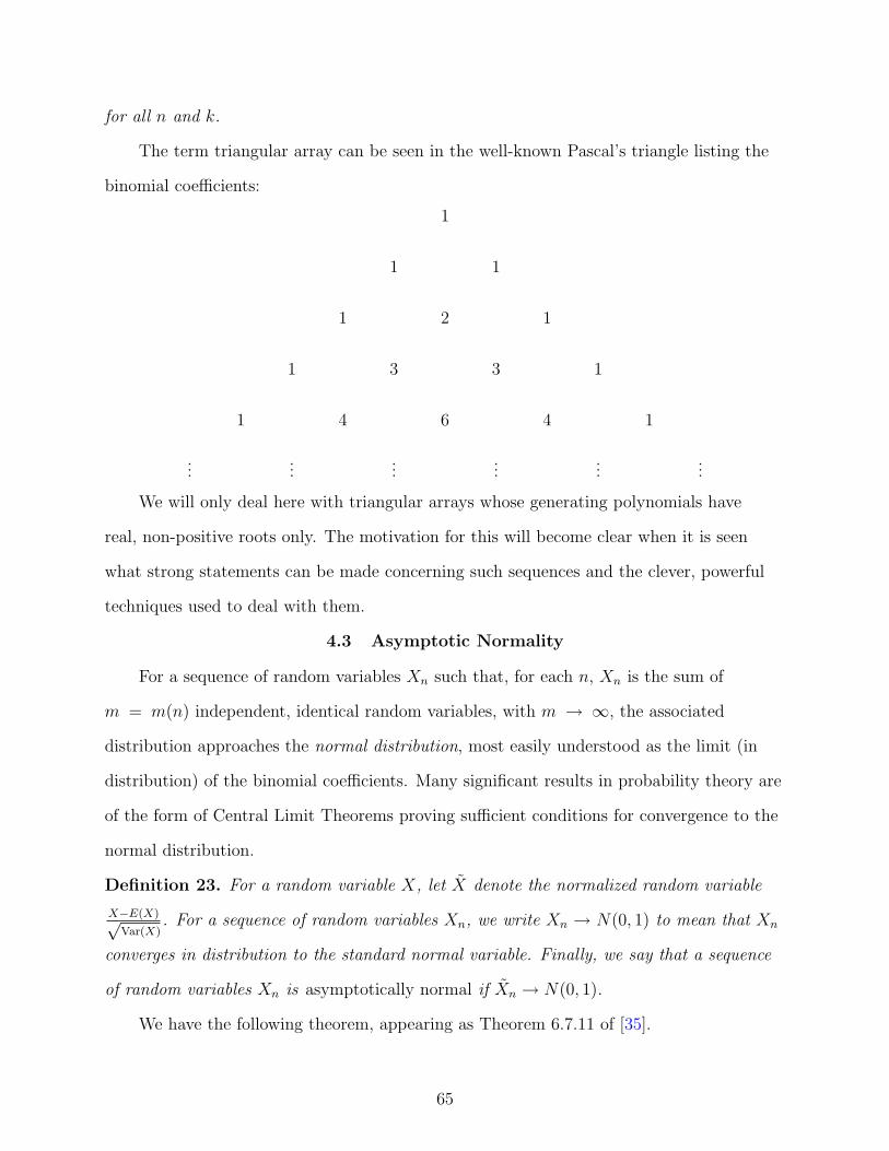
for all n and k.
The term triangular array can be seen in the well-known Pascal’s triangle listing the
binomial coefficients:
1
1 1
1 2 1
1 3 3 1
1 4 6 4 1
......
......
......
We will only deal here with triangular arrays whose generating polynomials have
real, non-positive roots only. The motivation for this will become clear when it is seen
what strong statements can be made concerning such sequences and the clever, powerful
techniques used to deal with them.
4.3 Asymptotic Normality
For a sequence of random variables Xn such that, for each n, Xn is the sum of
m = m(n) independent, identical random variables, with m → ∞, the associated
distribution approaches the normal distribution, most easily understood as the limit (in
distribution) of the binomial coefficients. Many significant results in probability theory are
of the form of Central Limit Theorems proving sufficient conditions for convergence to the
normal distribution.
Definition 23. For a random variable X, let X denote the normalized random variable
X−E(X)√Var(X)
. For a sequence of random variables Xn, we write Xn → N(0, 1) to mean that Xn
converges in distribution to the standard normal variable. Finally, we say that a sequence
of random variables Xn is asymptotically normal if Xn → N(0, 1).
We have the following theorem, appearing as Theorem 6.7.11 of [35].
65

Theorem 39 (Central Limit Theorem for Triangular Arrays). Given a triangular
array of random variables Xn,1, . . . , Xn,m with respective variances σn,1, . . . , xn,m, let
σ2n = σ2
n,1 + · · · + σ2n,m and Xn = Xn,1 + · · · + Xn,m. Then, the distribution
an,k
snconverges
weakly to the unit normal distribution if the Lindeberg condition is satisfied:
∀ε > 0m∑
k=1
1
σ2n
∫
|x|≥σnε
x2Qn,k(dx) → 0 as n →∞,
where, for each k, Qn,k is the cumulative distribution function of Xn,k.
4.4 Asymptotic Uniformity
Another asymptotic property of some combinatorial distributions which provides us
with both qualitative and quantitative understanding of their asymptotic nature is the
concept of asymptotic uniformity. We build up to this with Bona’s definition of balance
([7], [9]).
Definition 24. For each positive integer q, we say that the combinatorial distribution an,k
is q-balanced if for each 0 ≤ r < q, we have the limit
limn→∞
∑k≡r an,k∑
k an,k
=1
q,
where all congruences are modulo q.
So, if an,k counts n-objects with statistic k, q-balance implies that there is eventually
equal probability of a randomly selected n-object to have k-statistic in any one of the
residue classes of q.
Example 40. We give a quick proof that the binomial coefficients are 2-balanced. Evalu-
ating their generating polynomial (x + 1)n at x = −1 gives us the difference of binomial
coefficients for even and odd values of k:
(−1 + 1)n =∑
(−1)k
(n
k
)=
∑
k even
(n
k
)−
∑
k odd
(n
k
).
As (−1 + 1)n = 0n = 0, we have that for all n ≥ 1 the set of evens and the set of odds each
account for exactly half of the total.
66
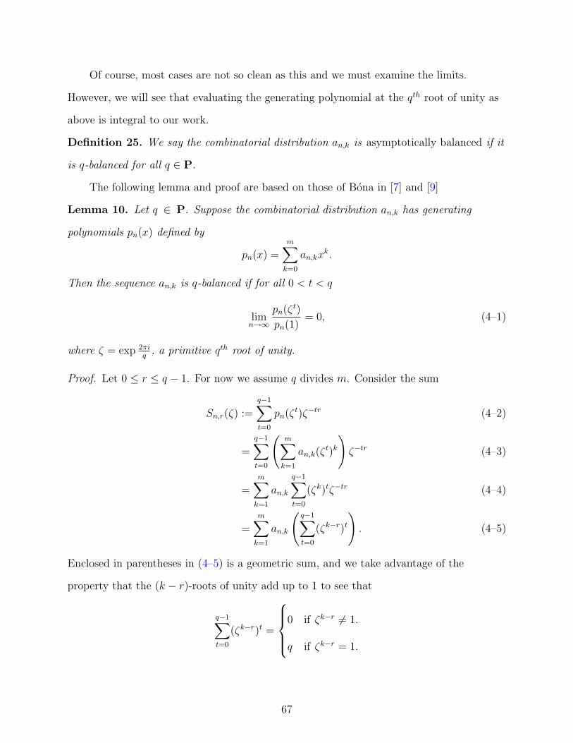
Of course, most cases are not so clean as this and we must examine the limits.
However, we will see that evaluating the generating polynomial at the qth root of unity as
above is integral to our work.
Definition 25. We say the combinatorial distribution an,k is asymptotically balanced if it
is q-balanced for all q ∈ P.
The following lemma and proof are based on those of Bona in [7] and [9]
Lemma 10. Let q ∈ P. Suppose the combinatorial distribution an,k has generating
polynomials pn(x) defined by
pn(x) =m∑
k=0
an,kxk.
Then the sequence an,k is q-balanced if for all 0 < t < q
limn→∞
pn(ζt)
pn(1)= 0, (4–1)
where ζ = exp 2πiq
, a primitive qth root of unity.
Proof. Let 0 ≤ r ≤ q − 1. For now we assume q divides m. Consider the sum
Sn,r(ζ) :=
q−1∑t=0
pn(ζt)ζ−tr (4–2)
=
q−1∑t=0
(m∑
k=1
an,k(ζt)k
)ζ−tr (4–3)
=m∑
k=1
an,k
q−1∑t=0
(ζk)tζ−tr (4–4)
=m∑
k=1
an,k
(q−1∑t=0
(ζk−r)t
). (4–5)
Enclosed in parentheses in (4–5) is a geometric sum, and we take advantage of the
property that the (k − r)-roots of unity add up to 1 to see that
q−1∑t=0
(ζk−r)t =
0 if ζk−r 6= 1.
q if ζk−r = 1.
67

Therefore, we have annihilated all terms in (4–5) for which q does not divide k − r, and
(4–2) reduces to
Sn,r(ζ) = q
m/q∑j=1
an,jq+r, or (4–6)
Sn,r(ζ)
qpn(1)=
∑m/qj=1 an,jq+r
pn(1). (4–7)
We recognize the right hand side of (4–7) as the function from the definition of q-balance.
So, q-balance is equivalent to this expression converging to 1q
for all r, and assuming (4–1)
we can drop our assumption that q divides m, and we have the limit
limn→∞
Sn,r(ζ)
qpn(1)=
1
qlim
n→∞
q−1∑t=0
pn(ζt)
pn(1)ζ−tr
=1
q
q−1∑t=0
ζ−tr limn→∞
pn(ζt)
pn(1)
=1
q(1 + 0 + · · ·+ 0)
=1
q.
4.5 Generating Polynomials with Real, Non-Positive Roots
Throughout this section we will assume that an,k is a triangular array of non-negative
reals whose generating polynomials have real, non-positive roots and set sn = an,0 + an,1 +
· · ·+ an,m. Also, Xn will refer to the random variable defined by
P (Xn = k) =an,k
sn
∀ k ≥ 0,
with probability generating polynomial
pn(x) =m∑
k=0
an,k
sn
xk.
68
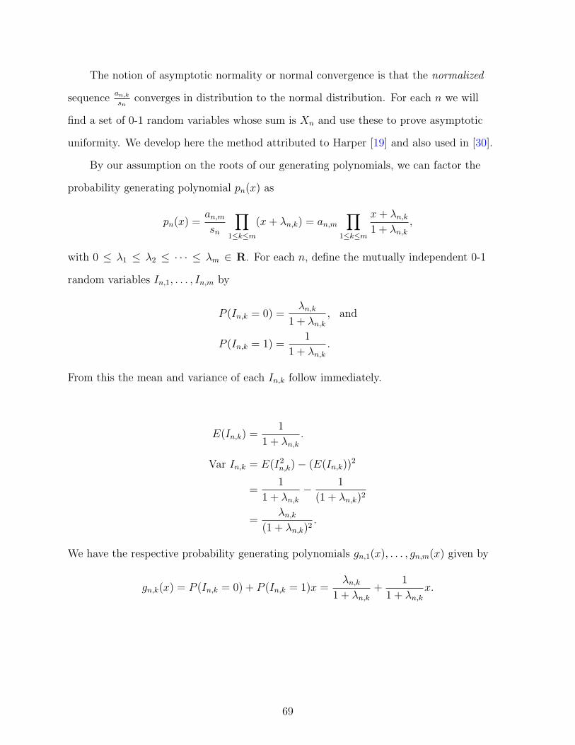
The notion of asymptotic normality or normal convergence is that the normalized
sequencean,k
snconverges in distribution to the normal distribution. For each n we will
find a set of 0-1 random variables whose sum is Xn and use these to prove asymptotic
uniformity. We develop here the method attributed to Harper [19] and also used in [30].
By our assumption on the roots of our generating polynomials, we can factor the
probability generating polynomial pn(x) as
pn(x) =an,m
sn
∏
1≤k≤m
(x + λn,k) = an,m
∏
1≤k≤m
x + λn,k
1 + λn,k
,
with 0 ≤ λ1 ≤ λ2 ≤ · · · ≤ λm ∈ R. For each n, define the mutually independent 0-1
random variables In,1, . . . , In,m by
P (In,k = 0) =λn,k
1 + λn,k
, and
P (In,k = 1) =1
1 + λn,k
.
From this the mean and variance of each In,k follow immediately.
E(In,k) =1
1 + λn,k
.
Var In,k = E(I2n,k)− (E(In,k))
2
=1
1 + λn,k
− 1
(1 + λn,k)2
=λn,k
(1 + λn,k)2.
We have the respective probability generating polynomials gn,1(x), . . . , gn,m(x) given by
gn,k(x) = P (In,k = 0) + P (In,k = 1)x =λn,k
1 + λn,k
+1
1 + λn,k
x.
69
Now we can rewrite each probability generating polynomial pn(x) in terms of the
probability generating polynomials gn,k(x).
pn(x) = an,m
∏
1≤k≤m
x + λn,k
1 + λn,k
= an,m
∏
1≤k≤m
gn,k(x).
We have thus expressed Xn as the sum of the 0-1 random variables In,1, . . . , In,m. We
will be interested in the variance of Xn, which we denote σ2n. We are now in position to
state the following theorem of Bender [3] which follows from Theorem 39:
Theorem 41 (Bender, 73). Let the combinatorial distribution an,k be as above. Then, the
sequence of random variables Xn is asymptotically normal if and only if
σn →∞ as n →∞.
We have the following computation, where 1 ≤ j, k ≤ m for all j, k.
σ2n = E(X2
n)− (E(Xn))2
= E((∑
k
In,k)2)− (
∑
k
E(In,k))2
=∑
k
E(In,k) + 2∑
j<k
E(In,jIn,k)− 2∑
k
(E(In,k))2 −
∑
j<k
E(In,j)E(In,k)
=∑
k
E(In,k)−∑
k
(E(In,k))2
=∑
k
Var In,k
=∑
k
λn,k
(1 + λn,k)2.
With Theorem 41 and keeping the above notation, we have shown the following.
Lemma 11. With real, non-positive zeros, asymptotic normality is equivalent to the
divergence
limn→∞
m∑
k=0
λn,k
(1 + λn,k)2= ∞.
70
4.6 Asymptotic Normality Implies Asymptotic Uniformity
With the results of the above two sections, in particular Lemmas 10 and 11, we can
state the main result of this chapter.
Theorem 42. Let the combinatorial distribution an,k have generating polynomials with
real, non-positive roots only. Then, asymptotic normality implies asymptotic uniformity.
Proof. We retain the notation of Section 4.5. Assuming asymptotic normality, Lemma 11
tells us
m∑
k=1
λn,k
(1 + λn,k)2→∞ as n →∞. (4–8)
By Lemma 10, it suffices to show that this divergence implies
pn(ζr)
pn(1)→ 0 (4–9)
as n →∞ for all q and all 0 < r < q, where ζ = exp 2πiq
. If ζr = −1 is a root of pn(x), then
pn(ζr) = 0, so we can assume here that this is not the case in order to avoid pathologies.
Taking logarithms, (4–9) is equivalent to the condition
m∑
k=1
(log (1 + λn,k)− log |ζr + λn,k|) →∞. (4–10)
By Lemma 12 below, there exists a constant α > 0 which depends only on ζr such that for
all n and k we have
log (1 + λn,k)− log |ζr + λn,k| > αλn,k
(1 + λn,k)2.
Thus,m∑
k=1
(log (1 + λn,k)− log |ζr + λn,k|) > α
m∑
k=1
λn,k
(1 + λn,k)2,
and (4–8) implies (4–10) which is itself equivalent to (4–9).
71

Lemma 12. Let z = eiθ for some 0 < θ < 2π. Then, there exists a constant α = α(z) such
that for all x ≥ 0,
f(x) = log (1 + x)− log |z + x| > αx
(x + 1)2.
Proof. Write f(x) as
f(x) =
∫ x+1
1
dt
t−
∫ |x+z|
1
dt
t=
∫ x+1
|x+z|
dt
t.
The length of the domain of integration is the function d(x) = x + 1− |x + z|, and we have
f(x) >d(x)
x + 1.
So, we are interested in a constant α such that
d(x) > αx
x + 1
for all x ≥ 0. We first show that there is a constant α1 such that d(x) > α1 for all x > 1.
We have the formula |x + z| = (x2 + 2x cos θ + 1)1/2. Therefore, for all x > 1,
d′(x) =d
dx(x + 1− (x2 + 2x cos θ + 1)1/2)
= 1− 2x + 2 cos θ
2(x2 + 2x cos θ + 1)1/2
= 1−(
x2 + 2x cos θ + cos2 θ
x2 + 2x cos θ + 1
)1/2
> 0.
Therefore, d(x) is monotonically increasing for positive x, and for all x > 1 it is greater
than d(1), which we denote by α1.
Next we show there exist constants α2 and δ such that d(x) > α2 for all 0 < x < δ.
We have d′(0) = 1− cos θ, so there exists δ > 0 such that for all 0 < x < δ
d(x) > x1− cos θ
2.
72
Moreover, as 1x+1
< 1, for all 0 < x < δ,
d(x) >1− cos θ
2· x
x + 1,
so we let α2 = 1−cos θ2
. Now we have constants for x ∈ [0, δ) ∪ [1,∞). As [δ, 1] is a compact
set, there exists a constant α3 such that d(x) > α3x
x+1for all x ∈ [δ, 1]. Finally, set α =
min α1, α2, α3.
Example 43. The signless Stirling numbers of the first kind cn,k count n-permutations
with k cycles. For each n, we have the generating polynomial
Cn(x) =n∑
k=1
cn,kxk = x(x + 1) · · · (x + n− 1)
So, for each n, Cn(x) has the roots 0,−1,−2, · · · ,−n + 1. We have the following limit.
limn→∞
n∑j=1
j
(1 + j)2=
∑j≥1
j
1 + j· 1
j
>∑j≥1
1
2· 1
j
→∞
Therefore, by Lemma 11 and Theorem 42, the signless Stirling numbers of the first
kind are asymptotically normal and thus uniform.
73
CHAPTER 5ON THE ROOTS OF THE BELL POLYNOMIALS
5.1 Stirling Numbers of the Second Kind
This chapter is concerned with the generating polynomials for a classic combinatorial
distribution, the Stirling numbers of the second kind. Recalling the notation [n] =
1, 2, . . . , n, we begin with the definition of a fundamental combinatorial object.
Definition 26. For n ∈ P, a set partition of [n], or an n-set partition, is a set of
disjoint, nonempty subsets of [n] called blocks whose union is [n].
Example 44. A set partition of [6] into three blocks is 1, 4, , 2, 3, 5, 6.The natural question posed by an enumerologist is how many such objects are there.
In particular, given non-negative integers n and k, how many set partitions are there of [n]
with k blocks? The answer is the Stirling number of the second kind Sn,k. By convention
we set S0,0 = 1 and Sn,k = 0 for all k > n > 0. The results of this chapter rest primarily on
the following recurrence relation.
Lemma 13. For all n ≥ 0 and 1 ≤ k ≤ n + 1,
Sn+1,k = Sn,k−1 + kSn,k. (5–1)
Proof. Let π be a set partition counted by Sn+1,k. If n + 1 is a block in π, we may
remove it, leaving a set partition of [n] with k − 1 blocks, an object counted by Sn,k−1.
On the other hand, if there are other elements in that block of π which contains n + 1,
we simply remove n + 1 from that block and still have k blocks of n elements, an object
counted by Sn,k. This is clearly an injection and thus shows that the left hand side above
is less than or equal to the right hand side. Now, let γ be a set partition counted by the
right hand side above. If γ has k−1 blocks, we append a block containing only n+1. Else,
we choose one of the k blocks in γ into which we insert n + 1. Again we have an injection,
and the equality holds.
74

Lemma 14. For all n ≥ 1 and 1 ≤ k ≤ n, we have the exact formula
Sn,k =1
k!
k∑i=0
(−1)i
(k
i
)(k − i)n. (5–2)
Furthermore, we have the asymptotic formulae
Sn,k =kn
k!−O((k − 1)n) (5–3)
and
Sn,k ∼ kn
k!. (5–4)
Proof. A set partition of an n-set is constructed by placing the elements into k disjoint
sets. Consider instead the case where there are k labeled boxes and n labeled balls which
we place in the boxes such that no box is empty. Call this an (n, k)-placement and let an,k
be the number of (n, k)-placements. Then, an,k = k! · Sn,k, as there are Sn,k ways to place
the balls into unlabeled boxes, and k! ways to label these boxes. So, it suffices to show that
the summation in (5–2) is an,k.
We apply the method of Inclusion-Exclusion. There are kn ways to distribute the
balls to the boxes, as we have k choices of what to do with each of n balls. However, we
may have overcounted distributions in which a box was left empty, so we subtract the(
k1
)(k − 1)n ways to choose a box to be empty and distribute the balls to the remaining
k − 1 boxes. Now, we have overcounted the distributions in which there are two empty
boxes. Indeed, for some 1 ≤ p < q ≤ k, consider the set of distributions which leave boxes
p and q empty. We counted such a distribution once in the first term, but subtracted
twice in the second term, once for leaving box p empty and once for leaving box q empty.
So, we need to add 1 for each such pair of boxes and each way to leave that pair empty
and distribute the balls to the other boxes,(
k2
)(k − 2)n. This process continues until the
number i of empty boxes reaches zero, and we have the desired sum.
75
For the asymptotics, we write (5–2) as
Sn,k =kn
k!− k(k − 1)n
k!+
k(k − 1)(k − 2)n
2k!− · · · .
As n → ∞, the dominant term is kn
k!. Furthermore, the dominant term of Sn,k − kn
k!is
k(k−1)n
k!, a constant multiple of (k − 1)n, demonstrating (5–3). Finally, as n →∞,
Sn,k
kn
k!
= 1− O((k − 1)n)kn
k!
→ 1.
Lemma 15. For all n ≥ 1 and 1 ≤ k ≤ n, we have the bounds
kn−k ≤ Sn,k ≤ kn
k!(5–5)
and
kn
k!−
dk/2e−1∑i=0
(k
2i + 1
)(k − 2i− 1)n < Sn,k <
kn
k!. (5–6)
Proof. The upper bound, Sn,k ≤ kn
k!, follows trivially from (5–2). By the recurrence (5–1),
for all n > k ≥ 1, we have
Sn,k ≥ kSn−1,k
≥ k2Sn−2,k
≥ · · ·
≥ kn−kSk,k
= kn−k,
as Sk,k = 1 for all k, completing (5–5). The lower bound of (5–6) is the difference of the
dominant term and all odd-indexed, hence negative, terms of (5–2).
76
5.2 Bell Polynomials
For all n ≥ 1, let Bn(x) be the generating polynomial for the Stirling numbers of the
second kind:
Bn(x) =n∑
k=1
Sn,kxk.
These are known as the Bell polynomials.
Example 45. The first few Bell polynomials are as follows.
B0(x) = 1,
B1(x) = x,
B2(x) = x + x2,
B3(x) = x + 3x2 + x3,
B4(x) = x + 7x2 + 6x3 + x4.
Lemma 16. The following recurrence relation on the Bell polynomials holds for all n ≥ 0.
Bn+1(x) = xBn(x) + xB ′n (x). (5–7)
Proof. Applying (5–1) to each term of Bn+1(x), we have
Bn+1(x) =∑
Sn+1,kxk
=∑
(Sn,k−1 + kSn,k)xk
=∑
Sn,k−1xk +
∑kSn,kx
k
= x∑
Sn,k−1xk−1 + x
∑kSn,kx
k−1
= xBn(x) + xB ′n (x).
We have the following well-known result on the roots of the Bell polynomials.
77
Lemma 17. For all n ≥ 1, Bn(x) has n distinct, real, non-positive roots, including zero.
Proof. (Wilf, [40])
The statement holds for B1(x). Assume by induction the statement holds for Bn(x).
Multiplying each term in (5–7) by ex,
exBn+1(x) = x(exBn(x))′.
By Rolle’s theorem, B′n(x) has n − 1 roots, one between each consecutive pair of roots
of Bn(x). Multiplication by x guarantees a root at zero. Since exBn(x) approaches zero
as x → −∞, its derivative has one more root to the left of the leftmost root of Bn(x),
accounting for all n + 1 roots of Bn+1(x).
Thus we can factor each Bell polynomial as
Bn(x) = x(x + λn,2) · · · (x + λn,n), (5–8)
where 0 = λn,1 < λn,2 < · · · < λn,n, and n ≥ 1. In this chapter we explore the roots
λn,k, finding bounds and limits for each fixed k. First, we have a theorem on the Stirling
numbers which builds on the results of the previous chapter but was held aside for the
foregoing definitions and discussion.
Theorem 46. The Stirling numbers of the second kind Sn,k are asymptotically uniform.
Proof. Harper [19] proved that the Stirling numbers of the second kind are asymptotically
normal. The above discussion shows that their generating polynomials have real,
non-positive roots only, so by Theorem 42 in the previous chapter, we achieve the desired
result.
Now, let us consider the roots more closely.
78

Example 47. We solve for the roots of the first few Bell polynomials.
B1(x) = x,
B2(x) = x(x + 1),
B3(x) = x(x +−3 +
√5
2)(x +
−3−√5
2).
For higher n, the algebra becomes unwieldy, as can be readily seen in the other Bell
polynomials given in Example 45.
As our work often deals with sums of products of reciprocals of these roots, for
notational convenience we will write δn,k = 1λn,k
for k = 2, 3, . . . , n, or simply δk = 1λk
if n is
clear from context.
Lemma 18. For all n ≥ 1 and 2 ≤ k ≤ n− 1, we have
Sn,k =∑
λn,i1 · · ·λn,in−k,
where the sum is taken over all (n−k)-tuples i1, i2, . . . , in−k with 2 ≤ i1 < · · · < in−k ≤ n.
Proof. Expanding the factorization in (5–8), an xk term is achieved by choosing x from k
of the terms and λn,i from the remaining n−k terms. The sum of all such products is Sn,k,
the coefficient of xk in Bn(x).
We note that, for all n ≥ 1, we have Sn,n = 1. Lemma 18 could be rewritten to reflect
this by allowing the sum over all (n− n)-tuples to be 1.
Lemma 19. For all n ≥ 2 and all nonempty subsets M ⊆ 2, . . . , n,∏i∈M
λn,i =∏
i∈MC
δn,i,
where MC = 2 ≤ i ≤ n| i 6∈ M is the complement of M .
Proof. We first note that the product of the n− 1 non-zero λn,k’s is Sn,1 = 1, so
n∏
k≥2
λn,k = 1 =n∏
k≥2
δn,k.
79

Thus, for any M ⊆ 2, . . . , n,∏
i∈MC
λn,i
∏i∈M
λn,i = 1, so
∏i∈M
λn,i =
( ∏
i∈MC
λn,i
)−1
∏i∈M
λn,i =∏
i∈MC
δn,i.
Lemma 20. For all n ≥ 1 and 2 ≤ k ≤ n− 1, we have
Sn,k =∑
δn,i1 · · · δn,ik−1, (5–9)
where the sum is taken over all (k−1)-tuples i1, i2, . . . , ik−1 with 2 ≤ i1 < · · · < ik−1 ≤ n.
Proof. Apply Lemma 19 to each (n− k)-tuple in Lemma 18.
For more on Stirling numbers of the second kind and Bell polynomials, particularly
their properties and myriad applications, the reader is referred to the classic by Riordan
[28] as well as the excellent texts by Roman [29] and Wilf [40].
5.3 Bounds on the Roots of the Bell Polynomials
Lemma 21. For all n ≥ 2,
2n−1
n≤ δn,2 < 2n−1.
Proof. By Lemmas 14 and 20 and the nonnegativity of the δn,i’s,
δn,2 ≤n∑
k=2
δn,k = Sn,2 < 2n−1.
As δn,2 is the largest term of the sum, it is at least as large as the mean, so δn,2 > 2n−1−1n−1
.
Finally, this last expression is at least 2n−1
nfor all n ≥ 2.
80
Lemma 22. For all n ≥ 3,
3n−1
2n· 4
9n2≤ δn,3 <
3n−1
2n· n.
Proof. We begin with the upper bound. By Lemmas 14 and 20,
∑2≤i<j≤n
δn,iδn,j = Sn,3 =1
23n−1 −O(2n) <
3n−1
2. (5–10)
In particular,
δn,2δn,3 <3n−1
2.
Applying the inequality δn,2 > 2n−1
nfrom Lemma 21,
δn,3 <3n−1
2δn,2
<n3n−1
2n.
For the lower bound, inequality (5–5) of Lemma 15 provides
Sn,3 > 3n−3.
The next inequality follows from Lemma 20, the fact that the largest of the(
n−12
)terms in
(5–10) is δn,2δn,3, and our upper bound δn,2 < 2n−1.
2n−1δn,3 >3n−3
(n2
) =2 · 3n−3
n(n− 1).
Finally, dividing by 2n−1,
δn,3 >3n−3
2n−1· 2
n(n− 1)
>3n−1
2n· 4
9n2.
81
Theorem 48. For each k ≥ 2, there exist polynomials fk(x) and Fk(x) of degrees 2k−2 and
2k−2 − 1, respectively, such that for all n ≥ k
(k
k − 1
)n1
fk(n)≤ δn,k <
(k
k − 1
)n
Fk(n).
Proof. We induct on k, generalizing the proof of Lemma 22. We proved the statement for
δn,2 and δn,3 in Lemmas 21 and 22, respectively. Let k ≥ 4 and assume by induction that
the statement holds for all δn,j with 2 ≤ j < k. By Lemmas 14 and 20, for all n ≥ k,
∑δn,i1 · · · δn,ik−1
= Sn,k <kn
k!, (5–11)
where the sum is taken over all (k−1)-tuples i1, i2, . . . , ik−1 with 2 ≤ i1 < · · · < ik−1 ≤ n.
By induction we have the following lower bound for each 2 ≤ j < k.
δn,j ≥(
j
j − 1
)n
· 1
fj(n).
which holds for all n ≥ k and where fj(x) is a polynomial of degree 2j−2 for each j
(independent of n). Define the degree 2j−1 − 1 polynomial F (x) = 1k!
f2(x)f3(x) · · · fk−1(x).
Then,
δn,2δn,3 · · · δn,k <kn
k!
δn,k <kn
k!δn,2 · · · δn,k−1
<kn
1
(k − 2)n
(k − 1)n
(k − 3)n
(k − 2)n· · · 2
n
1F (n)
=F (n)kn
(k − 1)n.
For the lower bound, inequality (5–5) of Lemma 15 provides
Sn,k > kn−k.
82

The largest of the(
n−1k−1
)terms in (5–11) is δn,2δn,3 · · · δn,k. By our induction
hypothesis, δn,j obeys the following bound for each 2 ≤ j < k.
δn,j <
(j
j − 1
)n
Fj(n)
for polynomials Fj(x). Altogether,
δn,2δn,3 · · · δn,k >kn−k
(n−1k−1
) ,
δn,k >kn−k
1
(k − 2)n
(k − 1)n
(k − 3)n
(k − 2)n· · · 2
n
1
1
fk(n).
where fk(x) =(
n−1k−1
)F2(x)F3(x) · · ·Fk−1(x).
5.4 Asymptotics of the Roots of the Bell Polynomials
The next two lemmas use our bounds on δn,2 and δn,3 to obtain the asymptotic
equivalences δn,2 ∼ 2n−1 and δn,3 ∼ 3n−1
2n .
Lemma 23. We have the following limit.
limn→∞
δn,2
2n−1= 1.
Proof. The inequality δn,2 < 2n−1 from Lemma 21 implies δn,2
2n−1 < 1 for all n ≥ 2, and it
suffices to show that the terms δn,2
2n−1 are bounded below by a sequence converging to 1. By
Lemmas 14 and 20 we know that Sn,2 = 2n−1 − 1 is the sum of δn,2, δn,3, and n − 3 other
terms, each of which is less than δn,3, so for all n > 3 we have the following inequalities
83

(applying the bound n(
32
)n> δn,3)
δn,2 + nδn,3 > 2n−1,
δn,2 + n2
(3
2
)n
> 2n−1,
δn,2 > 2n−1 − 2n2
(3
2
)n
,
δn,2
2n−1> 1− n2
(3
4
)n
→ 1.
The final limit, in essence 2n2(
34
)n → 0 as n → ∞, holds as 2n2 is a polynomial and(
34
)nis a geometric progression with positive ratio less than one.
Lemma 24. We have the following limit.
limn→∞
δn,32n
3n−1= 1
Proof. Lemma 20 expresses Sn,3 as the sum of all products δiδj. We can split this into two
sums, one sum containing those pairs which include δn,2 and one sum containing all other
pairs,
δn,2
∑i≥3
δn,i +∑
3≤i<j≤n
δn,iδn,j = Sn,3 =3n−1
2−O(2n). (5–12)
We proceed by showing that the second summation above is negligible with respect to
the dominant term 3n−1. Lemma 22 gives us the upper bound δn,3 < n3n−1
2n , and by our
ordering on the δ’s we have δn,j < δn,3 for all j > 3, implying δn,iδn,j <(
n3n−1
2n
)2
for each of
the(
n−22
)pairs i, j with 3 ≤ i < j ≤ n. Thus,
∑3≤i<j≤n
δn,iδn,j <
(n− 2
2
)(n3n−1
2n
)2
<
(9
4
)nn4
2, (5–13)
and∑
3≤i<j≤n
δn,iδn,j = O
((9
4
)n
n4
).
84
Combining (5–12) and (5–13), we have
δn,2
∑i≥3
δn,i = Sn,3 −O
((9
4
)n
n4
)
=3n−1
2−O
((9
4
)n
n4
).
Dividing by our asymptotic approximation of δn,2, δn,2 ∼ 2n−1,
∑i≥3
δn,i =3n−1
2n−O
((9
8
)n
n4
).
By Theorem 48,(
43
)nF4(n) > δn,4 > δn,5 > · · · for the fixed polynomial of degree 3 F4(x),
and (9
8
)n
n4 + (n− 3)
(4
3
)n
F4(n) = O
((4
3
)n
n4
),
so
δn,3 =3n−1
2n−O
((4
3
)n
n4
).
Finally, we divide by 3n−1
2n and take the limit as n →∞.
δn,32n
3n−1= 1−O
((8
9
)n
n4
).
limn→∞
δn,32n
3n−1= lim
n→∞1−O
((8
9
)n
n4
)
= 1.
The following theorem generalizes these results to all k, giving the asymptotic
approximation δn,k ∼ kn−1
(k−1)n for each fixed k.
Theorem 49. For each fixed k, we have the following limit.
limn→∞
δn,k(k − 1)n
kn−1= 1.
Proof. We generalize the proof of the previous lemma to all k ≥ 4. We induct on k, the
cases k = 2 and k = 3 given in the previous two lemmas. The induction hypothesis gives
85

us asymptotic bounds which improve upon those given in the previous section. Indeed, for
all ε > 0 there exists N > 0 such that n > N implies that for all 2 ≤ j < k, we have
δn,j(j − 1)n
jn−1∈ (1− ε, 1 + ε).
We can rewrite equation (5–9) of Lemma 20 as
δn,2δn,3 · · · δn,k−1
∑
j≥k
δn,j +∑
δn,j1 · · · δn,jk−1= Sn,k =
kn
k!−O((k − 1)n), (5–14)
where the second sum is taken over all (k − 1)-tuples 2 ≤ j1 < · · · < jk−1 ≤ n containing
at least two elements which are each at least k. We first show that this summation is
negligible with respect to kn. Let 2 ≤ j1 < · · · < jk−1 ≤ n be such a (k − 1)-tuple. Then,
the product of the greatest k − 3 δn,j’s is bounded above by the product δn,2 · · · δn,k−2, and
the product of the remaining two δn,j’s is bounded above by δ2n,k.
δn,j1 · · · δn,jk−1< δn,2δn,3 · · · δn,k−2δn,kδn,k
< 2n 3n
2n· · · (k − 2)n
(k − 3)nF3(n) · · ·Fk−2(n)
kn
(k − 1)n
kn
(k − 1)nFk(n)Fk(n)
=
(k2(k − 2)
(k − 1)2
)n
G(n),
where G(x) = F3(x) · · ·Fk−2(x)F 2k (x). Set α = k2(k−2)
(k−1)2and note that k − 1 < α < k. The
summation was over a subset of all (k − 1)-tuples, so we overcount the terms by setting
H(x) = G(x)(
nk
)and we can therefore rewrite equation (5–14) as
δn,2δn,3 · · · δn,k−1
∑
j≥k
δn,j =kn
k!−O(αnH(n)). (5–15)
Now, by induction we have
δn,2δn,3 · · · δn,k−1 ∼ 2n−1 3n−1
2n· · · (k − 1)n−1
(k − 2)n
=(k − 1)n−1
(k − 2)!.
86

While the above was an asymptotic approximation, we have the useful information
δn,2δn,3 · · · δn,k−1 = O ((k − 1)n) .
As α > k − 1, this implies
δn,2δn,3 · · · δn,k−1 = O(αn).
Dividing equation (5–15) by (k−1)n−1
(k−2)!,
∑
j≥k
δn,j =kn−1
(k − 1)n−O(βnH(n)), (5–16)
where β = αk−1
= k2(k−2)(k−1)3
. Now it suffices to annihilate all terms on the left hand side
except δn,k. By Theorem 48,
(k + 1
k
)n
Fk+1(n) > δn,k+1 > · · · .
So,
δn,k =kn−1
(k − 1)n−
∑
i≥k+1
δn,i −O(βnH(n))
=kn−1
(k − 1)n−O (βn(H(n) + nFk+1(n))) .
Taking the limit as n →∞, we achieve our desired result.
87
REFERENCES
[1] N. Alon and J. Spencer. The Probabilistic Method. Wiley-Interscience, New York, NY,2000.
[2] R. Arratia. On the Stanley-Wilf conjecture for the number of permutations avoiding agiven pattern. Electronic Journal of Combinatorics, 6(1):N1, 1999.
[3] E. A. Bender. Central and local limit theorems applied to asymptotic enumeration.Journal of Combinatorial Theory, Ser. A, 15:91–111, 1973.
[4] M. Bona. Permutations avoiding certain patterns; the case of length 4 andgeneralizations. Discrete Mathematics, 175:55 – 67, 1997.
[5] M. Bona. Combinatorics of Permutations. Chapman & Hall, Boca Raton, FL, 2004.
[6] M. Bona. The limit of a Stanley-Wilf sequence is not always rational and layeredpatterns beat monotone patterns. Journal of Combinatorial Theory, 110:223–235,2005.
[7] M. Bona. On a balanced property of derangements. Electronic Journal of Combina-torics, 13, 2006.
[8] M. Bona. A Walk Through Combinatorics. World Scientific, River Edge, NJ, 2006.
[9] M. Bona. On a balanced property of compositions. Online Journal of AnalyticCombinatorics, 2, 2007.
[10] M. Bousquet-Melou. Four classes of pattern-avoiding permutations under one roof:Generating trees with two labels. Electronic Journal of Combinatorics, 9(2):R19,2003.
[11] C. A. Charalambides. Combinatorial Methods in Discrete Distributions.Wiley-Interscience, Hoboken, NJ, 2005.
[12] F.R.K. Chung, R.L. Graham, V.E. Hoggatt Jr, and M. Kleiman. The number ofBaxter permutations. Journal of Combinatorial Theory (Series A), 24:382–394, 1978.
[13] K. L. Chung. A Course In Probability Theory. Elsevier, San Diego, CA, 2001.
[14] M. Coleman, M. Albert, I. Leader, and R. Flynn. Permutations containing manypatterns. Annals of Combinatorics, to appear.
[15] Micah Coleman. An answer to a question by Wilf on packing distinct patterns in apermutation. Electron. J. Combin., 11(1):Note 8, 4 pp. (electronic), 2004.
[16] H. Eriksson, K. Eriksson, S. Linusson, and J. Wastlund. Dense packing of patternsin a permutation, Proceedings of the 15th Conference on Formal Power Series andAlgebraic Combinatorics (Melbourne, Australia). http://www.i3s.unice.fr/fpsac/
FPSAC02/articles.html, 2002.
88

89
[17] M. Fekete. Uber die Verteilung der Wurzeln bei gewissen algebraischen gleichungenmit ganzzahligen koeffizienten. Mathematische Zeitschrift, 17:228 – 249, 1923.
[18] P. Halmos. Measure Theory. D. Van Nostrand Co., Berlin, 1956.
[19] L. H. Harper. Stirling behavior is asymptotically normal. Ann. Math. Statist.,38:410–414, 1967.
[20] P. A. Hasto. The packing density of other layered permutations. Electronic Journal ofCombinatorics, 9(2):R1, 2002.
[21] M. Klazar. The Furedi-Hajnal conjecture implies the Stanley-Wilf conjecture. InFormal Power Series and Algebraic Combinatorics, pages 250–255, Berlin, Germany,2000. Springer Verlag.
[22] M. Klazar. Personal communication, 2008.
[23] A. Marcus and G. Tardos. Excluded permutation matrices and the Stanley-Wilfconjecture. Journal of Combinatorial Theory Series A, 107:153–160, July 2004.
[24] D. Marinov and R. Radoicic. Counting 1324-avoiding permutations. ElectronicJournal of Combinatorics, 9(2):R13, 2002.
[25] Alison Miller. Asymptotic bounds for permutations containing many differentpatterns, 2006. preprint.
[26] A. M. Odlyzko. Handbook of Combinatorics, volume 2, chapter AsymptoticEnumeration Methods, pages 1063–1229. Elsevier, Cambridge, MA, 1995.
[27] A. Price. Packing Densities of Layered Patterns. PhD thesis, University ofPennsylvania, 1997.
[28] J. Riordan. An Introduction to Combinatorial Analysis. Wiley, New York, NY, 1980.
[29] S. Roman. The Umbral Calculus. Dover, Mineola, NY, 1984.
[30] A. Rucinski. Random Graphs, chapter 2, Proving Normality in Combinatorics, pages215–231. Wiley Interscience, Cambridge, UK, 1992.
[31] R. Simion and F. W. Schmidt. Restricted permutations. European Journal ofCombinatorics, 6:383 – 406, 1985.
[32] N.J.A. Sloane. The on-line encyclopedia of integer sequences. http://www.research.att.com/~njas/sequences/A088532, 2003.
[33] R. Stanley. Enumerative Combinatorics, Volume 1. Cambridge University Press,Cambridge, UK, 1997.
[34] R. Stanley. Enumerative Combinatorics, Volume 2. Cambridge University Press,Cambridge, UK, 1999.

90
[35] J. Taylor. An Introduction to Measure and Probability. Springer, New York, NY,1997.
[36] V. Vatter. Permutations avoiding two patterns of length three. Electronic Journal ofCombinatorics, 9(2):R6, 2003.
[37] V. Vatter. Small permutation classes. http://arxiv.org/abs/0712.4006, 2007.
[38] D. Warren. Optimizing the Packing Behavior of Layered Permutation Patterns. PhDthesis, University of Florida, 2005.
[39] J. West. Generating trees and forbidden subsequences. Discrete Mathematics, 157(1 -3):363 –374, 1996.
[40] H. Wilf. Generatingfunctionology. A K Peters, Wellesley, MA, 2006.
[41] D. Zeilberger. A loving rendition of the Marcus-Tardos amazing proof of theFuredi-Hajnal conjecture. http://www.math.rutgers.edu/~zeilberg/mamarim/
mamarimPDF/martar.pdf, 2003.

BIOGRAPHICAL SKETCH
A native Florida Cracker, I graduated from Seabreeze High School in 1994 and
entered college as a music major. Realizing my lack of the skill and devotion necessary
for a professional musician, I enlisted in the United States Navy, stationed for four years
in Yokosuka, Japan, where I met my wife Hiroko Shinohara. After my active duty period,
I completed an Associate’s degree at Daytona Beach Community College and joined
my brother and his wife here in Gainesville, entering the world of higher math for the
first time at the University of Florida. As a junior I first met my advisor and fell in love
with Combinatorics. I graduated summa cum laude in 2004 and accepted a fellowship at
UF. I have thoroughly enjoyed my graduate career, even my eight-month sabbatical to
Baghdad, Iraq last year, fully funded by the Naval Reserve. I look forward to a long career
of mathematics research and hope to make some small contribution to the Conversation.
91