permutation tests for linear models in r

Permutation tests for linear models in R

Robert E. Wheeler

2016-07-30

Abstract

An R package which uses permutation tests to obtain p-values for linear models.Standard R linear model functions have been modified to produce p-values obtainedfrom permutation tests instead of from normal theory. These values are advanta-geous when the degrees of freedom for error is small or non-existent, as is the casewith saturated experimental designs, or when the data is drawn from a non-normalpopulation, or when there are apparent outliers. The package also supports ANOVAfor polynomial models such as those used for response surfaces.

1

Contents

1 Introduction 3

2 Examples 5

2.1 lmp() exact . . . . . . . . . . . . . . . . . . . . . . . . . . . . . . . . . . . 6

2.2 lmp() Prob . . . . . . . . . . . . . . . . . . . . . . . . . . . . . . . . . . . . 7

2.3 lmp() SPR . . . . . . . . . . . . . . . . . . . . . . . . . . . . . . . . . . . . 9

2.4 lmp() ANOVA . . . . . . . . . . . . . . . . . . . . . . . . . . . . . . . . . . 9

2.5 aovp() Multistratum analysis . . . . . . . . . . . . . . . . . . . . . . . . . 9

2.6 Saturated designs . . . . . . . . . . . . . . . . . . . . . . . . . . . . . . . . 11

2.7 Overfitting . . . . . . . . . . . . . . . . . . . . . . . . . . . . . . . . . . . . 15

2.8 Polynomial Models . . . . . . . . . . . . . . . . . . . . . . . . . . . . . . . 15

2.9 Multiple responses . . . . . . . . . . . . . . . . . . . . . . . . . . . . . . . 17

2.10 Mixture experiments . . . . . . . . . . . . . . . . . . . . . . . . . . . . . . 17

2.11 ANOVA types . . . . . . . . . . . . . . . . . . . . . . . . . . . . . . . . . . 17

3 Statistical Considerations 24

3.1 Randomized tests and Permutation tests . . . . . . . . . . . . . . . . . . . 24

3.2 Comparing permutation and standard tests . . . . . . . . . . . . . . . . . . 26

3.3 Outliers and non-normal data . . . . . . . . . . . . . . . . . . . . . . . . . 27

4 Technical Details 30

4.1 Permutations . . . . . . . . . . . . . . . . . . . . . . . . . . . . . . . . . . 30

4.2 Linear functionals . . . . . . . . . . . . . . . . . . . . . . . . . . . . . . . . 31

5 Appendix: Derivation of SSb 34

5.1 Non-singular XTX . . . . . . . . . . . . . . . . . . . . . . . . . . . . . . . 34

5.2 Singular XTX . . . . . . . . . . . . . . . . . . . . . . . . . . . . . . . . . . 35

2

1 Introduction

Permutations are fundamental to statistical inference. Consider a simple experiment inwhich three levels of potash are applied to plots and the numbers of lettuce plants thatemerge are tallied, as in Table 1.

Table 1: Lettuce growth experiment

Potash level 1 2 3No. Plants 449 413 326 409 358 291 341 278 312

There seems to be a downward trend in the data with increasing levels of potash:but is it real? The conventional way of deciding this nowadays would be to assume theobservations are normally distributed and drawn from an infinite population of possiblereplications of this experiment. The first assumption cannot be checked, and the secondrequires a good deal of fancy, which doesn’t seem to bother modern researchers verymuch; possibly because they have become used to it. Any assumption that involvesinfinity requires careful thought, since it is quite outside ordinary experience.

In any case, all that is available is this set of 9 observations. If there is a trend, thenone measure of it is the slope of a line fitted through the data. This is given by subtractingthe average of the level 3 observations from the average of the level 1 observations anddividing by 2: it is abut 43. The null hypothesis is that the level of potash does not effectplant growth, which means that the observed value of 43 is due to chance. If it is dueto chance, then there is no connection between the values in Table 1 and the plots fromwhich they come. In other words the first value, 449, could as easily have come from someother plot, and so too for the other values: none of them are tied to the plots shown.That being the case, it is reasonable to ask how frequently chance would create a slope of43 or greater. If 43 is quite common, then it seems unlikely that the trend is real. If onthe other hand, a slope of 43 or larger is rare, then the null hypothesis is suspect.

One can in fact estimate this chance, by permuting the observations in Table 1, andtallying the number of times a slope equal to or greater than 43 is obtained. This valueis a well defined probability, in the same sense that the probability of snake eyes from apair of fair dice is 1/36. It turns out that the probability that a slope will be equal to orgreater than 43 is 0.03912, making it a rare event in most peoples view; and leading tothe conclusion that potash decreases fertility for this planting3.

The rub, of course, is that the conclusion cannot be generalized to the effects of potashon lettuce plants without further assumptions. It is a perfectly correct conclusion for theseparticular plants, and it seems reasonable that it should apply to other plantings, whichcries out for a replication of the experiment. If the same conclusion is reached from anumber of replicated experiments under a variety of conditions, then one would have

1This is a one tailed test, and the corresponding F-test probability is 0.048.2In addition, the randomization is over all 9! = 362880 permutations, instead of over the 1680 combi-

nations obtainable by switching observations only between different levels.3This conclusion is only valid if the hypothesis is posed before the data is observed: the calculations

are meaningless if a salient feature of the data is taken as a hypothesis after the fact.

3

reason to believe it in general. Replication requires care. For example, there may beother factors that influence fertility which should be taken into account, such as the soilgradient or the unequal exposure to sunlight, and repeat experiments might well showsignificant results due to inattention to these factors in the absence of a genuine trend.

Fechner [1860] ran up against such difficulties in establishing a just-noticeable differ-ence for sensory measurement. He presented boxes with various weights to his subjectsand recorded the point at which they were unable to make a judgment. He found it nec-essary to control for many extraneous factors such as the order of presentation and thehand that was used. It took many trials and considerable care to obtain his results.

Peirce and Jastrow [1884] repeated Fechner’s work, but had a wonderful idea: insteadof controlling the many factors, Peirce used a randomizing device which avoided manyof the difficulties that Fechner had encountered. Any factor that might influence theresults of the weighings could be expected to line up with the effect under investigationonly by chance, making the results perhaps more variable, but more nearly correct. Thejust-noticeable difference of Fechner, thus became the point at which the probabilities ofright and wrong judgments were equal.

Moreover, Peirce realized that this device enabled generalizations to be made:

”The truth is that induction is reasoning from a sample taken at random tothe whole lot sampled. A sample is a random one, provided it is drawn by suchmachinery, artificial or physiological, that in the long run any one individualof the whole lot would get taken as often as any other.” [Peirce and Jastrow,1884, p217].

This device of randomization was adopted by Fisher [1935] as a way to generalize theresults from a particular experiment4. Fisher [1925-1952] then invented the idea of a per-mutation test, and provided justification for its use. Because of the computational difficul-ties, approximations such as the chi-squared distribution were used, and over time theseapproximations have replaced permutations as the preferred methodology: see [Fisher,1935, p55]. What is now called the F distribution, in fact, was originally devised as anapproximation for the permutation distribution of the variance ratio – see [Kempthorne,1952, section 7.4]. Computers now make it possible to consider a direct use of permutationtests.

Thus permutation tests applied to suitably randomized experimental units offer a validmethod of induction. The randomization is essential. The use of statistical tests, and inparticular, the use of permutation tests for non-randomized units changes the inferencesthat are possible from the general to the particular. In other words the inferences areproper only for the units involved.

Scheffe [1959] has given a concise definition of permutation tests:

“Permutation tests for a hypothesis exist whenever the joint distribution ofthe observations under the hypothesis has a certain kind of symmetry, namely,

4He must surely have been aware of Peirce’s work, although he did not cite it.

4

when there exists a set of permutations of the observations which leave thedistribution the same (the distributions is invariant under a group of permu-tations).”

In other words, it must be possible under the hypothesis to“exchange”the observations,which occurs for linear models when the hypothesis is the usual null hypothesis and whenthe units have been selected at random from some specific population. If the null is true,then the observed sum of squares, SS, has the same distribution for all permutations ofthe observations, and a tally of the number of values of the SS which exceed that for theoriginal ordering of the observations forms a critical region for the permutation test. Thesize of this region on a proportion scale is the p-value of the permutation test.

There is always the question of choosing the permutation group. For a single variable,one of course permutes all observations. For two variables in a table, one may permute eachrow independently of the row totals, but what about permuting all variables regardless oftheir row? An even more difficult decision is what to do about interactions. [Edgington,1995, p133] argues for a very restricted definition which excludes may effects that areusually of interest to experimenters. The fact is, however, that all estimates are linearfunctions of the observations, as is discussed in Section 4.2, and the coefficients of thesefunctionals depend only on the design. Each coefficient estimate is a function of all theobservations, and thus permutation over observations is meaningful. An exception occurswhen blocks need to be considered, since the linear functionals for such analyses are definedonly over a subset of the observations: R deals with this by projecting the design andthe observations into spaces orthogonal to the blocks, and permutation analyses seems towork well on these projections.

Of course, permutation tests do not assume a particular distribution and are morepowerful in many cases such as for a mixture of distributions or distributions whichdepart substantially from the normal distribution, or when there are outliers. Simulationsillustrating this are shown in Section 3.3

Permutation tests are clearly the method of choice for those vexing cases where thereare no degrees of freedom for error such as for saturated experimental designs, as isillustrated in Section 2.6.

In those cases where the normal theory assumptions are adequately approximated,permutation tests are indistinguishable from the usual F-tests. Section 3.2 shows simu-lations illustrating this. In those cases where the p-values from permutation tests differsubstantially from those for F-tests, a careful examination of the data is usually worth-while.

2 Examples

This section illustrates the several functions in the lmPerm package with a dataset from[Cochran and Cox, 1957, p164].

The dataset is shown in Table(2) is a 3x3 factorial with 9 observations. The y values

5

are numbers of lettuce plants emerging, averaged over 12 plots. The factors are 3 levelsof nitrogen, N, and 3 levels of potash, P. (The Block factor is not part of Cochran andCox’s data set: it will be used for a later illustration.) There are no degrees of freedomfor error.

Cochran and Cox analyzed this data with an external estimate of the residual standarderror. Their analysis indicated that both linear effects were significant.

Table 2: CC164, A 3x3 factorial

y P N Block1 449 1 1 02 413 1 2 23 326 1 3 14 409 2 1 15 358 2 2 06 291 2 3 27 341 3 1 28 278 3 2 19 312 3 3 0

2.1 lmp() exact

The appropriate R function for an analysis of such a data set is lm(), but although itwill estimate the coefficients of the linear model, it will not produce p-values because ofthe lack of an error estimate. The modified function is lmp(), and its output is shown inTable(3). As may be seen, the linear effects are not quite significant at the 5% level5. Thissuggests that Cochran and Cox’s historical value may have been a tad small. Since thereare no residuals the permutation criterion is the unscaled sum of squares, which does notprovide as powerful an analysis as the scaled sum of squares as noted in Section 3.2.

The call for this analysis is

summary(lmp(y~P*N,data=CC164, perm="Exact"))

as indicated at the top of Table(3), which differs only in the perm parameter from thecall that would be made to lm(). The "Exact"6 argument to perm causes all 9!=362,880permutations to be evaluated. The computer response time is not noticeably longer thanfor lm(), which is not the case for larger data sets. In fact 12 or so observations is nearthe limit of my patience at 3 minutes, while 14 is an overnighter. Is it any wonder, withcomputation times like these, that permutations are seldomly used? Before computers,only the simplest permutation calculations were possible, and although things are betternowadays, permutations are still only possible for small data sets. The statistical problemswere resolved by the use of t and F distributions as approximations.

5This is a two tailed test, as are the tests in lmp() and aovp().6The "Exact" argument is redundant here, since it is the default.

6

Table 3: Exact permutation analysis of lettuce data

[1] "Settings: unique SS "

Call:

lmp(formula = y ~ P * N, data = CC164, perm = "Exact")

Residuals:

ALL 9 residuals are 0: no residual degrees of freedom!

Coefficients:

Estimate Pr(Exact)

P.L -60.575 0.0786 .

P.Q 0.408 1.0000

N.L -63.640 0.0643 .

N.Q 4.082 0.8929

P.L:N.L 47.000 0.4656

P.Q:N.L 24.249 0.7075

P.L:N.Q 42.724 0.5052

P.Q:N.Q 13.000 0.8524

---

Signif. codes:

0 '***' 0.001 '**' 0.01 '*' 0.05 '.' 0.1 ' ' 1

Residual standard error: NaN on 0 degrees of freedom

Multiple R-Squared: 1, Adjusted R-squared: NaN

F-statistic: NaN on 8 and 0 DF, p-value: NA

2.2 lmp() Prob

The alternative to evaluating all permutations is to sample from the possible permutationsand to use estimates of p-values. Two methods for doing this are in the present package.The first uses a criterion suggested by Anscombe [1953] which stops the sampling whenthe estimated standard deviation of the p-value falls below some fraction of the estimatedp-value. The second uses the sequential probability ratio of Wald [1947] to decide betweentwo hypotheses about a p-value. There are of course other stopping rules.

Anscombe’s method is controlled by setting perm to "Prob". Thus one has the resultsshown in Table(4).

7

Table 4: Estimated permutation analysis of lettuce data


Call:

lmp(formula = y ~ P * N, data = CC164, perm = "Prob")

Residuals:


Coefficients:

Estimate Iter Pr(Prob)

P.L -60.5755 995 0.0915 .

P.Q 0.4082 51 1.0000

N.L -63.6396 1905 0.0504 .

N.Q 4.0825 51 0.8235

P.L:N.L 47.0000 115 0.4696

P.Q:N.L 24.2487 51 0.7451

P.L:N.Q 42.7239 96 0.5104

P.Q:N.Q 13.0000 51 0.9216

---

Signif. codes:

0 '***' 0.001 '**' 0.01 '*' 0.05 '.' 0.1 ' ' 1




8

Note that Pr(Exact) has changed to Pr(Prob). There is good agreement between thep-values in the two tables, but sampling being what it is, one must not expect certainty.The stopping rule is controlled by a parameter Ca which has a default value of 0.1. That isthe sampling stops when the estimated standard deviation falls below 0.1 of the estimatedp-value.

The Iter column reports the number of iterations (the sample size) required to meetthe stopping rule – the minimum is set to 50. The number of iterations is a very smallfraction of the 9! possible permutations, so small in fact that had previous generationsof statisticians explored this possibility they may well have used permutations more fre-quently. One only has to recall the still unequaled tables produced by Pearson [1933,1956]to realize that extensive computation was no hindrance to their efforts. Indeed groups of“computers” with mechanical calculators were employed in massive routine calculations,such as inverting matrices, up through the 1960’s, when punched card calculators and thefirst computers became available.

2.3 lmp() SPR

Permutation calculations were first used to assess significance and their justification wasas randomization tests Fisher [1935], that is tests which derive their validity from therandomization of the experimental data. They are not well suited to decision theory, andyet decisions theory can be used to assess p-values. If one chooses two hypotheses aboutthe p-values, then one can use a sequential probability ratio test Wald [1947] to decide onwhen to stop the sampling. Table(5) illustrates this. It was obtained by setting the perm

parameter to "SPR". Acceptance of the null hypotheses is shown by 1’s in the Accept

column7.

2.4 lmp() ANOVA

Analysis of variance tables may be produced. For “flat” data, one can use the call

anova(lmp(y~P*N,data=CC164))

with the result shown in Table(6).

2.5 aovp() Multistratum analyses

One may perform a multistratum analyses with a call to aovp() as shown in Table(7).The call was

summary(aovp(y~P*N+Error(Block),CC164)).

7For this illustration, the size of the acceptance region was set to 0.07 instead of the default 0.05, toinsure that a 1 would appear in the Accept column.

9

Table 5: SPR permutation analysis of lettuce data

Call:

lmp(formula = y ~ P * N, data = CC164, perm = "SPR", p0 = 0.07,

p1 = 0.08)

Residuals:


Coefficients:

Estimate Iter Pr(SPR) Accept

P.L -60.57548 4206.00000 0.08250 0

P.Q 0.40825 35.00000 1.00000 0

N.L -63.63961 1681.00000 0.05592 1

N.Q 4.08248 47.00000 0.76596 0

P.L:N.L 47.00000 126.00000 0.33333 0

P.Q:N.L 24.24871 40.00000 0.87500 0

P.L:N.Q 42.72392 78.00000 0.48718 0

P.Q:N.Q 13.00000 35.00000 1.00000 0


Multiple R-Squared: 1,Adjusted R-squared: NaN


Table 6: Anova permutation analysis of lettuce data


Analysis of Variance Table

Response: y

Df R Sum Sq R Mean Sq Pr(Exact)

P 2 11008.7 5504.3 0.2214

N 2 12200.0 6100.0 0.1893

P:N 4 4791.3 1197.8 0.8913

Residuals 0 0.0

10

The Block variable is fictitious, and is introduced just for this illustration. It has nomeaning for the experiment.

The probability for the block stratum is unity, since the test is for a pooling of allcomponents; and in any case there are only two degrees of freedom to permute.

An example with 7 blocks and 6 treatments taken from [Hald, 1952, Table 17.4], maybe used to illustrate this point. An analysis similar to that of 7 is shown in Table 8.

The data seems to show a linear trend in the block means, so an additional variable,L was created as a linear contrast among blocks. The analysis is shown in Table 9, whereit may be seen that there is a statistically significant linear trend.

2.6 Saturated designs

Saturated designs are experimental designs with no degrees of freedom for error, such asthe main effect plans of Plackett and Burman [1946]. They are usually two level designssuch as that shown in Table 10. This particular design and its analysis was discussed byBox [1988] in his critique of Taguchi metods.

Since there are no degrees of freedom for error in such designs, various techniques areused. The usual technique is to leave some of the factors unassigned, and use the pooledestimates from these to estimate error. Simulations show that a sharp bend in the powercurve at 5 degrees of freedom which means that only only needs a few unassigned factorswhen using such designs.

In this case the original author assigned all factors, and chose to pool the smaller effectestimates for an estimate of error. This obviously biased the error estimate and producedseveral spurious effects as pointed out by Box [1988]. He analyzed the data using half-normal plots, and found only two significant effects, ”E” and ”G”. Table 11 shows thelmp() analysis using permutations: it agrees with Box’s analysis, as it should.

11

Table 7: Multistratum Anova permutation analysis of lettuce data


Error: Block

Component 1 :


P:N 2 1970.7 985.33 1

Error: Within

Component 1 :


P 2 11008.7 5504.3 0.64167

N 2 12200.0 6100.0 0.08611 .

P:N 2 2820.7 1410.3 0.81944

---

Signif. codes:

0 '***' 0.001 '**' 0.01 '*' 0.05 '.' 0.1 ' ' 1

Table 8: Anova with a block stratum

> summary(aovp(Y~T+Error(block),Hald17.4))


Error: block

Component 1 :

Df R Sum Sq R Mean Sq

Residuals 6 1483.2 247.2

Error: Within

Component 1 :

Df R Sum Sq R Mean Sq Iter Pr(Prob)

T 4 137.54 34.386 5000 0.0148 *

Residuals 24 236.60 9.858

---

Signif. codes:

0 '***' 0.001 '**' 0.01 '*' 0.05 '.' 0.1 ' ' 1

12

Table 9: Anova with a block stratum and a linear contrast among blocks


Error: block

Component 1 :


L 1 1331.8 1331.79 0.001389 **

Residuals 5 151.4 30.28

---

Signif. codes:

0 '***' 0.001 '**' 0.01 '*' 0.05 '.' 0.1 ' ' 1

Error: Within

Component 1 :


T 4 137.54 34.386 5000 0.0206 *

Residuals 24 236.60 9.858

---

Signif. codes:

0 '***' 0.001 '**' 0.01 '*' 0.05 '.' 0.1 ' ' 1

Table 10: Saturated experimental design with response SN

H D L B J F N A I E M C K G O SN

-1 -1 -1 -1 -1 -1 -1 -1 -1 -1 -1 -1 -1 -1 -1 6.2626

1 -1 1 -1 1 -1 1 -1 1 -1 1 -1 1 -1 1 4.8024

-1 1 1 -1 -1 1 1 -1 -1 1 1 -1 -1 1 1 21.0375

1 1 -1 -1 1 1 -1 -1 1 1 -1 -1 1 1 -1 15.1074

-1 -1 -1 1 1 1 1 -1 -1 -1 -1 1 1 1 1 14.0285

1 -1 1 1 -1 1 -1 -1 1 -1 1 1 -1 1 -1 16.6857

-1 1 1 1 1 -1 -1 -1 -1 1 1 1 1 -1 -1 12.9115

1 1 -1 1 -1 -1 1 -1 1 1 -1 1 -1 -1 1 15.0446

-1 -1 -1 -1 -1 -1 -1 1 1 1 1 1 1 1 1 17.6700

1 -1 1 -1 1 -1 1 1 -1 1 -1 1 -1 1 -1 17.2700

-1 1 1 -1 -1 1 1 1 1 -1 -1 1 1 -1 -1 6.8183

1 1 -1 -1 1 1 -1 1 -1 -1 1 1 -1 -1 1 5.4325

-1 -1 -1 1 1 1 1 1 1 1 1 -1 -1 -1 -1 15.2724

1 -1 1 1 -1 1 -1 1 -1 1 -1 -1 1 -1 1 11.1976

-1 1 1 1 1 -1 -1 1 1 -1 -1 -1 -1 1 1 9.2436

1 1 -1 1 -1 -1 1 1 -1 -1 1 -1 1 1 -1 4.6836

13

Table 11: lmp() analysis of a saturated design.


Call:

lmp(formula = SN ~ ., data = Quinlan)

Residuals:


Coefficients:

Estimate Iter Pr(Prob)

H1 0.8138 77 0.5714

D1 0.8069 51 0.7255

L1 -0.4041 51 0.7059

B1 -0.2917 51 0.8824

J1 0.3332 61 0.6230

F1 -1.1057 170 0.3706

N1 -0.2779 51 0.6667

A1 1.1433 162 0.3827

I1 -0.4888 51 0.7451

E1 -3.5971 5000 0.0050 **

M1 -0.2202 51 0.8824

C1 -1.1409 150 0.4000

K1 1.1893 140 0.4214

G1 -2.3740 1973 0.0487 *

O1 -0.2153 51 0.8235

---

Signif. codes:

0 '***' 0.001 '**' 0.01 '*' 0.05 '.' 0.1 ' ' 1




14

2.7 Overfitting

The response in some “experiments” is almost error free with the fluctuations due only tothe slight variations in the measuring process. An analysis assuming normal errors can bemisleading in such cases. The problem is more common in industrial settings than it is forsociological or biological work. For example some data cited by [Faraway, 2005, page 190]involved measurements on thermoplastic composite strength subjected to several levelsof laser power and tape speed. There were no replicate measurements and the design issaturated if an interaction is included. Table 12 shows a permutation analysis, and it maybe seen from the mean squares that an analysis using F-tests, with the interaction as theerror term, would show both factors to be significant. It is more likely that the data isalmost without error, and the permutation results are the correct ones.

2.8 Polynomial Models

Models for response surfaces use polynomial models such as

E(Y ) = β0 +∑i

βixi +∑ij

βijxixj,

where the {xi} are numerical variables.

R has little support for such models. In particular, it is not possible to perform anANOVA with them: each column of the incidence matrix is treated independently, andthere is no way to pool them into sources, even though the several columns involving thesame variable may represent vectors spanning a space.

lmPerm collects together the appropriate terms in response surface models and pro-duces a correct ANOVA table. For efficient experimental designs, such an analysis willbe meaningful, especially if the variables are centered. Table 13 illustrates this. The firsttwo variables, A and B, are numeric, and the third, C, is a factor.

The function poly.formula() enables a few special functions, such as quad() to beincluded in the formula. The following special functions are available.

> poly.formula(Y~quad(A,B,C))

Y ~ (A + B + C)^2 + I(A^2) + I(B^2) + I(C^2)

> poly.formula(Y~cubic(A,B,C))

Y ~ (A + B + C)^3 + I(A^2) + I(B^2) + I(C^2) + I(A^3) + I(B^3) +

I(C^3)

> poly.formula(Y~cubicS(A,B,C))

15

Table 12: Permutation analysis of tape composite data

> data(composite)

> anova(lmp(strength~laser*tape,composite))



Response: strength


laser 2 224.184 112.092 0.003571 **

tape 2 48.919 24.459 0.557143

laser:tape 4 10.503 2.626 0.990079

Residuals 0 0.000

---

Signif. codes:

0 '***' 0.001 '**' 0.01 '*' 0.05 '.' 0.1 ' ' 1

Table 13: Polynomial model in two variables and a factor

> anova(lmp(poly.formula(Y~quad(A,B)+C),simDesignPartNumeric))

[1] "Settings: unique SS : numeric variables centered"


Response: Y


A 2 2391.02 1195.51 5000 0.0156 *

B 2 459.41 229.70 402 0.2562

A:B 1 77.80 77.80 140 0.4214

C 2 111.67 55.84 103 0.5922

Residuals 6 829.87 138.31

---

Signif. codes:

0 '***' 0.001 '**' 0.01 '*' 0.05 '.' 0.1 ' ' 1

16

Y ~ (A + B + C)^3 + I(A * B * (A - B)) + I(A * C * (A - C)) +

I(B * C * (B - C))

2.9 Multiple responses

The lhs of a formula may reference a matrix in the calling environment, and lm() will pro-duce an analysis for each column as a response variable. aov() will produce a multivariateanalysis. Both lmp() and aovp() produce analyses for each column as the response vari-able. Many datasets contain variables for both the lhs and rhs of the formula, and it isoften convenient to specify the lhs using variables from the argument data. The func-tion multResp() may be used to do this. The dataset Plasma contains three dependentvariables, and Table 14 shows the analysis.

2.10 Mixture experiments

Continuous variables may represent mixtures, as for example, mixtures of components ina paint. In these, the variables are constrained to sum to a constant, usually unity. Anexample of a design for three mixture components is shown in Table (15).

Because of the constraint, ordinary polynomial models will have redundant terms.This may be dealt with by appending non-estimable constraints to the design, or byreformulating polynomial models to account for the constraint. The constraint methodmay be useful in the analysis in those cases where it is desired to interpret the coefficients.Cox [1971] treats this problem. Cox’s results enable models to be build containing bothmixture and non-mixture variables. At the present time neither lmp() nor aovp() supportsuch constraints. For models containing only mixture variables, one may use modelsthat have been given by Scheffe [1958], and elaborated upon by Gorman and Hinman[1962]. The Scheffe models for three variables are shown in Table (16). Note that theconstant term is omitted from these models, which among other things, means that theyare unaffected by block effects.

An analysis of the experiment in Table (15) is shown in Table (17). In this case, asis common for mixture experiments, there is no error in the data, and the analysis isperformed only to create a prediction equation.

2.11 ANOVA types

An ANOVA table summarizes the information about sources in a linear model. Sourcesare of course groups of terms, such as the contrasts associated with a factor. For normaltheory, the likelihood ratio test of the null hypothesis that the source is without effect isobtained as the difference of two residual sums of squares (SS). For example, the differencein the two SS from the following models.

y = µ+ α+ +εy = µ+ α+ β +ε

17

Table 14: Multiple response analysis

> data(Plasma)

> anova(lmp(multResp(Amin,Pct,sinpoly)~.,Plasma))

[1] "Settings: unique SS : numeric variables centered"


Response: Amin


W 1 17332 17332 947 0.09609 .

mTorr 1 47423 47423 3757 0.02608 *

cm 1 393343 393343 5000 < 2e-16 ***

sccm 1 2260 2260 110 0.48182

Residuals 6 27379 4563

---

Signif. codes:

0 '***' 0.001 '**' 0.01 '*' 0.05 '.' 0.1 ' ' 1


Response: Pct


W 1 1.2202 1.2202 420 0.19286

mTorr 1 3.3014 3.3014 1759 0.05401 .

cm 1 3.9105 3.9105 2226 0.04313 *

sccm 1 0.5036 0.5036 316 0.24051

Residuals 6 3.6763 0.6127

---

Signif. codes:

0 '***' 0.001 '**' 0.01 '*' 0.05 '.' 0.1 ' ' 1


Response: sinpoly


W 1 0.027588 0.027588 3380 0.02899 *

mTorr 1 0.019333 0.019333 2259 0.04250 *

cm 1 0.297234 0.297234 5000 < 2e-16 ***

sccm 1 0.000283 0.000283 56 0.64286

Residuals 6 0.017287 0.002881

---

Signif. codes:

0 '***' 0.001 '**' 0.01 '*' 0.05 '.' 0.1 ' ' 1

18

Table 15: ghoctane: An octane-blending experiment

> data(ghoctane)

X1 X2 X3 ON

1 1.000 0.000 0.000 100.8

2 0.000 1.000 0.000 85.2

3 0.000 0.000 1.000 86.0

4 0.500 0.500 0.000 88.8

5 0.500 0.000 0.500 90.3

6 0.000 0.500 0.500 85.5

7 0.333 0.333 0.333 88.3

8 0.150 0.595 0.255 86.6

9 0.300 0.490 0.210 87.6

Table 16: Scheffe modelslinear X1 +X2 +X3

quadratic X1 +X2 +X3 +X1X2 +X1X3 +X2X3

special cubic X1 +X2 +X3 +X1X2 +X1X3 +X2X3 +X1X2X3

cubic X1 +X2 +X3 +X1X2 +X1X2 +X2X3+X1X2(X1 −X2) +X1X3(X1 −X3) +X2X3(X2 −X3)

R modelslinear X1+X1+X3 -1

quadratic (X1+X2+X3)^2 -1

special cubic (X1+X2+X3)^3 -1

cubic poly.formula(Y~cubicS(X1,X2,X3) -1)

If the design is balanced the SS obtained from successively testing all sources add upto the total SS for a model with the constant as its only term. A balanced design is one inwhich the mean centered columns of the incidence matrix for the sources are orthogonalto each other. If the design is not balanced, the SS do not add up. One can of courseapply ANOVA to any design, balanced or not, but it is seldom appropriate to do this forseverely unbalanced data since the statistical tests will not be independent of the othersources in the model. A controversy exists about the ordering of sources in the model;in particular, there are different opinions about whether or not it is appropriate to testa main effect source when its interaction is included in the model. In other words, doesthe difference in SS for the following models provide an appropriate test? Here φ is theinteraction between the other two sources. This problem is discussed in Section 4.2.

y = µ+ α+ +φ+ εy = µ+ α+ β +φ+ ε

In this section we will discuss an unbalanced dataset and analyze it in two ways.

Table 18 shows an unbalanced dataset reproduced in [Scheffe, 1959, p140]. The data

19

Table 17: Octane blending analysis

> anova(lmp(ON~.^3-1,ghoctane))



Response: ON


X1 1 10169.7 10169.7 0.05075 .

X2 1 7422.5 7422.5 0.05144 .

X1:X2 1 12.0 12.0 0.05568 .

X3 1 7410.1 7410.1 0.05145 .

X1:X3 1 6.5 6.5 0.06520 .

X2:X3 1 0.0 0.0 0.76062

X1:X2:X3 1 0.9 0.9 0.09946 .

Residuals 2 0.1 0.0

---

Signif. codes:

0 '***' 0.001 '**' 0.01 '*' 0.05 '.' 0.1 ' ' 1

shows the average weight of litters of rats of four genotypes reared by mothers of fourgenotypes. Is it the litter genotype or the mother genotype that matters most?

20

Table 18: Rat genotype data

MotherLitter A F I JA 61.5 55.0 52.5 42.0A 68.2 42.0 61.8 54.0A 64.0 60.2 49.5 61.0A 65.0 52.7 48.2A 59.7 39.6

F 60.3 50.8 56.5 51.3F 51.7 64.7 59.0 40.5F 49.3 61.7 47.2F 48.0 64.0 53.0F 62.0

I 37.0 56.3 39.7 50.0I 36.3 69.8 46.0 43.8I 68.0 67.0 61.3 54.5I 55.3I 55.7

J 59.0 59.5 45.2 44.8J 57.4 52.8 57.0 51.5J 54.0 56.0 61.4 53.0J 47.0 42.0J 54.0

21

The degree of unbalance in this data is not severe, as may be seen from the following.The columns of the incidence matrix are not orthogonal because of the unequal numberof observations in the cells.

> data(ratGenotype)

> replications(~litter*mother,ratGenotype)

$litter

litter

A B I J

17 15 14 15

$mother

mother

A B I J

16 14 16 15

$`litter:mother`mother

litter A B I J

A 5 3 4 5

B 4 5 4 2

I 3 3 5 3

J 4 3 3 5

An analysis of this data is shown in Table 19. This analysis is sequential and testseach source conditional on the preceding sources in the table. It shows that the rearingis more important than the litter genotype.

A second analysis is shown in Table 20. This analysis makes unique tests on eachsource. That is the SS for each source is conditional on all other sources in the table.It reports essentially the same results, even though the SS are slightly different. (Theparameter seqs is redundant since aovp() will perform a unique analysis by default.)

There may be a problem with unique tests for certain coding of the sources. Let Cbe a contrast matrix for a source, b, and suppose that there is a second factor with threelevels. The columns of the incidence matrix for b will be:

CCC

If the column sums of C are zero, then the cross product of the columns of b and thesecond factor will also be zero, and the two factors are said to be orthogonal; the SS forthe two factors will be independent. This happens for a balanced design. If the design isunbalanced, some of the rows will be missing and the cross product will not be exactly

22

Table 19: Sequential Analysis of rat genotype data

> anova(lmp(wt~litter*mother,ratGenotype,seqs=TRUE))

[1] "Settings: sequential SS "


Response: wt


litter 3 60.16 20.052 165 0.61212

mother 3 775.08 258.360 5000 0.00100 ***

litter:mother 9 824.07 91.564 2826 0.09306 .

Residuals 45 2440.82 54.240

---

Signif. codes:

0 '***' 0.001 '**' 0.01 '*' 0.05 '.' 0.1 ' ' 1

Table 20: Unique Analysis of rat genotype data

> anova(lmp(wt~litter*mother,ratGenotype,seqs=FALSE))



Response: wt


litter 3 27.66 9.219 138 0.9638

mother 3 671.74 223.913 5000 0.0144 *

litter:mother 9 824.07 91.564 1986 0.1208

Residuals 45 2440.82 54.240

---

Signif. codes:

0 '***' 0.001 '**' 0.01 '*' 0.05 '.' 0.1 ' ' 1

23

Table 21: Unique Analysis of rat genotype data using a contrast with non-zero sums.

> anova(lmp(wt~litter*mother,ratGenotype,contrasts=list(mother=contr.treatment(4))))



Response: wt


mother2 12 1599.2 133.26 5000 0.0082 **

Residuals 45 2440.8 54.24

---

Signif. codes:

0 '***' 0.001 '**' 0.01 '*' 0.05 '.' 0.1 ' ' 1

zero. Most of the time the columns sums are near enough to zero, so that this does notmatter. On the other hand, if the column sums of C are quite different from zero, thedeparture from orthogonality can be considerable. Since an interaction is the arithmeticproduct of two factors, this will cause the interaction to be non-orthogonal to the factors,and the unique SS will reflect this because the factors are corrected for the interaction.Table 21 shows the consequence of using a contr.treatment() contrast, whose columnsdo not sum to zero. It should be compared with Table 20. The cross products in theinteraction sum to zero for the mother columns because the litter contrasts sum to zero,but this does not happen for the litter columns. This changes the SS for litter sinceits columns are now dependent on the interaction.

3 Statistical Considerations

3.1 Randomized tests and Permutation tests

It is first of all best to be clear about the distinction between randomization tests andpermutation tests. A randomization test uses permutations to obtain p-values and derivesits legitimacy from the design of the experiment where the “information” is built in byrandomizing the allocation of treatments to trials. A permutation test is simply thepermutation part separated from the logical foundation of a randomization. It can be avalid method of inference but it is not based on randomization assignments of treatmentsto trials.

A leisurely exposition on randomization tests is given by Kempthorne and Doerfler[1969]. In simplest terms, one considers a set of experimental trials involving material(plots, machines, chemical vials, etc.) and treatments (hot-cold, fertilizer, additive, etc.)to be applied to the material. One usually attempts to make the material as homogeneousas possible, but there is a point of diminishing returns in this and so there will alwaysbe some variation in the material. Randomized assignment of treatments to material

24

prevents irregularities in the material from lining up with treatment applications, but thisis not the logic for a randomized test. The logic is as follows. Imagine the experimentat its completion when all the measurements will have been made. Each item will have aresponse value. If the treatment had been the waving of a magic wand over some of thematerial, one would not expect this to have had any effect and the measurements wouldbe exactly the same as if no wand had been waved over them. If, however, on inspectiona “substantial portion” of those items that had been charmed turned out to have moreextreme measurements than the uncharmed ones, then one would be compelled to concedethat something very strange had happened. Either the wand had indeed had an effect,or the results might have occurred because of some unrecognized factor, such as trickery.There is no way to be sure. If, however, the charmed items had been selected at random,these difficulties would disappear, and like it or not, one would have to consider the wandas a possibility and rush out to repeat the experiment.

Judging the“substantial portion” is done by permuting the observations, which obtainsits legitimacy from the randomization that was used to choose the items to be charmed.For if the magic wand had no effect, as we believed to start, then it can have nothing to dowith the measurements that were made and they would be the same no matter which itemswere charmed. It is quite reasonable to ask, then, how the “substantial portion” observedfares when we examine the observations again and pretend that some other possible setof items were charmed. Is our “substantial portion” really large, or is it just largish. Theonly way to find out is to consider all the random allocations that might have been andto calculate the results using the observed data. Thus one permutes the data, calculatesstatistics, and tallies how many randomizations would have produced values as large orlarger than that which was observed. The resulting tally divided by the total number ofpossible permutations is the p-value, a quite legitimate probability, and as good a measureof evidence as can be found. This probability assesses the information that was built intothe experiment during its design by the use of a random mechanism.

On the other hand, a permutation test does not involve randomization of the material.If it is not simply a calculational exercise, it must be judged by other means; one of which isthe selection of material and treatments from some population. If one has two populations,one of witches and one of muggles (about as realistic a pair of populations as many thatare booted about), and if one selects a sample from each and sets them a task, then onemay judge the efficacy of the these populations in performing this task with the aid of apermutation test. The null hypothesis is that witches don’t exist, and those who claim tobe are no more capable of producing charms than are muggles. Say the task is to curdlecream, One might pour bowls of cream for all participants, allow the witches to do theirthing, and at some agreed upon time inspect the bowls for curdling. If upon examiningthe permutation p-value one found it exceeding the 5% level for the witches then the nullwould be rejected; but this p-value would depend for its validity on the random selectionof individuals from the populations which stands in for the randomization of treatmentsused in a randomization test.

25

3.2 Comparing permutation and standard tests

There is no question about the use of permutation and randomization tests for pairedsamples or even for two samples, for surely these were the things used in the earliestdiscussions of permutation and randomization tests. Fisher’s first example (Fisher [1935]used some data of Charles Darwin to illustrate his ideas and the data was in the formof matched pairs. This sort of experiment has been repeated many times and forms astaple in textbooks describing randomized tests. The fact that Darwin probably did notrandomize his data is of no importance (an objection raised by some) because Fishersaid “On the hypothesis that the two series of seeds are random samples from identicalpopulations, and that their sites have been assigned to members of each pair independentlyat random . . .”: [Fisher, 1935, p44]. Fisher was illustrating a method and not performingan analysis with respect to the subject matter.

For more complicated designs, however, it is possible to randomize in different ways,and since the elements that one may exchange in a randomization (permutation) test aredetermined by the randomization it is possible to calculate slightly different p-values indifferent ways. [Edgington, 1995, p133] is adamant about the need to randomize amonglevels of one factor for each set of levels of the other factors: thus for a two-way tablewith factors A and B, he performs a randomization of A for each of the levels of B. Thisvery conservative approach makes the treatment of multi-way tables or blocking factorsdifficult, and pretty nearly eliminates any methodologies for unbalanced designs.

[Manly, 1998, p130] has studied this problem and presents simulations which indicatethat there is little to choose between several methods for main effects when power is con-sidered. In particular, the simulation power values are about the same when Edgington’srules are used as when all observations are randomized. Randomization over all values isof course the easier method. In addition, Manly’s simulations show that randomizationover the residuals is a viable alternative: i.e., for a two-way table with data values xijk,where i and j index the two variables, and k is the replication index, the residuals arerijk = xijk−xi..−x.j. +x..., where dots indicate averaging; thus randomizing the residualsmakes the test conditional on the observed marginal means.

This can be carried further by considering the projection of the observations intosubspaces, as is done with aov() for error subspaces. The aov() function fits the modeldescribed in the Error part of the formula and uses the Q matrix of the qr decompositionto project both the response and the model into orthogonal subspaces in which the otherterms in the formula are fit. Thus if Error describes a block variable, then the formulaterms are fit to data orthogonal to blocks, which amounts to correcting the data withineach block for the block mean. The residuals described in the previous paragraph aredependent since they must sum to zero, and it might be argued that one might wellconsider permuting all but one of them. On the other hand, the orthogonal projection forError describing a block reduces the number of elements by one in each block, and thepermutation for all blocks involves only number of observations minus number of blocks.

In addition, the test statistic makes a difference. For analysis of variance the sum ofsquares, SS, for an effect is a natural choice, but analyses based on this statistic are notas powerful as those based on a sum of squares scaled by the residual sum of squares. The

26

reason is that when effects are present the overall level of the data changes, inflating theSS and making them dependent on this level. The effects of this are illustrated in Table23. The functions lmp() and aovp() use the scaled SS by default.

The functions lmp() and aovp() are modifications of the R functions lm() and aov()that permute the projected response values and output the resulting p-values in place ofnormal theory values. The efficacy of this may be judged by contrasting the two. [Manly,1998, p130] has done this for a number of procedures. A portion of his Table 7.6, filledout with simulations using lmp() and aovp(), is shown in Table 23.

Manly used a 24 observation data set involving two variables in a 4x2 design with 3replicate observations per cell as shown in Table 22. He randomized the response 1000times and applied each of the procedures to the resulting data. He tabulated the numberof times each analysis produced a significant p-value at the 5% level – an estimate of thepower of the test against the alternative hypothesis. Eight alternative hypotheses weregenerated by adding values to the main effects and interactions: these are indicated bythe columns v1,v2,v3 in Table 22. The row labels of Table 23 indicate the v columnsadded to a randomization of the response values; the hi values are obtained by doublingthe v values8. The “S” columns refer to tests based on SS, while the “F” columns refer toSS scaled by the residual SS.

The “F-distribution” columns represent the usual F-test values. The “lmp()” and“aovp()” columns were obtained by using these functions. The “aovp()” analysis hada block variable included to create two strata with perhaps different errors.

As may be seen from this table, there is little to choose between permutation testsand F-tests, even when the permutation tests are based on projections for blocking. Thedifficulties expressed by [Edgington, 1995, p133] do not seem to be of practical importance.The loss of power when unscaled SS are used should be noted.

3.3 Outliers and non-normal data

Linear models assuming normality are fairly insensitive to violation of the assumptionswhen the sample sizes are large. For small samples with few degrees of freedom for error,the size and power of the tests is degraded. Table 24 shows what happens when thedata follows a gamma distribution. The values in this table were obtained from 1000simulations for a 10 observation dataset comprising a single factor at two levels, drawingfive observations from the null distribution with a shape parameter, α, of 0.5, and fiveobservations from several alternatives with shape parameters varying from 0.01 to 1.00.The p-values and powers with respect to a 5% tests, are averaged over the 1000 simulations.The calculation assuming normal errors is clearly less satisfactory than the permutationcalculation.

Unequal variances effect both normal-theory and permutation tests about the same, asmay be seen in Table 25. This table was obtained from 1000 simulations for 10 observationswith powers calculated for a 5% test.

8Manly’s added values were designed to produce effects in each of the three spaces independently, but

27

Table 22: Data used by [Manly, 1998, p126] for power calculaitons

month sex Y v1 v2 v3

1 June Male 13 100 0 0

2 June Male 242 100 0 0

3 June Male 105 100 0 0

4 June Female 182 100 300 0

5 June Female 21 100 300 0

6 June Female 7 100 300 0

7 July Male 8 200 0 0

8 July Male 59 200 0 0

9 July Male 20 200 0 0

10 July Female 24 200 300 0

11 July Female 312 200 300 0

12 July Female 68 200 300 0

13 August Male 515 300 0 0

14 August Male 488 300 0 0

15 August Male 88 300 0 0

16 August Female 460 300 300 300

17 August Female 1223 300 300 300

18 August Female 990 300 300 300

19 September Male 18 0 0 0



22 September Female 140 0 300 300



unfortunately the additions to the interaction space are not orthogonal to the other spaces.

28

Table 23: Power simulations, after [Manly, 1998, p130]. p-values outside the range 3.6%to 6.4%, when true value is 5% are boldfaced.

Unscaled SS Scaled SSlmp() F-distribution lmp() aovp()

Effects S1 S2 S12 F1 F2 F12 F1 F2 F12 F1 F2 F12

1 None 5 7 5 4 5 5 5 5 6 5 5 52 Lo 1 23 4 3 20 5 5 24 6 7 30 5 53 Hi 1 75 1 1 71 4 4 71 5 4 90 6 54 Lo 2 2 57 2 4 56 4 4 58 5 5 74 55 Hi 2 0 100 0 5 100 4 4 100 4 4 100 56 Lo 1,2 16 55 1 21 53 4 20 56 5 33 63 57 Hi 1,2 30 99 0 73 100 3 70 100 4 90 100 68 Lo 1,2,12 10 86 2 51 90 11 29 89 10 42 97 169 Hi 1,2,12 12 100 0 100 100 32 91 100 34 99 100 53

Table 24: Power simulations when the data follows a gamma distribution

αnull αalt F p-val Perm p-val F power Perm power0.5 0.01 0.11 0.03 0.32 0.910.5 0.05 0.17 0.12 0.24 0.630.5 0.10 0.24 0.21 0.18 0.420.5 0.50 0.47 0.51 0.02 0.050.5 1.00 0.37 0.38 0.11 0.16

Table 25: Power simulations when the variances are unequal

µnull σnull µalt σalt F p-val Perm p-val F power Perm power0 1 1.3 1 0.16 0.17 0.42 0.400 1 1.3 4 0.43 0.45 0.12 0.120 1 1.3 8 0.47 0.50 0.08 0.100 1 1.3 16 0.49 0.51 0.07 0.10

29

The exclusion of outliers is a vexed question for which there seems to be no generalanswer. In addition to the problems of choosing criteria for excluding obviously extremevalues, there seem to be situations in which outliers become apparent only in multivariatesituations, [Barnett and Lewis, 1978, p245]. Table 26 shows a power comparison for amixture of normal distributions; the alternative distribution is a mixture of a N(0, 1.3)distribution and with 10% outliers at the values given. The simulations are for 10 obser-vations averaged over 1000 repetitions and the power is for a 5% test. As may be seen,modest outliers have little effect on either method, but larger outliers effect permutationcalculations less than normal theory calculations.

Table 26: Power simulations when there are outliers

µnull µalt µout F p-val Perm p-val F power Perm power0 0 0 0.50 0.50 0.06 0.050 1.3 1 0.18 0.19 0.40 0.380 1.3 2 0.13 0.14 0.50 0.490 1.3 5 0.11 0.11 0.44 0.530 1.3 10 0.16 0.11 0.07 0.53

4 Technical Details

4.1 Permutations

Since permutations are computer intensive calculations, only the fastest algorithms shouldbe used. To the best of my knowledge, the minimal effort general purpose permutationalgorithm is pair exchange; that is successive item pairs are exchanged in a pattern thattraverses all possible permutations. Of course special purpose routines can be writtenthat take advantage of special characteristics of the data: see Baker [1995] for a survey ofmethodologies.

The idea employed here is to observe that if one has a set of permutations of n-1 ele-ments which have been generated with minimal exchanges, then the set of n permutationsobtained by adding a new element at each possible position is also a minimal exchangeset, since each new permutation involves only a pairwise exchange of the new elementwith one of the old elements. The permutation {1,2,3} thus generates the permutations{1,2,3,4}, {1,2,4,3},{1,4,2,3},{4,1,2,3}, each requiring only one pair exchange. A schemefor doing the bookkeeping in this was given by Reingold et al. [1977]. This scheme isembodied in the c code permute.c, and made available in the R package through the Rfunction permute(). A call to permute() produces a list containing pair indexes to beswapped. Using these indexes successively will traverse the possible permutations of a setof elements one pair-swap at a time.

The fact that all possible permutations are traversed by pairwise exchanges enablesthe fast generation of statistics calculated from permutations when the statistics are suchthat they may be updated by calculations involving only the exchanged elements. This is

30

the case when sums of squares are used:all that is involved is the backing out from the sumof squares the contributions from the two pairs, and the addition back in of the switchedcalculations. Since all permutations are generated, the distribution of the statistic is wellcalculated.

Pairwise exchanges are also used when the p-values are estimated by randomly sam-pling from all permutations. Of necessity, the first few permutations generated in thisfashion are similar to the starting one, which raises the question of the representativenessof the sampling. Simulations indicate that starting pairwise permutations from the ob-served values is indeed a bad idea. The convergence to the correct value is very slow. Oneidea is to perform a complete randomization every so often, and indeed this works, butsimply doing a complete randomization at the start seems to be just as good. Simula-tions show that the difference between randomizing every time, and randomizing once atthe start and then using pair exchange, produce equally good estimates of the p-values.Besag and Clifford [1989] have studied this problem and provide justification for the pro-cedure adopted here. The cautious user can control the randomization with the nCycle

parameter.

4.2 Linear functionals

The usual statistics for linear models are derived from linear functionals of the observa-tions; that is if y is the vector of observations, then all of the usual statistics are of theform v′y for some vector v which does not depend on the observations. If Ey = Xβ,and if QR = X, where Q′Q = I, is the qr decomposition of X, then the least squaresestimates of the coefficients are β = R−1Q′y which are linear functionals of y. If theobservations are uncorrelated with unit variances, then the covariance matrix of the leastsquares estimates is (R′R)−1 The squares of the elements of the vector Q′y are the sums ofsquares for the individual coefficients – the squares of linear functionals. If Qb is a matrixof the columns of Q corresponding to a source, then the sum of squares for this sourceis given by summing the elements of (Q′by)2: in other words by summing the squares oflinear functionals of the y’s. This is in fact the methodology used in the LINPACK andLAPACK routines called by lm() and aov() in R.

This methodology produces a sequential breakdown of the sums of squares, as pointedout in the anova.lm() writeup, in which the sum of squares for each source is dependenton sum of squares for the preceding sources. SAS calls this Type I ANOVA. There is noproblem if the sources are orthogonal, since then the sums of squares are unaffected bythe ordering; nor is there a problem when all sources are single degree of freedom sources,as are regression coefficients, since again the source ordering does not affect the sums ofsquares. The difficulty occurs for non-orthogonal (unbalanced) designs where the sourceshave more than one degree of freedom. In this case the order of the sources becomesimportant, since earlier sources constrain later sources.

There is no agreement on how to deal with this problem. One can formulate hypothe-ses about sources individually, which is usually acceptable if the sources are all maineffects but difficulties clearly arise for interactions: should one test main effects when theinteraction is significant? There is a considerable literature on the subject.

31

Part of the problem is due to a data mining mentality in which terms are added andsubtracted to the model in the hope of achieving some goal. The fact that this invalidatesthe statistical tests seems to be overlooked even by those who should know better. Forexample it has been suggested that one ought to routinely omit high level terms unlessthey are significant9.

ANOVA is most appropriately used for designed experiments, and for such experimentsthe model must be supplied in advance of the data collection – there is no room to fiddlewith it after the fact. A computer program should provide significance tests for all sources.It is up to the experimenter to decide whether or not they are relevant.

A significant interaction means that there is a significant contrast in the interactionspace, and almost always implies that the marginal sources are irrelevant. Sometimes thiscontrast is of little interest; for example, it might be due to a single anomalous cell whichcan be explained away. One should look at the interaction means to make a decision. Onthe other hand, a non-significant interaction means that the marginal sources are indeedof interest, and their statistical tests relevant.

The likelihood ratio test under normal theory is a test of two hypotheses, one involvinga source and one not involving the source. The calculations that lead to the test statisticare made by placing the source of interest at the end of the model, which means thatthe source is conditional on the other sources. In common parlance it is “corrected” forall other sources, which seems wrong to many users, especially when main effects are“corrected” for interactions. The fact that single degree of freedom sources (regressioncoefficients) are tested by the same rubric is commonly ignored. This “correction” aspectis however an artifact of the calculation procedure and not the raison d’etre of the test,which rather is a test of a hypothesis.

If one wants to test a main effect in a model with an interaction, and if one wants touse a likelihood ratio test, then the test is the test as stated, and it is equivalent to writingthe model with the source as the last source. That this involves placing the interactionbefore the main effect, is quite irrelevant, since the test is the test is the test. lmPerm

provides a “unique” test for all sources. How they are interpreted is a matter for the user,not the program.

For example Table 28 shows an analysis of Tab1 in Table 27. There is a non-significantinteraction, but a significant main effect. Clearly the main effect is of interest and infor-mative. Had the interaction been significant, however as is shown in Table 29 for Tab2,the main effect might be of less interest, although it clearly indicates that the first rowin the table contains larger values on the average than the second. The statistical testmight be ignored in this case. Part of the controversy has to do with the display of suchinformation: the fear is that it will be misused by occasional statistical users. The fearis real, but twisting oneself into knots to avoid the problem doesn’t seem to make sense.It might be better to abandon the traditional and very useful ANOVA table in favor ofsome display that shows the user Tab2, which makes the relationship very clear.

The technique used by lmPerm may be described by considering the model y = Xβ+ε,

9Although this is impropper, one might implement some sort of regret criteria that would allow fordata snooping.

32

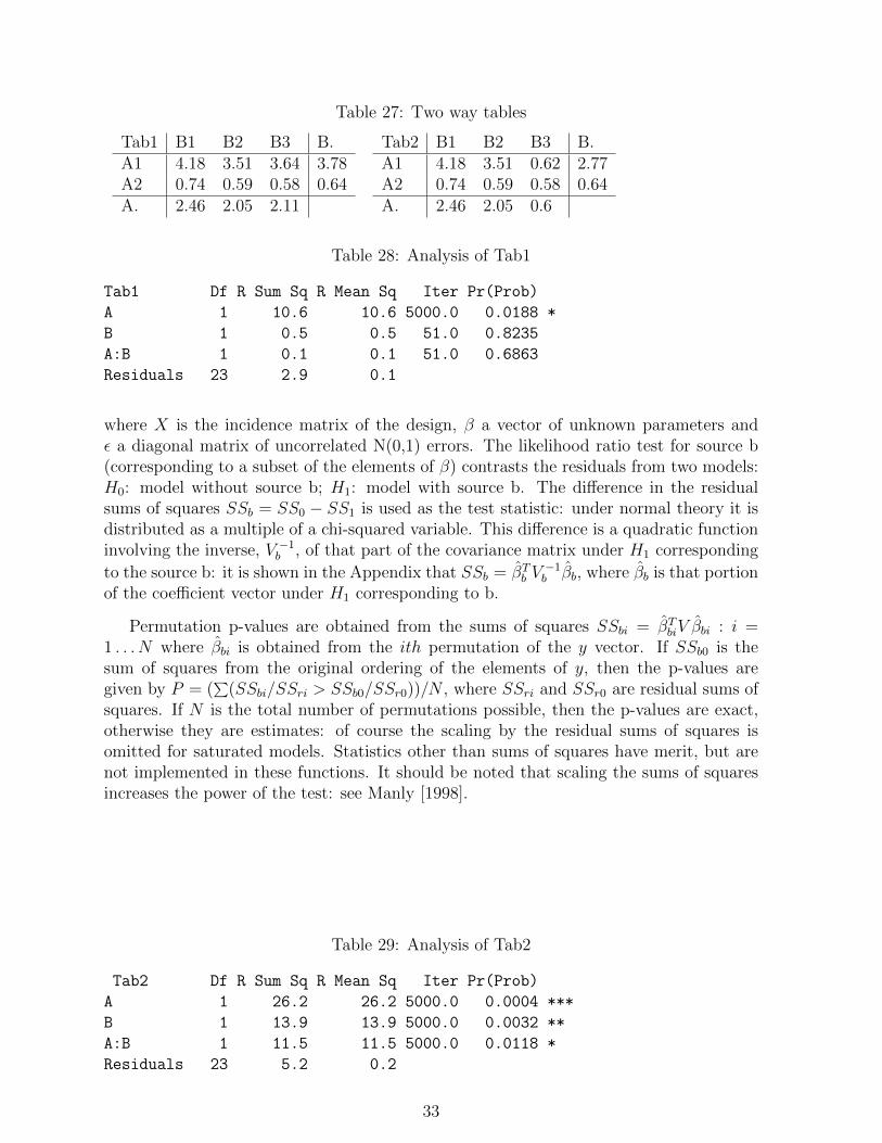
Table 27: Two way tables

Tab1 B1 B2 B3 B.A1 4.18 3.51 3.64 3.78A2 0.74 0.59 0.58 0.64A. 2.46 2.05 2.11

Tab2 B1 B2 B3 B.A1 4.18 3.51 0.62 2.77A2 0.74 0.59 0.58 0.64A. 2.46 2.05 0.6

Table 28: Analysis of Tab1

Tab1 Df R Sum Sq R Mean Sq Iter Pr(Prob)

A 1 10.6 10.6 5000.0 0.0188 *

B 1 0.5 0.5 51.0 0.8235

A:B 1 0.1 0.1 51.0 0.6863

Residuals 23 2.9 0.1

where X is the incidence matrix of the design, β a vector of unknown parameters andε a diagonal matrix of uncorrelated N(0,1) errors. The likelihood ratio test for source b(corresponding to a subset of the elements of β) contrasts the residuals from two models:H0: model without source b; H1: model with source b. The difference in the residualsums of squares SSb = SS0 − SS1 is used as the test statistic: under normal theory it isdistributed as a multiple of a chi-squared variable. This difference is a quadratic functioninvolving the inverse, V −1b , of that part of the covariance matrix under H1 corresponding

to the source b: it is shown in the Appendix that SSb = βTb V−1b βb, where βb is that portion

of the coefficient vector under H1 corresponding to b.

Permutation p-values are obtained from the sums of squares SSbi = βTbiV βbi : i =

1 . . . N where βbi is obtained from the ith permutation of the y vector. If SSb0 is thesum of squares from the original ordering of the elements of y, then the p-values aregiven by P = (

∑(SSbi/SSri > SSb0/SSr0))/N , where SSri and SSr0 are residual sums of

squares. If N is the total number of permutations possible, then the p-values are exact,otherwise they are estimates: of course the scaling by the residual sums of squares isomitted for saturated models. Statistics other than sums of squares have merit, but arenot implemented in these functions. It should be noted that scaling the sums of squaresincreases the power of the test: see Manly [1998].

Table 29: Analysis of Tab2

Tab2 Df R Sum Sq R Mean Sq Iter Pr(Prob)

A 1 26.2 26.2 5000.0 0.0004 ***

B 1 13.9 13.9 5000.0 0.0032 **

A:B 1 11.5 11.5 5000.0 0.0118 *

Residuals 23 5.2 0.2

33

5 Derivation of SSb = βTb V−1βb

5.1 Non-singular XTX

Consider a partitioned incidence matrix X = (X1, X2), and two hypotheses:

H1 : y ∼ N(Xβ1, σ2I)

H2 : y ∼ N(X1β2, σ2I),

with least squares estimates:

y1 = X1βa +X2βband y2 = X1β2.

The two least squares minimums are given by

Lb = (y − y1)T (y − y1) = yTy − yT1 y1La = (y − y2)T (y − y2) = yTy − yT2 y2,

and the sum of squares of interest is

SSb = La − Lb = yT1 y1 − yT2 y2.

We will transform X so that yT1 y1 is the sum of two parts, one of which is yT2 y2, andthe other the desired quadratic function of βb.

Transform X into an orthogonal matrix Z by Z = XT , where

T =

(Ta ∗0 Tb

)T−1 =

(T−1a ∗0 T−1b

),

and the asterisks denote matrices of no interest.

NowI = ZTZ = T TXTXT, (1)

so that

(XTX)−1 = TT T =

(∗ ∗∗ TbT

Tb

)=

(∗ ∗∗ V

),

and σ2V = Cov(βb).

Applying the transformation gives

y1 = Xβ1 = XTT−1β1 = Zγ1 = Z1γa + Z2γb= ya + yb,

34

and because ZT1 Z2 = 0, γ1 and γ2 are estimated independently, so

Z1γa = X1Taγa = X1TaT−1a β2 = X1β2 = y2.

SinceyTa yb = γTa Z

T1 Z2γb = 0,

one has

yT1 y1 = yTa ya + yTb yb.

It follows that

SSb = yT1 y1 − yT2 y2 = yTa ya + yTb yb − yT2 y2 = yTb yb= γTb Z

T2 Z2γb = γTb γb = βT

b (T−1b )TT−1b βb= βT

b (TbTTb )−1βb

= βTb V−1βb.

5.2 Singular XTX

The proof goes thru for singular XTX by choosing Ta, Tb such that instead of equation(1) one has D− = ZTZ, where D is diagonal with elements 0 and 1. Then TDT T is a Ginverse of XTX and TbD2T

Tb = V with V − = (T T

b )−1D−T−1b , hence SSb = βTb V−βb where

βb is the least squares estimate obatined by using TDT T .

References

F.J. Anscombe. Sequential estimation. J. R. Statist. Soc. B, 15:1–29, 1953.

Rose D. Baker. Modern permutation test software. In E.G. Edgington, editor, Random-ization Tests, chapter Appendix. Marcel Decker, 1995.

Vic Barnett and Toby Lewis. Outliers in statistical data. John Wiley and Sons, Inc., NewYork, 1978.

J. Besag and P. Clifford. Generalized monte carlo significance tests. Biometrika, 76(4):633–642, 1989.

G. Box. Signal-to-noise ratios, performance criteria, and transformations. Technometrics,30(1):1–17, 1988.

W.G. Cochran and G. M. Cox. Experimental Designs. John Wiley and Sons,Inc., NewYork, second edition, 1957.

D.R. Cox. A note on polynomial response functions for mixtures. Biometrika, 58(1):155–159, 1971.

35

Eugene S. Edgington. Randomization Tests. Marcel Decker, New York, N.Y., 1995.

Julian Faraway. Linear models with R. Chapman and Hall, New York, 2005.

Gustav Theodor Fechner. Elements of Psychophysics. Holt, Rinehart and Winston, NewYork, N.Y., 1860. Translation of Elemente de Psychophysic, Vol1 by Helmut E. Adler.

R.A. Fisher. Statistical Methods For Reserarch Workers. Hafner, New York, N.Y, 1925-1952.

R.A. Fisher. The Design Of Experiments. Hafner, New York, N.Y, 1935.

J.W. Gorman and J.E. Hinman. Simplex lattice designs for multicomponent systems.Technometrics, 4(4):463–487, 1962.

A. Hald. Statistical theory with engineering applications. Wiley, New York, N.Y., 1952.

O. Kempthorne. The design And Anaysis Of Experiments. Wiley, New York, N.Y, 1952.

Oscar Kempthorne and T.E. Doerfler. The behaviour of some signifcance tests underexperimental randomization. Biometrika, 56(2):231–248, 1969.

Bryan F.J. Manly. Randomization, Bootstrap And MonteCarlo Methods In Biology, Sec-ond. Edition. Chapman & Hall, New York, 1998.

Karl. Pearson. Tables Of The Incomplete Beta-Function. Cambridge Published for theBiometrika Trustees At the University Press, Cambridge, UK, 1933,1956.

Charles Peirce and Joseph Jastrow. On small differences of sensation. Memoirs of theNational Academy of Sciences for 1884, 3:75–83, 1884.

R.L. Plackett and J.P. Burman. The design of optimal multifactorial experiments.Biometrika, 33:305–325, 1946.

E.M. Reingold, Jurg Nievergelt, and Narsingh Deo. Combinatorial Algorithms Theoryand Practice. Prentice Hall, New Jersey, 1977.

H. Scheffe. Experiments with mixtures. Jour. Roy. Statist. Soc (B), 20:344–360, 1958.

H. Scheffe. The Analysis of Variance. Wiley, New York, 1959.

A. Wald. Sequential Analysis. Wiley, New York,N.Y., 1947.

36

permutation tests for linear models in r

Documents