Asset-Pricing Anomalies and Financial Distress

Doron Avramov∗

Department of FinanceRobert H. Smith School of Business

University of Marylanddavramov@rhsmith.umd.edu

Tarun ChordiaDepartment of Finance

Goizueta Business SchoolEmory University

Tarun Chordia@bus.emory.edu

Gergana JostovaDepartment of Finance

School of BusinessGeorge Washington University

jostova@gwu.edu

Alexander PhilipovDepartment of FinanceSchool of Management

George Mason Universityaphilipo@gmu.edu

First draft: February 5, 2007

This Revision: July 16, 2009

∗ We are grateful for financial support from the Q-Group and the FDIC Center for

Financial Research.

Asset-Pricing Anomalies and Financial Distress

Abstract

This paper explores commonalities across asset-pricing anomalies in a unifiedframework. In particular, we assess implications of financial distress for the prof-itability of anomaly-based trading strategies. Strategies based on price momen-tum, earnings momentum, credit risk, dispersion, and idiosyncratic volatility de-rive their profitability from taking short positions in high credit risk firms thatexperience deteriorating credit conditions. Such distressed firms are highly illiq-uid and hard to short sell, which could establish nontrivial hurdles for exploitingthese anomalies in real time. The value effect emerges from taking long positionsin high credit risk firms that survive financial distress and subsequently realizehigh returns. The accruals anomaly is an exception - it is robust amongst highand low credit risk firms as well as during periods of deteriorating, stable, andimproving credit conditions.

Asset pricing theories, such as the capital asset pricing model (CAPM) of Sharpe

(1964) and Lintner (1965), prescribe that riskier assets should command higher expected

returns. Existing theories, however, leave unexplained a host of empirically documented

cross-sectional patterns in average returns, classified as anomalies. Specifically, price mo-

mentum, first documented by Jegadeesh and Titman (1993), reflects the strong abnormal

performance of past winners relative to past losers. Earnings momentum, documented

by Ball and Brown (1968), is a related anomaly1 that describes the outperformance of

firms reporting unexpectedly high earnings relative to those reporting unexpectedly low

earnings. The size and book-to-market effects have been documented, among others,

by Fama and French (1992). In particular, small stocks, as measured by market capi-

talization, have historically outperformed big stocks, and high book-to-market (value)

stocks have outperformed their low book-to-market (growth) counterparts. Sloan (1996)

documents that high accruals stocks underperform low accruals stocks. Dichev (1998),

Avramov, Chordia, Jostova, and Philipov (2009), and Campbell, Hilscher, and Szi-

lagyi (2008) demonstrate a negative correlation between credit risk and average returns.

Diether, Malloy, and Scherbina (2002) show that buying/selling stocks with low/high

dispersion in analysts’ earnings forecasts yields statistically significant and economically

large payoffs. Finally, Ang, Hodrick, Xing, and Zhang (2006) suggest that stocks with

high idiosyncratic volatility realize abnormally low returns.

This paper examines the price momentum, earnings momentum, credit risk, disper-

sion, idiosyncratic volatility, accruals, and value premium anomalies in a unified frame-

work. We explore commonalities across all anomalies and, in particular, assess potential

implications of financial distress, as proxied by credit rating downgrades, for the prof-

itability of anomaly-based trading strategies. It is quite apparent that a downgrade, or

even a concern of financial distress, leads to sharp responses in stock and bond prices. In-

deed, Hand, Holthausen, and Leftwich (1992) and Dichev and Piotroski (2001) show that

bond and stock prices decline considerably following credit rating downgrades. However,

understanding the potential dependence of market anomalies on financial distress is an

unexplored territory. This paper attempts to fill this gap.

Methodologically, our analysis is based on portfolio sorts and cross-sectional regres-

sions, as in Fama and French (2008). Investment payoffs are value-weighted as well as

equally-weighted across stocks. Payoffs based on equally-weighted returns are typically

1See Chordia and Shivakumar (2006).

1

dominated by small stocks which account for a very low fraction of the entire universe

of stocks based on market capitalization, while payoffs based on value-weighted returns

can be dominated by a few big stocks. Our sorting procedure gets around this potential

problem, as investment payoffs are computed separately for micro, small, and big firms,

following the size classification of Fama and French (2008). In addition, we implement

trading strategies within subsamples based on the intersection of best rated, medium

rated, and worst rated firms with micro, small, and large capitalization firms. Credit

ratings, for a total of 4,953 firms and an average of 1,931 firms per month, are obtained

at the monthly frequency from Compustat North America and S&P Credit Ratings.

The analysis, based on both portfolio sorts and cross-sectional regressions, shows that

the profitability of the price momentum, earnings momentum, credit risk, dispersion,

and idiosyncratic volatility anomalies is concentrated in the worst-rated stocks. The

profitability of these anomalies disappears when firms rated BB or below are excluded

from the investment universe. Strikingly, these low-rated firms represent only 6.3% of

the market capitalization of the sample of rated firms. Yet, credit risk is not merely a

proxy for size. In particular, the above anomalies are reasonably robust among all size

groups, including the big low-rated stocks. Moreover, the profitability of these anomalies

is generated almost entirely by the short side of the trade. The value effect also appears

to be related to credit risk. While it is insignificant in the overall sample of firms, it

is significant among low rated stocks, both small and big. The accruals strategy is an

exception, as it is robust across all credit risk groups.

Focusing on financial distress, as proxied by credit rating downgrades, we find that

the profitability of strategies based on price momentum, earnings momentum, credit

risk, dispersion, and idiosyncratic volatility derives exclusively from periods of financial

distress. These strategies provide payoffs that are statistically insignificant and econom-

ically small when periods around credit rating downgrades (from six months before to

six months after a downgrade) are excluded from the sample. None of these strategies

produces significant payoffs during stable or improving credit conditions. Accruals is

again an exception. It is significant during deteriorating, stable, and improving credit

conditions. In contrast, the value anomaly is significant only during stable or improving

credit conditions and comes mostly from long positions in low-rated stocks.

The distinct patterns exhibited by the accruals and value strategies suggest that these

effects are based on different economic fundamentals. The accruals anomaly is based

2

on managerial discretion about the desired gap between net profit and operating cash

flows and this target gap does not seem to depend upon credit conditions. The value

strategy is more profitable in stable credit conditions. The value effect seems to emerge

from long positions in low-rated firms that survive financial distress and realize relatively

high subsequent returns. Thus, while an accruals-based trading strategy is unrelated to

financial distress and a value-based trading strategy bets on low-rated firms surviving

financial distress, the other five anomalies bet on falling prices of low-rated stocks around

periods of financial distress.

A natural questions that emerges is: are market anomalies explained by economy-

wide conditions? Our analysis suggests that the answer is no. Firm rating downgrades

tend to be idiosyncratic events. In particular, we compute a downgrade correlation as

the average pairwise correlation between any two stocks in a particular rating tercile.

Each stock is represented by a binary index taking the value one during a month when

there is a downgrade and zero otherwise. We find that the downgrade correlations are

just too low across the board to indicate that downgrades occur in clusters. In addition,

downgrades do not cluster in up or down markets and they do not cluster over the

business cycle during recessions or expansions.

Finally, we examine whether there are any frictions that prevent these anomalous

returns from being arbitraged away. Indeed, we show that impediments to trading

such as short selling and poor liquidity could establish nontrivial hurdles for exploiting

market anomalies. In particular, low rated stocks are considerably more difficult to short

sell and are substantially more illiquid. Institutional holdings and the number of shares

outstanding for low rated stocks are substantially lower and the Amihud (2002) illiquidity

measure is significantly higher. Low institutional holdings and a low number of shares

outstanding make it difficult to borrow stocks for short selling (see D’Avolio (2002)), and

poor liquidity makes the short transaction quite costly to undertake. Exploiting asset

pricing anomalies would, thus, be relatively difficult in real time because investment

profitability is derived from short positions in low rated stocks that are highly illiquid

and hard to short sell. It should also be noted that investors do not perceive distressed

stocks to be overvalued. The evidence shows that investors are consistently surprised

by the poor performance realized by distressed firms. In particular, analysts covering

distressed firms face large negative earnings surprises and make large negative forecast

revisions.

3

The rest of the paper proceeds as follows. The next section describes the data. Sec-

tion 2 discusses the methodology. Section 3 presents the results and section 4 concludes.

1 Data

The asset-pricing anomalies we study use data on firm return, credit rating, and a variety

of equity characteristics (e.g., the book-to-market ratio, quarterly earnings, and idiosyn-

cratic volatility). The full sample consists of the intersection of all US firms listed on

NYSE, AMEX, and NASDAQ with available monthly returns in CRSP and monthly

Standard & Poor’s Long-Term Domestic Issuer Credit Rating available on Compustat

North America or S&P Credit Ratings (also called Ratings Xpress) on WRDS. Combin-

ing the S&P company rating in Compustat and Rating Xpress provides the maximum

coverage each month over the entire sample period. The total number of rated firms

with available return observations is 4,953 with an average of 1,931 per month. There

are 1,232 (2,196) rated firms in October 1985 (December 2007), when the sample begins

(ends). The maximum number of firms, 2,497, is recorded in April 2000.

The momentum, idiosyncratic volatility, and credit-risk-based trading strategies con-

dition on returns and credit ratings. Hence, the analysis of these anomalies makes use

of the full sample. For the earnings momentum strategy, we extract quarterly earnings

along with their announcement dates from I/B/E/S Detail History Actuals files. The

standardized unexpected earnings (SUE) is computed as the difference between current

quarterly EPS (earnings per share) and EPS reported four quarters ago, divided by the

standard deviation of quarterly EPS changes over the preceding eight quarters. Hence

results for the earnings momentum anomaly are based on the subsample of our rated

firms with SUE data on I/B/E/S, which consists of 3,442 firms with an average of 1,296

firms per month. We also use the I/B/E/S Summary database to obtain dispersion in

analysts’ earning forecasts. As in Diether, Malloy, and Scherbina (2002), dispersion is

calculated as the standard deviation of analyst earnings forecasts for the upcoming fiscal

year end, standardized by the absolute value of the mean (consensus) analyst forecast.

Dispersion observations are excluded if there are less than two analysts covering the

firm. The analysis of the dispersion anomaly is based on a total of 4,074 firms with an

average of 1,429 firms per month. Idiosyncratic volatility is computed as the sum of the

stock’s squared daily returns from CRSP minus the sum of the corresponding squared

4

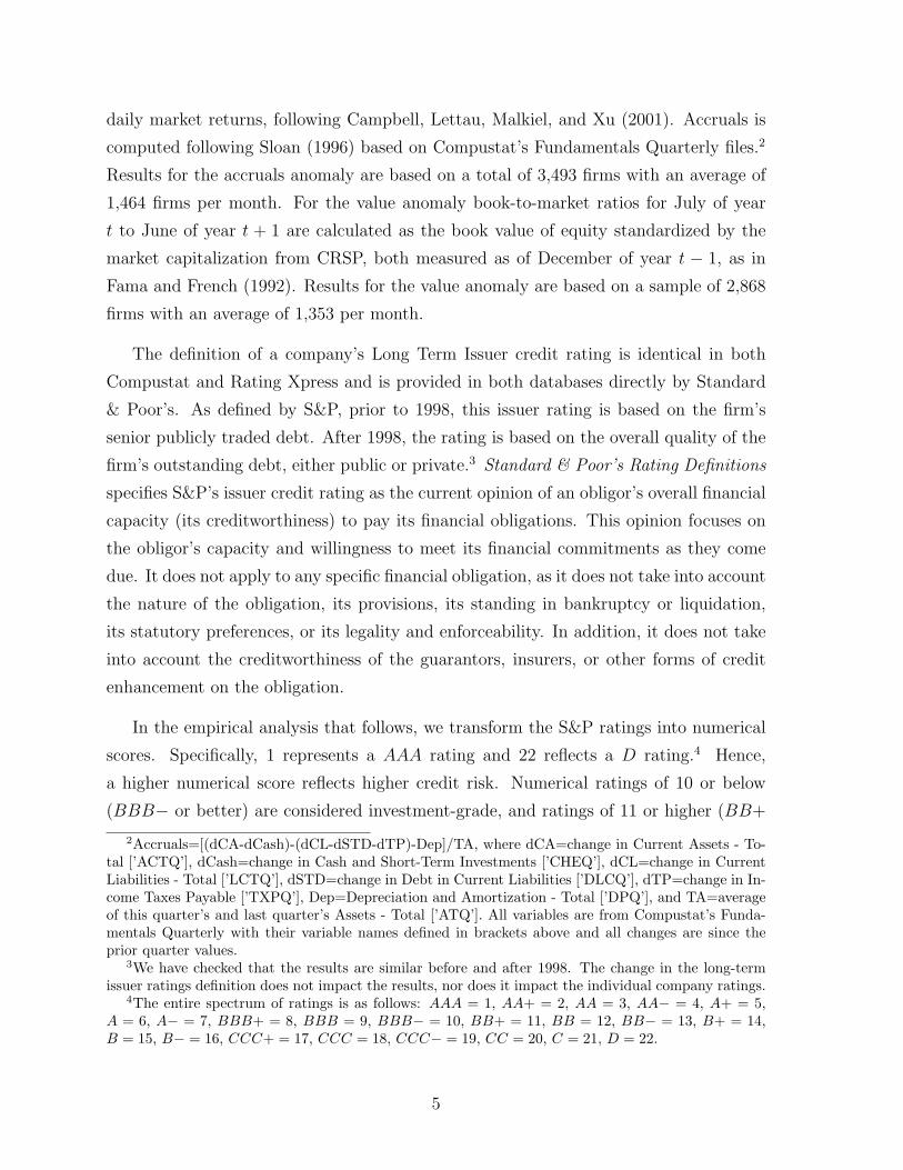
daily market returns, following Campbell, Lettau, Malkiel, and Xu (2001). Accruals is

computed following Sloan (1996) based on Compustat’s Fundamentals Quarterly files.2

Results for the accruals anomaly are based on a total of 3,493 firms with an average of

1,464 firms per month. For the value anomaly book-to-market ratios for July of year

t to June of year t + 1 are calculated as the book value of equity standardized by the

market capitalization from CRSP, both measured as of December of year t − 1, as in

Fama and French (1992). Results for the value anomaly are based on a sample of 2,868

firms with an average of 1,353 per month.

The definition of a company’s Long Term Issuer credit rating is identical in both

Compustat and Rating Xpress and is provided in both databases directly by Standard

& Poor’s. As defined by S&P, prior to 1998, this issuer rating is based on the firm’s

senior publicly traded debt. After 1998, the rating is based on the overall quality of the

firm’s outstanding debt, either public or private.3 Standard & Poor’s Rating Definitions

specifies S&P’s issuer credit rating as the current opinion of an obligor’s overall financial

capacity (its creditworthiness) to pay its financial obligations. This opinion focuses on

the obligor’s capacity and willingness to meet its financial commitments as they come

due. It does not apply to any specific financial obligation, as it does not take into account

the nature of the obligation, its provisions, its standing in bankruptcy or liquidation,

its statutory preferences, or its legality and enforceability. In addition, it does not take

into account the creditworthiness of the guarantors, insurers, or other forms of credit

enhancement on the obligation.

In the empirical analysis that follows, we transform the S&P ratings into numerical

scores. Specifically, 1 represents a AAA rating and 22 reflects a D rating.4 Hence,

a higher numerical score reflects higher credit risk. Numerical ratings of 10 or below

(BBB− or better) are considered investment-grade, and ratings of 11 or higher (BB+

2Accruals=[(dCA-dCash)-(dCL-dSTD-dTP)-Dep]/TA, where dCA=change in Current Assets - To-tal [’ACTQ’], dCash=change in Cash and Short-Term Investments [’CHEQ’], dCL=change in CurrentLiabilities - Total [’LCTQ’], dSTD=change in Debt in Current Liabilities [’DLCQ’], dTP=change in In-come Taxes Payable [’TXPQ’], Dep=Depreciation and Amortization - Total [’DPQ’], and TA=averageof this quarter’s and last quarter’s Assets - Total [’ATQ’]. All variables are from Compustat’s Funda-mentals Quarterly with their variable names defined in brackets above and all changes are since theprior quarter values.

3We have checked that the results are similar before and after 1998. The change in the long-termissuer ratings definition does not impact the results, nor does it impact the individual company ratings.

4The entire spectrum of ratings is as follows: AAA = 1, AA+ = 2, AA = 3, AA− = 4, A+ = 5,A = 6, A− = 7, BBB+ = 8, BBB = 9, BBB− = 10, BB+ = 11, BB = 12, BB− = 13, B+ = 14,B = 15, B− = 16, CCC+ = 17, CCC = 18, CCC− = 19, CC = 20, C = 21, D = 22.

5

or worse) are labeled high-yield or non-investment grade.

Stocks do get delisted from our sample over the holding period. Some stocks delist

due to low prices or bankruptcy while others may delist due to an acquisition or a merger.

Throughout the paper, we use the delisting returns from CRSP whenever a stock gets

delisted.

Summary statistics are reported in Table 1. Each month all stocks rated by S&P are

divided into three portfolios based on their credit rating at time t. For each portfolio, we

compute the cross-sectional median characteristic for month t+1. The reported charac-

teristics represent the time-series averages of the median cross-sectional characteristic.

Not surprisingly, the average firm size (as measured by market capitalization) de-

creases monotonically with deteriorating credit rating. The highest-rated stocks have an

average market capitalization of $3.37 billion, while the lowest-rated stocks have an av-

erage capitalization of $0.33 billion. The book-to-market ratio increases monotonically

with credit risk, from 0.51 in C1 (the lowest rated porfolio) to 0.66 in C3 (the highest

rated portfolio). The average stock price also decreases monotonically with increasing

credit risk from $38.22 for the highest-rated stocks to $12.35 for the lowest-rated stocks.

Notice also that institutions hold fewer shares of low-rated stocks. Institutional holding

(obtained from Thomson’s Financial Database on WRDS) amounts to about 56% of

shares outstanding for high-rated stocks and less than 46% for low-rated stocks.

High-rated firms are considerably more liquid than low-rated firms. The average

monthly dollar trading volume (obtained from CRSP Monthly Stock Files) decreases

from $287 million ($61 million) for the highest-rated NYSE/AMEX (NASDAQ) stocks

to $49 million ($32 million) for the lowest-rated stocks. Moreover, the Amihud (2002)

illiquidity measure is 0.02 (0.23) for NYSE/AMEX (NASDAQ) highest-quality stocks

and 0.48 (0.91) for the lowest-quality stocks.5 This measure is computed as the absolute

price change per dollar of daily trading volume:

ILLIQit =1

Dit

Dit∑t=1

|Ritd|DV OLitd

∗ 107, (1)

where Ritd is the daily return and DV OLitd is the dollar trading volume (both from

5Hasbrouck (2005) compares effective and price-impact measures estimated from daily data to thosefrom high-frequency data and finds that Amihud (2002)’s measure is the most highly correlated withtrade-based measures.

6

CRSP Daily Stock Files) of stock i on day d in month t, and Dit is the number of days

in month t for which data are available for stock i (a minimum of 10 trading days is

required).

We next analyze several variables that proxy for uncertainty about firm’s future fun-

damentals. In particular, the average number of analysts following a firm (obtained from

I/B/E/S) decreases monotonically with credit risk from about 14 for the highest to five

for the lowest-rated stocks. In addition, analyst revisions are negative and much larger

in absolute value for the low-versus-high rated stocks. The standardized unexpected

earnings (SUE) also decreases monotonically from 0.60 for the highest to 0.13 for the

lowest rated stocks. Finally, leverage, computed as the book value of long-term debt

to common equity (’DLTTQ’ to ’CEQQ’ from the Compustat Fundamentals Quarterly

Files), increases monotonically from 0.54 for the highest-rated stocks to 1.36 for the

lowest-rated stocks. Next, market betas increase monotonically from an average of 0.8

for the highest rated stocks to 1.29 for the lowest rated stocks. Finally, the CAPM alpha

decreases from 0.33% for the highest rated stocks to -0.57% for the lowest rated stocks.

Overall, low-rated stocks have smaller market cap, lower price, higher market beta,

lower dollar trading volume, higher illiquidity, higher leverage, lower institutional hold-

ing, and higher uncertainty about their future fundamentals.

2 Methodology

We examine the price momentum, earnings momentum, credit risk, dispersion, idiosyn-

cratic volatility, accruals, and value anomalies. Our analysis is based on both portfolio

sorts and cross-sectional regressions. Focusing on the former, investment payoffs are

value weighted as well as equally weighted across stocks. Payoffs based on equally

weighted returns can be dominated by tiny (microcaps) stocks which account for a very

low fraction of the entire universe of stocks based on market capitalization but a vast

majority of the stocks in the extreme anomaly-sorted portfolios. On the other hand,

value weighted returns can be dominated by a few big stocks. Separately, either case

could result in an unrepresentative picture of the importance of an anomaly.

We run the analysis not only for the entire universe of investable stocks but also for

subsets based on market capitalization and credit ratings. In particular, we implement

7

trading strategies across microcap, small cap, and large cap firms following the classifi-

cations outlined by Fama and French (2008). Microcap firms are those below the 20th

percentile of NYSE stocks, small firms are those between the 20th and 50th percentile of

NYSE stocks, and large firms are those with market capitalizations above the median

NYSE capitalization. The idea here is to examine the pervasiveness of anomalies across

the different market capitalization groups. Similarly, we run the analysis for subsamples

based on credit rating. We examine each anomaly within credit risk terciles: C1 (high-

est quality), C2 (medium quality), and C3 (worst quality). The profitability of each

anomaly is also studied for subsamples based on the interaction of the three size and

three credit rating groups.

Our portfolio formation methodology for all anomalies is consistent with prior liter-

ature. In particular, at the beginning of each month t, we rank all eligible stocks into

quintile portfolios6 on the basis of the strategy-specific conditioning variable (defined

below). P1 (P5) denotes the portfolio containing stocks with the lowest (highest) value

of the conditioning variable based on an J-month formation period. Each strategy buys

one of the extreme quintile portfolios P1 (or P5), sells the opposite extreme quintile

portfolio P5 (or P1), and holds both portfolios for the next K months. Each quintile

portfolio return is calculated as the equally or value weighted average return of the corre-

sponding stocks. When the holding period is longer than a month (K > 1), the monthly

return is based on an equally weighted average of portfolio returns from strategies im-

plemented in the prior month and previous K − 1 months. While the above-described

portfolio formation methodology applies to all strategies studied here, trading strategies

use different conditioning variables and may differ with respect to the formation and

holding periods as well. Below we describe all trading strategies in detail.

The price momentum strategy is constructed as in Jegadeesh and Titman (1993).

Stocks are ranked based on their cumulative return over the formation period (months

t− 6 to t− 1). The momentum strategy buys the winner portfolio (P5), sells the loser

portfolio (P1), and holds both portfolios for six months. We skip a month between the

formation and holding periods (months t + 1 to t + 6) to avoid the potential impact of

short run reversals.

The earnings momentum strategy conditions on the latest standardized unexpected

6Ranking into decile portfolios has delivered similar results. We present results based on quintilesfor consistency with Fama and French (2008).

8

earnings (SUE) reported over the past quarter. The earnings momentum strategy in-

volves buying the portfolio with the highest SUE (P5), selling the portfolio with the

lowest SUE (P1), and holding both portfolios for six months.

The credit risk strategy conditions on prior month credit rating. It involves buying

the best rated quintile portfolio (P1), selling the worst rated quintile portfolio (P5), and

holding both portfolios for one month.

The dispersion-based trading strategy conditions on the prior month standard de-

viation of analyst earnings forecasts for the upcoming fiscal year end, standardized by

the absolute value of the mean (consensus) analyst forecast. The dispersion strategy is

formed by buying P1 (the lowest dispersion portfolio), selling P5 (the highest dispersion

portfolio), and holding both portfolios for one month.

The idiosyncratic volatility strategy conditions on prior month idiosyncratic volatil-

ity, computed as described in the Data section. It involves buying the lowest volatility

quintile (P1), selling the highest volatility quintile (P5), and holding both positions for

one month.

The accruals anomaly conditions on lagged firm level accruals, calculated as explained

in the Data section. There is a four-month lag between formation and holding periods to

ensure that all accounting variables used to form firm level accruals are in the investor’s

information set. The strategy involves buying the lowest accrual portfolio (P1), selling

the highest accrual portfolio (P5), and holding both portfolios for the next 12-month.

The value strategy conditions on the book-to-market ratio, which is calculated as

in Fama and French (1992) and described in the Data section. The strategy involves

buying the highest BM quintile (value stocks: P5), selling the lowest BM quintile (growth

stocks: P1), and holding both portfolios for one month.

3 Results

Table 2 presents monthly returns for the extreme portfolios (P1 and P5) and the differ-

ence between the two (P5-P1 or P1-P5, as noted at the top of each column) for the price

momentum, earnings momentum, credit risk, dispersion, idiosyncratic volatility, accru-

als, and value strategies. Panel A (B) exhibits the size and book-to-market adjusted

9

equally- (value-) weighted portfolio returns. The size and book-to-market adjustment

is made as follows. The monthly return for each stock is measured net of the return

on a matching portfolio formed on the basis of a 5 × 5 independent sort on size and

book-to-market.

Let us first examine investment profitability for all rated firms based on equally

weighted returns. The price momentum strategy yields a winner-minus-loser return of

1.28% per month with the loser (winner) stocks returning -103 (25) basis points. The

earnings momentum strategy yields a 57 basis point monthly return. The credit risk

strategy provides a 91 basis point monthly return. The dispersion strategy returns 60

basis points per month and the idiosyncratic volatility strategy yields 106 basis points per

month. All of the above investment payoffs are economically and statistically significant.

The accruals strategy payoff is a statistically significant 23 basis points per month. The

value strategy delivers the lowest return – a statistically insignificant 19 basis points

per month. Thus, for the overall sample of rated firms, except for the value effect, all

anomaly-based trading strategies are statistically and economically profitable.

Next, we examine trading strategies implemented among microcap, small, and big

firms. The evidence shows that both earnings and price momentum strategies provide

payoffs that monotonically diminish with market capitalization. The payoff to the earn-

ings (price) momentum strategy is 126 (216) basis points per month for microcap stocks.

The corresponding figures are 85 (133) for small stocks and 26 (69) basis points for big

stocks. The P1 portfolio (the short side of the transaction) leads to the large differences

across the size-sorted portfolios. Focusing on earnings (price) momentum, for example,

the P1 portfolio returns -104, -65, and -23 (-162, -114, and -51) basis points per month

for microcap, small, and big stock portfolios, respectively. In contrast, the long side of

the transaction (P5 portfolio) delivers earnings (price) momentum returns of 22, 20, and

3 (53, 18, and 18) basis points per month for the corresponding size groups.

The credit risk and dispersion strategies deliver returns that do not exhibit particular

patterns across the size groups. Both strategies yield the highest (lowest) returns for

the small (microcap) firms. The idiosyncratic volatility strategy payoff decreases mono-

tonically with firm size from 122 basis points per month for microcap stocks to 75 basis

points per month for big stocks. Once again, the return differential around the short

(long) side of the transaction is large (small), amounting to -128, -102, and -78 (-7, 0,

and 3) basis points per month for the microcap, small, and big stocks, respectively. The

10

accruals strategy yields 30 (32) [19] basis points per month for the microcap (small) [big]

firms. The value strategy provides statically significant payoffs of 60 basis points per

month for small stocks only, whereas payoffs based on microcap and big stocks are sta-

tistically insignificant at the 5% level. Interestingly, all anomalies, excluding dispersion,

provides payoffs that are significant at the 10% level, among big rated firms.

Our objective is to examine the impact of credit risk on prominent asset pricing

anomalies. To pursue the analysis, we further partition the sample into high-rated (C1),

medium-rated (C2), and low-rated (C3) stocks.7 The evidence indeed shows that the

impact of credit conditions is quite striking. For instance, the price momentum (accruals)

strategy delivers overall payoffs of 8, 41, and 253 (15, 25, and 28) basis points per month

for the high, medium, and low-rated stocks, respectively. We now analyze, in detail, the

impact of credit ratings on the various asset pricing anomalies.

Amongst the high-rated, C1, firms, no strategy (except for the accruals, which pro-

vides a statistically significant 0.15% monthly return amongst the big stocks) provides

significant payoffs. Amongst the medium-rated, C2, stocks, price momentum is prof-

itable at 52 and 47 basis points per month for small and big firms, respectively. The

earnings momentum strategy is profitable only for small firms, realizing a return of 42

basis points per month. The accruals strategy is profitable for small (33 basis points) and

big (24 basis points) firms. None of the other trading strategies (credit risk, dispersion,

idiosyncratic volatility, or value) displays significant investment payoffs.

Remarkably, all trading strategies are profitable only amongst the low-rated, C3,

stocks. Observe from Table 2 that the highest return (3.05% per month) is earned by

the price momentum strategy upon conditioning on low-rated, microcap stocks. The

next highest investment return (2.35%) per month is also earned by the price momen-

tum strategy but in the intersection of low-rated and small stocks. Even big market cap

stocks having low rating deliver a significant price momentum return of 140 basis points

per month. The earnings momentum and idiosyncratic volatility strategies are prof-

itable across the board for low-rated microcap, small, and big stocks. The idiosyncratic

volatility strategy implemented among low rated stocks yields above 200 basis points

per month for all size groups. The credit risk strategy is profitable for microcap and

small stocks, while the dispersion strategy is profitable only for small low-rated stocks.

7Given our independent sort on firm size and credit rating, there may not be enough stocks belongingto the high-rated, microcap growth (P1) portfolio.

11

The value strategy provides a significant 69 basis point monthly return for small stocks

and 129 basis points for big stocks.

Panel B of Table 2 is the value-weighted counterpart of Panel A. Indeed, the value-

weighted payoffs are often considerably lower, suggesting a role for small firms. For

instance, the overall unconditional return to the price (earnings) momentum strategy

in Panel B is 56 (17) basis points per month, as compared to 128 (57) basis points per

month in Panel A. Nevertheless, investment profitability is typically significant at the

5% or 10% levels amongst big low rated firms. Moreover, investment payoffs generally

increase with worsening credit rating, and all strategies are profitable for small low rated

firms. Only the accruals strategy payoffs are statistically significant across the board for

all credit rating categories. Indeed, the accruals strategy displays a return pattern that

is markedly different from those generated by all other anomalies studied here.

Quite prominent in the results is the overwhelming impact of the short side of the

trading strategies. To illustrate, consider the price momentum strategy. The size-book-

to-market value weighted adjusted return for the winner portfolio is 3 basis points per

month among C1 stocks and 21 basis points among C3 stocks. This represents a return

differential of 18 basis points per month. On the other hand, the return differential across

the loser stocks is 152 [158-6] basis points per month. The short side of the transaction

is clearly the primary source of momentum profitability. Consider now the earnings

momentum strategy. The return differential for the long (short) portfolios across the

low and high-rated stocks is 14 (85) basis points per month. The return differential for

the long (short) portfolios for the credit risk strategy is 28 (134) basis points; for the

dispersion strategy it is 39 (57); for the idiosyncratic volatility strategy it is 17 (196);

for the value strategy it is 33 (73) basis points. Only in the case of the accruals strategy

are the long and short portfolio return differentials similar, 87 versus 80 basis points per

month. This evidence further reinforces the distinctive patterns of the accruals strategy.

Indeed, except for the accruals strategy, the short side of the transaction provides the

bulk of profitability.

Let us summarize the takeaways from Table 2: (i) The profits generated by the

trading strategies typically diminish with improving credit ratings; (ii) Except for the

accruals strategy, the short side of the trade is the primary source of investment prof-

itability; (iii) The accruals strategy is robust across the credit rating sorted portfolios;

(iv) Most trading strategies (all but value and dispersion) are remarkably robust across

12

the size-sorted portfolios; (v) Focusing on value-weighted portfolios, trading strategies

(excluding accruals) are especially profitable among small stocks, though the intersec-

tion of big market cap low credit rating stocks still gives rise to significant investment

payoffs. Indeed, the overall evidence suggests that credit risk plays an important role in

explaining the source of market anomalies.

To further pinpoint the segment of firms driving investment profitability, we doc-

ument in Table 3 the equally-weighted size and book-to-market adjusted returns for

various credit rating subsamples as we sequentially exclude the worst-rated stocks. We

display investment payoffs for all stocks belonging to each of the rating categories as

well as sub groups of microcap, small, and big stocks.

The starting point pertains to all rating categories (AAA-D). The results here are

identical to those exhibited in Panel A of Table 2. Note from the last two columns of

the table that whereas microcap stocks consist of 17.81% of the total number of stocks,

they account only for 0.43% of the market capitalization; small stocks comprise 27.07%

of the total number of stocks and 2.97% of the total market capitalization; big firms

comprise 55.12% of the total number of stocks and an overwhelming 96.59% of the total

market capitalization. Fama and French (2008) report that the microcap stocks account

for 3.07%, small stocks account for 6.45%, and big stocks account for 90.48% of the total

market capitalization. Our figures are slightly different because big market cap firms are

more likely to have bonds outstanding and, consequently, are more likely to be rated.

Table 3 suggests that investment profitability typically falls as the lowest rated stocks

are excluded from the sample. The earnings (price) momentum strategy payoffs mono-

tonically diminish from 0.57% (1.28%) per month in the overall sample to a statistically

insignificant 0.21% (0.30%) as firms rated BB or below are eliminated. The accruals

strategy is an exception, generating a 23 basis point monthly return for the entire sam-

ple. The maximum profitability for the accruals strategy (32 basis points) emerges when

stocks rated B and below are excluded. Investment profitability then diminishes to a

statistically significant 19 basis points, focusing on investment grade firms. The value

strategy also does not display a clear pattern with respect to the stocks included. It

delivers an insignificant 19 basis point monthly payoff for the overall sample. The payoff

increases to a statistically significant 29 basis points when firms rated CCC and below

are excluded. Except for the accruals anomaly, the unconditional profitability of all

other anomalies disappears when firms rated BB and below are excluded. Such firms

13

comprise only 6.31% of the sample based on market capitalization.

Conditioning on market capitalization, we show that the earnings momentum, the

credit risk, and the dispersion anomalies are altogether unprofitable among big firms for

all rating categories. Among big firms, the price momentum anomaly becomes unprof-

itable as firms rated B+ and below are eliminated from the sample. Those firms account

only for 1.73% (96.59%-94.86%) of the market capitalization of firms in our sample. Only

the accruals anomaly displays significant profitability as all non-investment grade stocks

are excluded.

Moving to small market capitalization firms, the profitability of all anomalies disap-

pears when non-investment grade stocks, comprising 2.07% (2.97%-0.9%) of the sample

by market capitalization, are eliminated. Overall, the results suggest that except for the

accruals anomaly, a minor fraction of firms, based on market capitalization, drive the

trading strategy profits.8

We have shown that investment profitability typically rises with worsening credit

conditions. Moreover, the short side of the trading generates most of the profits. The

overall evidence indicates that credit risk has a major impact on the cross-section of

stock returns in general and market anomalies in particular.

Thus far, the analysis has exclusively focused on credit rating levels. Studying the

impact of credit rating changes is our next step. Indeed, rating changes have already

been analyzed in the context of empirical asset pricing. In particular, Hand, Holthausen,

and Leftwich (1992) and Dichev and Piotroski (2001) show that bond and stock prices,

respectively, sharply fall following credit rating downgrades, while credit rating upgrades

play virtually no role. However, understanding potential implications of credit rating

downgrades for market anomalies is virtually an unexplored territory. This paper fills

in the gap.

3.1 Credit rating downgrades

Panel A of Table 4 presents the number and size of credit rating downgrades, as well

as returns around downgrades for the credit risk-sorted tercile portfolios. Note that

8While we have presented the equally-weighted results, the value-weighted results (available uponrequest) show that an even smaller fraction of the low rated firms drive the anomaly profits.

14

the number of downgrades in the highest-rated portfolio is 2,276 (8.56 per month on

average), while the corresponding figure for the lowest-rated portfolio is much larger at

3,286 (12.35 per month on average). Moreover, the average size of a downgrade amongst

the lowest-rated stocks is 2.24 points (moving from B to CCC+), whereas the average

downgrade amongst the highest-rated stocks is lower at 1.77 points (moving from AA−to A).

The stock price impact around downgrades is considerably larger for low-versus-high

rated stocks. For example, the return during the month of downgrade averages −0.34%

for the best rated stocks and −15.21% for the worst rated. In the six-month period

before (after) the downgrade, the lowest-rated firms deliver average return of −29.38%

(−16.73%). The corresponding figure for the highest-rated stocks is 3.64% (7.55%). A

similar return pattern prevails over one year and two years around downgrades. In the

year before (after) the downgrade, the return for the lowest-rated stocks is −31.95%

(−11.72%), while the return for the highest-quality stocks is 7.59% (13.15%).

Panel A of Table 4 also documents the number of firms that are delisted across the

various rating deciles. Over a period of 6 (12) [24] months after a downgrade, the number

of delistings amongst the highest-rated stocks are 53 (85) [138], while they are 379 (601)

[847] amongst the lowest-rated stocks. Overall, the number of delistings are distinctly

higher amongst the lowest-rated firms, suggesting that delisting events could be a direct

consequence of financial distress, as proxied by rating downgrades.

Next, we examine downgrades during up and down markets (i.e., when the value

weighted market excess returns in the month of the downgrade are positive and when

they are negative). Panel A of Table 4 shows that the average number of downgrades per

month in an up (down) market month for a low-rated firm is 11 (15); a high-rated firm

experiences on average 8 (10) downgrades in up (down) markets. This indicates that

firm financial distress is most likely a dispersed idiosyncratic event. Moreover, during

the month of a credit rating downgrade, the average return in the lowest-rated stocks

is −22.24% (−10.80%) when the market excess returns are negative (positive). This

considerable fall in equity prices upon downgrades during down markets occurs despite

the size of the downgrade being larger during up (2.27 points) than down (2.18 points)

markets. Thus, even when the downgrade event itself could be rather idiosyncratic, the

stock price fall following a downgrade is linked to the macroeconomic environment. In

the month prior to a downgrade, low-rated firms realize return of -12.22% (-11.77%) in

15

up (down) market. The corresponding quantity for high-rated firms is 1.35% (-0.16%)

in up (down) market. The probability of delisting of a low-rated firm over 6 months

following a downgrade is 13% (187 delistings out of 1,438 downgrades) during down

markets while the probability is 11% (192 delistings out of 1,814 downgrades) during up

markets (results not reported).

We also examine downgrades during expansions and recessions as defined by NBER.

This analysis is merely suggestive as there are only 16 months of recessions in our sample.

We find that the low-rated firms have an average of 26 downgrades per month during

recessions and 12 during expansions. On the other hand, the returns of low-rated stocks

for the month of a downgrade during recessions of −10.30% per month are smaller (in

absolute value) than those during expansions, −15.59%.

We find further evidence that downgrades tend to be rather idiosyncratic events.

In particular, we compute a downgrade correlation as the average pairwise correlation

between any two stocks in a particular rating tercile. This correlation is computed based

on three scenarios. In particular, we construct a binary index for each stock taking the

value one during (i) a month when there is a downgrade, (ii) the downgrade month plus

three months before and after the downgrade, and (iii) the downgrade month plus six

months before and after the downgrade. The index takes on the value zero otherwise.

The last three rows of Panel A of Table 4 show no evidence of significant clustering

of downgrades during particular time periods. For example, under the first scenario,

the downgrade correlation is indeed higher in the low-rated firms (7.48%) than in the

high-rated firms (2.31%). However, the downgrade correlations are just too low across

the board to indicate that downgrades tend to occur in clusters.

Panel B of Table 4 exhibits the frequency of downgrades among investment-grade

and non-investment-grade firms. In both groups, several firms experience multiple credit

rating downgrades during the sample period, October 1985 to December 2007. The

evidence further shows that for each category of number of downgrades (N ranging

between one and ten), the average size per downgrade is much larger and the average

time between downgrades is considerably shorter among non-investment-grade firms.

Indeed, high credit risk firms tend to have larger and more frequent downgrades.

Notice that non-investment grade firms experience a series of negative returns with

each downgrade. For instance, in the 3 months before (after) a downgrade, the cumula-

tive 3-month returns for the non-investment grade stocks average −16.64% (−20.78%)

16

per downgrade by the sixth downgrade (N=6). On the other hand, for the investment

grade stocks, the cumulative 3-month returns average −2.56% (−0.24%) per downgrade

in the 3 months before (after) a downgrade. For each downgrade frequency, we have

also examined (results available upon request) the cumulative returns during periods of

expansions and recessions as well as periods when the market excess returns are positive

and negative. Not surprisingly, returns for non-investment grade stocks are far more

negative during recessions as well as periods of negative market excess returns.

Overall, the lowest-rated stocks experience significant price drops around down-

grades, whereas, unconditionally, the highest-quality stocks realize positive returns.9

This differential response is further illustrated in Figure 1. Clearly, during periods of

credit rating downgrades, the low credit rating portfolio realizes returns that are uni-

formly lower than those of the high-rated portfolio. Moreover, the low-rated stocks

deliver negative returns over six months following the downgrade. Could these major

cross-sectional differences in returns around credit rating downgrades drive investment

profitability for anomalies? We show below that the answer is indeed “Yes.”

3.2 Impact of Downgrades on Anomalies

Table 5 repeats the analysis performed in Table 2 but focusing on periods of stable

or improving credit conditions. For each downgraded stock, we exclude observations

six months before the downgrade, six months after the downgrade, and the month of

the downgrade. Of course, our analysis here does not intend to constitute a real-time

trading strategy as we look ahead when discarding the six-month period prior to a

downgrade. Our objective here is merely to examine the pattern of returns across the

different portfolios around periods of improving (or stable) versus deteriorating credit

conditions.10

Panel A (B) of Table 5 presents the equally-weighted (value-weighted) portfolio re-

turns for the various strategies. Panel A shows that the economic and statistical signifi-

9Downgrades among the highest-quality firms could arise from an increase in leverage that takesadvantage of the interest tax deductibility. This interest tax subsidy along with an amelioration ofagency problems due to the reduction in the free cash flows might be the source of the positive returnsin the high-quality firms around downgrades.

10Note that rating agencies often place firms on a credit watch prior to the actual downgrade. Vazza,Leung, Alsati, and Katz (2005) document that 64% of the firms placed on a negative credit watchsubsequently experience a downgrade. This suggests that the downgrade event is largely predictable.

17

cance of trading strategies diminishes strongly when only periods of stable or improving

conditions are considered. Of the price momentum, earnings momentum, credit risk,

dispersion, and idiosyncratic volatility strategies only the price and earnings momentum

strategy returns are statistically significant and that too only for the small, low-rated

stocks. Both strategies deliver insignificant payoffs for all other credit risk groups. The

accruals strategy is robust in periods of improving or stable credit conditions. For in-

stance, when the strategies are not conditioned on credit ratings, the accruals strategy

returns 36 basis points per month overall (as opposed to 23 basis points in Table 2). The

strategy results in payoffs of 76, 33, and 22 basis points per month for the microcap,

small, and big firms, respectively (as compared to 30, 32, and 19 basis points in Table

2). Similarly, the accrual strategy profits become higher for the low-rated small and mi-

crocap stocks during periods of stable credit conditions. The overall unconditional value

strategy is also more profitable at 43 basis points when the period around downgrades

is eliminated as opposed to 19 basis points per month for the entire sample.

Panel B of Table 5 shows that the value-weighted portfolio returns display patterns

similar to the equally-weighted returns, exhibited in Panel A. Except for the accruals

and value strategies, only the price momentum strategy is profitable and that too only

for the small, low rated stocks.

Recall from Table 2 that a large fraction of investment profitability is attributable

to the short side of the trades. Here, the short side does not play such a crucial role. To

illustrate, the difference in the P1 portfolios (the short side) across the high and low-

rated stocks for the price momentum strategy is 34 basis points as compared to 152 basis

points in Panel B of Table 2. Moreover, the long side of the trade generates a 28 basis

point difference. Similarly, for the earnings momentum strategy the short (long) side of

the trade yields 11 (3) basis points per month. The short (long) side of the trade yields

40 (10) basis points for the credit risk anomaly, 23 (21) basis points for the dispersion

anomaly, and 76 (2) basis points for the idiosyncratic volatility anomaly. Whereas the

76 basis point payoff seems large, it is far lower than the 196 basis points per month

when the downgrade periods are included in the sample. Even for the accruals the value

strategies the short side of the trades is less profitable now. The short (long) side of the

trades yields 7 (6) basis points per month for the accruals anomaly and 31 (82) basis

points per month for the value anomaly. Moreover, a larger fraction of the profits for

the value strategy derives from the long side of the trade.

18

The distinct patterns exhibited by the accruals and value strategies suggest that these

effects are based on different economic fundamentals. All other trading strategies are

profitable due to the strongly negative returns around financial distress. In particular, a

large fraction of investment profitability emerges from the short side of the trades. The

strategies are no longer profitable during periods of stable or improving credit conditions.

The accruals anomaly profitability is partially based on managerial discretion about the

desired gap between net profit and cash flows from operation and that target does not

seem to depend upon credit conditions.

The value strategy is profitable only during stable or improving credit conditions.

Around financial distress the firm book-to-market ratio rises due to falling market value.

This leads to the inclusion of low-rated distressed stocks in the long side of the value-

based trading strategy. If such firms get downgraded, they realize abysmally low returns

and the strategy could become unprofitable. Instead if the firm rebounds, the strategy

succeeds. Indeed, the value effect seems to emerge from long positions in low-rated firms

that survive financial distress and subsequently realize relatively high returns.

Figure 1 examines the various anomalies around downgrades. The first panel shows

the equally-weighted monthly returns for the high-rated (C1) and the low-rated (C3)

portfolio around downgrades. It is clear that the monthly returns are negative for the

C3 portfolio from around fifteen months before the downgrade to six months after. The

return is as low as -15% in the month of the downgrade. A profitable price momentum

strategy would require going short in the C3 stocks. The second panel of Figure 1

shows the equally-weighted standardized unexpected earnings (SUE) for the C1 and C3

stocks around downgrades. The SUE for the C3 stocks becomes increasingly negative

from about fifteen months prior to the downgrade, reaching a minimum of -0.8 in the

downgrade month, and remains negative until about ten months after the downgrade.

A profitable earnings momentum strategy would require going short in the C3 stocks.

Analyst forecast dispersion and idiosyncratic volatiltiy increase around the downgrade

for the C3 stocks. Thus, forecast dispersion and idiosyncratic volatility for the C3 stocks

is high when the returns are low and a profitable dispersion strategy or the idiosyncratic

volatility strategy would require going short the high dispersion or high idiosyncratic

volatility, C3 stocks.

Given that the acccruals anomaly is a result of managerial discretion, there is no

discernible pattern in accruals across the high- or the low-rated stocks. In the case of

19

the value strategy, it is indeed the case that the book-to-market ratio increases around

downgrades (reaching a maximum of over 2.2) for the C3 stocks. However, the value

strategy involves buying the high book-to-market stocks. Thus, unlike the other strate-

gies which go short the C3 stocks, the value strategy goes long the high book-to-market

C3 stocks around downgrades. The bet is that these high book-to-market stocks survive

the financial distress and provide high returns subsequently.

3.3 Regression Analysis

In this section, we further scrutinize the asset pricing anomalies using regression analysis.

In particular, following Brennan, Chordia, and Subrahmanyam (1998), we consider the

following cross-sectional specification

Rit −Rft −K∑

k=1

β̂ikFkt = at + bt Cit−1 + eit, (2)

where β̂ik is beta estimated by a first-pass time-series regression of the firm’s excess

stock return on the Fama and French (1993) factors over the entire sample period with

non-missing returns data,11 and Cit−1 is the value of the conditioning variable underlying

the trading strategy (e.g., the book-to-market ratio for the value anomaly) for security

i at time t− 1. We report the time-series averages of the slope coefficients, b̂t, and the

corresponding t-ratios. The standard errors of the slope estimates are obtained from the

time series of monthly estimates.

The firm characteristics on the right hand side of the cross-section regression rep-

resent the conditioning variables underlying the trading strategy including price and

earnings momentum, credit rating, analyst dispersion, idiosyncratic volatility, size, the

book-to-market ratio, and accruals. We also include dummy variables DNIG and DIG to

denote the six month period around credit rating downgrades for non-investment and

investment grade stocks, respectively. All equity characteristics are lagged one month

relative to the month when the dependent variable is measured.

The results are presented in Table 6. Consider Panel A, which exhibits the cross-

sectional regression coefficients for all stocks in univariate cross-sectional regressions.

11While this entails the use of future data in calculating the factor loadings, Fama and French (1992)show that this forward looking does not impact the results. See also Avramov and Chordia (2006).

20

The evidence is indeed quite similar to that based on returns from portfolio sorts, as

reported in Table 2. In particular, the coefficient estimates for past returns (0.90) and

standardized unexpected earnings (0.14) are positive and significant, consistent with the

price and earnings momentum anomalies. The coefficient estimates for credit risk (-

0.09), analyst dispersion (-0.23), idiosyncratic volatility (-6.03), and accruals (-2.42) are

negative and significant, again consistent with prior results. The coefficient estimates

for firm size and the book-to-market ratio are both insignificant in the cross-sectional

regressions.

Next we introduce dummy variables for the six-month period around downgrades.

We start with a dummy for non-investment grade stocks only. The coefficient on the

dummy variable is significantly negative across the board, consistent with the negative

returns realized around credit rating downgrades. The regression analysis suggests that

only the earnings momentum, the accruals, and the value strategies are profitable. Then

we consider both dummies for investment grade and noninvestment grade stocks. The

coefficient estimates on both dummy variables are significantly negative although for

investment grade stocks the coefficient is uniformly smaller in absolute value. With

both dummy variables, only the accruals and value strategies result in positive payoffs,

whereas none of the other strategies is profitable. Overall, the evidence is consistent with

our findings from the portfolio based analysis presented in Table 5. That is, the earnings

and price momentum, credit risk, dispersion, and idiosyncratic volatility anomalies are

driven by the sharp drop in stock prices around credit ratings downgrades.

Note that the point estimates for the book-to-market ratio actually increase as the

dummy variables for periods around downgrades are introduced into the regression.

Indeed, the value strategy is profitable during periods of stable or improving credit

conditions. This indicates that the value strategy is prominent across firms that survive

financial distress. In contrast, during periods of financial distress, as proxied by credit

rating downgrades, stock prices fall sharply and the book to market ratio thus rises.

This leads to a temporally negative relation between book-to-market and stock returns

during the period of financial distress.

Panel B, C, and D of Table 6 presents the regression evidence for microcap, small,

and big stocks, respectively.12 Only the coefficients for earnings momentum and the

12Fama and French (2008) have shown that a vast majority of the stocks are classified as microcap.Thus, there is a sufficiently large number of stocks included in the cross-section regressions.

21

book-to-market ratio are significant for small and microcap stocks in the presence of

the downgrade dummy variables. For big stocks, only the accruals trading strategy is

profitable in the presence of the downgrade dummy variables.

Overall, conditioning on market capitalization, the results suggest that the accruals

and value anomalies are robust across credit rating groups. However, all other anomalies

display diminishing coefficient estimates as the dummy variables for the downgrade

periods are introduced into the regression. Further, the accruals anomaly is profitable

for big stocks, which account for over 96% of the sample by market capitalization. Except

for the accruals and value anomalies, profitability of all other anomalies is attributable to

negative returns realized on the short side of the trade around credit rating downgrades.

The questions that arise are: (i) Why are these negative returns not arbitraged away?

(ii) Are there any frictions that prevent these anomalous returns from being arbitraged

away? We now examine such frictions including the lack of liquidity and the difficulties

to taking short positions.

3.4 Short Sale Constraints and Illiquidity

Impediments to trading such as short selling and poor liquidity could establish non

trivial hurdles for exploiting market anomalies. Hence, we examine how short sell con-

straints and illiquidity are related to the profitability of investment strategies. Following

D’Avolio (2002), we consider the following proxies for short sale constraints: (i) insti-

tutional holdings, (ii) share turnover, and (iii) shares outstanding. Low institutional

holdings and a low number of shares outstanding make it difficult to borrow stocks for

short selling, while low share turnover could lead to difficulties with the uptick rules

(starting with July 6, 2007 traders can short all securities on an up, down, or zero tick)

when short selling. We examine illiquidity using the Amihud (2002) measure noted

earlier.

Table 7 presents the mean and median measures of institutional holdings, turnover,

shares outstanding, and illiquidity for portfolios sorted on credit ratings and firm size.

Starting with all rated stocks - not surprisingly, big stocks are more liquid and they have

more shares outstanding and higher institutional holdings. Turnover does not exhibit

a monotonic trend with firm size. Big stocks have a lower turnover than small stocks

presumably because they have a much higher number of shares outstanding.

22

Conditioning on credit ratings, we do show that low rated stocks are substantially

more illiquid. For instance, the median Amihud measure increases monotonically from

0.02 (0.23) for the high rated NYSE/AMEX (Nasdaq) stocks to 0.48 (0.92) for the low

rated NYSE/AMEX (Nasdaq) stocks. This general pattern is also manifested among

size sorted portfolios. Institutional holdings for low rated stocks are also lower than

those of high rated stocks although the relation is not monotonic. The number of shares

outstanding decreases with deteriorating credit ratings, from a median measure of $85.37

million for the high rated stocks to $25.42 million for the low rated stocks. Each of the

above measures suggests that short selling would be more difficult to implement among

low-versus-high rated stocks.

Overall, we demonstrate a consistent relationship between investment profitability

(reported in Table 2) and illiquidity and short-sale constraints (demonstrated in Table 7).

The profitability of asset-pricing anomalies is derived from short positions, which are

difficult to implement, and it crucially depends upon highly illiquid stocks facing poor

credit conditions. The evidence suggests that it would be difficult to exploit asset pricing

anomalies in real-time trading.

4 Conclusions

The empirically documented price momentum, earnings momentum, credit risk, analyst

forecast dispersion, idiosyncratic volatility, accruals, and value effects are all unexplained

by canonical asset pricing models, such as the capital asset pricing model. Thus they

are perceived to be market anomalies. This paper examines all these anomalies in a

unified framework. In particular, we explore commonalities across anomalies and assess

potential implications of financial distress for the profitability of anomaly-based trading

strategies. At the firm level, financial distress is proxied for by credit rating downgrades.

We document that the profitability of the price momentum, earnings momentum,

credit risk, dispersion, and idiosyncratic volatility anomalies is concentrated in the worst

rated stocks. The profitability of these anomalies completely disappears when firms rated

BB or below are excluded from the sample. Remarkably, the eliminated firms represent

only 6.3% of the market capitalization of the rated firms. Indeed, the profitability of price

momentum, earnings momentum, credit risk, dispersion, and idiosyncratic volatility

anomalies is concentrated in a small sample of low-rated stocks facing deteriorating credit

23

conditions. Moreover, we show that a vast majority of the profitability of anomaly-

based trading strategies is derived from the short side of the trade. The anomaly-

based trading strategy profits are statistically insignificant and economically small when

periods around credit rating downgrades are excluded from the sample. None of the

above strategies delivers significant payoffs during stable or improving credit conditions.

The anomaly-based trading strategy profits are not arbitraged away possibly due to

trading frictions such as short-sale constraints and illiquidity. The low-rated stocks are

substantially more illiquid. They are more difficult to short sell as they have fewer shares

outstanding and low institutional holdings, which makes it difficult to borrow stocks for

short selling. Ultimately, the asset-pricing anomalies studied here would be difficult to

exploit in real time due to trading frictions.

The unifying logic of financial distress does not apply to the accruals and value

anomalies. The accruals anomaly is based on managerial discretion about the desired

gap between net profit and operating cash flows and this target gap does not seem to

depend upon credit conditions. The value-based trading strategy is more profitable in

stable credit conditions. The value effect seems to emerge from long positions in low-

rated firms that survive financial distress and realize relatively high subsequent returns.

Thus, the accruals and value anomalies are based on different economic fundamentals

and do not emerge during periods of deteriorating credit conditions. Nor are they

attributable to the short side of the trading strategy.

24

References

Amihud, Yakov, 2002, Illiquidity and Stock Returns: Cross-Section and Time SeriesEffects, Journal of Financial Markets 5, 31–56.

Ang, Andrew, Robert J. Hodrick, Yuhang Xing, and Xiaoyan Zhang, 2006, The Cross-Section of Volatility and Expected Returns, Journal of Finance 61, 259–299.

Avramov, Doron, and Tarun Chordia, 2006, Asset Pricing Models and Financial MarketAnomalies, Review of Financial Studies 19, 1001–1040.

Avramov, Doron, Tarun Chordia, Gergana Jostova, and Alexander Philipov, 2009,Credit Ratings and The Cross-Section of Stock Returns, Journal of Financial Markets12, 469–499.

Ball, Ray, and Philip Brown, 1968, An Empirical Evaluation of Accounting IncomeNumbers, Journal of Accounting Research 6, 159–178.

Brennan, Michael J., Tarun Chordia, and A. Subrahmanyam, 1998, Alternative factorspecifications, security characteristics, and the cross-section of expected stock returns.,Journal of Financial Economics 49, 345–373.

Campbell, John Y., Jens Hilscher, and Jan Szilagyi, 2008, In Search of Distress Risk,Journal of Finance 63, 2899–2939.

Campbell, John Y., Martin Lettau, Burton G. Malkiel, and Yexiao Xu, 2001, HaveIndividual Stocks Become More Volatile? An Empirical Exploration of IdiosyncraticRisk, Journal of Finance 56, 1–43.

D’Avolio, Gene, 2002, The Market for Borrowing Stock, Journal of Financial Economics66, 271–306.

Dichev, Ilia D., 1998, Is the Risk of Bankruptcy a Systematic Risk?, Journal of Finance53, 1131–1147.

Dichev, Ilia D., and Joseph D. Piotroski, 2001, The Long-Run Stock Returns FollowingBond Rating Changes, Journal of Finance 56, 55–84.

Diether, Karl B., Christopher J. Malloy, and Anna Scherbina, 2002, Difference of Opinionand the Cross-Section of Stock Returns, Journal of Finance 57, 2113–2141.

Fama, Eugene F., and Kenneth R. French, 1992, The Cross-Section of Expected StockReturns, Journal of Finance 47, 427–465.

Fama, Eugene F., and Kenneth R. French, 1993, Common Risk Factors in the Returnson Stocks and Bonds, Journal of Financial Economics 33, 3–56.

Fama, Eugene F., and Kenneth R. French, 2008, Dissecting Anomalies, Journal of Fi-nance 63, 1653–1678.

25

Hand, John R. M., Robert W. Holthausen, and Richard W. Leftwich, 1992, The Effect ofBond Rating Agency Announcements on Bond and Stock Prices, Journal of Finance47, 733–752.

Hasbrouck, Joel, 2005, Trading Costs and Returns for US Equities: The Evidence fromDaily Data, Leonard N. Stern School of Business, New York University, unpublishedpaper.

Jegadeesh, Narasimhan, and Sheridan Titman, 1993, Returns to Buying Winners andSelling Losers: Implications for Stock Market Efficiency, Journal of Finance 48, 65–91.

Sloan, Richard G., 1996, Do Stock Prices Fully Reflect Information in Accruals and CashFlows About Future Earnings?, The Accounting Review 71, 289–316.

Vazza, Diane, Edward Leung, Mariah Alsati, and Mikhail Katz, 2005, CreditWatchand rating outlooks: valuable predictors of ratings behavior, Standard and Poor’sRATINGSDIRECT Research Paper.

26

Table 1Stock Characteristics, Alphas, and Betas by Credit Rating Tercile

Each month, all stocks rated by Standard & Poor’s are divided into tercile portfolios based on their creditrating at time t. For each rating group, we compute the cross-sectional median characteristic for montht + 1. The sample period is October 1985 to December 2007. Panel A reports the time-series averageof these monthly medians. Dollar volume is the monthly dollar trading volume (in $ mln). Amihud’silliquidity is computed, as in Amihud (2002) (see eq. (1)), as the the absolute daily return divided bythe total dollar trading volume for the day, averaged across all trading days of the month and multipliedby 107. Institutional share is the percentage of shares outstanding owned by institutions. Number ofanalysts represents the number of analysts following the firm. Analyst revisions is computed as thechange in mean EPS forecast since last month divided by the absolute value of the mean EPS forecastlast month. Standardized Unexpected Earnings [SUE] is the difference between the EPS reported thisquarter and the EPS four quarters ago, divided by the standard deviation of these EPS changes overthe last eight quarters. Leverage is computed as the book value of long-term debt to common equity.In Panel B, CAPM and Fama and French (1993) alphas and betas are calculated by running time-seriesregressions of the credit risk tercile portfolio excess stock returns on the factor returns. The reportedalphas are in percentages per month. The associated sample t-statistics are in parentheses (bold ifsignificant at the 95% confidence level).

PANEL A: Stock Characteristics

Rating Tercile (C1=Lowest , C3=Highest Risk)

Characteristics C1 C2 C3

Size ($ bln) 3.37 1.24 0.33Book-to-Market Ratio 0.51 0.61 0.66Price ($) 38.22 26.46 12.35Dollar Volume - NYSE/AMEX ($ mln) 287.14 128.70 49.05Dollar Volume - Nasdaq ($ mln) 61.22 73.38 32.44Amihud’s Illiquidity-NYSE/AMEX 0.02 0.05 0.48Amihud’s Illiquidity - Nasdaq 0.23 0.23 0.91Institutional Share (%) 55.96 57.56 45.64Number of Analysts 14.14 9.33 5.05Analyst Revisions (%) -0.01 -0.10 -0.13SUE 0.60 0.34 0.13LT Debt/Equity Ratio 0.54 0.79 1.36

PANEL B: Portfolio Alphas and Betas

Rating Tercile (C1=Lowest , C3=Highest Risk)

C1 C2 C3 C1-C3

CAPM Alpha (%/month) 0.33 0.23 -0.57 0.90(3.28) (1.88) (-2.44) (3.50)

CAPM Beta 0.80 0.91 1.29 -0.49(34.26) (31.99) (24.20) (-8.34)

FF93 Alpha (%/month) 0.11 -0.06 -0.76 0.88(1.62) (-0.74) (-4.79) (5.04)

Mkt Beta 0.95 1.08 1.32 -0.37(53.78) (51.94) (32.36) (-8.37)

SMB Beta -0.06 0.28 0.89 -0.96(-2.98) (11.09) (17.90) (-17.64)

HML Beta 0.41 0.60 0.50 -0.09(15.55) (19.30) (8.16) (-1.32)

27

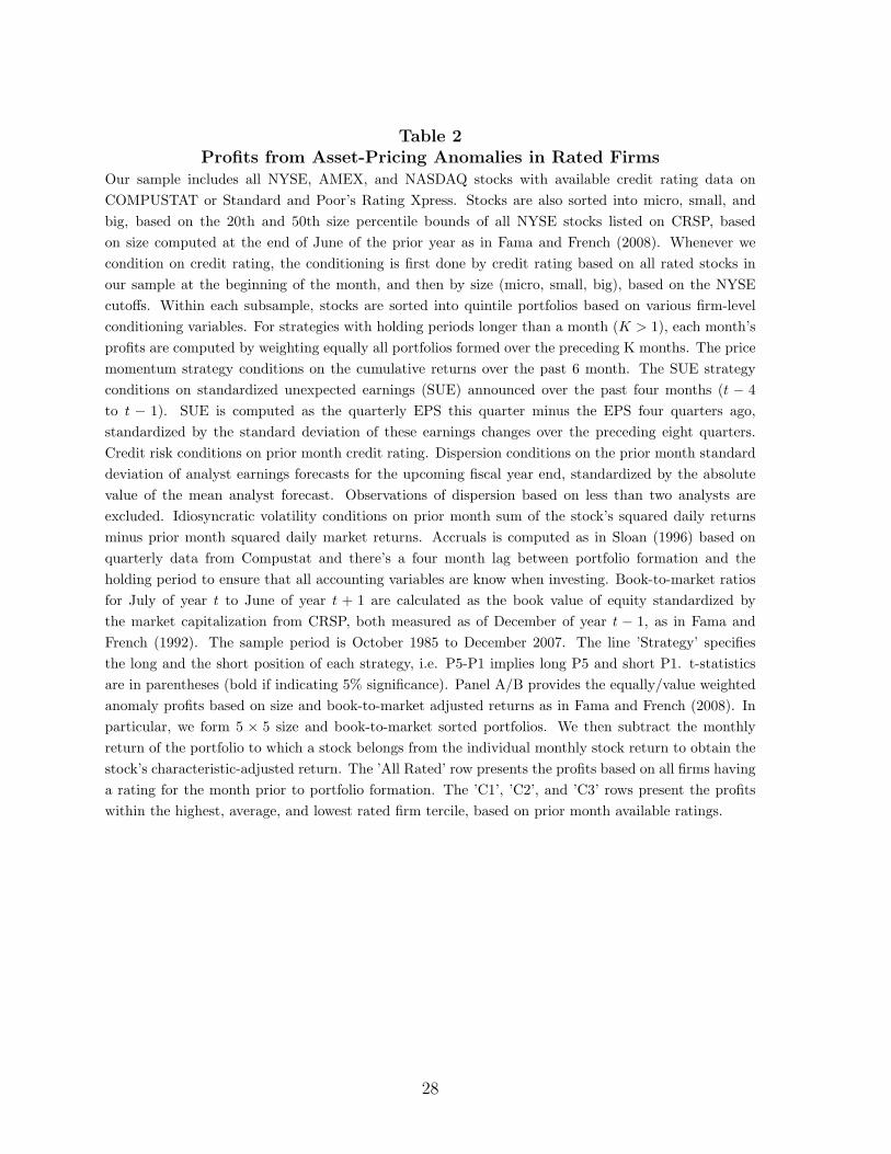
Table 2Profits from Asset-Pricing Anomalies in Rated Firms

Our sample includes all NYSE, AMEX, and NASDAQ stocks with available credit rating data onCOMPUSTAT or Standard and Poor’s Rating Xpress. Stocks are also sorted into micro, small, andbig, based on the 20th and 50th size percentile bounds of all NYSE stocks listed on CRSP, basedon size computed at the end of June of the prior year as in Fama and French (2008). Whenever wecondition on credit rating, the conditioning is first done by credit rating based on all rated stocks inour sample at the beginning of the month, and then by size (micro, small, big), based on the NYSEcutoffs. Within each subsample, stocks are sorted into quintile portfolios based on various firm-levelconditioning variables. For strategies with holding periods longer than a month (K > 1), each month’sprofits are computed by weighting equally all portfolios formed over the preceding K months. The pricemomentum strategy conditions on the cumulative returns over the past 6 month. The SUE strategyconditions on standardized unexpected earnings (SUE) announced over the past four months (t − 4to t − 1). SUE is computed as the quarterly EPS this quarter minus the EPS four quarters ago,standardized by the standard deviation of these earnings changes over the preceding eight quarters.Credit risk conditions on prior month credit rating. Dispersion conditions on the prior month standarddeviation of analyst earnings forecasts for the upcoming fiscal year end, standardized by the absolutevalue of the mean analyst forecast. Observations of dispersion based on less than two analysts areexcluded. Idiosyncratic volatility conditions on prior month sum of the stock’s squared daily returnsminus prior month squared daily market returns. Accruals is computed as in Sloan (1996) based onquarterly data from Compustat and there’s a four month lag between portfolio formation and theholding period to ensure that all accounting variables are know when investing. Book-to-market ratiosfor July of year t to June of year t + 1 are calculated as the book value of equity standardized bythe market capitalization from CRSP, both measured as of December of year t − 1, as in Fama andFrench (1992). The sample period is October 1985 to December 2007. The line ’Strategy’ specifiesthe long and the short position of each strategy, i.e. P5-P1 implies long P5 and short P1. t-statisticsare in parentheses (bold if indicating 5% significance). Panel A/B provides the equally/value weightedanomaly profits based on size and book-to-market adjusted returns as in Fama and French (2008). Inparticular, we form 5 × 5 size and book-to-market sorted portfolios. We then subtract the monthlyreturn of the portfolio to which a stock belongs from the individual monthly stock return to obtain thestock’s characteristic-adjusted return. The ’All Rated’ row presents the profits based on all firms havinga rating for the month prior to portfolio formation. The ’C1’, ’C2’, and ’C3’ rows present the profitswithin the highest, average, and lowest rated firm tercile, based on prior month available ratings.

28

Table 2 (continued)

Panel A: Equally Weighted Size and BM adjusted Returns

Anomaly Momentum SUE Credit Risk Dispersion Idio Vol Accruals BM

Strategy P5-P1 P5-P1 P1-P5 P1-P5 P1-P5 P1-P5 P5-P1

All Rated P1 -1.03 -0.49 0.03 0.09 -0.01 -0.18 -0.35P5 0.25 0.07 -0.87 -0.51 -1.08 -0.41 -0.16Strategy 1.28 0.57 0.91 0.60 1.06 0.23 0.19

(5.42) (4.48) (4.76) (3.14) (3.62) (3.22) (1.30)

Micro Rated P1 -1.62 -1.04 -0.21 -0.65 -0.07 -0.31 -0.72P5 0.53 0.22 -0.85 -0.91 -1.28 -0.60 -0.39Strategy 2.16 1.26 0.64 0.26 1.22 0.30 0.34

(8.86) (3.69) (1.96) (1.70) (3.64) (2.03) (0.64)

Small Rated P1 -1.14 -0.65 0.00 0.23 0.00 -0.25 -0.73P5 0.18 0.20 -0.88 -0.61 -1.02 -0.57 -0.12Strategy 1.33 0.85 0.88 0.84 1.02 0.32 0.60

(5.16) (4.49) (2.98) (3.66) (3.04) (2.78) (2.62)

Big Rated P1 -0.51 -0.23 0.05 0.09 -0.03 -0.05 -0.21P5 0.18 0.03 -0.60 -0.19 -0.78 -0.24 0.10Strategy 0.69 0.26 0.65 0.28 0.75 0.19 0.30

(2.44) (1.90) (1.89) (1.18) (2.01) (2.39) (1.78)

C1 All P1 0.02 -0.02 0.01 0.14 0.00 0.11 0.01P5 0.10 0.11 0.10 -0.01 -0.03 -0.04 -0.04Strategy 0.08 0.13 -0.09 0.15 0.03 0.15 -0.05

(0.47) (1.05) (-1.05) (0.96) (0.14) (2.71) (-0.29)

C1 Micro P1 -0.46 -0.35 -0.12 -1.03 0.60 0.27P5 0.13 0.61 -0.06 -0.13 -0.86 -0.34 -0.06Strategy 0.74 0.44 -0.07 -0.73 0.87 0.54

(1.74) (0.56) (-0.20) (-1.12) (1.76) (1.77)

C1 Small P1 -0.11 -0.35 -0.07 -0.01 0.03 -0.25 -0.72P5 -0.00 0.11 -0.06 -0.14 -0.40 -0.11 -0.00Strategy 0.11 0.43 -0.01 0.20 0.48 -0.15 0.89

(0.39) (1.18) (-0.03) (0.51) (1.71) (-0.91) (0.38)

C1 Big P1 0.06 0.02 0.02 0.17 -0.03 0.15 0.01P5 0.13 0.10 0.12 0.05 0.07 -0.01 -0.07Strategy 0.07 0.09 -0.10 0.12 -0.09 0.15 -0.08

(0.41) (0.68) (-1.02) (0.71) (-0.42) (2.53) (-0.46)

C2 All P1 -0.20 -0.21 0.00 0.08 -0.02 0.02 -0.05P5 0.21 0.05 0.01 0.03 -0.10 -0.24 0.02Strategy 0.41 0.26 -0.01 0.05 0.07 0.25 0.08

(2.22) (1.91) (-0.10) (0.30) (0.31) (3.05) (0.49)

C2 Micro P1 0.11 -0.57 0.03 -0.14 0.21 -0.07 3.32P5 -0.16 0.13 0.11 -0.16 -0.14 -0.26 -0.25Strategy -0.22 0.49 -0.19 -0.40 0.32 0.19 -4.08

(-0.55) (0.87) (-0.55) (-0.64) (0.74) (0.64) (-1.17)

C2 Small P1 -0.32 -0.24 -0.32 -0.00 -0.12 0.07 -0.45P5 0.20 0.18 -0.03 -0.12 -0.15 -0.26 -0.01Strategy 0.52 0.42 -0.30 0.12 0.03 0.33 0.44

(2.55) (2.18) (-1.79) (0.51) (0.12) (2.69) (0.98)

C2 Big P1 -0.22 -0.18 0.06 0.10 -0.01 -0.02 -0.05P5 0.26 0.02 0.01 0.08 -0.12 -0.26 0.10Strategy 0.47 0.20 0.05 0.02 0.12 0.24 0.15

(2.24) (1.35) (0.52) (0.10) (0.46) (2.34) (0.85)

C3 All P1 -2.10 -1.08 -0.12 -0.05 -0.10 -0.52 -0.89P5 0.43 0.12 -1.54 -0.80 -2.11 -0.79 -0.26Strategy 2.53 1.19 1.42 0.75 2.01 0.28 0.63

(7.45) (6.63) (6.59) (3.24) (6.24) (2.09) (2.33)

C3 Micro P1 -2.31 -1.35 -0.11 -0.58 0.05 -0.41 -0.72P5 0.74 0.08 -1.54 -1.25 -2.03 -0.77 -0.37Strategy 3.05 1.43 1.43 0.67 2.08 0.36 0.34

(9.34) (4.33) (4.55) (1.70) (6.06) (1.90) (0.69)

C3 Small P1 -2.02 -1.01 -0.09 0.19 -0.05 -0.50 -0.88P5 0.32 0.32 -1.49 -0.76 -2.18 -0.84 -0.19Strategy 2.35 1.33 1.40 0.95 2.13 0.35 0.69

(5.85) (5.41) (3.87) (3.13) (4.83) (1.95) (2.38)

C3 Big P1 -1.27 -0.75 -0.20 -0.29 -0.28 -0.50 -0.80P5 0.13 -0.08 -0.65 -0.43 -2.41 -0.98 0.50Strategy 1.40 0.66 0.45 0.14 2.13 0.48 1.29

(3.12) (2.18) (1.04) (0.43) (3.52) (1.64) (2.45)

29

Table 2 (continued)

Panel B: Value Weighted Size and BM adjusted Returns

Anomaly Momentum SUE Credit Risk Dispersion Idio Vol Accruals BM

Strategy P5-P1 P5-P1 P1-P5 P1-P5 P1-P5 P1-P5 P5-P1

All Rated P1 -0.44 -0.22 -0.04 -0.03 -0.11 -0.03 -0.16P5 0.12 -0.05 -0.91 -0.32 -0.55 -0.30 -0.05Strategy 0.56 0.17 0.86 0.29 0.43 0.27 0.11

(2.10) (0.95) (2.65) (1.06) (1.19) (2.41) (0.59)

Micro Rated P1 -1.60 -1.06 -0.28 -0.79 -0.07 -0.37 -0.62P5 0.35 0.05 -0.98 -1.03 -1.42 -0.57 -0.27Strategy 1.95 1.11 0.70 0.21 1.36 0.19 0.37

(7.56) (3.35) (1.92) (0.52) (3.84) (1.33) (0.64)

Small Rated P1 -1.21 -0.67 0.02 0.22 -0.00 -0.20 -0.69P5 0.21 0.12 -0.98 -0.64 -1.10 -0.58 -0.13Strategy 1.42 0.79 1.00 0.87 1.10 0.38 0.56

(5.18) (3.99) (3.16) (3.66) (3.07) (3.13) (2.37)

Big Rated P1 -0.35 -0.20 -0.04 -0.04 -0.12 -0.02 -0.15P5 0.11 -0.05 -0.59 -0.26 -0.41 -0.27 -0.05Strategy 0.46 0.14 0.55 0.22 0.29 0.26 0.10

(1.68) (0.78) (1.43) (0.79) (0.76) (2.26) (0.55)

C1 All P1 -0.06 -0.10 -0.04 0.13 -0.06 0.06 -0.08P5 0.03 0.04 -0.05 -0.04 -0.14 -0.16 -0.10Strategy 0.09 0.14 0.01 0.17 0.08 0.22 -0.02

(0.43) (0.73) (0.08) (0.67) (0.31) (2.01) (-0.13)

C1 Micro P1 -0.50 -0.45 0.00 -1.06 0.57 0.27P5 -0.06 0.55 -0.30 0.07 -1.00 -0.37 0.04Strategy 0.57 0.62 0.30 -0.81 1.01 0.54

(1.37) (0.77) (0.73) (-1.09) (1.91) (1.88)

C1 Small P1 -0.03 -0.33 -0.02 -0.04 0.03 -0.23 -0.72P5 0.01 0.11 -0.04 -0.21 -0.27 -0.11 0.03Strategy 0.04 0.41 0.02 0.24 0.36 -0.11 1.22

(0.15) (1.12) (0.11) (0.59) (1.22) (-0.71) (0.54)

C1 Big P1 -0.07 -0.09 -0.04 0.13 -0.06 0.06 -0.08P5 0.03 0.04 -0.06 -0.04 -0.14 -0.15 -0.11Strategy 0.10 0.13 0.01 0.17 0.08 0.22 -0.03

(0.44) (0.71) (0.08) (0.65) (0.29) (2.00) (-0.15)

C2 All P1 -0.40 -0.40 -0.03 0.07 0.02 -0.10 -0.17P5 0.34 -0.20 -0.11 -0.21 -0.30 -0.45 -0.06Strategy 0.74 0.20 0.08 0.27 0.32 0.35 0.10

(2.82) (0.93) (0.63) (0.96) (0.97) (2.77) (0.44)

C2 Micro P1 -0.06 -0.64 -0.03 -0.16 0.04 -0.24 3.51P5 -0.22 0.14 -0.24 -0.60 -0.33 -0.30 -0.38Strategy -0.10 0.55 0.07 0.11 0.34 0.06 -4.33

(-0.23) (0.94) (0.21) (0.16) (0.75) (0.20) (-1.25)

C2 Small P1 -0.33 -0.26 -0.29 0.07 -0.10 0.11 -0.51P5 0.20 0.17 -0.07 -0.12 -0.25 -0.23 -0.02Strategy 0.53 0.43 -0.22 0.19 0.14 0.33 0.49

(2.50) (2.08) (-1.32) (0.76) (0.54) (2.40) (1.06)

C2 Big P1 -0.40 -0.40 -0.03 0.07 0.03 -0.12 -0.16P5 0.35 -0.21 -0.10 -0.21 -0.29 -0.46 -0.06Strategy 0.75 0.20 0.08 0.27 0.33 0.35 0.10

(2.79) (0.89) (0.56) (0.93) (0.97) (2.63) (0.43)

C3 All P1 -1.58 -0.95 -0.32 -0.26 -0.23 -0.81 -0.81P5 0.21 -0.10 -1.39 -0.61 -2.10 -0.96 0.23Strategy 1.79 0.85 1.07 0.35 1.87 0.15 1.04

(4.28) (3.05) (3.08) (1.18) (4.04) (0.69) (2.47)

C3 Micro P1 -2.31 -1.38 -0.12 -0.66 0.01 -0.49 -0.93P5 0.49 -0.13 -1.65 -1.25 -2.41 -0.72 -0.18Strategy 2.80 1.25 1.53 0.59 2.41 0.24 0.75

(7.96) (3.79) (4.42) (1.37) (6.41) (1.30) (1.36)

C3 Small P1 -2.20 -1.03 -0.09 0.18 -0.10 -0.47 -0.80P5 0.35 0.21 -1.62 -0.81 -2.27 -0.93 -0.19Strategy 2.55 1.24 1.53 0.99 2.17 0.46 0.61

(5.98) (4.57) (3.90) (3.07) (4.54) (2.35) (2.03)

C3 Big P1 -1.10 -0.78 -0.32 -0.44 -0.28 -0.74 -0.77P5 0.13 -0.16 -0.63 -0.50 -2.25 -0.97 0.29Strategy 1.23 0.62 0.30 0.06 1.97 0.23 1.06

(2.65) (1.79) (0.65) (0.17) (3.09) (0.77) (1.66)

30

Table 3Profits from Asset-Pricing Anomalies

in Decreasing Subsamples of Rated FirmsWe repeat the analysis in Table 2 sequentially eliminating the worst rated stocks. The results presentedhere are based on equally weighted size and BM adjusted returns.

Anomaly Momentum SUE Credit Risk Dispersion Idio Vol Accruals BM % of Firms % of MV

All (AAA-D) 1.28 0.57 0.91 0.60 1.06 0.23 0.19 100.00 100.00(5.42) (4.48) (4.76) (3.14) (3.62) (3.22) (1.30)

Micro (AAA-D) 2.16 1.26 0.64 0.26 1.22 0.30 0.34 17.81 0.43(8.86) (3.69) (1.96) (1.70) (3.64) (2.03) (0.64)

Small (AAA-D) 1.33 0.85 0.88 0.84 1.02 0.32 0.60 27.07 2.97(5.16) (4.49) (2.98) (3.66) (3.04) (2.78) (2.62)

Big (AAA-D) 0.69 0.26 0.65 0.28 0.75 0.19 0.30 55.12 96.59(2.44) (1.90) (1.89) (1.18) (2.01) (2.39) (1.78)

All (AAA-C) 1.20 0.55 0.75 0.54 0.91 0.25 0.23 99.10 99.93(5.14) (4.37) (4.02) (2.84) (3.07) (3.54) (1.57)

Micro (AAA-C) 2.01 1.21 0.44 0.20 0.96 0.37 0.45 17.06 0.42(8.34) (3.64) (1.26) (0.54) (2.84) (2.59) (0.85)

Small (AAA-C) 1.28 0.84 0.76 0.79 0.91 0.33 0.60 26.97 2.96(5.06) (4.47) (2.70) (3.46) (2.76) (2.92) (2.63)

Big (AAA-C) 0.67 0.26 0.56 0.25 0.68 0.18 0.31 55.07 96.54(2.41) (1.88) (1.67) (1.07) (1.84) (2.24) (1.84)

All (AAA-CC) 1.20 0.55 0.75 0.54 0.90 0.25 0.23 99.09 99.93(5.14) (4.37) (4.01) (2.84) (3.06) (3.54) (1.59)

Micro (AAA-CC) 2.01 1.21 0.43 0.20 0.95 0.37 0.45 17.06 0.42(8.34) (3.64) (1.25) (0.54) (2.82) (2.60) (0.87)

Small (AAA-CC) 1.27 0.84 0.76 0.79 0.91 0.33 0.60 26.97 2.96(5.06) (4.47) (2.70) (3.46) (2.75) (2.91) (2.63)

Big (AAA-CC) 0.67 0.26 0.56 0.25 0.68 0.18 0.31 55.07 96.54(2.41) (1.88) (1.67) (1.07) (1.85) (2.24) (1.85)

All (AAA-CCC-) 1.18 0.54 0.71 0.54 0.87 0.26 0.23 98.87 99.91(5.05) (4.26) (3.83) (2.83) (2.94) (3.69) (1.62)

Micro (AAA-CCC-) 1.95 1.20 0.39 0.21 0.89 0.42 0.33 16.89 0.42(8.14) (3.51) (1.11) (0.57) (2.64) (2.97) (0.61)

Small (AAA-CCC-) 1.26 0.83 0.73 0.79 0.91 0.33 0.59 26.93 2.96(5.04) (4.41) (2.60) (3.45) (2.74) (2.92) (2.58)

Big (AAA-CCC-) 0.66 0.25 0.56 0.26 0.66 0.18 0.31 55.05 96.53(2.40) (1.81) (1.69) (1.10) (1.80) (2.25) (1.86)

All (AAA-CCC) 1.16 0.54 0.67 0.53 0.84 0.26 0.25 98.62 99.90(4.99) (4.28) (3.63) (2.80) (2.84) (3.75) (1.76)

Micro (AAA-CCC) 1.89 1.24 0.35 0.20 0.84 0.43 0.39 16.70 0.42(7.91) (3.57) (1.03) (0.54) (2.50) (3.03) (0.71)

Small (AAA-CCC) 1.26 0.82 0.67 0.79 0.89 0.32 0.59 26.88 2.96(5.06) (4.41) (2.41) (3.44) (2.69) (2.89) (2.59)

Big (AAA-CCC) 0.66 0.25 0.52 0.26 0.65 0.18 0.32 55.04 96.52(2.39) (1.83) (1.57) (1.09) (1.79) (2.24) (1.91)

All (AAA-CCC+) 1.11 0.51 0.60 0.50 0.75 0.27 0.29 98.03 99.86(4.78) (4.05) (3.45) (2.65) (2.58) (3.84) (2.03)

Micro (AAA-CCC+) 1.76 1.12 0.27 0.22 0.69 0.45 0.37 16.30 0.41(7.38) (3.22) (0.81) (0.60) (2.09) (3.25) (0.69)

Small (AAA-CCC+) 1.24 0.81 0.63 0.74 0.84 0.32 0.60 26.75 2.95(5.03) (4.33) (2.36) (3.22) (2.58) (2.89) (2.59)

Big (AAA-CCC+) 0.64 0.24 0.47 0.26 0.63 0.18 0.31 54.98 96.49(2.36) (1.73) (1.46) (1.10) (1.74) (2.25) (1.85)

All (AAA-B-) 1.03 0.48 0.52 0.45 0.65 0.27 0.26 97.07 99.78(4.52) (3.79) (3.07) (2.39) (2.29) (3.96) (1.86)

Micro (AAA-B-) 1.61 1.03 0.21 0.10 0.61 0.47 0.08 15.67 0.40(6.84) (2.99) (0.62) (0.28) (1.92) (3.49) (0.14)

Small (AAA-B-) 1.16 0.78 0.54 0.67 0.70 0.32 0.59 26.52 2.93(4.79) (4.15) (2.07) (3.00) (2.23) (2.90) (2.52)

Big (AAA-B-) 0.62 0.23 0.47 0.24 0.57 0.18 0.29 54.88 96.45(2.32) (1.67) (1.52) (1.05) (1.61) (2.30) (1.76)

31

Table 3 (continued)

Anomaly Momentum SUE Credit Risk Dispersion Idio Vol Accruals BM % of Firms % of MV

All (AAA-B) 0.90 0.43 0.45 0.41 0.53 0.29 0.21 94.74 99.44(4.17) (3.50) (2.85) (2.27) (1.94) (4.33) (1.55)

Micro (AAA-B) 1.40 1.09 0.11 0.16 0.52 0.46 0.15 14.41 0.37(6.38) (3.36) (0.35) (0.45) (1.68) (3.47) (0.24)

Small (AAA-B) 1.03 0.75 0.49 0.62 0.58 0.34 0.49 25.79 2.85(4.51) (3.96) (1.91) (2.84) (1.93) (3.09) (2.10)

Big (AAA-B) 0.54 0.17 0.39 0.22 0.46 0.22 0.24 54.54 96.21(2.11) (1.30) (1.35) (0.95) (1.37) (3.01) (1.56)

All (AAA-B+) 0.73 0.38 0.35 0.33 0.37 0.32 0.16 90.34 98.72(3.65) (3.19) (2.42) (1.86) (1.47) (4.74) (1.21)

Micro (AAA-B+) 1.18 1.36 0.05 -0.02 0.39 0.55 0.54 12.04 0.32(5.60) (3.81) (0.16) (-0.05) (1.32) (3.98) (0.91)

Small (AAA-B+) 0.84 0.64 0.40 0.50 0.39 0.38 0.39 24.43 2.72(3.98) (3.48) (1.63) (2.31) (1.43) (3.53) (1.67)

Big (AAA-B+) 0.47 0.16 0.29 0.20 0.29 0.24 0.17 53.87 95.69(1.97) (1.23) (1.13) (0.88) (0.93) (3.27) (1.15)

All (AAA-BB-) 0.52 0.27 0.16 0.22 0.19 0.27 0.12 80.93 97.42(2.77) (2.45) (1.21) (1.29) (0.79) (4.48) (0.96)

Micro (AAA-BB-) 0.84 0.96 -0.10 -0.23 0.32 0.34 -0.93 8.00 0.21(3.17) (2.26) (-0.29) (-0.54) (0.98) (1.84) (-1.09)

Small (AAA-BB-) 0.66 0.49 0.14 0.25 0.26 0.34 0.35 20.55 2.35(3.41) (2.70) (0.59) (1.28) (1.00) (3.32) (1.34)

Big (AAA-BB-) 0.37 0.14 0.26 0.18 0.13 0.23 0.07 52.38 94.86(1.73) (1.16) (1.36) (0.87) (0.49) (3.47) (0.51)

All (AAA-BB) 0.40 0.26 0.05 0.19 0.10 0.24 0.10 72.16 95.68(2.22) (2.26) (0.40) (1.14) (0.42) (3.96) (0.78)

Micro (AAA-BB) 0.54 0.84 -0.18 -0.02 0.37 0.27 -1.74 5.57 0.14(1.83) (1.85) (-0.53) (-0.04) (1.06) (1.12) (-0.87)

Small (AAA-BB) 0.53 0.54 0.06 0.17 0.13 0.29 0.11 16.30 1.87(2.82) (2.85) (0.27) (0.89) (0.54) (2.97) (0.23)

Big (AAA-BB) 0.33 0.16 0.09 0.18 0.07 0.22 0.05 50.29 93.67(1.67) (1.30) (0.60) (0.90) (0.27) (3.27) (0.38)

All (AAA-BB+) 0.30 0.21 0.05 0.19 0.06 0.19 -0.03 65.24 93.69(1.75) (1.94) (0.50) (1.18) (0.29) (3.58) (-0.20)

Micro (AAA-BB+) 0.25 1.35 -0.06 -0.47 0.26 0.09 7.04 4.63 0.11(0.82) (2.23) (-0.17) (-1.00) (0.70) (0.34) (2.63)

Small (AAA-BB+) 0.40 0.47 0.10 0.13 0.13 0.16 0.10 12.93 1.47(2.21) (2.51) (0.51) (0.66) (0.58) (1.65) (0.17)

Big (AAA-BB+) 0.29 0.15 0.08 0.20 0.02 0.21 -0.03 47.68 92.11(1.57) (1.28) (0.67) (1.07) (0.08) (3.36) (-0.21)

All (AAA-BBB-) 0.23 0.14 0.05 0.14 0.07 0.19 -0.02 59.79 91.20(1.36) (1.30) (0.56) (0.91) (0.33) (3.57) (-0.16)

Micro (AAA-BBB-) 0.16 0.69 0.19 -0.15 0.87 -0.09 4.03 0.09(0.53) (1.26) (0.57) (-0.29) (1.39) (-0.31)

Small (AAA-BBB-) 0.29 0.39 0.10 0.08 0.15 0.19 0.14 10.97 1.25(1.59) (2.11) (0.55) (0.38) (0.67) (1.70) (0.22)

Big (AAA-BBB-) 0.23 0.09 0.04 0.13 -0.01 0.19 -0.06 44.79 89.86(1.30) (0.78) (0.39) (0.72) (-0.03) (3.07) (-0.42)

All (AAA-BBB) 0.19 0.15 0.06 0.15 -0.00 0.19 0.01 51.51 86.70(1.12) (1.35) (0.64) (0.97) (-0.01) (3.25) (0.06)

Micro (AAA-BBB) 0.16 0.44 -0.06 -0.12 0.50 0.07 3.54 0.08(0.50) (0.83) (-0.15) (-0.23) (1.28) (0.25)

Small (AAA-BBB) 0.17 0.28 0.05 -0.21 0.13 0.15 0.13 8.28 0.90(0.87) (1.39) (0.28) (-0.91) (0.56) (1.18) (0.14)

Big (AAA-BBB) 0.20 0.12 0.07 0.17 -0.06 0.18 -0.01 39.70 85.72(1.12) (1.03) (0.73) (0.97) (-0.29) (2.84) (-0.08)

32

Table 4Downgrade Characteristics, Delistings, and Returns by Credit Rating GroupsThe table focuses on stocks with at least one downgrade. Panel A analyzes downgrades by credit ratingtercile, sorted on firm rating at the end of month t−1. We also report statistics for up/down markets (whenthe excess value-weighted market return is positive/negative), as well as for expansions and recessions asdefined by NBER. The downgrade correlation is the average pairwise time-series correlation between anytwo stocks in a given rating tercile. This correlation is computed based on an index for each stock whichtakes the value of 0/1 during months with no/one downgrade. Also reported are downgrade correlationscomputed based on dummies taking the value of 1 three (six) months before and after downgrades. PanelB divides firms by number of downgrades and for each downgrade frequency, analyzes investment-grade(IG) and non-investment grade (NIG) firms. The sample period is October 1985 to December 2007.

PANEL A: By Credit Rating PortfolioRating Group (C1=Lowest , C3=Highest Risk)

C1 C2 C3Number of Downgrades 2,276 2,363 3,286Downgrades/month 8.56 8.88 12.35Size of Downgrades 1.77 1.77 2.24

rt−1 0.75 -3.09 -12.04rt -0.34 -2.23 -15.21rt+1 0.76 0.42 -3.52rt−6:t−1 3.64 -6.37 -29.38rt+1:t+6 7.55 0.47 -16.73rt−12:t−1 7.59 -3.92 -31.95rt+1:t+12 13.15 4.41 -11.72rt−24:t−1 21.04 0.27 -28.92rt+1:t+24 28.95 19.52 9.49Delisted over (t + 1 : t + 6) 53 105 379Delisted over (t + 1 : t + 12) 85 165 601Delisted over (t + 1 : t + 24) 138 298 847

Downgrades/month (rmt > 0) 7.64 7.90 10.61Size of Downgrades 1.71 1.83 2.27

rt−1 1.35 -3.56 -12.22rt 1.83 1.71 -10.80rt+1 1.69 0.91 0.32

Downgrades/month (rmt < 0) 10.16 10.31 15.30Size of Downgrades 1.85 1.66 2.18

rt−1 -0.16 -2.42 -11.77rt -3.61 -7.84 -22.24rt+1 -0.67 -0.29 -9.77

Downgrades/month (Expansions) 8.19 8.61 11.59Size of Downgrades 1.72 1.76 2.20

rt−1 0.84 -1.96 -11.51rt 0.16 -2.01 -15.59rt+1 0.18 0.64 -3.29

Downgrades/month (Recessions) 13.00 13.93 25.87Size of Downgrades 1.90 1.68 2.97

rt−1 -0.55 -16.25 -19.13rt -7.45 -4.80 -10.30rt+1 8.93 -2.10 -6.38

Downgrade Correlation (%) 2.31 4.23 7.48Downgrade Correlation (±3 months) (%) 1.59 1.87 3.96Downgrade Correlation (±6 months) (%) 1.87 2.21 4.68

33

Table 4 (continued)

PANEL B: By Frequency of Downgrades

# of Firms Size Months Returns Around Each DowngradeDowngr. with N of Each Betweenper Firm Downgr. Downgr. Downgr. rt−3:t−1 rt:t+3 rt−6:t−1 rt:t+6

IG NIG IG NIG IG NIG IG NIG IG NIG IG NIG IG NIG

N=1 577 583 1.99 2.35 -0.04 -14.58 -0.25 -13.59 1.95 -21.96 3.07 -12.34N=2 318 357 1.72 2.22 45.71 18.48 -0.75 -14.87 0.93 -18.77 -1.42 -24.61 5.70 -20.09N=3 204 191 1.51 1.91 38.19 18.05 -0.72 -16.41 -0.83 -20.17 -1.02 -26.35 2.59 -22.88N=4 118 99 1.39 1.70 34.33 18.79 -2.53 -14.58 0.76 -14.21 -2.32 -17.19 5.84 -22.50N=5 47 30 1.36 1.69 33.84 15.57 -3.56 -17.80 0.19 -10.75 -5.82 -25.75 2.78 -9.90N=6 17 8 1.37 1.42 30.24 13.20 -2.56 -16.64 -0.24 -20.78 0.03 -29.76 2.72 -21.69N=7 7 2 1.22 1.79 26.00 22.00 -1.33 -4.11 -0.89 -10.03 -2.67 -14.66 4.26 2.86N=8 1 1 1.25 1.00 27.86 34.29 4.10 -1.36 20.03 20.74 3.20 -6.95 33.51 27.05N=9 1 1.33 27.75 -13.98 11.30 -19.36 17.39N=10 1 2.20 13.89 1.03 7.15 -0.86 14.40

Obs. 8,112 7,432 10,605 9,491 16,196 14,824 18,105 15,665

34

Table 5Impact of Downgrades on Profits from Asset-Pricing Anomalies

We repeat the analysis described in Table 2 after removing 6-months of returns before and after rating downgrades.

Panel A: Equally Weighted Size and BM adjusted Returns

Anomaly Momentum SUE Credit Risk Dispersion Idio Vol Accruals BM

Strategy P5-P1 P5-P1 P1-P5 P1-P5 P1-P5 P1-P5 P5-P1

All Rated P1 0.09 0.16 0.11 0.16 0.07 0.38 -0.07P5 0.37 0.22 0.05 0.28 0.05 0.02 0.36Strategy 0.28 0.05 0.06 -0.12 0.02 0.36 0.43

(1.22) (0.43) (0.34) (-0.64) (0.07) (4.99) (2.79)

Micro Rated P1 0.25 0.24 -0.30 -0.40 -0.04 0.92 0.12P5 0.69 0.69 0.35 0.37 0.43 0.16 0.48Strategy 0.44 0.45 -0.64 -0.77 -0.46 0.76 0.40

(1.77) (1.18) (-1.65) (-1.57) (-1.32) (4.18) (0.73)

Small Rated P1 -0.02 0.11 0.04 0.31 0.10 0.28 -0.25P5 0.36 0.42 -0.05 0.35 0.00 -0.05 0.34Strategy 0.38 0.31 0.08 -0.04 0.10 0.33 0.59

(1.61) (1.69) (0.31) (-0.18) (0.30) (2.75) (2.48)

Big Rated P1 0.17 0.17 0.14 0.15 0.06 0.22 -0.01P5 0.25 0.13 -0.11 0.21 -0.16 0.00 0.27Strategy 0.08 -0.04 0.24 -0.06 0.22 0.22 0.28

(0.29) (-0.28) (0.76) (-0.27) (0.60) (3.03) (1.67)

C1 All P1 0.18 0.10 0.07 0.17 0.06 0.19 0.07P5 0.13 0.15 0.18 0.12 0.14 0.04 0.06Strategy -0.05 0.05 -0.11 0.05 -0.07 0.15 -0.01

(-0.30) (0.38) (-1.27) (0.28) (-0.35) (2.74) (-0.03)

C1 Micro P1 -0.71 -0.40 -0.28 -1.04 0.47 0.19P5 0.04 0.36 -0.13 -0.45 -0.83 -0.42 0.16Strategy 0.91 0.46 -0.17 -0.35 0.69 0.59

(1.87) (0.56) (-0.41) (-0.56) (1.26) (1.89)

C1 Small P1 0.02 -0.20 0.00 -0.02 0.09 -0.21 -0.72P5 -0.05 0.23 0.01 -0.03 -0.44 -0.20 0.00Strategy -0.07 0.43 -0.01 0.09 0.53 -0.02 0.69

(-0.26) (1.06) (-0.04) (0.22) (1.85) (-0.12) (0.29)

C1 Big P1 0.24 0.15 0.09 0.20 0.04 0.24 0.07P5 0.16 0.15 0.22 0.19 0.24 0.09 0.05Strategy -0.07 -0.01 -0.13 0.01 -0.20 0.15 -0.02

(-0.41) (-0.04) (-1.25) (0.05) (-0.89) (2.43) (-0.10)

C2 All P1 0.31 0.13 0.12 0.16 0.07 0.24 0.12P5 0.26 0.17 0.25 0.30 0.26 0.01 0.24Strategy -0.04 0.04 -0.12 -0.14 -0.19 0.23 0.12

(-0.25) (0.29) (-1.54) (-0.82) (-0.81) (2.72) (0.70)

C2 Micro P1 0.21 -0.61 -0.25 -0.12 0.18 0.19 3.89P5 -0.04 -0.12 0.16 0.18 0.01 -0.22 -0.38Strategy -0.21 0.12 -0.45 -0.49 0.10 0.43 -4.71

(-0.54) (0.19) (-1.19) (-0.67) (0.20) (1.47) (-1.26)

C2 Small P1 0.29 0.06 -0.17 0.14 -0.03 0.26 -0.23P5 0.31 0.30 0.33 0.31 0.30 0.07 0.29Strategy 0.02 0.24 -0.50 -0.17 -0.34 0.19 0.52

(0.10) (1.31) (-1.06) (-0.68) (-1.31) (1.45) (1.15)

C2 Big P1 0.28 0.21 0.20 0.16 0.11 0.20 0.10P5 0.30 0.15 0.21 0.32 0.24 -0.02 0.28Strategy 0.02 -0.06 -0.00 -0.16 -0.13 0.23 0.18

(0.09) (-0.40) (-0.05) (-0.78) (-0.51) (2.18) (0.94)

C3 All P1 -0.02 0.13 0.22 0.09 0.13 0.56 -0.32P5 0.62 0.44 0.08 0.48 -0.04 0.02 0.70Strategy 0.64 0.30 0.14 -0.39 0.17 0.54 1.03

(1.81) (1.60) (0.67) (-1.57) (0.48) (3.88) (3.70)

C3 Micro P1 0.55 0.17 0.30 -0.44 0.27 0.94 -0.01P5 0.93 0.60 0.45 0.62 0.62 0.15 0.75Strategy 0.38 0.43 -0.15 -1.07 -0.35 0.80 0.76

(1.06) (1.17) (-0.45) (-1.15) (-0.88) (3.45) (1.42)

C3 Small P1 -0.42 0.12 0.28 0.31 0.21 0.39 -0.37P5 0.51 0.61 0.08 0.53 -0.49 -0.11 0.60Strategy 0.93 0.49 0.20 -0.22 0.70 0.50 0.97

(2.37) (1.99) (0.61) (-0.73) (1.55) (2.50) (3.16)

C3 Big P1 0.05 0.18 0.10 -0.20 -0.10 0.23 -0.38P5 0.29 0.14 -0.34 0.45 -1.03 -0.17 0.91Strategy 0.23 -0.03 0.44 -0.66 0.96 0.40 1.27

(0.52) (-0.11) (1.08) (-1.86) (1.49) (1.45) (2.19)

35

Table 5 (continued)

Panel B: Value Weighted Size and BM adjusted Returns

Anomaly Momentum SUE Credit Risk Dispersion Idio Vol Accruals BM

Strategy P5-P1 P5-P1 P1-P5 P1-P5 P1-P5 P1-P5 P5-P1

All Rated P1 0.08 0.14 0.06 0.03 -0.03 0.19 -0.05P5 0.16 0.02 -0.16 0.12 -0.01 -0.10 0.14Strategy 0.08 -0.13 0.22 -0.08 -0.02 0.28 0.18

(0.31) (-0.77) (0.69) (-0.32) (-0.06) (2.54) (1.06)

Micro Rated P1 0.19 0.18 -0.19 -0.38 -0.06 0.73 0.04P5 0.53 0.39 0.18 0.09 0.28 0.13 0.52Strategy 0.34 0.21 -0.37 -0.48 -0.33 0.60 0.52

(1.28) (0.59) (-1.06) (-1.17) (-0.89) (3.35) (0.92)

Small Rated P1 -0.03 0.12 0.06 0.31 0.09 0.32 -0.17P5 0.37 0.35 -0.04 0.37 0.01 -0.07 0.30Strategy 0.40 0.23 0.10 -0.06 0.08 0.39 0.47

(1.62) (1.23) (0.36) (-0.24) (0.24) (3.28) (1.90)

Big Rated P1 0.10 0.14 0.06 0.03 -0.04 0.19 -0.04P5 0.15 0.01 -0.03 0.09 0.01 -0.09 0.10Strategy 0.05 -0.13 0.09 -0.06 -0.04 0.28 0.14

(0.18) (-0.78) (0.23) (-0.23) (-0.11) (2.41) (0.77)

C1 All P1 0.19 0.12 0.03 0.15 0.02 0.20 -0.02P5 0.07 0.09 0.08 0.13 0.09 -0.05 0.06Strategy -0.11 -0.03 -0.04 0.02 -0.07 0.25 0.08

(-0.51) (-0.14) (-0.25) (0.09) (-0.24) (2.20) (0.41)

C1 Micro P1 -0.73 -0.51 -0.08 -1.07 0.44 0.20P5 -0.08 0.33 -0.24 -0.25 -0.91 -0.44 0.28Strategy 0.79 0.73 0.15 -0.56 0.84 0.62

(1.85) (0.87) (0.33) (-0.79) (1.45) (2.05)

C1 Small P1 0.11 -0.21 0.06 -0.06 0.10 -0.20 -0.72P5 -0.03 0.22 0.02 -0.07 -0.29 -0.18 0.02Strategy -0.14 0.43 0.04 0.09 0.39 -0.02 1.01

(-0.50) (1.08) (0.20) (0.21) (1.30) (-0.11) (0.45)

C1 Big P1 0.18 0.12 0.03 0.15 0.02 0.21 -0.02P5 0.08 0.09 0.08 0.13 0.09 -0.04 0.06Strategy -0.11 -0.03 -0.04 0.02 -0.07 0.25 0.08

(-0.49) (-0.16) (-0.25) (0.09) (-0.25) (2.20) (0.39)

C2 All P1 0.02 0.03 0.10 0.19 0.14 0.06 0.04P5 0.37 -0.04 0.16 0.13 0.03 -0.22 0.08Strategy 0.35 -0.06 -0.05 0.07 0.11 0.28 0.04

(1.35) (-0.33) (-0.43) (0.24) (0.34) (2.12) (0.17)

C2 Micro P1 0.14 -0.74 -0.33 -0.13 0.02 -0.00 3.89P5 -0.12 -0.10 -0.15 -0.11 0.06 -0.23 -0.50Strategy -0.22 0.27 -0.22 -0.38 -0.13 0.25 -4.70

(-0.52) (0.43) (-0.59) (-0.46) (-0.23) (0.92) (-1.25)

C2 Small P1 0.24 0.04 -0.12 0.24 -0.03 0.27 -0.20P5 0.29 0.29 0.27 0.31 0.22 0.13 0.25Strategy 0.04 0.25 -0.39 -0.07 -0.25 0.15 0.45

(0.21) (1.27) (-1.30) (-0.26) (-0.94) (1.01) (0.95)

C2 Big P1 0.01 0.03 0.11 0.19 0.16 0.04 0.04P5 0.38 -0.05 0.16 0.12 0.02 -0.24 0.07Strategy 0.37 -0.07 -0.05 0.07 0.13 0.28 0.03

(1.40) (-0.36) (-0.37) (0.24) (0.39) (2.01) (0.14)

C3 All P1 -0.15 0.01 -0.07 -0.06 0.00 0.14 -0.33P5 0.35 0.12 -0.32 0.36 -0.67 -0.12 0.88Strategy 0.50 0.11 0.25 -0.42 0.67 0.26 1.21

(1.19) (0.40) (0.83) (-1.35) (1.41) (1.29) (2.77)

C3 Micro P1 0.38 0.10 0.32 -0.40 0.20 0.76 -0.06P5 0.71 0.25 0.50 0.25 0.59 0.13 0.93Strategy 0.33 0.15 -0.17 -0.65 -0.39 0.63 1.00

(0.88) (0.42) (-0.49) (-1.31) (-0.83) (2.88) (1.70)

C3 Small P1 -0.45 0.20 0.28 0.31 0.14 0.43 -0.26P5 0.54 0.53 0.07 0.55 -0.51 -0.15 0.61Strategy 0.99 0.33 0.22 -0.24 0.65 0.58 0.86

(2.36) (1.29) (0.63) (-0.76) (1.34) (2.96) (2.71)

C3 Big P1 0.03 0.01 -0.13 -0.28 -0.04 0.09 -0.34P5 0.25 0.04 -0.35 0.34 -1.11 -0.15 0.74Strategy 0.22 0.03 0.22 -0.62 1.09 0.24 1.04

(0.47) (0.08) (0.52) (-1.62) (1.60) (0.82) (1.50)

36

Table 6Cross-Sectional Regressions

Each month t, we run univariate cross-sectional regressions of monthly risk-adjusted stock returns on alagged firm characteristic based on each of the anomalies studied using all NYSE, AMEX, and NASDAQstocks with available credit rating data on COMPUSTAT or Standard and Poor’s Rating Xpress:

r∗it = at + btCit−1 + eit.

Each firm characteristic, Cit−1, is a conditioning variable described in Table 2. Each column reports theresults from a separate univariate regression and shows the time-series average of these cross-sectionalregression coefficients, bt, with their associated sample t-statistics in parentheses (bold if significant atthe 95% confidence level). We use risk-adjusted returns as dependent variable, i.e. the constant anderror term obtained from time-series regressions of raw excess returns on the Fama and French (1993)factors: r∗it = Rit − Rft −

∑Kk=1 β̂ikFkt. Each panel also provides results where in the regression for

each anomaly we include dummies indicating rating downgrades:

r∗it = at + btCit−1 + dt,IGDIG + dt,NIGDNIG + eit,

where DIG (DNIG) is a dummy variable which takes the value of 1 from 6 months before to 6 monthsafter rating downgrades from an investment-grade (non-investment-grade) rating. Panel A presentsresults for all stocks, while Panel B/C/D show results for Micro/Small/Big stocks, respectively.

Panel A: Risk-Adjusted Returns: All Stocks

Momentum SUE Credit Risk Dispersion Idio Vol Accruals Size BM

b 0.90 0.14 -0.09 -0.23 -6.03 -2.42 -0.05 0.02(3.30) (5.04) (-5.17) (-3.77) (-2.86) (-2.41) (-1.54) (0.20)

b 0.19 0.05 -0.01 -0.02 -4.87 -3.67 -0.04 0.28(0.63) (2.12) (-0.71) (-0.31) (-1.70) (-3.27) (-1.60) (2.69)

dNIG -4.07 -3.70 -3.93 -4.29 -3.92 -3.65 -4.04 -3.35(-16.57) (-11.52) (-15.69) (-13.44) (-16.65) (-12.26) (-14.65) (-10.00)

b 0.09 0.04 -0.02 -0.01 -5.16 -3.69 -0.02 0.32(0.31) (1.53) (-1.49) (-0.13) (-1.81) (-3.30) (-1.01) (3.00)

dIG -0.83 -0.87 -0.87 -0.81 -0.86 -0.79 -0.82 -0.82(-9.35) (-9.00) (-8.64) (-7.93) (-9.09) (-6.81) (-8.49) (-8.18)

dNIG -4.13 -3.75 -3.90 -4.31 -3.94 -3.67 -4.05 -3.38(-16.77) (-11.64) (-15.68) (-13.49) (-16.69) (-12.31) (-14.66) (-10.05)

Panel B: Risk-Adjusted Returns: Micro Stocks

Momentum SUE Credit Risk Dispersion Idio Vol Accruals Size BM

b 1.36 0.45 -0.18 -0.39 -6.58 -0.73 -0.20 0.06(4.56) (7.17) (-5.44) (-2.92) (-2.88) (-0.43) (-2.41) (0.32)

b 0.29 0.21 -0.05 -0.13 -3.59 -3.30 0.03 1.02(0.64) (2.27) (-1.55) (-0.72) (-1.22) (-1.23) (0.23) (2.54)

dNIG -4.75 -4.47 -4.62 -5.78 -4.72 -4.25 -4.77 -4.54(-14.85) (-9.43) (-13.97) (-10.48) (-14.92) (-10.70) (-13.64) (-8.71)

b 0.26 0.21 -0.06 -0.14 -3.74 -3.42 0.03 1.10(0.56) (2.23) (-1.85) (-0.81) (-1.26) (-1.27) (0.20) (2.70)

dIG -0.46 -0.85 -0.80 -0.36 -0.55 -0.24 -0.78 -1.51(-1.18) (-1.62) (-2.03) (-0.86) (-1.43) (-0.38) (-1.93) (-2.75)

dNIG -4.80 -4.50 -4.62 -5.81 -4.76 -4.28 -4.82 -4.58(-15.09) (-9.51) (-13.96) (-10.53) (-15.09) (-10.76) (-13.79) (-8.76)

37

Table 6 (continued)

Panel C: Risk-Adjusted Returns: Small Stocks

Momentum SUE Credit Risk Dispersion Idio Vol Accruals Size BM

b 0.90 0.20 -0.11 -0.27 -7.61 -2.67 -0.17 -0.09(2.93) (5.07) (-4.38) (-2.80) (-2.25) (-1.90) (-1.81) (-0.68)

b 0.35 0.12 -0.03 -0.04 -10.20 -2.81 -0.24 0.36(1.07) (2.51) (-1.28) (-0.34) (-1.83) (-1.57) (-2.15) (1.99)

dNIG -3.71 -3.47 -3.59 -3.96 -3.58 -3.44 -3.62 -2.84(-12.93) (-9.35) (-11.76) (-10.70) (-13.63) (-9.57) (-10.78) (-6.68)

b 0.25 0.10 -0.05 -0.02 -10.69 -2.87 -0.18 0.41(0.75) (2.17) (-1.67) (-0.18) (-1.87) (-1.61) (-1.66) (2.30)

dIG -1.16 -1.22 -1.31 -1.22 -1.23 -1.07 -1.19 -1.12(-6.92) (-5.52) (-7.19) (-5.95) (-7.32) (-3.95) (-6.86) (-4.74)

dNIG -3.75 -3.48 -3.53 -3.99 -3.57 -3.44 -3.62 -2.83(-13.05) (-9.37) (-11.67) (-10.79) (-13.58) (-9.59) (-10.77) (-6.64)

Panel D: Risk-Adjusted Returns: Big Stocks

Momentum SUE Credit Risk Dispersion Idio Vol Accruals Size BM

b 0.08 0.07 -0.04 -0.20 -5.63 -4.07 0.00 -0.11(0.24) (2.59) (-2.57) (-2.00) (-1.18) (-3.32) (0.13) (-0.91)

b -0.45 0.04 -0.01 -0.07 -7.88 -4.96 -0.01 0.05(-1.32) (1.48) (-0.38) (-0.67) (-1.35) (-3.73) (-0.26) (0.38)

dNIG -3.56 -3.28 -3.28 -3.75 -3.36 -3.15 -3.27 -2.94(-10.10) (-7.36) (-9.30) (-8.49) (-10.54) (-5.84) (-8.31) (-7.05)

b -0.63 0.02 -0.01 -0.04 -7.53 -5.00 -0.00 0.11(-1.84) (0.75) (-0.82) (-0.40) (-1.30) (-3.76) (-0.14) (0.93)

dIG -0.77 -0.72 -0.73 -0.69 -0.74 -0.69 -0.71 -0.71(-8.70) (-7.05) (-7.50) (-6.55) (-7.91) (-5.52) (-7.32) (-6.81)

dNIG -3.57 -3.26 -3.22 -3.71 -3.33 -3.09 -3.24 -2.92(-10.12) (-7.31) (-9.19) (-8.42) (-10.45) (-5.71) (-8.24) (-7.00)

38

Table

7A

sset-

Pri

cing

Anom

alies

and

Short

-Sale

Const

rain

tsT

heta

ble

pres

ents

the

tim

e-se

ries

aver

age

ofth

ecr

oss-

sect

iona

lm

ean

and

med

ian

char

acte

rist

icfo

rea

chsi

zean

dcr

edit

rati

ngso

rted

port

folio

.T

heso

rts

are

desc

ribe

din

Tab

le2.

We

exam

ine

char

acte

rist

ics,

whi

chha

vebe

enid

enti

fied

byD

’Avo

lio(2

002)

asle

adin

gto

high

shor

t-sa

leco

nstr

aint

s:lo

win

stit

utio

nalo

wne

rshi

p(c

alcu

late

das

shar

eshe

ldby

inst

itut

ions

over

shar

esou

tsta

ndin

g),l

owsh

are

Tur

nove

r(s

hare

str

aded

over

shar

esou

tsta

ndin

g),

and

low

leve

lof

shar

esou

tsta

ndin

g.A

mih

ud’s

Illiq

uidi

tym

easu

re,co

mpu

ted

asin

eq.

(1))

isal

sopr

esen

ted.

Tur

nove

ran

dIlliq

uidi

tyar

epr

esen

ted

sepa

rate

lyfo

rN

YSE

/AM

EX

and

Nas

daq

stoc

ks.

Inst

itut

iona

lTur

nove

r(%

)Sh

ares

Illiq

uidi

tyO

wne

rshi

p(%

)N

YSE

/AM

EX

Nas

daq

Out

stan

ding

(mln

)N

YSE

/AM

EX

Nas

daq

Mea

nM

edia

nM

ean

Med

ian

Mea

nM

edia

nM

ean

Med

ian

Mea

nM

edia

nM

ean

Med

ian

All

Rat

ed50

.64

53.7

89.

477.

0814

.59

9.75

126.

7345

.13

5.34

0.05

21.3

20.

46M

icro

Rat

ed36

.87

34.9

49.

015.

8310

.98

7.09

15.0

810

.30

43.2

32.

6059

.60

4.43

Smal

lR

ated

48.2

349

.65

10.0

97.

3015

.00

10.5

931

.83

24.5

80.

790.

253.

200.

36B

igR

ated

56.2

159

.46

9.29

7.26

18.8

014

.15

211.

3796

.65

0.09

0.02

0.66

0.03

C1

All

52.9

255

.96

7.89

6.18

9.73

6.49

221.

3485

.37

0.29

0.02

4.35

0.23

C1

Mic

ro41

.98

40.3

312

.33

6.94

10.4

96.

685.

053.

373.

421.

3515

.32

4.61

C1

Smal

l41

.89

37.6

87.

494.

876.

633.

9522

.26

18.9

50.

490.

242.

500.

55C

1B

ig55

.40

57.7

67.

666.

3011

.20

8.37

280.

0412

0.61

0.06

0.01

0.12

0.03

C2

All

53.7

257

.56

9.89

7.76

13.6

79.

4890

.08

45.6

30.

790.

053.

650.

23C

2M

icro

39.5

038

.42

8.64

5.45

10.8

47.

589.

977.

889.

551.

8313

.00

3.62

C2

Smal

l50

.19

52.3

39.

147.

0011

.61

8.10

28.5

924

.09

0.74

0.23

1.73

0.40

C2

Big

57.7

061

.90

10.3

68.

3417

.23

13.5

713

4.16

76.6

80.

090.

030.

840.

04

C3

All

44.8

045

.64

11.6

08.

5016

.37

11.2

351

.10

25.4

219

.34

0.48

34.2

40.

92C

3M

icro

36.0

834

.52

8.51

5.77

10.9

67.

2618

.42

13.2

856

.33

3.40

70.2

84.

65C

3Sm

all

49.1

650

.72

12.3

29.

3918

.58

14.1

838

.21

28.3

70.

950.

303.

940.

33C

3B

ig53

.89

57.5

614

.83

11.6

526

.99

22.8

613

9.55

84.7

40.

220.

051.

310.

03

39

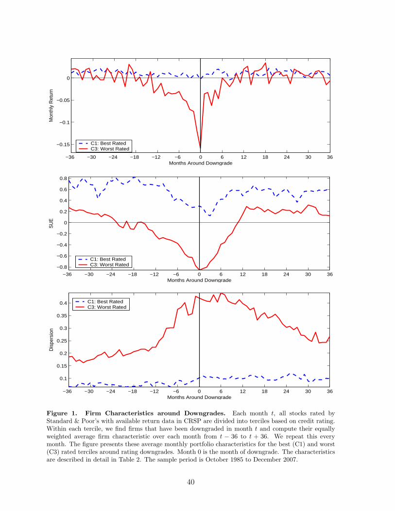
−36 −30 −24 −18 −12 −6 0 6 12 18 24 30 36

−0.15

−0.1

−0.05

0

Months Around Downgrade

Mon

thly

Ret

urn

C1: Best RatedC3: Worst Rated

−36 −30 −24 −18 −12 −6 0 6 12 18 24 30 36

−0.8

−0.6

−0.4

−0.2

0

0.2

0.4

0.6

0.8

Months Around Downgrade

SU

E

C1: Best RatedC3: Worst Rated

−36 −30 −24 −18 −12 −6 0 6 12 18 24 30 36

0.1

0.15

0.2

0.25

0.3

0.35

0.4

Months Around Downgrade

Dis

pers

ion

C1: Best RatedC3: Worst Rated

Figure 1. Firm Characteristics around Downgrades. Each month t, all stocks rated byStandard & Poor’s with available return data in CRSP are divided into terciles based on credit rating.Within each tercile, we find firms that have been downgraded in month t and compute their equallyweighted average firm characteristic over each month from t − 36 to t + 36. We repeat this everymonth. The figure presents these average monthly portfolio characteristics for the best (C1) and worst(C3) rated terciles around rating downgrades. Month 0 is the month of downgrade. The characteristicsare described in detail in Table 2. The sample period is October 1985 to December 2007.

40

−36 −30 −24 −18 −12 −6 0 6 12 18 24 30 36

0.02

0.04

0.06

0.08

0.1

0.12

Months Around Downgrade

Idio

sync

ratic

Vol

atili

ty

C1: Best RatedC3: Worst Rated

−36 −30 −24 −18 −12 −6 0 6 12 18 24 30 36

−0.035

−0.03

−0.025

−0.02

−0.015

−0.01

−0.005

0

0.005

Months Around Downgrade

Acc

rual

s

C1: Best RatedC3: Worst Rated

−36 −30 −24 −18 −12 −6 0 6 12 18 24 30 36

0.8

1

1.2

1.4

1.6

1.8

2

2.2

Months Around Downgrade

Boo

k−to

−Mar

ket R

atio

C1: Best RatedC3: Worst Rated

Figure 1(continued). Firm Characteristics around Downgrades.

41